Module 4 Boundary value problems in linear elasticityweb.mit.edu/16.20/homepage/4_ElasticityBVP/ElasticityBVP_files/... · Module 4 Boundary value problems in linear elasticity Learning

Module 4

Boundary value problems in linearelasticity

Learning Objectives

• formulate the general boundary value problem of linear elasticity in three dimensions

• understand the stress and displacement formulations as alternative solution approachesto reduce the dimensionality of the general elasticity problem

• solve uniform states of strain and stress in three dimensions

• specialize the general problem to planar states of strain and stress

• understand the stress function formulation as a means to reduce the general problemto a single differential equation.

• solve aerospace-relevant problems in plane strain and plane stress in cartesian andcylindrical coordinates.

4.1 Summary of field equations

Readings: BC 3 Intro, Sadd 5.1

• Equations of equilibrium ( 3 equations, 6 unknowns ):

σji,j + fi = 0 (4.1)

• Compatibility ( 6 equations, 9 unknowns):

εij =1

2

(∂ui∂xj

+∂uj∂xi

)(4.2)

77

http://library.books24x7.com.libproxy.mit.edu/assetviewer.aspx?bookid=37241&chunkid=366405095&rowid=204&noteMenuToggle=0&leftMenuState=1

78 MODULE 4. BOUNDARY VALUE PROBLEMS IN LINEAR ELASTICITY

e1

e2

e3

B

b

f

b∂Bu

u

t

∂Bt

b

u

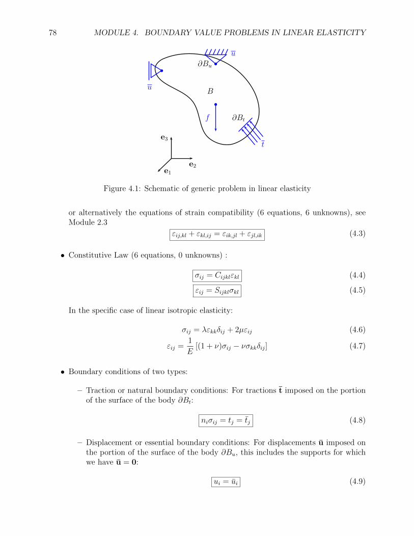
Figure 4.1: Schematic of generic problem in linear elasticity

or alternatively the equations of strain compatibility (6 equations, 6 unknowns), seeModule 2.3

εij,kl + εkl,ij = εik,jl + εjl,ik (4.3)

• Constitutive Law (6 equations, 0 unknowns) :

σij = Cijklεkl (4.4)

εij = Sijklσkl (4.5)

In the specific case of linear isotropic elasticity:

σij = λεkkδij + 2µεij (4.6)

εij =1

E[(1 + ν)σij − νσkkδij] (4.7)

• Boundary conditions of two types:

– Traction or natural boundary conditions: For tractions t imposed on the portionof the surface of the body ∂Bt:

niσij = tj = tj (4.8)

– Displacement or essential boundary conditions: For displacements u imposed onthe portion of the surface of the body ∂Bu, this includes the supports for whichwe have u = 0:

ui = ui (4.9)

4.2. SOLUTION PROCEDURES 79

We observe that the general elasticity problem contains 15 unknown fields: displacements(3), strains (6) and stresses (6); and 15 governing equations: equilibrium (3), pointwisecompatibility (6), and constitutive (6), in addition to suitable displacement and tractionboundary conditions. One can prove existence and uniqueness of the solution ( the fields:ui(xj), εij(xk), σij(xk)) in B assuming the convexity of the strain energy function or thepositive definiteness of the stiffness tensor.

It can be shown that the system of equations has a solution (existence) which is unique(uniqueness) providing that the bulk and shear moduli are positive:

K =E

3(1− 2ν)> 0, G =

E

2(1 + ν)> 0

which poses the following restrictions on the Poisson ratio:

−1 < ν < 0.5

4.2 Solution Procedures

The general problem of 3D elasticity is very difficult to solve analytically in general. Thefirst step in trying to tackle the solution of the general elasticity problem is to reduce thesystem to fewer equations and unknowns by a process of elimination. Depending on theprimary unknown of the resulting equations we have the:

4.2.1 Displacement formulation

Readings: BC 3.1.1, Sadd 5.4

In this case, we try to eliminate the strains and stresses from the general problem andseek a reduced set of equations involving only displacements as the primary unknowns. Thisis useful when the displacements are specified everywhere on the boundary. The formula-tion can be readily derived by first replacing the constitutive law, Equations (4.4) in theequilibrium equations, Equations (4.1):(

Cijklεkl),j

+ fi = 0

and then replacing the strains in terms of the displacements using the stress-strain relations,Equations (4.2): (

Cijkluk,l),j

+ fi = 0 (4.10)

These are the so-called Navier equations. Once the displacement field is found, the strainsfollow from equation (4.2), and the stresses from equation (4.4).

Concept Question 4.2.1. Navier’s equations.



Specialize the general Navier equations to the case of isotropic elasticity So-lution: The strategy is to replace the strain-displacement relations in the constitutive lawfor isotropic elasticity

σij = λεkkδij + 2µεij

= λuk,kδij + µ(ui,j + uj,i),

and then insert this in the equilibrium equations:

0 = σij,j + fi = λuk,kjδij + µ(ui,jj + uj,ij) + fi

= λuk,ki + µ(ui,jj + uj,ij) + fi.

This can be slightly simplified to finally obtain:

(λ+ µ)uj,ji + µui,jj + fi = 0

It can be observed that this is the component form of the vector equation:

(λ+ µ)∇ · (∇u) + µ∇2u + f = 0.

Concept Question 4.2.2. Harmonic volumetric deformation.Show that in the case that the body forces are uniform or vanish the volumetric defor-

mation e = εkk = uk,k is harmonic, i.e. its Laplacian vanishes identically:

∇2e = e,ii = 0.

(Hint: apply the divergence operator ()i,i to Navier’s equations) Solution:[(λ+ µ)uj,ji + µui,jj + fi

],i

= 0[(λ+ µ)e,i + µui,jj + fi

],i

= 0

(λ+ µ)e,ii + µui,jji + fi,i = 0

(λ+ µ)e,ii + µe,jj + fi,i = 0

(λ+ 2µ)e,ii + fi,i = 0.

If fi is zero or constant, fi,i = 0 and we obtain the sought result

e,ii =∂2e

∂xi2= 0


Concept Question 4.2.3. A solution to Navier’s equations.Consider a problem with body forces given by

f =

f1

f2

f3

=

−6Gx2x3

2Gx1x3

10Gx1x2

,where G = E

2(1+ν)and ν = 1/4.

Assume displacements given by

u =

u1

u2

u3

=

C1x21x2x3

C2x1x22x3

C3x1x2x23

.Determine the constants, C1, C2, and C3 allowing the displacement field u to be solution

of the Navier equations. Solution: By applying the Navier’s equations

E

2(1 + ν)(1− 2ν)uj,ji +

E

2(1 + ν)ui,jj + fi = 0

E

2(1 + ν)(1− 2ν)e,i +

E

2(1 + ν)ui,jj + fi = 0,

where e = εkk = uk,k.For this specific problem, the Navier equations can be simplified to

2Guj,ji +Gui,jj + fi = 0

2Ge,i +Gui,jj + fi = 0.

From the displacement field we can calculate

u1 = C1x21x2x3, u1,1 = ε11 = 2C1x1x2x3, u1,11 = 2C1x2x3, u1,22 = u1,33 = 0,



e = ε11 + ε22 + ε33 = 2(C1 + C2 + C3)x1x2x3.

Introducing the above expressions into the Navier’s equations, we obtain

(6C1 + 4C2 + 4C3 − 6)Gx2x3 = 0

(4C1 + 6C2 + 4C3 + 2)Gx1x3 = 0

(4C1 + 4C2 + 6C3 + 10)Gx1x2 = 0,

which allows us to write the following system of equations6 4 44 6 44 4 6

C1

C2

C3

=

6−2−10

.


The solution of this algebraic system is (C1, C2, C3) = 17(27,−1,−29), which leads to the

following displacement field

u =

u1

u2

u3

=1

7

27x21x2x3

−x1x22x3

−29x1x2x23

.

Practical solutions of Navier’s equations can be obtained for fairly complex elasticityproblems via the introduction of displacement potential functions to further simplify theequations.

4.2.2 Stress formulation

Readings: Sadd 5.3

In this case we attempt to eliminate the displacements and strains and obtain equationswhere the stress components are the only unknowns. This is useful when the tractionsare specified on the boundary. To eliminate the displacements, instead of using the strain-displacement conditions to enforce compatibility, it is more convenient to use the SaintVenant compatibility equations (4.3) The derivation is based on replacing the constitutivelaw, Equations (4.4) into these equations, and then use the equilibrium equations (4.1), i.e.the first step involves doing:

(Sijmnσmn︸︷︷︸εij

),kl + (Sklmnσmn︸︷︷︸εkl

),ij = (Sikmnσmn︸︷︷︸εik

),jl + (Silmnσmn︸︷︷︸εjl

),ik (4.11)

Concept Question 4.2.4. Beltrami-Michell’s equations.Derive the Beltrami-Michell equations corresponding to isotropic elasticity (Hint: as

a first step, use the compliance form of the isotropic elasticity constitutive relations andreplace them into the Saint-Venant strain compatibility equations, if you take it this far, Iwill explain some additional simplifications) Solution: The general expression for thestress compatibility conditions is given by

εij,kl + εkl,ij = εik,jl + εjl,ik,

but it is possible to find the six meaningful relationships by setting k = l, i.e.

εij,kk + εkk,ij = εik,jk + εjk,ik.

Introducing the compliance expression for isotropic materials

εmn =1

E[(1 + ν)σmn − νσppδmn]



into the compatibility expressions, we obtain that

1

E[(1 + ν)σij,kk − νσpp,kkδij] +

1

E[(1 + ν)σkk,ij − νσpp,ijδkk] =

1

E[(1 + ν)σik,jk − νσpp,jkδik] +

1

E[(1 + ν)σjk,ik − νσpp,ikδjk] ,

and after a little algebra we can write

σij,kk + σkk,ij − σik,jk − σjk,ik = − ν

1 + ν[σpp,jkδik + σpp,ikδjk − σpp,kkδij − σpp,ijδkk]

σij,kk + σkk,ij − σik,jk − σjk,ik = − ν

1 + ν[σpp,ij + σpp,ij − σpp,kkδij − 3σpp,ij]

σij,kk + σkk,ij − σik,jk − σjk,ik =ν

1 + νσkk,ij +

ν

1 + νσpp,kkδij.

Using the equilibrium equations σij,j + fi = 0, the above expresion can be simplified to

σij,kk +1

1 + νσkk,ij =

ν

1 + νσpp,kkδij − fi,j − fj,i. (4.12)

For the case i = j, the previous equation reduces to

σii,kk +1

1 + νσkk,ii =

3ν

1 + νσpp,kk − 2fi,i

σii,kk +1

1 + νσii,kk =

3ν

1 + νσii,kk − 2fi,i

σii,kk = σpp,kk = − 1 + ν

1− νfi,i = − 1 + ν

1− νfk,k,

which allows us to write the Equation 4.12 as

σij,kk +1

1 + νσkk,ij = − ν

1− νfk,kδij − fi,j − fj,i

Concept Question 4.2.5. Beltrami-Michell’s equations expanded.Consider the case of constant body forces. Expand the general Beltrami-Michell equations

written in index form into the six independent scalar equations Solution: TheBeltrami-Michell’s equations in index notation are written as

σij,kk +1

1 + νσkk,ij = − ν

1− νfk,kδij − fi,j − fj,i,

and for constant body forces they reduce to

(1 + ν)σij,kk + σkk,ij = 0.


(1 + ν)∇2σ11 +∂2

∂x21

(σ11 + σ22 + σ33) = (1 + ν)∇2σ11 +∂2I1

∂x21

= 0

(1 + ν)∇2σ22 +∂2

∂x22

(σ11 + σ22 + σ33) = (1 + ν)∇2σ22 +∂2I1

∂x22

= 0

(1 + ν)∇2σ33 +∂2

∂x23

(σ11 + σ22 + σ33) = (1 + ν)∇2σ33 +∂2I1

∂x23

= 0

(1 + ν)∇2σ12 +∂2

∂x1∂x2

(σ11 + σ22 + σ33) = (1 + ν)∇2σ12 +∂2I1

∂x1∂x2

= 0

(1 + ν)∇2σ13 +∂2

∂x1∂x3

(σ11 + σ22 + σ33) = (1 + ν)∇2σ13 +∂2I1

∂x1∂x3

= 0

(1 + ν)∇2σ23 +∂2

∂x2∂x3

(σ11 + σ22 + σ33) = (1 + ν)∇2σ23 +∂2I1

∂x2∂x3

= 0,

where ∇2 = ∂2

∂x21+ ∂2

∂x22+ ∂2

∂x23and I1 = σ11 +σ22 +σ33 is the first invariant of the stress tensor.

Of the six non-vanishing equations obtained, only three represent independent equations(just as with Saint-Venant strain compatibility equations). Combining these with the threeequations of equilibrium provides the necessary six equations to solve for the six unknownstress components.

Once the stresses have been found, one can use the constitutive law to determine thestrains, and the strain-displacement relations to compute the displacements.

As we will see in 2D applications, the Beltrami-Michell equations are still very difficultto solve. We will introduce the concept of stress functions to further reduce the equations.

4.3 Principle of superposition

Readings: Sadd 5.5

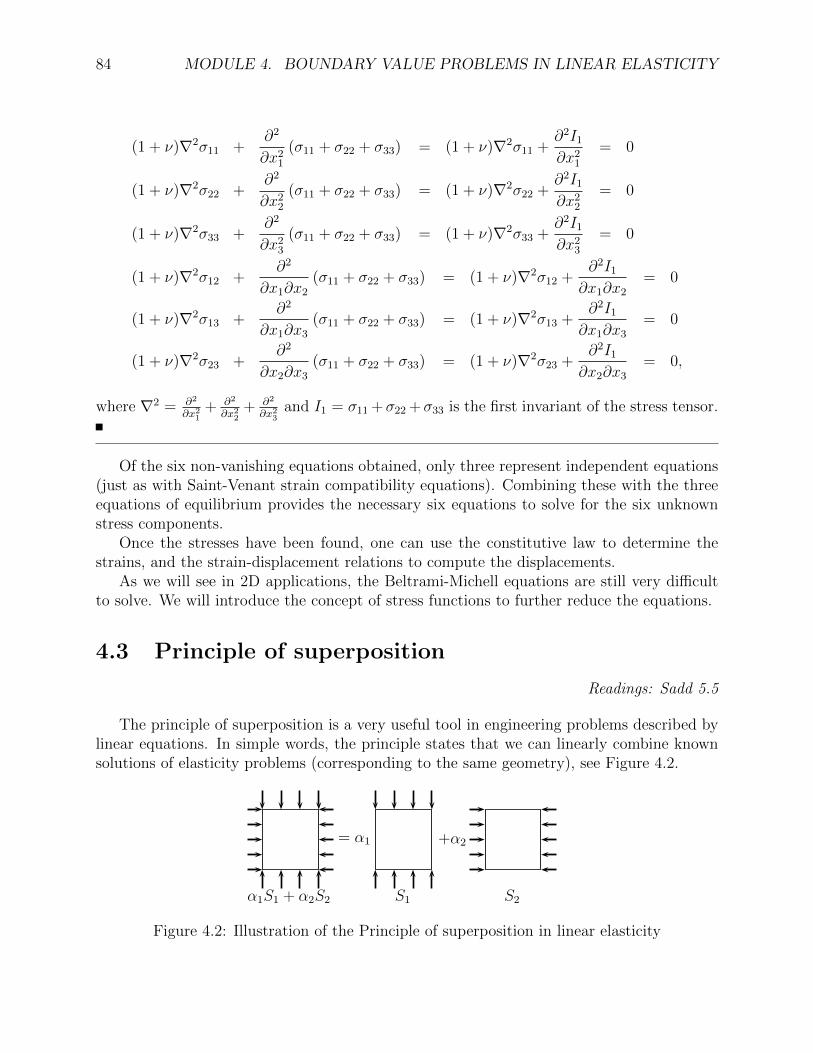
The principle of superposition is a very useful tool in engineering problems described bylinear equations. In simple words, the principle states that we can linearly combine knownsolutions of elasticity problems (corresponding to the same geometry), see Figure 4.2.

α1S1 + α2S2

= α1 +α2

S1 S2

Figure 4.2: Illustration of the Principle of superposition in linear elasticity


4.4. SAINT VENANT’S PRINCIPLE 85

4.4 Saint Venant’s Principle

Readings: Sadd 5.6

Saint Venant’s Principle states the following:

The elastic fields (stres, strain, displacement) resulting from two different but staticallyequivalent loading conditions are approximately the same everywhere except in the vicinityof the point of application of the load.

Figure 4.3 provides an illustration of the idea. This principle is extremely useful in struc-

PP

2

P

2

P

3

P

3

P

3

Figure 4.3: Illustration of Saint Venant’s Principle

tural mechanics, as it allows the possibility to idealize and simplify loading conditions whenthe details are complex or missing, and develop analytically tractable models to analyze thestructure of interest. One can after perform a detailed analysis of the elastic field surround-ing the point of application of the load (e.g. think of a riveted joint in an aluminum framestructure).

Although the principle was stated in a rather intuitive way by Saint Venant, it has beendemonstrated analytically in a convincing manner.

4.5 Solution methods

Readings: Sadd 5.7




4.5.1 Direct Integration

The general idea is to try to integrate the system of partial differential equations analytically.Problems involving simple geometries and loading conditions which result in stress fields withuniform or linear spatial distributions can be attacked by simple calculus methods.

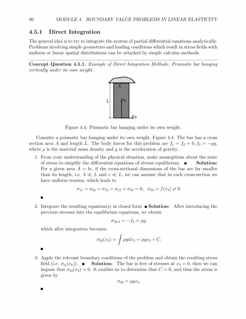
Concept Question 4.5.1. Example of Direct Integration Methods: Prismatic bar hangingvertically under its own weight.

L

e2

e3

b

A

Figure 4.4: Prismatic bar hanging under its own weight.

Consider a prismatic bar hanging under its own weight, Figure 4.4. The bar has a crosssection area A and length L. The body forces for this problem are f1 = f2 = 0, f3 = −ρg,where ρ is the material mass density and g is the acceleration of gravity.

1. From your understanding of the physical situation, make assumptions about the stateof stress to simplify the differential equations of stresss equilibrium. Solution:For a given area A = bc, if the cross-sectional dimensions of the bar are far smallerthan its length, i.e. b L and c L, we can assume that in each cross-section wehave uniform tension, which leads to

σ11 = σ22 = σ12 = σ13 = σ23 = 0, σ33 = f(x3) 6= 0.

2. Integrate the resulting equation(s) in closed form Solution: After introducing theprevious stresses into the equilibrium equations, we obtain

σ33,3 = −f3 = ρg,

which after integration becomes

σ33(x3) =

∫ρgdx3 = ρgx3 + C.

3. Apply the relevant boundary conditions of the problem and obtain the resulting stressfield (i.e. σij(xk)). Solution: The bar is free of stresses at x3 = 0, then we canimpose that σ33(x3) = 0. It enables us to determine that C = 0, and thus the stress isgiven by

σ33 = ρgx3.

4.5. SOLUTION METHODS 87

4. Use the constitutive equations to compute the strain components. Solution:From Hooke’s law, we directly obtain:

ε11 = u1,1 = − νρgx3

E, (4.13)

ε22 = u2,2 = − νρgx3

E, (4.14)

ε33 = u3,3 =ρgx3

E, (4.15)

ε23 =1

2(u2,3 + u3,2) = 0, (4.16)

ε13 =1

2(u1,3 + u3,1) = 0, (4.17)

ε12 =1

2(u1,2 + u2,1) = 0. (4.18)

5. Integrate the strain-displacement relations and apply boundary conditions to obtainthe displacement field. Solution:

After the integration of Eq. 4.15, we obtain

u3 =ρg

2Ex2

3 + g1(x1, x2), (4.19)

where g1(x1, x2) is an arbitrary function arising from the integration.

From Eqs. 4.17 and 4.16 we know that u1,3 = −u3,1 and u2,3 = −u3,2, which incombination with eq. 4.19 leads to

u1,3 = −g1,1(x1, x2), u2,3 = −g1,2(x1, x2).

After integration we obtain

u1 = −g1,1(x1, x2)x3 + g2(x1, x2), (4.20)

u2 = −g1,2(x1, x2)x3 + g3(x1, x2), (4.21)

where g2(x1, x2) and g3(x1, x2) are arbitrary functions coming from the integration.

By replacing Eqs. 4.20 and 4.21 into Eqs. 4.13 and 4.14, we find that

−g1,11(x1, x2)x3 + g2,1(x1, x2) = −νρgx3

E

−g1,22(x1, x2)x3 + g3,2(x1, x2) = −νρgx3

E,

which can be rearranged as(g1,11(x1, x2)− νρg

E

)x3 = g2,1(x1, x2)(

g1,22(x1, x2)− νρg

E

)x3 = g3,2(x1, x2).


As these equations must hold for any value of x3, the expressions in parentheses andthe right hand side must vanish (note that they only depend on x1 and x2), whichleads to

g1,11(x1, x2) =νρg

E, (4.22)

g1,22(x1, x2) =νρg

E, (4.23)

g2,1(x1, x2) = 0, (4.24)

g3,2(x1, x2) = 0.. (4.25)

After integration we obtain

g1(x1, x2) =νρg

2Ex2

1 +m1(x2)x1 + A1, (4.26)

g1(x1, x2) =νρg

2Ex2

2 +m2(x1)x2 + A2, (4.27)

g2(x1, x2) = m3(x2) + A3, (4.28)

g3(x1, x2) = m4(x1) + A4, (4.29)

where m1(x2), m2(x1), m3(x2), m4(x1) are arbitrary functions, while A1, A2, A3 andA4 are arbitrary constants.

From Eqs. 4.18, 4.20 and 4.21 we also know that

u1,2 + u2,1 = −2g1,12(x1, x2)x3 + g2,2(x1, x2) + g3,1(x1, x2) = 0,

and considering that this expression must hold for any value of x3, the following equa-tions must satisfy

g1,12(x1, x2) = 0, (4.30)

g2,2(x1, x2) + g3,1(x1, x2) = 0. (4.31)

By replacing Eqs. 4.28 and 4.29 into Eq. 4.31, we can write

m3,2(x2) +m4,1(x1) = 0,

whose only possible solution is m3(x2) = A5x2, and m4(x1) = −A5x1. This result leadsto

g2(x1, x2) = A5x2 + A3, (4.32)

g3(x1, x2) = −A5x1 + A4. (4.33)

From Eqs. 4.26, 4.27 and 4.30, we can derive

g1,12(x1, x2) = m1,2(x2) = m2,1(x1) = 0

4.5. SOLUTION METHODS 89

and hence m1(x2) = A6 and m2(x1) = A7, where A6 and A7 are arbitrary constants.With the help of superposition, we can write the following expression for g1(x1, x2)

g1(x1, x2) =νρg

2E

(x2

1 + x22

)+ A6x1 + A7x2 + A8. (4.34)

The Eqs 4.19, 4.20, 4.21, 4.32, 4.33 and 4.34 allow us to write the general solution forthe displacement field

u1 = −νρgEx1x3 + A5x2 − A6x3 + A3,

u2 = −νρgEx2x3 − A5x1 − A7x3 + A4,

u3 =ρg

2Ex2

3 +νρg

2E

(x2

1 + x22

)+ A6x1 + A7x2 + A8.

The 6 constants are determined by imposing 3 displacements (u1(0, 0, L) = u2(0, 0, L) =u3(0, 0, L) = 0) and 3 rotations (ω1(0, 0, L) = ω2(0, 0, L) = ω3(0, 0, L) = 0)

u1 = −νρgEx1x3,

u2 = −νρgEx2x3,

u3 =ρg

2E

[x2

3 − L2 + ν(x2

1 + x22

)].

6. Compute the axial displacement at the tip of the bar and compare with the solutionobtained with the one-dimensional analysis. Solution:

The axial displacement at the tip (x3 = 0) of the prismatic bar is

u3 = − ρg2E

[L2 − ν(x2

1 + x22)],

which reduces to utip3 = − ρg2EL2 at the centerline (x1 = x2 = 0).

For the one-dimensional analysis we can write the weight of the bar as P = −ρAgx. Thestress is uniform in each cross section, and then can be calculated as σ = P/A = −ρgx.The stress-strain relation satisfies σ = Eε, which allows us to compute the displacementas

utip =

∫ L

0

εdx =

∫ L

0

σ

Edx = −ρg

E

∫ L

0

xdx = −ρgL2

2E.

The displacements utip and utip3 are equal. It means that the one-dimensional analysisshows the same behavior that the centerline of the three-dimensional approach. Whenthe finite dimension of the cross section is considered, the vertical displacement awayfrom the centerline is reduced by a factor proportional to Poisson’s ratio and the squareof the distance from the centerline.


7. Compute the axial displacement at the tip of the bar and compare with the solutionfor a weightless bar subject to a point load P = −ρgAL. Solution: The axialdisplacement at the tip (x3 = 0) and centerline (x1 = x2 = 0) of the prismatic bar is

utip3 = − ρg2E

L2.

When the bar is subject to a point load P = −ρgAL, the stress satisfies σ = P/A =−ρgL. Since the stress-strain relation is given by σ = Eε, we can calculate the dis-placement as

utip =

∫ L

0

εdx =

∫ L

0

σ

Edx = −ρgL

E

∫ L

0

dx = −ρgL2

E.

We observe that utip is the double of utip3 .

More complex situations require advanced analytical techniques and mathematical meth-ods including: power and Fourier series, integral transforms (Fourier, Laplace, Hankel),complex variables, etc.

4.5.2 Inverse Method

In this method, one selects a particular displacement or stress field distribution which satisfythe field equations a priori and then investigates what physical situation they correspond toin terms of geometry, boundary conditions and body forces. It is usually difficult to use thisapproach to obtain solutions to problems of specific practical interest.

4.5.3 Semi-inverse Method

This is similar in concept to the inverse method, but the idea is to adopt a “general form”of the variation of the assumed field, sometimes informed by some assumption about thephysical response of the system, with unknown constants or functions of reduced dimension-ality. After replacing the assumed functional form into the field equations the system canbe reduced in number of unknowns and dimensionality. The reduced system can typicallybe integrated explicitly by the direct or analytical methods.

This is the approach that leads to the very important theories of torsion of prismaticbars, and theory of structural elements (trusses, beams, plates and shells). We will discussthese theories in detail later in this class.

4.6 Two-dimensional Problems in Elasticity

Readings: Sadd, Chapter 7

In many cases of practical interest, the three-dimensional problem can be reduced to twodimensions. We will consider two of the basic 2-D elasticity problem types:

4.6. TWO-DIMENSIONAL PROBLEMS IN ELASTICITY 91

4.6.1 Plane Stress

Readings: Sadd 7.2

As the name indicates, the only stress components are in a plane, i.e. there are noout-of-plane stress components.

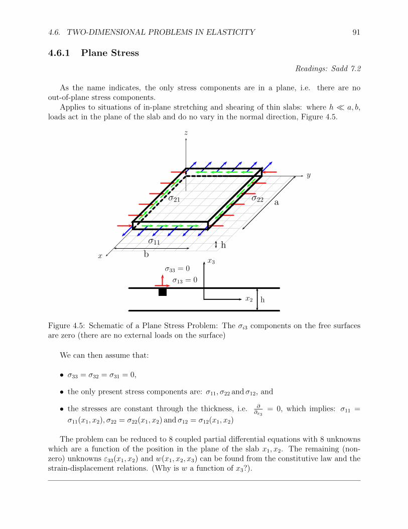
Applies to situations of in-plane stretching and shearing of thin slabs: where h a, b,loads act in the plane of the slab and do no vary in the normal direction, Figure 4.5.

x

y

z

σ11

σ22σ21 a

bh

x3

x2

σ33 = 0

σ13 = 0

h

Figure 4.5: Schematic of a Plane Stress Problem: The σi3 components on the free surfacesare zero (there are no external loads on the surface)

We can then assume that:

• σ33 = σ32 = σ31 = 0,

• the only present stress components are: σ11, σ22 andσ12, and

• the stresses are constant through the thickness, i.e. ∂∂x3

= 0, which implies: σ11 =

σ11(x1, x2), σ22 = σ22(x1, x2) andσ12 = σ12(x1, x2)

The problem can be reduced to 8 coupled partial differential equations with 8 unknownswhich are a function of the position in the plane of the slab x1, x2. The remaining (non-zero) unknowns ε33(x1, x2) and w(x1, x2, x3) can be found from the constitutive law and thestrain-displacement relations. (Why is w a function of x3?).

http://library.books24x7.com.libproxy.mit.edu/assetviewer.aspx?bookid=37241&chunkid=405897568&noteMenuToggle=0&leftMenuState=1


Concept Question 4.6.1. Governing equations for plane stress.Obtain the full set of governing equations for plane stress by specializing the general 3-D

elasticity problem based on the plane-stress assumptions. Do the same for the Navier andBeltrami-Michell equations.

Solution:Assumption:

σi3 = 0 ⇒ σ13 = σ23 = σ33 = 0.

Equilibrium equations reduce to:

∂σ11

∂x1

+∂σ12

∂x2

+ f1(x1, x2) = 0

∂σ12

∂x1

+∂σ22

∂x2

+ f2(x1, x2) = 0.

Constitutive equations reduce to:

ε11 =1

E

(σ11 − νσ22

)ε22 =

1

E

(σ22 − νσ11

)ε33 = − ν

E

(σ11 + σ22

)= − ν

1− ν(ε11 + ε22)

ε12 =1

2Gσ12 =

(1 + ν)

Eσ12

ε23 = 0

ε13 = 0.

Strain-displacements relations reduce to:

ε11 =∂u1

∂x1

, ε22 =∂u2

∂x2

, ε33 =∂u3

∂x3

2ε12 =∂u1

∂x2

+∂u2

∂x1

.

Navier equations (start from the equilibrium equation σij,j + fi = 0 and introduce thestrain-stress relationship):

E

2(1 + ν)∇2u1 +

E

2(1− ν)

∂

∂x1

(∂u1

∂x1

+∂u2

∂x2

)+ f1 = 0

E

2(1 + ν)∇2u2 +

E

2(1− ν)

∂

∂x2

(∂u1

∂x1

+∂u2

∂x2

)+ f2 = 0.

Beltrami-Michell equations (start from the Saint-Venant compatibility condition for 2Dproblems ε11,22 + ε22,11 = 2ε12,12 and introduce the strain-stress relationship):

∇2(σ11 + σ22) = −(1 + ν)

(∂f1

∂x1

+∂f2

∂x2

).

4.6. TWO-DIMENSIONAL PROBLEMS IN ELASTICITY 93

4.6.2 Plane Strain

Readings: Sadd 7.1

Consider elasticity problems such as the one in Figure 4.6. In this case, L is muchlarger than the transverse dimensions of the structure, the loads applied are parallel to thex1x2 plane and do not change along x3. It is clear that the solution cannot vary along x3,i.e. the same stresses and strains must be experienced by any slice along the x3 axis. Wetherefore need to only analyze the 2-D solution in a generic slice, as shown in the figure. Bysymmetry with respect to the x3 axis, there cannot be any displacements or body forces inthat direction.

.We can then assume that:

u3 = 0,∂(.)

∂x3

= 0 (4.35)

From this we can conclude that: ε33 = ε13 = ε23 = 0, and the only strain componentsare those “in” the plane: ε11, ε22, ε12, which are only a function of x1 and x2.

Concept Question 4.6.2. Governing equations for plane strain.Obtain the full set of governing equations for plane strain by specializing the general 3-D

elasticity problem based on the plane-strain assumptions. Do the same for the Navier andBeltrami-Michell equations.

Solution:Assumption:

εi3 = 0 ⇒ ε13 = ε23 = ε33 = 0.

Equilibrium equations reduce to:

∂σ11

∂x1

+∂σ12

∂x2

+ f1(x1, x2) = 0

∂σ12

∂x1

+∂σ22

∂x2

+ f2(x1, x2) = 0.

Constitutive equations reduce to:

ε11 =1 + ν

E[(1− ν)σ11 − νσ22]

ε22 =1 + ν

E[(1− ν)σ22 − νσ11]

ε33 = 0 ⇒ σ33 = ν (σ11 + σ22) =νE

(1 + ν)(1− 2ν)(ε11 + ε22)

ε12 =1

2Gσ12 =

(1 + ν)

Eσ12

ε23 = 0

ε23 = 0.



x3 x1

x2

..

x3 x1

x2

Figure 4.6: Schematic of a typical situation where plane-strain conditions apply and there isonly need to analyze the solution for a generic slice with constrained displacements normalto it

4.7. AIRY STRESS FUNCTION 95

Strain-displacements relations reduce to:

ε11 =∂u1

∂x1

, ε22 =∂u2

∂x2

, ε33 = 0

2ε12 =∂u1

∂x2

+∂u2

∂x1

.

Navier equations (start from the equilibrium equation σij,j + fi = 0 and introduce thestrain-stress relationship):

E

2(1 + ν)∇2u1 +

E

2(1 + ν)(1− 2ν)

∂

∂x1

(∂u1

∂x1

+∂u2

∂x2

)+ f1 = 0

E

2(1 + ν)∇2u2 +

E

2(1 + ν)(1− 2ν)

∂

∂x2

(∂u1

∂x1

+∂u2

∂x2

)+ f2 = 0.

Beltrami-Michell equations (start from the Saint-Venant compatibility condition for 2Dproblems ε11,22 + ε22,11 = 2ε12,12 and introduce the strain-stress relationship):

∇2(σ11 + σ22) = − 1

1− ν

(∂f1

∂x1

+∂f2

∂x2

).

4.7 Airy stress function

Readings: Sadd 7.5

A very useful technique in solving plane stress and plane strain problems is to introducea scalar stress function φ(x1, x2) such that all the relevant unknown stress components arefully determined from this single scalar function. The specific dependence to be consideredis:

σ11 =∂2φ

∂x22

(4.36)

σ22 =∂2φ

∂x12

(4.37)

σ12 = − ∂2φ

∂x1∂x2

(4.38)

This choice, although apparently arbitrary, results in two significant simplifications in ourgoverning equations:

Concept Question 4.7.1. Airy stress function and equilibrium conditions.Show that the particular choice of stress function given automatically satisfies the stress

equilibrium equations in 2D for the case of no body forces. Solution: For a system freeof body forces, the equilibrium equations reduce to

σij,j = 0.



By introducingσ11 = φ,22, σ22 = φ,11, σ12 = −φ,12,

it is straightforward to verify that

σ11,1 + σ12,2 = φ,221 − φ,122 = 0

σ21,1 + σ22,2 = −φ,121 + φ,112 = 0.

Concept Question 4.7.2. Two-dimensional biharmonic PDE.Obtain a scalar partial differential equation for 2D elasticity problems with no body

forces whose only unknown is the stress function (Hint: replace the stresses in the Beltrami-Michell equations for 2D (plane strain or stress) with no body forces in terms of the Airystress function. The final result should be:

φ,1111 + 2φ,1122 + φ,2222 = 0 (4.39)

This can also be written using the ∇ operator (see Appendix ??) as:

∇4φ =

∂2

∂x12

+∂2

∂x22︸︷︷︸

∇2

2

φ (4.40)

Solution: Starting from the compatibility conditions for 2D problems

ε11,22 + ε22,11 = 2ε12,12,

and introducing the compliance form of the plane stress approach

ε11 =1

E(σ11 − νσ22)

ε22 =1

E(σ22 − νσ11)

ε12 =1 + ν

Eσ12,

we arrive toσ11,22 − νσ22,22 + σ22,11 − νσ11,11 = 2(1 + ν)σ12,12. (4.41)

Considering thatσ11 = φ,22, σ22 = φ,11, σ12 = −φ,12,

we can rewrite the Equation 4.41 as

φ,2222 − νφ,1122 + φ,1111 − νφ,2211 = −2(1 + ν)φ,1212,


which reduces toφ,1111 + 2φ,1212 + φ,2222 = 0.

This last PDE is so-called biharmonic equation, and is also expressed as

∇4φ = ∇2∇2φ = 0.

NB: we arrive to the same equation using the compliance form of the plane strain ap-proach.

4.7.1 Problems in Cartesian Coordinates

Readings: Sadd 8.1

A number of useful solutions to problems in rectangular domains can be obtained byadopting stress functions with polynomial distribution.

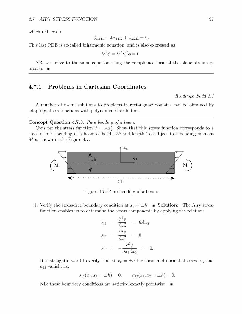
Concept Question 4.7.3. Pure bending of a beam.Consider the stress function φ = Ax3

2. Show that this stress function corresponds to astate of pure bending of a beam of height 2h and length 2L subject to a bending momentM as shown in the Figure 4.7.

e1

e2

MM2h

2L

Figure 4.7: Pure bending of a beam.

1. Verify the stress-free boundary condition at x2 = ±h. Solution: The Airy stressfunction enables us to determine the stress components by applying the relations

σ11 =∂2φ

∂x22

= 6Ax2

σ22 =∂2φ

∂x21

= 0

σ12 = − ∂2φ

∂x1∂x2

= 0.

It is straightforward to verify that at x2 = ±h the shear and normal stresses σ12 andσ22 vanish, i.e.

σ12(x1, x2 = ±h) = 0, σ22(x1, x2 = ±h) = 0.

NB: these boundary conditions are satisfied exactly pointwise.

http://library.books24x7.com.libproxy.mit.edu/assetviewer.aspx?bookid=37241&chunkid=364412640


2. Establish a relation between M and the stress distribution at the beam ends in integralform to fully define the stress field in terms of problem parameters. Solution:The following integral conditions must also be satisfied∫ h

−hσ11(x1 ± L, x2)dx2 = 0,

∫ h

−hσ11(x1 ± L, x2)x2dx2 = −M.

This last equation allows us to calculate the constant A in function of the parametersM and h: ∫ h

−hσ11(x1 ± L, x2)x2dx2 = −M = 4Ah3 ⇒ A = − M

4h3,

and then the stress field becomes

σ12 = σ22 = 0, σ11 = −3M

2h3x2.

3. Integrate the strain-displacement relations to obtain the displacement field. What doesthe undetermined function represent? Solution:By applying the strain-displacement conditions and the strain-stress relationships forplain stress, we obtain that

ε11 = − 3M

2Eh3x2 =

∂u1

∂x1

⇒ u1(x1, x2) = − 3M

2Eh3x2x1 + f(x2)

ε22 = ν3M

2Eh3x2 =

∂u2

∂x2

⇒ u2(x1, x2) = ν3M

4Eh3x2

2 + g(x1)

ε12 = 0 =1

2

(∂u1

∂x2

+∂u2

∂x1

)⇒ − 3M

2Eh3x1 +

dg(x1)

dx1

+df(x2)

dx2

= 0,

where g(x1) and f(x2) are arbitrary functions of integration.

The last equation can be separated into two independent relations in x1 and x2

− 3M

2Eh3x1 +

dg(x1)

dx1

= C1,df(x2)

dx2

= −C1,

which leads to

f(x2) = −C1x2 + C2,

and

g(x1) =3M

4Eh3x2

1 + C1x+ C3.

By replacing these functions in the expressions for displacement, we obtain

u1(x1, x2) = − 3M

2Eh3x2x1−C1x2 +C2, u2(x1, x2) = ν

3M

4Eh3x2

2 +3M

4Eh3x2

1 +C1x+C3.


The integration constants C1, C2 and C3 can be determined by imposing the conditionsu1(0, x2) = 0 and u2(±L, 0) = 0, which fixes the rigid-body motions

u1(0, x2) = 0 ⇒ C1 = C2 = 0, u2(±L, 0) = 0 ⇒ C3 = −3ML2

4Eh3,

and allows us to write the displacement field as

u1(x1, x2) = − 3M

2Eh3x1x2

u2(x1, x2) =3M

4Eh3(x2

1 + νx22 − L2).

The book provides a general solution method using polynomial series and several moreexamples.

4.7.2 Problems in Polar Coordinates

Readings: Sadd 7.6, 8.3

We now turn to the very important family of problems that can be represented in polaror cylindrical coordinates. This requires the following steps:

Coordinate transformations

from cartesian to polar: this includes the transformation of derivatives (see Appendix ??),and integrals where needed.

Field variable transformations

from a cartesian to a polar description:

x1, x2 → r, θ

u1, u2 → ur, uθ

ε11, ε22, ε12 → εrr, εθθ, εrθ

σ11, σ22, σ12 → σrr, σθθ, σrθ

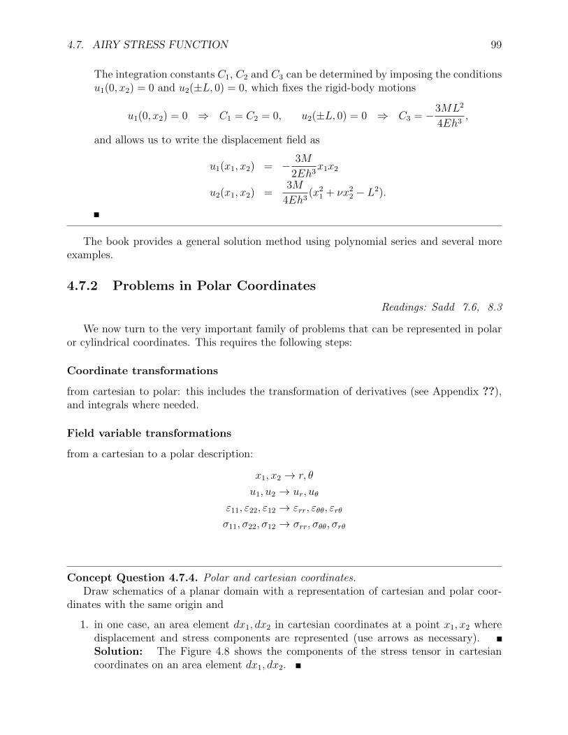
Concept Question 4.7.4. Polar and cartesian coordinates.Draw schematics of a planar domain with a representation of cartesian and polar coor-

dinates with the same origin and

1. in one case, an area element dx1, dx2 in cartesian coordinates at a point x1, x2 wheredisplacement and stress components are represented (use arrows as necessary).Solution: The Figure 4.8 shows the components of the stress tensor in cartesiancoordinates on an area element dx1, dx2.




2. in the other case, an area element dr, rdθ in polar coordinates at a point r, θ whichrepresents the same location as before where polar displacement and stress componentsare represented (use arrows as necessary). Solution: The Figure 4.9 shows thecomponents of the stress tensor in polar coordinates on an area element dr, rdθ.

b

(x1, x2)

e1

e2

dx1

dx2

σ11

σ22

σ21

σ12

Figure 4.8: Stress components on an area element cartesian coordinates.

b

(r, θ)

e1

e2

dr

rdθ

σrr

σrθ

σθθ

σθr

Figure 4.9: Stress components on an area in polar coordinates.

Transformation of the governing equations to polar coordinates

The book provides a general and comprehensive derivation of the relevant expressions. Thederivations of the strain-displacement relations and stress equilibrium equations in polarcoordinates are given in the Appendix ??. The constitutive laws do not change in polarcoordinates if the material is isotropic, as the coordinate transformation at any point is arotation from one to another orthogonal coordinate systems.

Here, we derive the additional expressions needed.


Biharmonic operator in polar coordinates In cartesian coordinates: φ = φ(x, y).

∇4φ = ∇2∇2φ =

(∂2

∂x2+

∂2

∂y2

)(∂2φ

∂x2+∂2φ

∂y2

)(4.42)

= φ,xxxx + 2φ,xxyy + φ,yyyy (4.43)

We seek to express φ as a function of r, θ, i.e. φ = φ(r, θ) and its corresponding ∇4φ(r, θ)upon a transformation to polar coordinates:

r =√x2 + y2, θ = tan−1

(yx

)How to replace first cartesian derivatives with expressions in polar coordinates:start by using the chain rule to relate the partial derivatives of φ in their cartesian and polardescriptions:

∂φ(x, y)

∂x=∂φ(r, θ)

∂r

∂r

∂x+∂φ(r, θ)

∂θ

∂θ

∂x(4.44)

∂φ(x, y)

∂y=∂φ(r, θ)

∂r

∂r

∂y+∂φ(r, θ)

∂θ

∂θ

∂y(4.45)

(4.46)

The underlined factors are the components of the Jacobian of the transformation betweencoordinate systems:

∂r

∂x=

∂

∂x

√x2 + y2 =

1

2

1√x2 + y2

2x =x

r= cos θ (4.47)

∂r

∂y=y

r= sin θ (4.48)

∂θ

∂x=

∂

∂x

(tan−1

(yx

))=

1

1 +(yx

)2

(−yx2

)=

−yx2 + y2

= −sin θ

r(4.49)

∂θ

∂y=

1

1 +(yx

)2

(1

x

)=

x

r2=

cos θ

r(4.50)

∂φ

∂x=∂φ

∂rcos θ +

∂φ

∂θ

(− sin θ

r

)(4.51)

∂φ

∂y=∂φ

∂rsin θ +

∂φ

∂θ

(cos θ

r

)(4.52)

How to replace second cartesian derivatives with expressions in polar coordi-nates:

∂2φ

∂x2=

[∂()

∂rcos θ − sin θ

r

∂()

∂θ

] [∂φ


r

∂φ

∂θ

]=

φ,rr cos2 θ − sin θ cos θ

rφ,rθ +

sin θ cos θ

r2φ,θ −

sin θ cos θ

rφ,rθ+

sin2 θ

rφ,r +

1

r2sin θ (cos θφ,θ + sin θφ,θθ) (4.53)


∂2φ

∂y2=

[∂()

∂rsin θ +

∂()

∂θ

cos θ

r

] [∂φ

∂rsin θ +

∂φ

∂θ

cos θ

r

]=

φ,rr sin2 θ +sin θ cos θ

rφ,rθ −

sin θ cos θ

r2φ,θ +

sin θ cos θ

rφ,rθ+

cos2 θ

rφ,r +

cos2 θ

r2φ,θθ −

sin θ cos θ

r2φ,θ (4.54)

Obtain an expression for the Laplacian in polar coordinates by adding up thesecond derivatives:

φ,xx + φ,yy = (cos2 θ + sin2 θ)︸︷︷︸=1

φ,rr + (−2 + 2)︸︷︷︸=0

sin θ cos θ

rφ,rθ + (2− 2)︸︷︷︸

=0

sin θ cos θ

r2φ,θ+

=1︷︸︸︷(cos2 θ + sin2 θ)

rφ,r +

=1︷︸︸︷(cos2 θ + sin2 θ)

r2φ,θθ (4.55)

The Laplacian can then be written as:

∇2φ = φ,xx + φ,yy = φ,rr +1

rφ,r +

1

r2φ,θθ (4.56)

In general:

∇2() = (),xx + (),yy = (),rr +1

r(),r +

1

r2(),θθ (4.57)

This allows us to write the biharmonic operator as:

∇4φ = ∇2(∇2φ) =

[(),rr +

1

r(),r +

1

r2(),θθ

] [φ,rr +

1

rφ,r +

1

r2φ,θθ

](4.58)

In general, it is not necessary to expand this expression.Expressions for the polar stress components: σrr, σθθ, σrθ can be obtained by notic-

ing that any point can be considered as the origin of the x-axis, so that:

σrr = σxx

∣∣∣θ=0

=∂2φ

∂y2

∣∣∣θ=0

=1

r

∂φ

∂r+

1

r2

∂2φ

∂θ2→ σrr =

1

rφ,r +

1

r2φ,θθ (4.59)

σθθ = σyy

∣∣∣θ=0

=∂2φ

∂x2

∣∣∣θ=0

=∂2φ

∂r2→ σθθ = φ,rr (4.60)

To obtain σrθ = σxy

∣∣∣θ=0

= − ∂2φ∂x∂y

∣∣∣θ=0

, we need to evaluate φ,xy in polar coordinates:

∂

∂x

(∂φ

∂y

)=

[∂()


r

∂()

∂θ

] [∂φ

∂rsin θ +

∂φ

∂θ

cos θ

r

]= φ,rr sin θ cos θ+

cos2 θ

r

(φ,rθ −

1

rφ,θ

)−sin θ

r(φ,rθ sin θ+φ,r cos θ)−sin θ

r2(φ,θθ cos θ−φ,θ sin θ)

(4.61)


σrθ = −φ,rθ1

r+ φ,θ

1

r2(4.62)

Verify differential equations of stress equilibrium

The differential equations of stress equilibrium in polar coordinates are (see Appendix ??):

σrr,r +1

rσrθ,θ +

σrr − σθθr

= 0 (4.63)

1

rσθθ,θ + σrθ,r +

2σrθr

= 0 (4.64)

Verification:

σrr,r =

(1

rφ,r +

1

r2φ,θθ

),r

= − 1

r2φ,r+

1

rφ,rr−

2

r3φ,θθ+

1

r2φ,θθr

1

rσrθ,θ =

1

r

(−φ,rθ

1

r+ φ,θ

1

r2

),θ

= −φ,rθθ1

r2+φ,θθ

1

r3

σrr − σθθr

=1

r

(1

rφ,r +

1

r2φ,θθ

)− 1

rφ,rr =

1

r2φ,r+

1

r3φ,θθ−

1

rφ,rr

Adding the the left and right hand sides we note that all terms on the right with like colorscancel out and the first equilibrium equation in polar coordinates is satisfied.

Applying the same procedure to the second equilibrium equation in polar coordinates,(4.64):

1

rσθθ =

1

r(φ,rr),θ =

1

rφ,rrθ

σrθ,r =

(−φ,rθ

1

r+ φ,θ

1

r2

),r

= −φ,rrθ1

r+φ,rθ

1

r2+φ,rθ

1

r2− 2

r3φ,θ

2σrθr

= −φ,rθ2

r2+φ,θ

2

r3

we note that all terms on the right with like colors cancel out and the second equilibriumequation in polar coordinates is satisfied.

We now consider problems with symmetry with respect to the z-axis.

4.7.3 Axisymmetric stress distribution

In this case, there cannot be any dependence of the field variables on θ and all derivativeswith respect to θ should vanish. In addition, σrθ = 0 by symmetry (i.e. because of theindependence on θ σrθ could only be constant, but that would violate equilibrium). Thenthe second equilibrium equation is identically 0. The first equation becomes (body forcesignored):

dσrrdr

+σrr − σθθ

r= 0 (4.65)


The biharmonic equation becomes: (d2

dr2+

1

r

d

dr

)(d2φ

dr2+

1

r

dφ

dr

)= 0

φIV +

(− 1

r2φ′ − 1

rφ′′)

+1

rφ′′′ +

1

r

(− 1

r2φ′ +

1

rφ′′)

= 0

φIV +2

r3φ′− 1

r2φ′′− 1

r2φ′′+

1

rφ′′′+

1

rφ′′′− 1

r3φ′+

1

r2φ′′ = 0

φIV +2

rφ′′′ − 1

r2φ′′ +

1

r3φ′ = 0 (4.66)

We obtain a single ordinary differential equation for φ(r) with variable coefficients. The gen-eral solution may be obtained by first reducing the equation to one with constant coefficientsby making the substitution r = et, r′(t) = et, t = log r, t′(r) = 1

r= e−t

φ′(r) = φ′(t)t′(r) = φ′(t)e−t, ()′(r) = ()′(t)e−t

φ′′(r) =(φ′(t)e−t

)′(t)e−t = e−2t (−φ′(t) + φ′′(t))

φ′′′(r) =[e−2t (−φ′(t) + φ′′(t))

]′(t)e−t = e−3t (2φ′(t)− 3φ′′(t) + φ′′′(t))

φIV (r) = e−3t(−6φ′(t) + 11φ′′(t)− 6φ′′′(t) + φIV (t)

)Multiply equation (4.66) by r4 and replace these results to obtain::

r4φIV + 2r3φ′′′ − r2φ′′ + rφ = φIV (t)− 4φ′′′(t) + 4φ′′(t) = 0 (4.67)

To solve this, assume φ = ert, φ′ = rert = rφ, φ′′ = r2φ, φ′′′ = r3φ, φIV = r4φ. Then:

(r4 − 4r3 + 4r2)ert = 0 ⇐⇒ r2(r2 − 4r + 4) = 0 (4.68)

The roots of this equation are: r = 0, r = 2 (both double roots), then:

φ = C1 + C2t+ C3e2t + C4te

2t

Replace t = log r

φ(r) = C1 + C2 log r + C3r2 + C4r

2 log r (4.69)

The stresses follow from:

σrr =1

rφ,r =

C2

r2+ 2C3 + C4(2 log r + 1) (4.70)

σθθ = φ,rr = −C2

r2+ 2C3 + C4(2 log r + 3) (4.71)

This constitutes the most general stress field for axisymmetric problems. We will now con-sider examples of application of this general solution to specific problems. This involvesapplying the particular boundary conditions of the case under consideration in terms ofapplied boundary loadings at specific locations (radii) including load free boundaries.


Concept Question 4.7.5. The boring case: Consider the case where there is no hole atthe origin. Use the general stress solution to show that the only possible solution (assumingthere are no body forces) is a state of uniform state σθθ = σrr = constant. Solution: Ifthere is no hole, r = 0 is part of the domain and according to the general solution (4.70) thestresses go to∞ at that location unless C2 = C4 = 0. In this case, the only possible solution(if there’s no body forces) is a constant state σrr = σθθ = 2C3.

Concept Question 4.7.6. A counterexample (well, not really): no hole but bodyforces The compressor disks in a Rolls-Royce RB211-535E4B triple-shaft turbofan used in

Figure 4.10: Cut-away of a Rolls-Royce RB211-535E4B triple-shaft turbofan used in B-757’s(left) and detail of intermediate pressure compressor stages (right)

B-757’s have a diameter D = 0.7m and are made of a metallic alloy with mass densityρ = 6500kg · m−3, Young’s modulus E = 500GPa, Poisson ratio ν = 0.3 and yield stressσ0 = 600MPa.

1. Compute the maximum turbine rotation velocity at which the material first yieldsplastically (ignore the effect of the blades).

2. Estimate the minimum clearance between the blade tips and the encasing required toprevent contact.

Solution: The centripetal acceleration −ω2r acts in the radial direction and appearsin the stress equilibrium equation in the radial direction as an inertia term

∂σrr∂r

+σrr − σθθ

r= ρar = −ρω2r, or:

r∂σrr∂r

+ σrr − σrθ + ρω2r2 = 0


Due to axial symmetry, σrθ = 0 everywhere and the equation of equilibrium in the circum-ferential direction gives that ∂σθθ

∂θ= 0, σθθ = σθθ(r) (This actually assumes constant angular

velocity, why?)Since the radial equilibrium equation involves two unknowns, the problem cannot be

solved from equilibrium considerations exclusively (statically indeterminate). The approachsought is to obtain a Navier equation involving the radial displacement as the only unknown.For this we will need to consider the strain-displacement and constitutive relations.

The strain-displacement relations in this case reduce to:

εrr =durdr

, εθθ =urr

We will assume plane stress conditions for each disk. In this case, the constitutive lawcan be written as:

σrr =E

1− ν2(εrr + νεθθ)

σθθ =E

1− ν2(εθθ + νεrr)

Combining them, we obtain:

σrr =E

1− ν2

(durdr

+ νurr

)σθθ =

E

1− ν2

(urr

+ νdurdr

)which replaced in the equilibrium equation gives the following ordinary differential equationfor the radial displacement:

r2ur,rr + rur,r − ur +1− ν2

Eρω2r3 = 0.

The general solution of this equation is (details discussed separately):

ur = C1r +C2

r− 1− ν2

8EρΩ2r3 (4.72)

The stresses follow as:

σrr =E

1− ν2

(durdr

+ νurr

)=

E

1− νC1 −

E

1 + ν

C2

r2− 3 + ν

8ρω2r2

σθθ =E

1− ν2

(urr

+ νdurdr

)=

E

1− νC1 +

E

1 + ν

C2

r2− 1 + 3ν

8ρω2r2


Application of boundary conditions: We know that the displacement at r = 0cannot go to ∞ (in fact, we expect it to be zero). This implies C2 = 0. The stresses on theouter boundary at r = R (ignoring the blades) should go to zero:

σrr(r = R) = 0 =E

1− νC1 −

3 + ν

8ρω2R2

⇒ C1 =(1− ν)(3 + ν)

8Eρω2R2

The radial displacement is then given by

ur(r) =1− ν8E

ρω2r[(3 + ν)R2 − (1 + ν)r2

]and the dimensionless radial and hoop stresses are:

σrrρω2R2

=3 + ν

8

[1− r2

]σθθ

ρω2R2=

3 + ν

8

[1− 1 + 3ν

3 + νr2

]where r = r/R. Both stress components are maximum at r = 0. According to the vonMises criterion (to be discussed later in the class), the material will yield when the followingcombination of stress components or effective stress σeff reaches the yield stress:

σeff =1√2

√(σrr − σθθ)2 + σ2

θθ + σ2rr

=ρω2R2

8

√(7ν2 + 2ν + 7)r4 − 4(1 + ν)(3 + ν)r2 + (3 + ν)2 ≤ σy

The maximum effective stress is achieved at r = 0 and its value:

σeffmax =3 + ν

8ρω2R2

must be less than the yield stress. From this, we obtain the maximum angular velocity:

ωmax =

√8σy

(3 + ν)ρR2

In order to estimate the necessary clearance, we need to compute the radial displacementat r = R for ωmax:

umax(r = R) = 2(1− ν)

ν + 3

σyER

Replacing the values for the problem we obtain:

ωmax = 675 · s−1 ∼ 6450rpm


This is somewhat low for a modern turbine, where angular velocities of ∼ 10000rpms arecommon. What strategies would you consider to solve this problem?

The displacement at r = R is:

umax = 0.35 · 10−3m

about a third of a millimeter.

Now let’s get back to the general solution and apply it to other problems of interest. Weneed to have a hole at r = 0 so that other solutions are possible.

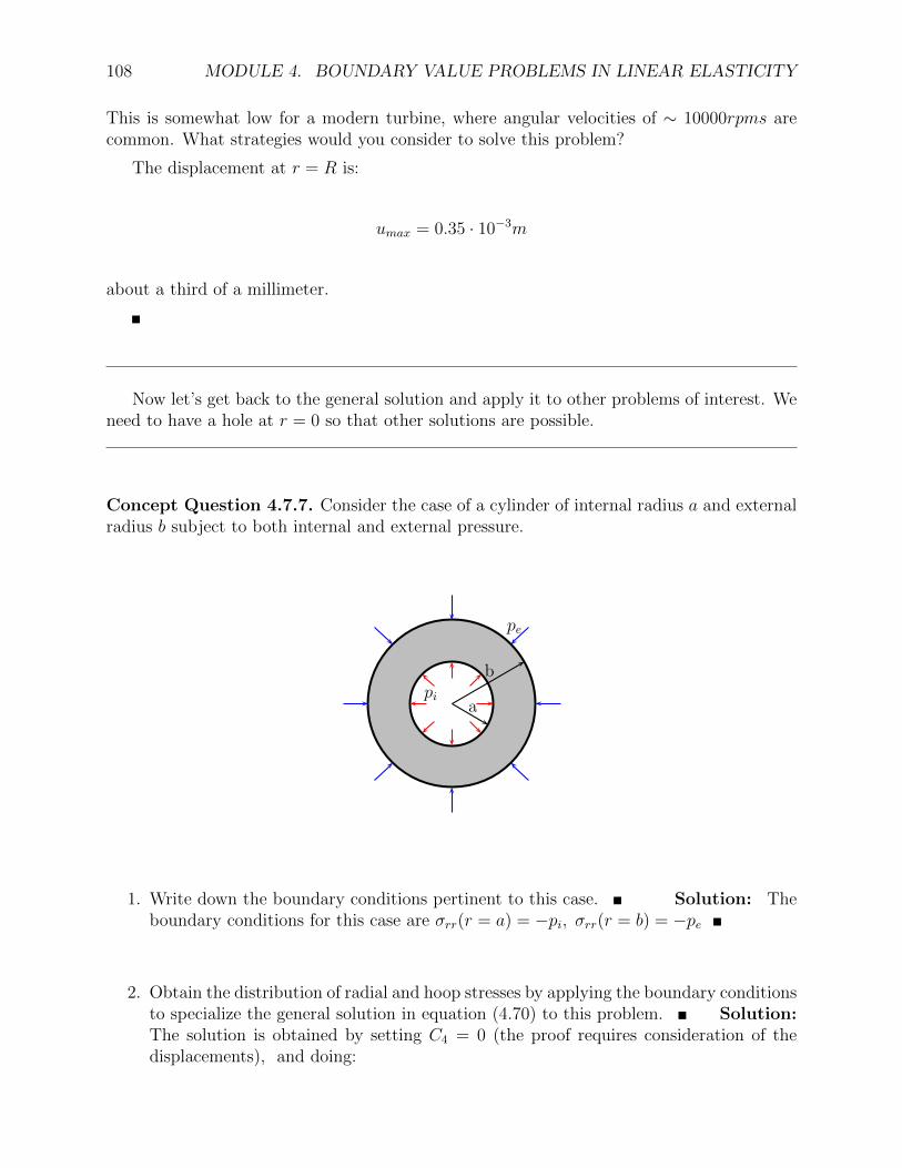
Concept Question 4.7.7. Consider the case of a cylinder of internal radius a and externalradius b subject to both internal and external pressure.

b

a

pe

pi

1. Write down the boundary conditions pertinent to this case. Solution: Theboundary conditions for this case are σrr(r = a) = −pi, σrr(r = b) = −pe

2. Obtain the distribution of radial and hoop stresses by applying the boundary conditionsto specialize the general solution in equation (4.70) to this problem. Solution:The solution is obtained by setting C4 = 0 (the proof requires consideration of thedisplacements), and doing:


σrr(r = a) = −pi =C2

a2+ 2C3

σrr(r = b) = −pe =C2

b2+ 2C3

⇒ pe − pi =

(1

a2− 1

b2

)C2, ⇒ C2 =

a2b2

b2 − a2(pe − pi)

1

2(−peb2 + pia

2) = (b2 − a2)C3, ⇒ C3 =(pia

2 − peb2)

2(b2 − a2)

σrr(r) = 2C3 +C2

r2

σrr(r) =pia

2 − peb2

b2 − a2+a2b2(pe − pi)r2(b2 − a2)

σθθ(r) = 2C3 −C2

r2

σθθ(r) =pia

2 − peb2

b2 − a2− a2b2(pe − pi)

r2(b2 − a2)

3. How does the solution for the stresses depend on the elastic properties of the material?Solution: As expected from the biharmonic equation for no body forces, the

stresses in the plane do not depend on the elastic constants.

4. How would the solution change for plane strain conditions? Solution: Asa consequence, the stresses in the plane do not change whether we are in plane stressor strain. However, the out-of-plane stress σ33 is of course zero in plane stress and inplane strain it would be

σ33 = ν(σrr + σθθ) = 2νpia

2 − peb2

b2 − a2= constant!!

5. Sketch the solution σrr(r) and σθθ(r) normalized with pi for pe = 0 and b/a = 2/1 andverify your intuition on the stress field distribution Solution:

As can be seen from the figure, the maximum


stresses happen at the inner radius and decrease toward the boundary. The radialcomponent vanishes at the outer boundary as it should, but the hoop stress does not.

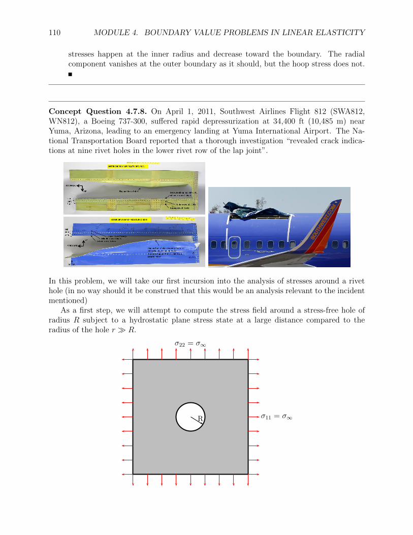
Concept Question 4.7.8. On April 1, 2011, Southwest Airlines Flight 812 (SWA812,WN812), a Boeing 737-300, suffered rapid depressurization at 34,400 ft (10,485 m) nearYuma, Arizona, leading to an emergency landing at Yuma International Airport. The Na-tional Transportation Board reported that a thorough investigation “revealed crack indica-tions at nine rivet holes in the lower rivet row of the lap joint”.

In this problem, we will take our first incursion into the analysis of stresses around a rivethole (in no way should it be construed that this would be an analysis relevant to the incidentmentioned)

As a first step, we will attempt to compute the stress field around a stress-free hole ofradius R subject to a hydrostatic plane stress state at a large distance compared to theradius of the hole r R.

Rσ11 = σ∞

σ22 = σ∞


1. Write down the boundary conditions pertinent to this case. Solution: Theboundary conditions for this case are σrr(r →∞) = σ∞, σrr(r = R) = 0

2. Obtain the distribution of radial and hoop stresses by applying the boundary conditionsto specialize the general solution in equation (4.70) to this problem. Solution:The general solution supports finite stresses at r → ∞ for C4 = 0 and C2, C3 6= 0.Applying the first boundary condition:

σrr(r →∞) = σ∞ = 2C3, → C3 =1

2σ∞

Applying the second boundary condition:

0 =C2

R2+ σ∞, → C2 = −R2σ∞

and the solution is:

σrr = σ∞

[1−

(R

r

)2]

(4.73)

σθθ = σ∞

[1 +

(R

r

)2]

(4.74)

3. Compute the maximum hoop stress and its location. What is the stress concentrationfactor for this type of remote loading on the hole? Solution: Clearly, themaximum hoop stress take place at r = R and its value is:

σmaxθθ = 2σ∞

The next step is to look at the case of asymmetric loading, e.g. remote uniform loadingin one direction, say σ11(r → ∞) = σ∞. The main issue we have is that this case does notcorrespond to axisymmetric loading. It turns out, the formulation in polar coordinates stillproves advantageous in this case.

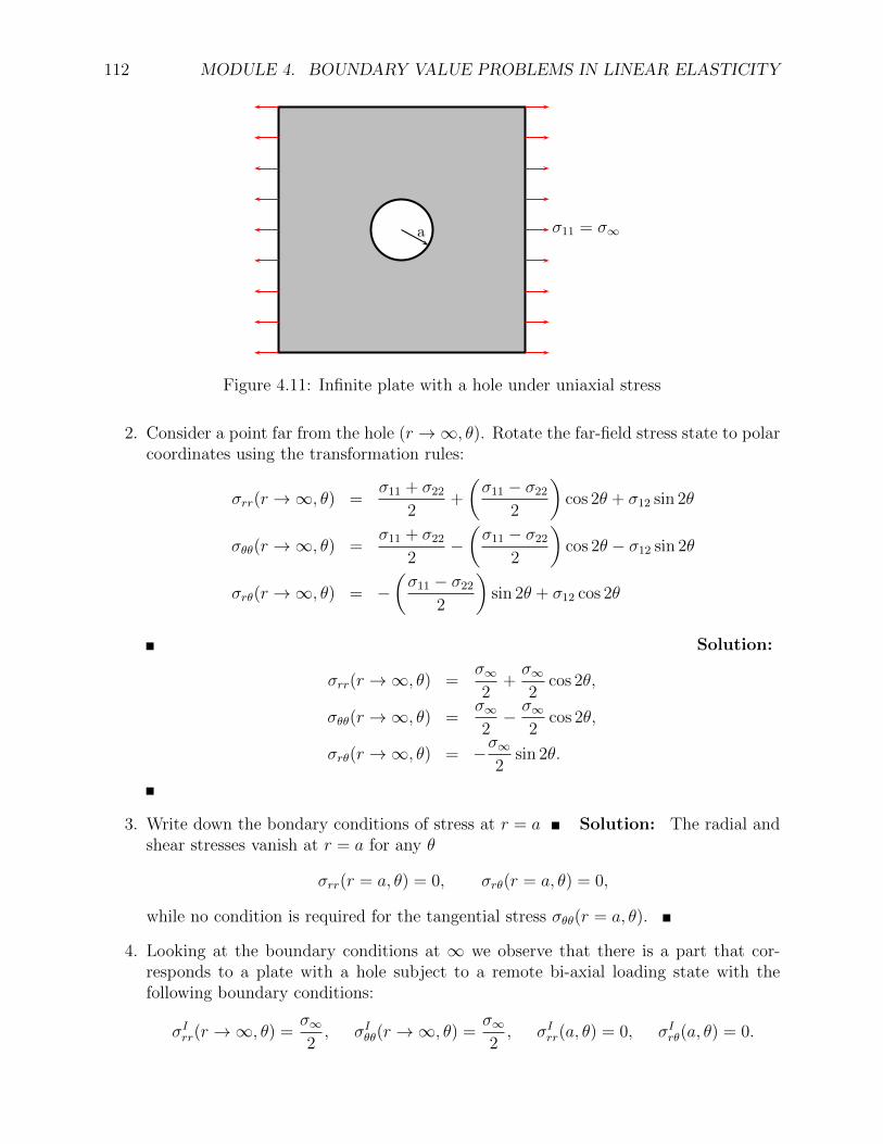
Concept Question 4.7.9. Infinite plate with a hole under uniaxial stress.Consider an infinite plate with a small hole of radius a as shown in Figure 4.7.9. The

goal is to determine the stress field around the whole.

1. Write the boundary conditions far from the hole in cartesian coordinates Solution:

σ11(x1 →∞, x2) = σ∞, σ22(x1 →∞, x2) = 0, σ12(x2 →∞, x2) = 0.


a σ11 = σ∞

Figure 4.11: Infinite plate with a hole under uniaxial stress

2. Consider a point far from the hole (r →∞, θ). Rotate the far-field stress state to polarcoordinates using the transformation rules:

σrr(r →∞, θ) =σ11 + σ22

2+

(σ11 − σ22

2

)cos 2θ + σ12 sin 2θ

σθθ(r →∞, θ) =σ11 + σ22

2−(σ11 − σ22

2

)cos 2θ − σ12 sin 2θ

σrθ(r →∞, θ) = −(σ11 − σ22

2

)sin 2θ + σ12 cos 2θ

Solution:

σrr(r →∞, θ) =σ∞2

+σ∞2

cos 2θ,

σθθ(r →∞, θ) =σ∞2− σ∞

2cos 2θ,

σrθ(r →∞, θ) = −σ∞2

sin 2θ.

3. Write down the bondary conditions of stress at r = a Solution: The radial andshear stresses vanish at r = a for any θ

σrr(r = a, θ) = 0, σrθ(r = a, θ) = 0,

while no condition is required for the tangential stress σθθ(r = a, θ).

4. Looking at the boundary conditions at ∞ we observe that there is a part that cor-responds to a plate with a hole subject to a remote bi-axial loading state with thefollowing boundary conditions:

σIrr(r →∞, θ) =σ∞2, σIθθ(r →∞, θ) =

σ∞2, σIrr(a, θ) = 0, σIrθ(a, θ) = 0.


Write down the solution for this problem: Solution: From the previous problem:

σIrr(r, θ) =σ∞2

[1− a2

r2

]σIθθ(r, θ) =

σ∞2

[1 +

a2

r2

]σIrθ(r, θ) = 0.

5. The second part is not axisymmetric and therefore more involved, as we need to solvethe homogeneous biharmonic equation in polar coordinates:

∇4φ =∂4φ

∂r4+

2

r2

∂4φ

∂r2∂θ2+

1

r4

∂4φ

∂θ4+

2

r

∂3φ

∂r3− 2

r3

∂3φ

∂r∂θ2− 1

r2

∂2φ

∂r2+

4

r4

∂2φ

∂θ2+

1

r3

∂φ

∂r.

Due to the periodicity in θ the problem is greatly simplified and we can assume asolution of the form:

φ(r, θ) = f(r) cos 2θ

Replace this form of the solution in the biharmonic equation to obtain the following:

∇4φ =

(f IV +

2

rf ′′′ − 9

r2f ′′ +

9

r3f ′)

cos 2θ = 0.

Solution: As this expression is valid for any value of θ, the ODE inparentheses must vanish

f IV +2

rf ′′′ − 9

r2f ′′ +

9

r3f ′ = 0

6. Obtain the solution for this ODE by first converting it to constant coefficients viathe substitution r = et and then using the method of undetermined coefficients whichstarts by assuming a solution of the form f(t) = eαt. Finally, replace t = log r toobtain the final solution to the variable coefficient ODE. The result should be:

f(r) = C1 + C2r2 + C3r

4 + C4/r2.

Solution:

7. From the resulting Airy’s stress function

φ(r, θ) = f(r) cos 2θ =

(C1 + C2r

2 + C3r4 +

C4

r2

)cos 2θ.


Write the expressions for the radial, shear, and circumferential components of the stressfield for the second part of the problem (II) using the definitions:

σIIrr (r, θ) =1

r

∂φ

∂r+

1

r2

∂2φ

∂θ2

σIIθθ (r, θ) =∂2φ

∂r2

σIIrθ (r, θ) =1

r2

∂φ

∂θ− 1

r

∂2φ

∂r∂θ.

Solution:

σIIrr (r, θ) = −(

2C2 + 4C1

r2+ 6

C4

r4

)cos 2θ,

σIIθθ (r, θ) =

(2C2 + 12C3r

2 + 6C4

r4

)cos 2θ,

σIIrθ (r, θ) =

(2C2 + 6C3r

2 − 2C1

r2− 6

C4

r4

)sin 2θ.

8. Use the boundary conditions at ∞ for the second part of the problem to obtain thevalues of the constants. The following results should be obtained C3 = 0 and C2 =−σ∞/4, C1 = σ∞a

2/2 and C4 = −σ∞a4/4: Solution:

The shear boundary condition is: σIIrθ (r → ∞, θ) = −σ∞2

sin 2θ, which gives C3 = 0and C2 = −σ∞/4.

In addition, the boundary conditions σIIrr (a, θ) = 0 and σIIrθ (a, θ) = 0 give:

2C2 + 4C1

a2+ 6

C4

a4= 0, 2C2 − 2

C1

a2− 6

C4

a4= 0,

which gives the values sought.

9. Replace the values of the constants to obtain the expressions for the stress field for thesecond part of the problem:

σrr(r, θ) =σ∞2

(1− 4

a2

r2+ 3

a4

r4

)cos 2θ,

σθθ(r, θ) = −σ∞2

(1 + 3

a4

r4

)cos 2θ,

σrθ(r, θ) =σ∞2

(−1− 2

a2

r2+ 3

a4

r4

)sin 2θ.

Solution:


Finally, we can add the solutions to problems (I) and (II) and obtain the completestress field:

σrr(r, θ) =σ∞2

[(1− a2

r2

)+

(1− 4

a2

r2+ 3

a4

r4

)cos 2θ

],

σθθ(r, θ) =σ∞2

[(1 +

a2

r2

)−(

1 + 3a4

r4

)cos 2θ

],

σrθ(r, θ) =σ∞2

[−1− 2

a2

r2+ 3

a4

r4

]sin 2θ .

10. Sketch the plot of σθθ(a, θ) to obtain the stress concentration factor of the hoop stressaround the hole. Solution: The hoop stress is illustrated in Figure 4.12.

Figure 4.12: Stress concentration: infinite plate with a central hole subject to uniaxial stress.

Documents

Module 4 Boundary value problems in linear elasticityweb.mit.edu/16.20/homepage/4_ElasticityBVP/ElasticityBVP_files/... · Module 4 Boundary value problems in linear elasticity Learning