Embed Size (px)
Citation preview

Module 7: Dictionaries via Hashing
CS 240 – Data Structures and Data Management
T. Biedl K. Lanctot M. Sepehri S. WildBased on lecture notes by many previous cs240 instructors
David R. Cheriton School of Computer Science, University of Waterloo
Winter 2018
References: Sedgewick 12.2, 14.1-4
version 2018-03-07 14:23
Biedl, Lanctot, Sepehri, Wild (SCS, UW) CS240 – Module 7 Winter 2018 1 / 23

Outline
1 Dictionaries via HashingHashing IntroductionSeparate ChainingOpen AddressingHash Function Strategies
Biedl, Lanctot, Sepehri, Wild (SCS, UW) CS240 – Module 7 Winter 2018

Outline
1 Dictionaries via HashingHashing IntroductionSeparate ChainingOpen AddressingHash Function Strategies
Biedl, Lanctot, Sepehri, Wild (SCS, UW) CS240 – Module 7 Winter 2018

Lower bound for search
The fastest implementations of the dictionary ADT require Θ(log n) timeto search a dictionary containing n items. Is this the best possible?
Theorem: In the comparison model (on the keys),Ω(log n) comparisons are required to search a size-n dictionary.
Proof: Similar to lower bound for sorting.Any algorithm defines a binary decision tree withcomparisons at the nodes and actions at the leaves.There are at least n + 1 different actions (return an item, or “not found”).So there are Ω(n) leaves, and therefore the height is Ω(log n).
Biedl, Lanctot, Sepehri, Wild (SCS, UW) CS240 – Module 7 Winter 2018 2 / 23

Direct AddressingRequirement: For a given M ∈ N,every key k is an integer with 0 ≤ k < M.Data structure: An array A of size M that stores (k, v) via A[k]← v .Example: M = 9, the dictionary stores (2, dog), (6, cat) and (8, pig).
0
1
dog2
3
4
5
cat6
7
pig8
Biedl, Lanctot, Sepehri, Wild (SCS, UW) CS240 – Module 7 Winter 2018 3 / 23

Direct Addressing Runtime
Requirement: For a given M ∈ N,every key k is an integer with 0 ≤ k < M.
Data structure : An array A of size M that stores (k, v) via A[k]← v .
search(k) : Check whether A[k] is emptyinsert(k, v) : A[k]← vdelete(k) : A[k]← empty
Each operation is Θ(1).Total storage is Θ(M).
What sorting algorithm does this remind you of? Counting Sort
Biedl, Lanctot, Sepehri, Wild (SCS, UW) CS240 – Module 7 Winter 2018 4 / 23

Direct Addressing Runtime
Requirement: For a given M ∈ N,every key k is an integer with 0 ≤ k < M.
Data structure : An array A of size M that stores (k, v) via A[k]← v .
search(k) : Check whether A[k] is emptyinsert(k, v) : A[k]← vdelete(k) : A[k]← empty
Each operation is Θ(1).Total storage is Θ(M).
What sorting algorithm does this remind you of?
Counting Sort
Biedl, Lanctot, Sepehri, Wild (SCS, UW) CS240 – Module 7 Winter 2018 4 / 23

Direct Addressing Runtime
Requirement: For a given M ∈ N,every key k is an integer with 0 ≤ k < M.
Data structure : An array A of size M that stores (k, v) via A[k]← v .
search(k) : Check whether A[k] is emptyinsert(k, v) : A[k]← vdelete(k) : A[k]← empty
Each operation is Θ(1).Total storage is Θ(M).
What sorting algorithm does this remind you of? Counting Sort
Biedl, Lanctot, Sepehri, Wild (SCS, UW) CS240 – Module 7 Winter 2018 4 / 23

Hashing
Direct addressing isn’t possible if keys are not integers.And the storage is very wasteful if n M.
Say keys come from some universe U.
Hash function h : U → 0, 1, . . . ,M − 1 maps keys to integers.
Uniform Hashing Assumption: Each hash function value is equally likely.
This depends on the input and how we choose the function (later).
Hash table Dictionary: Array T of size M (the hash table).An item with key k is stored in T [h(k)].
Biedl, Lanctot, Sepehri, Wild (SCS, UW) CS240 – Module 7 Winter 2018 5 / 23

Hashing exampleU = integers, M = 11, h(k) = k mod 11.The hash table stores keys 7, 13, 43, 45, 49, 92. (Values are not shown).
0
451
132
3
924
495
6
77
8
9
4310
Biedl, Lanctot, Sepehri, Wild (SCS, UW) CS240 – Module 7 Winter 2018 6 / 23

Collisions
Generally hash function h is not injective, so many keys can map tothe same integer.
I For example, h(46) = 2 = h(13).We get collisions: we want to insert (k, v) into the table,but T [h(k)] is already occupied.
Two basic strategies to deal with collisions:I Allow multiple items at each table location (buckets)I Allow each item to go into multiple locations (open addressing)
We will evaluate strategies by the average cost of search, insert,delete, in terms of n, M, and/or the load factor α = n/M.
I The example has load factor 611 .
We rebuild the whole hash table and change the value of M when theload factor gets too large or too small.
I This is called rehashing , and costs Θ(M + n).
Biedl, Lanctot, Sepehri, Wild (SCS, UW) CS240 – Module 7 Winter 2018 7 / 23

Outline
1 Dictionaries via HashingHashing IntroductionSeparate ChainingOpen AddressingHash Function Strategies
Biedl, Lanctot, Sepehri, Wild (SCS, UW) CS240 – Module 7 Winter 2018

Separate Chaining
Each table entry is a bucket containing 0 or more KVPs.This could be implemented by any dictionary (even another hash table!).
The simplest approach is to use an unsorted linked list in each bucket.This is called collision resolution by separate chaining .
search(k): Look for key k in the list at T [h(k)].insert(k, v): Add (k, v) to the front of the list at T [h(k)].delete(k): Perform a search, then delete from the linked list.
Biedl, Lanctot, Sepehri, Wild (SCS, UW) CS240 – Module 7 Winter 2018 8 / 23

Chaining example
M = 11, h(k) = k mod 11
insert()
h
0
451
132
3
924
495
6
77
8
9
4310
Biedl, Lanctot, Sepehri, Wild (SCS, UW) CS240 – Module 7 Winter 2018 9 / 23

Chaining example
M = 11, h(k) = k mod 11
insert(41)
h(41) = 8
0
451
132
3
924
495
6
77
8
9
4310
Biedl, Lanctot, Sepehri, Wild (SCS, UW) CS240 – Module 7 Winter 2018 9 / 23

Chaining example
M = 11, h(k) = k mod 11
insert(41)
h(41) = 8
0
451
132
3
924
495
6
77
418
9
4310
Biedl, Lanctot, Sepehri, Wild (SCS, UW) CS240 – Module 7 Winter 2018 9 / 23

Chaining example
M = 11, h(k) = k mod 11
insert(46)
h(46) = 2
0
451
132
3
924
495
6
77
418
9
4310
Biedl, Lanctot, Sepehri, Wild (SCS, UW) CS240 – Module 7 Winter 2018 9 / 23

Chaining example
M = 11, h(k) = k mod 11
insert(46)
h(46) = 2
0
451
462 133
924
495
6
77
418
9
4310
Biedl, Lanctot, Sepehri, Wild (SCS, UW) CS240 – Module 7 Winter 2018 9 / 23

Chaining example
M = 11, h(k) = k mod 11
insert(16)
h(16) = 5
0
451
462 133
924
165 496
77
418
9
4310
Biedl, Lanctot, Sepehri, Wild (SCS, UW) CS240 – Module 7 Winter 2018 9 / 23

Chaining example
M = 11, h(k) = k mod 11
insert(79)
h(79) = 2
0
451
792 46 133
924
165 496
77
418
9
4310
Biedl, Lanctot, Sepehri, Wild (SCS, UW) CS240 – Module 7 Winter 2018 9 / 23

Complexity of chaining
Recall the load factor α = n/M.
Assuming uniform hashing, average bucket size is exactly α.
Analysis of operations:search Θ(1 + α) average-case, Θ(n) worst-caseinsert O(1) worst-case, since we always insert in front.delete Same cost as search: Θ(1 + α) average, Θ(n) worst-case
If we maintain M ∈ Θ(n), then average costs are all O(1).This is typically accomplished by rehashing whenever n < c1M or n > c2M,for some constants c1, c2 with 0 < c1 < c2.
Biedl, Lanctot, Sepehri, Wild (SCS, UW) CS240 – Module 7 Winter 2018 10 / 23

Outline
1 Dictionaries via HashingHashing IntroductionSeparate ChainingOpen AddressingHash Function Strategies
Biedl, Lanctot, Sepehri, Wild (SCS, UW) CS240 – Module 7 Winter 2018

Open addressing
Main idea: Each hash table entry holds only one item,but any key k can go in multiple locations.
search and insert follow a probe sequence of possible locations for key k:〈h(k, 0), h(k, 1), h(k, 2), . . .〉 until an empty spot is found.
delete becomes problematic:Cannot leave an empty spot behind; the next search might otherwisenot go far enough.Idea 1: Move later items in the probe sequence forward.Idea 2: lazy deletion. Mark spot as deleted (rather than empty) andcontinue searching past deleted spots.
Simplest idea: linear probingh(k, i) = (h(k) + i) mod M, for some hash function h.
Biedl, Lanctot, Sepehri, Wild (SCS, UW) CS240 – Module 7 Winter 2018 11 / 23

Linear probing example
M = 11, h(k, i) = (h(k) + i) mod 11.
()
h
0
451
132
3
924
495
6
77
8
9
4310
Biedl, Lanctot, Sepehri, Wild (SCS, UW) CS240 – Module 7 Winter 2018 12 / 23

Linear probing example
M = 11, h(k, i) = (h(k) + i) mod 11.
insert(41)
h(41, 0) = 8
0
451
132
3
924
495
6
77
418
9
4310
Biedl, Lanctot, Sepehri, Wild (SCS, UW) CS240 – Module 7 Winter 2018 12 / 23

Linear probing example
M = 11, h(k, i) = (h(k) + i) mod 11.
insert(84)
h(84, 0) = 7
0
451
132
3
924
495
6
77
418
9
4310
Biedl, Lanctot, Sepehri, Wild (SCS, UW) CS240 – Module 7 Winter 2018 12 / 23
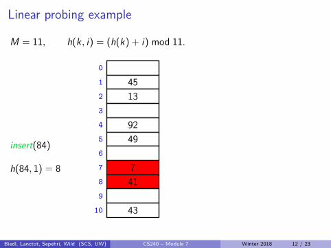
Linear probing example
M = 11, h(k, i) = (h(k) + i) mod 11.
insert(84)
h(84, 1) = 8
0
451
132
3
924
495
6
77
418
9
4310
Biedl, Lanctot, Sepehri, Wild (SCS, UW) CS240 – Module 7 Winter 2018 12 / 23
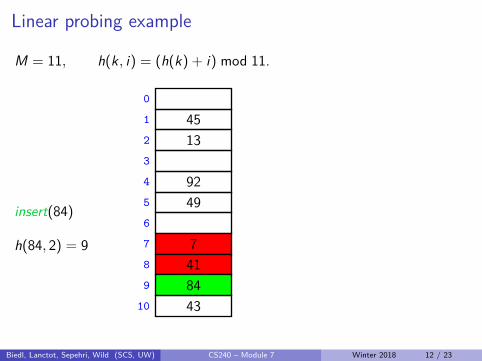
Linear probing example
M = 11, h(k, i) = (h(k) + i) mod 11.
insert(84)
h(84, 2) = 9
0
451
132
3
924
495
6
77
418
849
4310
Biedl, Lanctot, Sepehri, Wild (SCS, UW) CS240 – Module 7 Winter 2018 12 / 23

Linear probing example
M = 11, h(k, i) = (h(k) + i) mod 11.
insert(20)
h(20, 0) = 9
0
451
132
3
924
495
6
77
418
849
4310
Biedl, Lanctot, Sepehri, Wild (SCS, UW) CS240 – Module 7 Winter 2018 12 / 23

Linear probing example
M = 11, h(k, i) = (h(k) + i) mod 11.
insert(20)
h(20, 1) = 10
0
451
132
3
924
495
6
77
418
849
4310
Biedl, Lanctot, Sepehri, Wild (SCS, UW) CS240 – Module 7 Winter 2018 12 / 23
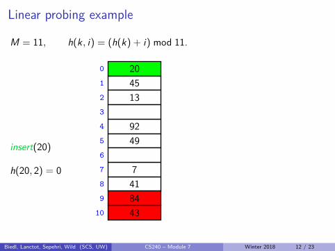
Linear probing example
M = 11, h(k, i) = (h(k) + i) mod 11.
insert(20)
h(20, 2) = 0
200
451
132
3
924
495
6
77
418
849
4310
Biedl, Lanctot, Sepehri, Wild (SCS, UW) CS240 – Module 7 Winter 2018 12 / 23

Linear probing example
M = 11, h(k, i) = (h(k) + i) mod 11.
delete(43)
h(43, 0) = 10
200
451
132
3
924
495
6
77
418
849
deleted10
Biedl, Lanctot, Sepehri, Wild (SCS, UW) CS240 – Module 7 Winter 2018 12 / 23

Linear probing example
M = 11, h(k, i) = (h(k) + i) mod 11.
search(63)
h(63, 0) = 8
200
451
132
3
924
495
6
77
418
849
deleted10
Biedl, Lanctot, Sepehri, Wild (SCS, UW) CS240 – Module 7 Winter 2018 12 / 23

Linear probing example
M = 11, h(k, i) = (h(k) + i) mod 11.
search(63)
h(63, 1) = 9
200
451
132
3
924
495
6
77
418
849
deleted10
Biedl, Lanctot, Sepehri, Wild (SCS, UW) CS240 – Module 7 Winter 2018 12 / 23

Linear probing example
M = 11, h(k, i) = (h(k) + i) mod 11.
search(63)
h(63, 2) = 10
200
451
132
3
924
495
6
77
418
849
deleted10
Biedl, Lanctot, Sepehri, Wild (SCS, UW) CS240 – Module 7 Winter 2018 12 / 23

Linear probing example
M = 11, h(k, i) = (h(k) + i) mod 11.
search(63)
h(63, 3) = 0
200
451
132
3
924
495
6
77
418
849
deleted10
Biedl, Lanctot, Sepehri, Wild (SCS, UW) CS240 – Module 7 Winter 2018 12 / 23

Linear probing example
M = 11, h(k, i) = (h(k) + i) mod 11.
search(63)
h(63, 4) = 1
200
451
132
3
924
495
6
77
418
849
deleted10
Biedl, Lanctot, Sepehri, Wild (SCS, UW) CS240 – Module 7 Winter 2018 12 / 23

Linear probing example
M = 11, h(k, i) = (h(k) + i) mod 11.
search(63)
h(63, 5) = 2
200
451
132
3
924
495
6
77
418
849
deleted10
Biedl, Lanctot, Sepehri, Wild (SCS, UW) CS240 – Module 7 Winter 2018 12 / 23

Linear probing example
M = 11, h(k, i) = (h(k) + i) mod 11.
search(63)
h(63, 6) = 3not found
200
451
132
3
924
495
6
77
418
849
deleted10
Biedl, Lanctot, Sepehri, Wild (SCS, UW) CS240 – Module 7 Winter 2018 12 / 23

Probe sequence operations
probe-sequence-insert(T , (k, v))1. for (j = 0; j < M; j++)2. if T [h(k, j)] is “empty” or “deleted”3. T [h(k, j)] = (k, v)4. return “success”5. return “failure to insert”
probe-sequence-search(T , k)1. for (j = 0; j < M; j++)2. if T [h(k, j)] is “empty”3. return “item not found”4. else if T [h(k, j)] has key k5. return T [h(k, j)]6. // ignore “deleted” and keep searching7. return “item not found”
Biedl, Lanctot, Sepehri, Wild (SCS, UW) CS240 – Module 7 Winter 2018 13 / 23

Double HashingSay we have two hash functions h1, h2 that are independent.
So, under uniform hashing, we assume the probability that a key khas h1(k) = a and h2(k) = b, for any particular a and b, is
1M2 .
For double hashing , define h(k, i) = h1(k) + i · h2(k) mod M whereh2(k) 6= 0 for any k.
search, insert, delete work just like for linear probing,but with this different probe sequence. To get valid probe sequences, we
need gcd(h2(k),M) = 1! Choose M prime.
Biedl, Lanctot, Sepehri, Wild (SCS, UW) CS240 – Module 7 Winter 2018 14 / 23

Double hashing example
M = 11, h1(k) = k mod 11, h2(k) = (bk/2c mod 10) + 1
0
451
132
3
924
495
6
77
8
9
4310
Biedl, Lanctot, Sepehri, Wild (SCS, UW) CS240 – Module 7 Winter 2018 15 / 23

Double hashing example
M = 11, h1(k) = k mod 11, h2(k) = (bk/2c mod 10) + 1
insert(41)
h1(41) = 8
h(41, 0) = 8
0
451
132
3
924
495
6
77
418
9
4310
Biedl, Lanctot, Sepehri, Wild (SCS, UW) CS240 – Module 7 Winter 2018 15 / 23

Double hashing example
M = 11, h1(k) = k mod 11, h2(k) = (bk/2c mod 10) + 1
insert(117)
h1(117) = 7
h(117, 0) = 7
0
451
132
3
924
495
6
77
418
9
4310
Biedl, Lanctot, Sepehri, Wild (SCS, UW) CS240 – Module 7 Winter 2018 15 / 23

Double hashing example
M = 11, h1(k) = k mod 11, h2(k) = (bk/2c mod 10) + 1
insert(117)
h1(117) = 7
h(117, 0) = 7
h2(117) = 9
h(117, 1) = 5
0
451
132
3
924
495
6
77
418
9
4310
Biedl, Lanctot, Sepehri, Wild (SCS, UW) CS240 – Module 7 Winter 2018 15 / 23

Double hashing example
M = 11, h1(k) = k mod 11, h2(k) = (bk/2c mod 10) + 1
insert(117)
h1(117) = 7
h(117, 0) = 7
h2(117) = 9
h(117, 1) = 5
h(117, 2) = 3
0
451
132
1173
924
495
6
77
418
9
4310
Biedl, Lanctot, Sepehri, Wild (SCS, UW) CS240 – Module 7 Winter 2018 15 / 23

Cuckoo hashing
This is a relatively new idea from Pagh and Rodler in 2001.
Again, we use two independent hash functions h1, h2.
Main idea: An item with key k can only be in T [h1(k)] or T [h2(k)].Search and Delete then take constant time.Insert always puts a new item into T [h1(k)].If T [h1(k)] was occupied: “kick out” the other item, which we thenattempt to re-insert into its alternate position.This may lead to a loop of “kicking out”. We detect this by abortingafter too many attempts.In case of failure: rehash with a larger M and new hash functions.
Insert may be slow, but is expected to be constant time if the loadfactor is small enough.
Biedl, Lanctot, Sepehri, Wild (SCS, UW) CS240 – Module 7 Winter 2018 16 / 23
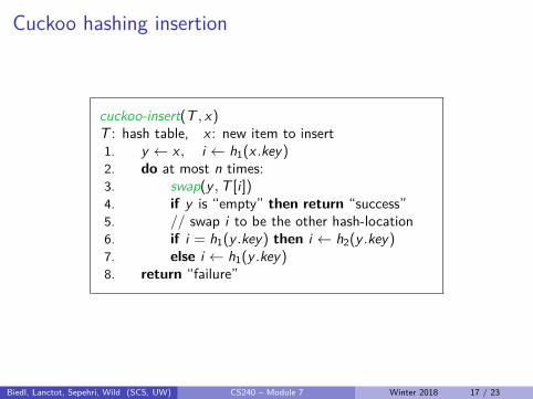
Cuckoo hashing insertion
cuckoo-insert(T , x)T : hash table, x : new item to insert1. y ← x , i ← h1(x .key)2. do at most n times:3. swap(y ,T [i ])4. if y is “empty” then return “success”5. // swap i to be the other hash-location6. if i = h1(y .key) then i ← h2(y .key)7. else i ← h1(y .key)8. return “failure”
Biedl, Lanctot, Sepehri, Wild (SCS, UW) CS240 – Module 7 Winter 2018 17 / 23

Cuckoo hashing example
M = 11, h1(k) = k mod 11, h2(k) = b11(ϕk − bϕkc)c
()
y .key =
h1(y .key) =h2(y .key) =
i =
440
1
2
3
264
5
6
7
8
929
10
Biedl, Lanctot, Sepehri, Wild (SCS, UW) CS240 – Module 7 Winter 2018 18 / 23

Cuckoo hashing example
M = 11, h1(k) = k mod 11, h2(k) = b11(ϕk − bϕkc)c
insert(51)
y .key = 51
h1(y .key) = 7h2(y .key) = 5
i = 7
440
1
2
3
264
5
6
7
8
929
10
Biedl, Lanctot, Sepehri, Wild (SCS, UW) CS240 – Module 7 Winter 2018 18 / 23

Cuckoo hashing example
M = 11, h1(k) = k mod 11, h2(k) = b11(ϕk − bϕkc)c
insert(51)
y .key = 51
h1(y .key) = 7h2(y .key) = 5
i = 7
440
1
2
3
264
5
6
517
8
929
10
Biedl, Lanctot, Sepehri, Wild (SCS, UW) CS240 – Module 7 Winter 2018 18 / 23

Cuckoo hashing example
M = 11, h1(k) = k mod 11, h2(k) = b11(ϕk − bϕkc)c
insert(95)
y .key = 95
h1(y .key) = 7h2(y .key) = 7
i = 7
440
1
2
3
264
5
6
517
8
929
10
Biedl, Lanctot, Sepehri, Wild (SCS, UW) CS240 – Module 7 Winter 2018 18 / 23

Cuckoo hashing example
M = 11, h1(k) = k mod 11, h2(k) = b11(ϕk − bϕkc)c
insert(95)
y .key = 51
h1(y .key) = 7h2(y .key) = 5
i = 5
440
1
2
3
264
5
6
957
8
929
10
51
Biedl, Lanctot, Sepehri, Wild (SCS, UW) CS240 – Module 7 Winter 2018 18 / 23

Cuckoo hashing example
M = 11, h1(k) = k mod 11, h2(k) = b11(ϕk − bϕkc)c
insert(95)
y .key = 51
h1(y .key) = 7h2(y .key) = 5
i = 5
440
1
2
3
264
515
6
957
8
929
10
Biedl, Lanctot, Sepehri, Wild (SCS, UW) CS240 – Module 7 Winter 2018 18 / 23

Cuckoo hashing example
M = 11, h1(k) = k mod 11, h2(k) = b11(ϕk − bϕkc)c
insert(97)
y .key = 97
h1(y .key) = 9h2(y .key) = 10
i = 9
440
1
2
3
264
515
6
957
8
929
10
Biedl, Lanctot, Sepehri, Wild (SCS, UW) CS240 – Module 7 Winter 2018 18 / 23

Cuckoo hashing example
M = 11, h1(k) = k mod 11, h2(k) = b11(ϕk − bϕkc)c
insert(97)
y .key = 92
h1(y .key) = 4h2(y .key) = 9
i = 4
440
1
2
3
264
515
6
957
8
979
10
92
Biedl, Lanctot, Sepehri, Wild (SCS, UW) CS240 – Module 7 Winter 2018 18 / 23

Cuckoo hashing example
M = 11, h1(k) = k mod 11, h2(k) = b11(ϕk − bϕkc)c
insert(97)
y .key = 26
h1(y .key) = 4h2(y .key) = 0
i = 0
440
1
2
3
924
515
6
957
8
979
10
26
Biedl, Lanctot, Sepehri, Wild (SCS, UW) CS240 – Module 7 Winter 2018 18 / 23

Cuckoo hashing example
M = 11, h1(k) = k mod 11, h2(k) = b11(ϕk − bϕkc)c
insert(97)
y .key = 44
h1(y .key) = 0h2(y .key) = 2
i = 2
260
1
2
3
924
515
6
957
8
979
10
44
Biedl, Lanctot, Sepehri, Wild (SCS, UW) CS240 – Module 7 Winter 2018 18 / 23

Cuckoo hashing example
M = 11, h1(k) = k mod 11, h2(k) = b11(ϕk − bϕkc)c
insert(97)
y .key = 44
h1(y .key) = 0h2(y .key) = 2
i = 2
260
1
442
3
924
515
6
957
8
979
10
Biedl, Lanctot, Sepehri, Wild (SCS, UW) CS240 – Module 7 Winter 2018 18 / 23

Cuckoo hashing example
M = 11, h1(k) = k mod 11, h2(k) = b11(ϕk − bϕkc)c
search(26)
y .key =
h1(26) = 4h2(26) = 0
260
1
442
3
924
515
6
957
8
979
10
Biedl, Lanctot, Sepehri, Wild (SCS, UW) CS240 – Module 7 Winter 2018 18 / 23

Cuckoo hashing example
M = 11, h1(k) = k mod 11, h2(k) = b11(ϕk − bϕkc)c
delete(26)
y .key =
h1(26) = 4h2(26) = 0
0
1
442
3
924
515
6
957
8
979
10
Biedl, Lanctot, Sepehri, Wild (SCS, UW) CS240 – Module 7 Winter 2018 18 / 23

Outline
1 Dictionaries via HashingHashing IntroductionSeparate ChainingOpen AddressingHash Function Strategies
Biedl, Lanctot, Sepehri, Wild (SCS, UW) CS240 – Module 7 Winter 2018

Choosing a good hash function
Uniform Hashing Assumption: Each hash function value is equally likely.
Proving is usually impossible, as it requires knowledge ofthe input distribution and the hash function distribution.
We can get good performance by following a few rules.
A good hash function should:be very efficient to computebe unrelated to any possible patterns in the datadepend on all parts of the key
Biedl, Lanctot, Sepehri, Wild (SCS, UW) CS240 – Module 7 Winter 2018 19 / 23

Basic hash functions
If all keys are integers (or can be mapped to integers),the following two approaches tend to work well:
Modular method: h(k) = k mod M.We should choose M to be a prime.
Multiplicative method: h(k) = bM(kA− bkAc)c,for some constant floating-point number A with 0 < A < 1.
Knuth suggests A = ϕ =√5− 12 ≈ 0.618.
Biedl, Lanctot, Sepehri, Wild (SCS, UW) CS240 – Module 7 Winter 2018 20 / 23

Universal Hashing
Every hash functions must fail for some sequences of inputs.Everything hashes to same value. terrible worst case!Rescue: Randomization!
choose a random basic hash function, e.g.
h(k) =((ak + b) mod p
)mod M
for a fixed prime p > M and random numbers a, b ∈ 0, . . . p − 1,a 6= 0.
can prove:for any (fixed) numbers x 6= y , the probability of a collision using arandom h is at most 1
M .
Once again: Can enforce same expected performance for any input as wehad without randomization on average inputs.
Biedl, Lanctot, Sepehri, Wild (SCS, UW) CS240 – Module 7 Winter 2018 21 / 23

Multi-dimensional Data
What if the keys are multi-dimensional, such as strings?
Standard approach is to flatten string w to integer f (w) ∈ N, e.g.
A · P · P · L · E → (65, 80, 80, 76, 69) (ASCII)→ 65R4 + 80R3 + 80R2 + 76R1 + 68R0
(for some radix R, e.g. R = 255)
We combine this with a standard hash functionh : N→ 0, 1, 2, . . . ,M − 1.
With h(f (k)) as the hash values, we then use any standard hash table.
Note: computing each h(f (k)) takes Ω(length of w) time.
Biedl, Lanctot, Sepehri, Wild (SCS, UW) CS240 – Module 7 Winter 2018 22 / 23

Hashing vs. Balanced Search Trees
Advantages of Balanced Search TreesO(log n) worst-case operation costDoes not require any assumptions, special functions,or known properties of input distributionPredictable space usage (exactly n nodes)Never need to rebuild the entire structuresupports ordered dictionary operations (rank, select etc.)
Advantages of Hash TablesO(1) operations (if hashes well-spread and load factor small)We can choose space-time tradeoff via load factorCuckoo hashing achieves O(1) worst-case for search & delete
Biedl, Lanctot, Sepehri, Wild (SCS, UW) CS240 – Module 7 Winter 2018 23 / 23