13 SPEAKER RECOGNITION OVER

TELEPHONE CHANNELS Yu-Hung Kao, Lorin Netsch

and P.K. Rajasekaran

Systems and Information Science Laboratory, Texas Instruments

1 INTRODUCTION

Being able to verify or determine the identity of a person by voice is very useful in many applications. For example, in telephone banking or calling card charging, user identity must be verified before the transaction can be authorized. Most systems use a PIN for authorization, but it can be forgotten or stolen. Other methods of authorization, such as finger prints or retinal scans, may be more secure than a PIN, they are not practical in many situations.

Speaker identification and verification over the telephone is especially important because it has very broad application potential. However, different handsets and transmission channels degrade the signal quality and make the identifica­tion more difficult. The amount of information needed for speaker templates (voice prints) of a large number of subscribers requires large hardware memory resources, data bandwidth and call setup time. We will address these problems in this chapter.

1.1 Definition

We first define the difference between speaker identification and verification:

• Speaker identification: For test speaker x, the task is to determine which one of the n registered speakers the test speaker x is.

299

R. P. Ramachandran et al. (ed .), Modern Methods of Speech Processing© Kluwer Academic Publishers 1995

s

300 CHAPTER 13

• Speaker verification: For test speaker z who claims identity i (i is one of the n registered speakers), the task is a binary decision - accept or reject the claim.

Depending on whether speaker z is one of the n registered speakers or not, the problem is further classified into:

• Closed set: Speaker z is one of the n registered speakers. The system has seen all the speakers and a speaker set specific discriminant can be trained. The closed set task is easier, but not a realistic assumption for many applications.

• Open set: Speaker z is not necessarily one of the n registered speakers. This task is more realistic, especially in speaker verification.

In identification, the rate at which the system incorrectly identifies speakers is used to calibrate system performance. Verification performance is measured using both a plot of Receiver Operating Characteristics (ROC) and the equal error rate. The ROC plot displays the true speaker detection rate (rate at which the system correctly verifies a speaker) versus the impostor acceptance rate (rate at which the system incorrectly verifies an impostor) over a set of decision threshold settings. The equal error rate is defined as the rate at the decision threshold setting where the impostor acceptance rate equals the true speaker rejection rate.

2 CHALLENGES

Speaker identification and verification has been a topic of research for many years [1] [2] [3] [4] [5], and research activities continue to be devoted to the following areas:

2.1 Features

There are two sources of variation among speakers : 1) differences in vocal cords and vocal tract shapes; 2) differences in speaking styles. There are no acoustic cues specifically or exclusively tied to speaker identity. Most of the parameters and features used in speech analysis contain information useful for

Speaker Recognition Over Telephone Channels 301

the identification of both speakers and spoken messages. The effectiveness of features is coupled with distance measures and statistical modeling methods. Good features for identification and verification should: 1) discriminate be­tween speakers whl1e being tolerant of intra-speaker variation; 2) be easy to measure from speech signals; 3) be stable over time; 4) occur frequently and naturally in speech; 5) be channel robust; 6) not be susceptible to mimicry.

In general, spectral features are more effective than prosodic features. Although prosodic features (pitch, stress, speed ... ) are important speaker identity cues for human perception, they have not provided significant performance improve­ments when applied in automatic speaker identification. In addition, prosodic features are susceptible to mimicry.

Sambur [6] examined a total of 92 features, including formant frequencies and bandwidth for vowels, resonances during nasals and fricatives, FO statistics and dynamics, and timing measurements (e.g. formant trajectory slopes in diphthongs, voice-onset time for stops). Using a knock out procedure, he found among the most useful features were F2 in nasals, F2-F3-F4 in vowels, and mean FO.

Spectral coefficients are the most commonly used features [1] [6]. A common measure for effectiveness of individual features is the F-ratio, which compares inter- and intra-speaker feature variances. A larger F -ratio usually indicates better discrimination capability. As long as the feature set covers all the spec­tral contents of the speech signal, the modeling can always take care of the discriminant issues. Typical spectral feature sets found useful are cepstral coefficients (coefficients of the inverse Fourier transform of the log spectrum), principal spectral components, and log area ratios, along with their time deriva­tives.

2.2 Channel and Handset Variation

Channel robustness is a critical issue for real world applications. Telephone signals are affected by handsets, transmission channels, and even speech com­pression algorithms. When training and test conditions are not matched, which is often the case, performance will degrade tremendously [7]. To deal with channel variation, we can either choose features invariant to it [8], design signal processing algorithms to compensate for the variation [9], or build noise models [10].

302 CHAPTER 13

2.3 Free-Text vs. Fixed-Text

Speaker verification often employs a fixed-text mode, where users are required to utter a fixed password. This is useful in cooperative situations. In fixed-text mode, word-specific speaker discriminants can be tuned specifically for speaker variation [11]. Dimensionality reduction and speaker discriminating effects can be achieved because there is no phoneme variation.

In uncooperative situations, such as monitoring a conversation and identifying the speakers, no fixed utterance is available, so the problem becomes free-text. Free-text speaker identification and verification are more difficult than fixed­text because the variation due to different phonemes is much larger than that due to different speakers [1]. Free-text speaker identification must resolve the phoneme variation effect. Work has been done on classification of phonemes before speaker identification [12], which will convert a free-text problem into fixed-text.

2.4 Speaker Modeling

Vector quantization (VQ) [13] and continuous / discrete Hidden Markov Model­ing (HMM) have been compared for speaker identification [14] and no significant difference was observed. The performance strongly depends on VQ code book size or number of HMM mixtures. Larger code book size or more mixtures provide more accurate identification; however, as the code book size or number of mixtures increase performance will eventually saturate. The advantage of HMM is its ability to model temporal information. The result suggests that either temporal information is not very useful for speaker identification or the algorithm is not modeling temporal information correctly. However, if speech recognition is used in the speaker identification / verification algorithm [15], HMM can certainly provide a better time alignment than simply matching the acoustics with the closest VQ codeword. Recently, the idea of cohort compari­son [16] has become popular and provides a method of speaker normalization.

3 TASKS AND CORPORA

In this chapter, we will discuss methods of implementing speaker identifica­tion and verification over telephone channels using VQ and continuous HMM

Speaker Recognition Over Telephone Channels 303

speaker modeling and cohort comparison. We will present results of both free­text and fixed-text experiments applied to a variety of corpora.

Three telephone corpora were used in the experiments presented in this chapter. A fourth corpus was used in fixed-text experiments for additional statistical model training, but not testing.

3.1 King Corpus

The narrowband portion of the King corpus [17] is utilized in free-text identi­fication experiments in this chapter. The corpus was collected in 10 sessions from 51 male speakers, 26 from San Diego and 25 from Nutley. The speak­ers were asked to talk about several topics, so that the speech is natural and spontaneous. The data were collected over long distance telephone lines. The data for the 25 Nutley speakers were much noisier than that of the 26 San Diego speakers. The speech material from each session is approximately 45 seconds long. The data were digitized at 8 kHz and 12-bit resolution. Sessions 1 to 5 and sessions 6 to 10 were collected under different environments. This division of data, known as the great divide, results in serious degradation of performance as observed in [8] when training on one set and testing on the other. We performed our experiments in three contexts: San Diego alone (26 speakers), Nutley alone (25 speakers), and all 51 speakers combined. Further, the experiments were carried out across the great divide producing the most challenging test condition. Because it is a spontaneous monologue corpus, only free-text experiments were performed.

3.2 SPIDRE Corpus

The SPIDRE (SPeaker ID Research and Evaluation) corpus is designed specif­ically for free-text speaker identification experiments. It consists of a set of spontaneous conversations selected from 45 speakers (both male and female) from the SWITCHBOARD corpus [18]. Only the one side of each conversation corresponding to the 45 speakers is used. For each speaker there are four calls and three different handsets were used for these four calls, so two of the four calls are from the same handset. There is no handset overlap between speakers, hence 3 x 45 = 135 handsets were used. The corpus was separated into 4 sets, each set containing one call from each speaker. Sets 1 and 2 are from the same handset, while sets 3 and 4 are from different handsets. In the experiments de­scribed in this chapter, set 1 was used for training, set 2 for the same-channel

304 CHAPTER 13

test, and sets 3 and 4 for cross-channel tests. The statistics from set 1 indicate that the average length of a call is 362 seconds, 35% of which is speech from the desired speaker. Other sets have similar statistics.

3.3 Digit Verification Corpus

The Digit Verification corpus consists of speech from 25 female and 25 male subjects. Each subject provided 25 calls over long-distance telephone lines, and was encouraged to use a wide variety of handsets and environments. During the call, each subject provided three tokens of a unique familiar ten-digit string (a leading digit plus a social security number), and three tokens of the unique digit string of another subject of the same sex.

3.4 Additional Training Corpus

The Additional Training corpus consists of 36 female and 70 male subjects. Each subject provided 25 to 40 calls over long-distance telephone lines, and was encouraged to use a wide variety of handsets and environments. During the call, each subject provided three tokens consisting of a four-digit string and two other non-digit words.

4 FREE-TEXT IDENTIFICATION AND VERIFICATION

This set of experiments used a free-text method for all three corpora. VQ codebooks were used to model the acoustic space of speakers after removal of silence portions of the speech signal.

4.1 Robust Methods

The free-text experiments focused on several methods of robust front-end pro­cessing and cohort comparison. These methods are designed to increase the separability of speakers and reduce channel variation effects.

Speaker Recognition Over Telephone Channels

1

0.9

0.8

0.7

0.6

0.5

0.4

0.3

0.2

0.1

0 0 2

....................... ........

within class variance -inter-class variance --~---

F-ratio ....... .

...............

4 6 8 1.0 12 14 16 18 20 cepstrum index

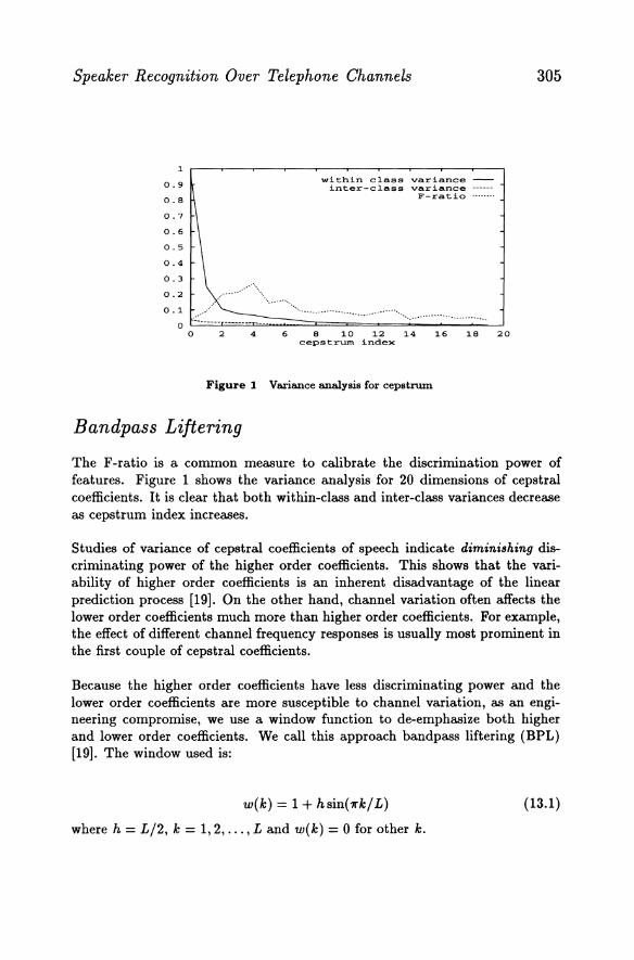
Figure 1 Variance analysis for cepstrum

Bandpass Liftering

305

The F -ratio is a common measure to calibrate the discrimination power of features. Figure 1 shows the variance analysis for 20 dimensions of cepstral coefficients. It is clear that both within-class and inter-class variances decrease as cepstrum index increases.

Studies of variance of cepstral coefficients of speech indicate diminishing dis­criminating power of the higher order coefficients. This shows that the vari­ability of higher order coefficients is an inherent disadvantage of the linear prediction process [19]. On the other hand, channel variation often affects the lower order coefficients much more than higher order coefficients. For example, the effect of different channel frequency responses is usually most prominent in the first couple of cepstral coefficients.

Because the higher order coefficients have less discriminating power and the lower order coefficients are more susceptible to channel variation, as an engi­neering compromise, we use a window function to de-emphasize both higher and lower order coefficients. We call this approach bandpass liftering (BPL) [19]. The window used is:

w(k) = 1 + hsin(7rk/L)

where h = L/2, k = 1,2, ... , Land w(k) = 0 for other k.

(13.1)

306 CHAPTER 13

S(f) ---.~I H(f) --.. ~ S(f) H(f) --....... 1 log(*)

----,.~ log( S(f) ) + log( H(f) ) --....... I RAST A filtering

---.~ log( S(f) )

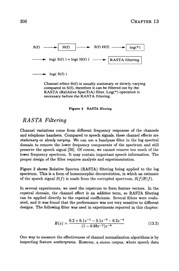
Channel effect H(f) is usually stationary or slowly varying compared to S(f). therefore it can be filtered out by the RAST A (RelAtive SpecTrA) filter. Log(*) operation is necessary before the RAST A filtering.

Figure 2 RASTA filtering

RAS TA Filtering

Channel variations come from different frequency responses of the channels and telephone handsets. Compared to speech signals, these channel effects are stationary or slowly varying. We can use a bandpass filter in the log spectral domain to remove the lower frequency components of the spectrum and still preserve the speech signal [20]. Of course, we cannot remove too much of the lower frequency spectrum. It may contain important speech information. The proper design of the filter requires analysis and experimentation.

Figure 2 shows Relative Spectra (RASTA) filtering being applied to the log spectrum. This is a form of homomorphic deconvolution, in which an estimate of the speech signal S(f) is made from the corrupted spectrum, S(f)H(f).

In several experiments, we used the cepstrum to form feature vectors. In the cepstral domain, the channel effect is an additive term, so RASTA filtering can be applied directly to the cepstral coefficients. Several filters were evalu­ated, and it was found that the performance was not very sensitive to different designs. The following filter was used in experiments reported in this chapter:

H(z) = 0.2 + 0.lz- 1 - 0.lz-3 - 0.2z-4 (1 - 0.98z- 1)z-4

(13.2)

One way to measure the effectiveness of channel normalization algorithms is by inspecting feature scattergrams. However, a stereo corpus, where speech data

Speaker Recognition Over Telephone Channels 307

transmitted through two channels are recorded simultaneously, is required to compute the scattergrams. In our experiments, we used the CSR (Continuous Speech Recognition) corpus, where each utterance is recorded simultaneously by two different microphones (Sennheiser vs. Crown or SONY). Because of the simultaneous recording of two channels, the sample by sample match makes exact comparison of channel effects possible. Here we compare the cepstral coefficients, frame by frame, dimension by dimension.

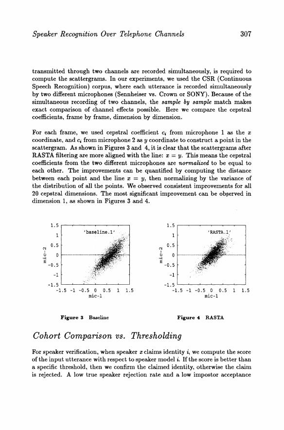
For each frame, we used cepstral coefficient Ci from microphone 1 as the :r;

coordinate, and Ci from microphone 2 as y coordinate to construct a point in the scattergram. As shown in Figures 3 and 4, it is clear that the scattergrams after RASTA filtering are more aligned with the line: :r; = y. This means the cepstral coefficients from the two different microphones are normalized to be equal to each other. The improvements can be quantified by computing the distance between each point and the line :r; = y, then normalizing by the variance of the distribution of all the points. We observed consistent improvements for all 20 cepstral dimensions. The most significant improvement can be obl.!erved in dimension 1, as shown in Figures 3 and 4.

1. 5 r---.--~----r-~-~---,

1

0.5

-1

'baseline.1'

-1. 5 L---'-_""'"""----''__--'-_~__' -1.5 -1 -0.5 0 0.5 1 1.5

mic-1

Figure 3 Baseline

N I

1. 5 r---.--~----r-~-~---,

1

0.5

() 0 1--------.--.,.-'n e

-0.5

-1

-1. 5 L-__'__~_'____'__~__'

-1.5 -1 -0.5 0 0.5 1 1.5 mic-1

Figure 4 RASTA

Cohort Comparison vs. Thresholding

For speaker verification, when speaker z claims identity i, we compute the score of the input utterance with respect to speaker model i. If the score is better than a specific threshold, then we confirm the claimed identity, otherwise the claim is rejected. A low true speaker rejection rate and a low impostor acceptance

308 CHAPTER 13

rate are desired; but as we change the threshold value, trade-off is being made between these two error rates - one decreases, while the other increases.

When we used a threshold as the accept / reject criterion, we were surprised to see that RASTA, which performs so well in our speaker identification ex­periments, actually degraded speaker verification performance. We found that the explanation lies in the difference between absolute threshold vs. cohort comparison.

We inspected the scores of both true speaker attempts and impostor attempts before and after RASTA filtering, and found that the impostor scores improve more than the true speaker scores. In the absolute threshold approach, if true speaker scores and impostor scores improve equally, the performance stays the same. If true speaker scores improve more than impostor scores, the perfor­mance becomes better. However, when impostor scores improve more than true speaker scores, the performance becomes worse. In the speaker identifica­tion experiment, the scores are not compared with an absolute threshold, but compared with peer scores, that is, the score with respect to speaker model i is compared with scores with respect to other speaker models. In this way, the peer scores all depend on the input utterance, and they all adapt together. Uneven improvements are no longer a problem, since they are self-normalized. Following this idea, we changed the verification algorithm from comparing with an absolute threshold to comparing with peer scores. Instead of computing the score of the claimed identity model only, we compute scores with respect to all the registered models. We then determine the rank of the score using the claimed identity model, and subject the rank to a threshold to determine veri­fication acceptance or rejection.

4.2 Free-Text System

The front-end of the system extracted 20 cepstral coefficients from a 14-th order LPC analysis (20 ms frame period, 30 ms window) on speech data sampled at 8KHz. A simple energy threshold was used to discard non-speech. A 3D-element codebook was trained for each speaker as the speaker model. Experiments were performed using cepstral coefficients without (baseline) and with robustness processing. The results were tabulated and compared.

Closed set speaker identification and open set speaker verification were per­formed on all three corpora. For brevity, only selected results are presented here. However, a consistent, significant trend was observed in all experiments.

Speaker Recognition Over Telephone Channels 309

In closed set speaker identification, test utterances were compared frame by frame with each speaker model. The best codeword match was selected for each model, and distortions were accumulated to make the final decision.

For open set speaker verification, half of the speakers in the corpus were used as registered targets, and the other half as impostors. Test utterances were compared with all the registered target models, and the accumulated distortions were tallied to compute the rank of the claimed identity. If the rank was better than a certain threshold, then verification was declared successful; otherwise, the speaker was declared an impostor. The thresholds were adjusted over a range to generate the ROC plot (true speaker detection vs. impostor false alarm).

A closed-set speaker verification experiment was performed using the Digit Verification corpus. This experiment applied the cohort comparison ranking algorithm.

4.3 Results

King Corpus

Free-text, closed set speaker identification results using the King corpus are shown below. Robustness processing shows significant and consistent improve­ments.

The table below shows results within the great divide: we trained on sessions 1, 2, 3, and tested on sessions 4, 5; and trained on sessions 6, 7, 8, and tested on sessions 9, 10.

Identification error rate Front-end San Diego-26 Nutley-25 All-51

Baseline 18.3% 65% 41.2% BPL 14.4% 53% 33.3%

RASTA 8.6% 50% 28.9% BPL + RASTA 5.8% 39% 22.1%

310 CHAPTER 13

Below are results across the great divide: we trained on sessions 1, 2, 3, and tested on sessions 9, 10; and trained on sessions 6, 7, 8, and tested on sessions 4, 5.

Identification error rate Front-end San Diego-26 Nutley-25 All-51

Baseline 92.3% 64% 80.4% BPL 63.5% 54% 63.2%

RASTA 57.7% 47% 56.4% BPL + RASTA 22.1% 35% 41.2%

SPIDRE Corpus

Free-text, closed set speaker identification results using the SPIDRE corpus are shown below. Set 1 was used for training. Set 2 was a test using the same handset. Sets 3 and 4 were tests using differing handsets.

Identification error rate Front-end Set 2 Set 3 Set 4

Baseline 15.6% 77.8% 73.3% BPL 15.6% 71.1% 64.4%

RASTA 11.1% 62.2% 51.1% BPL + RASTA 6.7% 48.9% 40.0%

In the next table we computed the error rate reduction attributed to each robustness processing technique, both with and without the other technique present:

Error rate reduction 1

Front-end 1 Set 2 1 Set 3 1 Set 4 1

Baseline => BPL 1 0% 1 9% 1 12% 1

RASTA => RASTA+BPL I 40% .1 21% I 22% J Baseline => RASTA 1 29% 1 20% 1 30% 1

BPL => RASTA+BPL 1 57% J 31% 1 38% 1

We observed that the error rate reductions of bandpass liftering or RASTA techniques are larger when accompanied by the other technique. The same

Speaker Recognition Over Telephone Channels 311

computation has been done in the King results and the same phenomenon can be observed. Usually when two different techniques are combined, the benefit from both taken together is less than the sum of the benefits of each taken separately. Yet in our experiments the reverse is true. If two techniques are working toward the same goal, then combining them may result in less than additive improvement, because the problem is partly solved by the other tech­nique. In our case, since BPL is a static weighting along the cepstral dimension, it deemphasizes the highly variant and noisy cepstral coefficients. On the other hand, RASTA is a dynamic filtering method along the time dimension, and it aims to remove static channel effects. As for why one works better with the other present, we suspect that when the data are very bad, it is difficult for one technique to demonstrate the effect. For example, the lower components of the cepstrum have high variance and are very susceptible to channel variation; without deemphasizing them, no matter how we fix other components with RASTA, the error score contributed by these lower components is too large to overcome.

Digit Verification Corpus

Free-text, closed set speaker verification experiments were performed using the Digit Verification corpus. Only the male portion of the corpus was used. In training, the 25 first impostor utterances from each speaker were used to train the speaker model. Because these 25 utterances include all the 25 different ID's, the training material covers all the phonetic events. This is crucial in the free-text mode, because the phoneme effect is larger than the speaker effect. In the test, second and third true speaker utterances were used to compute the true speaker rejection rate, providing 1250 attempts. Second and third impostor utterances (also 1250 attempts) were used to compute the impostor acceptance rate.

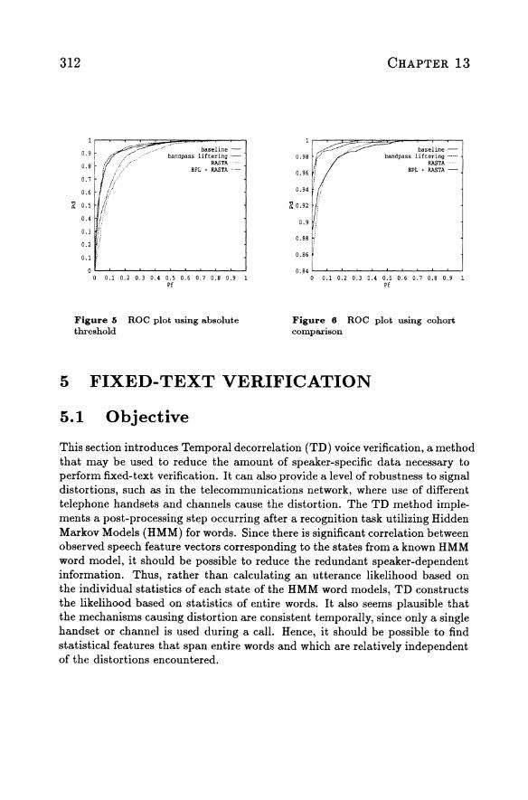
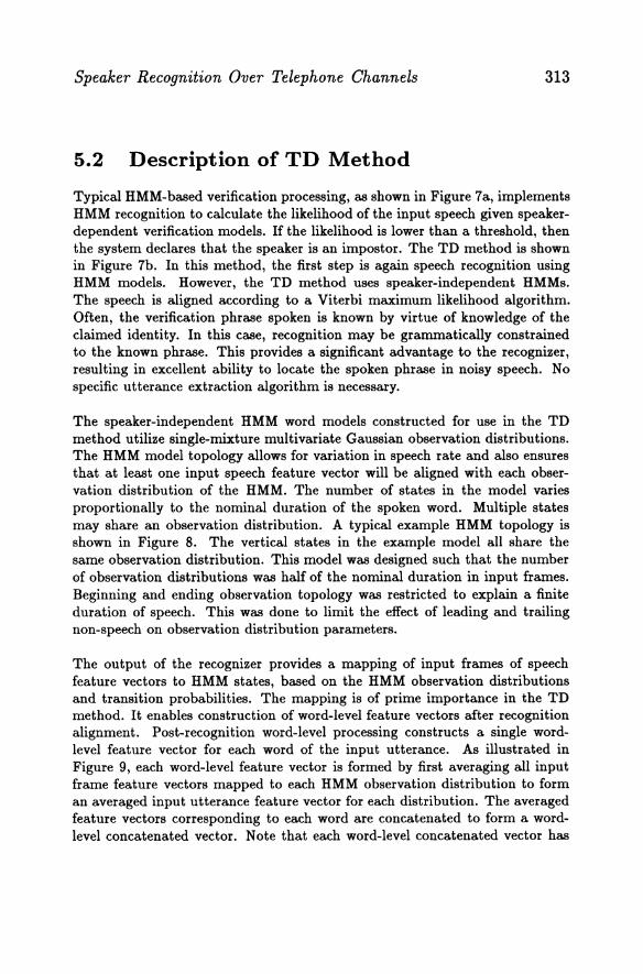
Figures 5 and 6, show that the equal error rate was reduced to less than half in all four front-end methods when using cohort comparison instead of an absolute threshold. The following table shows the equal error rates in Figures 5 and 6.

Equal error rate Front-end absolute threshold cohort comparison

Baseline 13% 5.5% BPL 12% 2.5%

RASTA 21% 6% BPL + RASTA 18% 2.5%

312

0.7

0.6

" 0.5 0.

0.4

O.l

0.2

0.1

0 0

baseline -bandpass liftering ._-.

RASTA .. BPL + RASTA ----

0.1 0.2 O.l 0.4 0.5 0.6 0.7 0.8 0.9 1 Pf

Figure (; ROC plot using absolute threshold

0.98 r;<~· I:

0.96 !

0.94

'& 0.92

0.9

0.88 i

0.86 '

CHAPTER 13

baseline -bandpass liftering ----­

RASTA . 8PL + RASTA -

o. 84 L-~-"-~--,_-,---,-~--,_-"---' o 0.1 0.2 O.l 0.4 0.5 0.6 0.7 0.8 0.9 1

Pf

Figure 6 ROC plot using cohort comparison

5 FIXED-TEXT VERIFICATION

5.1 Objective

This section introduces Temporal decor relation (TD) voice verification, a method that may be used to reduce the amount of speaker-specific data necessary to perform fixed-text verification. It can also provide a level of robustness to signal distortions, such as in the telecommunications network, where use of different telephone handsets and channels cause the distortion. The TD method imple­ments a post-processing step occurring after a recognition task utilizing Hidden Markov Models (HMM) for words. Since there is significant correlation between observed speech feature vectors corresponding to the states from a known HMM word model, it should be possible to reduce the redundant speaker-dependent information. Thus, rather than calculating an utterance likelihood based on the individual statistics of each state of the HMM word models, TD constructs the likelihood based on statistics of entire words. It also seems plausible that the mechanisms causing distortion are consistent temporally, since only a single handset or channel is used during a call. Hence, it should be possible to find statistical features that span entire words and which are relatively independent of the distortions encountered.

Speaker Recognition Over Telephone Channels 313

5.2 Description of TD Method

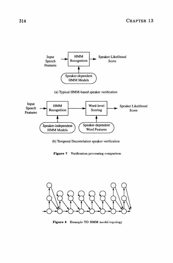
Typical HMM-based verification processing, as shown in Figure 7a, implements HMM recognition to calculate the likelihood of the input speech given speaker­dependent verification models. If the likelihood is lower than a threshold, then the system declares that the speaker is an impostor. The TO method is shown in Figure 7b. In this method, the first step is again speech recognition using HMM models. However, the TO method uses speaker-independent HMMs. The speech is aligned according to a Viterbi maximum likelihood algorithm. Often, the verification phrase spoken is known by virtue of knowledge of the claimed identity. In this case, recognition may be grammatically constrained to the known phrase. This provides a significant advantage to the recognizer, resulting in excellent ability to locate the spoken phrase in noisy speech. No specific utterance extraction algorithm is necessary.

The speaker-independent HMM word models constructed for use in the TO method utilize single-mixture multivariate Gaussian observation distributions. The HMM model topology allows for variation in speech rate and also ensures that at least one input speech feature vector will be aligned with each obser­vation distribution of the HMM. The number of states in the model varies proportionally to the nominal duration of the spoken word. Multiple states may share an observation distribution. A typical example HMM topology is shown in Figure 8. The vertical states in the example model all share the same observation distribution. This model was designed such that the number of observation distributions was half of the nominal duration in input frames. Beginning and ending observation topology was restricted to explain a finite duration of speech. This was done to limit the effect of leading and trailing non-speech on observation distribution parameters.

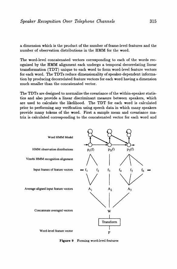
The output of the recognizer provides a mapping of input frames of speech feature vectors to HMM states, based on the HMM observation distributions and transition probabilities. The mapping is of prime importance in the TO method. It enables construction of word-level feature vectors after recognition alignment. Post-recognition word-level processing constructs a single word­level feature vector for each word of the input utterance. As illustrated in Figure 9, each word-level feature vector is formed by first averaging all input frame feature vectors mapped to each HMM observation distribution to form an averaged input utterance feature vector for each distribution. The averaged feature vectors corresponding to each word are concatenated to form a word­level concatenated vector. Note that each word-level concatenated vector has

314

Input Speech

Features

Input Speech

Features

HMM Recognition

Speaker Likelihood Score

(a) Typical HMM-based speaker verification

CHAPTER 13

HMM Recognition

Word-level Scoring

Speaker Likelihood Score

(b) Temporal Decorrelation speaker verification

Figure 'T Verification processing comparison

Figure 8 Example TD HMM model topology

Speaker Recognition Over Telephone Channels 315

a dimension which is the product of the number of frame-level features and the number of observation distributions in the HMM for the word.

The word-level concatenated vectors corresponding to each of the words rec­ognized by the HMM alignment each undergo a temporal decorrelating linear transformation (TOT) unique to each word to form word-level feature vectors for each word. The TOTs reduce dimensionality of speaker-dependent informa­tion by producing decorrelated feature vectors for each word having a dimension much smaller than the concatenated vector.

The TOTs are designed to normalize the covariance of the within-speaker statis­tics and also provide a linear discriminant measure between speakers, which are used to calculate the likelihood. The TOT for each word is calculated prior to performing any verification using speech data in which many speakers provide many tokens of the word. First a sample mean and covariance ma­trix is calculated corresponding to the concatenated vector for each word and

Word HMM Model

HMM observation distributions

Viterbi HMM recognition alignment /\ I ~ Input frames offeature vectors

Average aligned input feature vectors

Concatenate averaged vectors w

Word-level feature vector

I T~O,", I F

Figure 9 Forming word-level features

316 CHAPTER 13

speaker. Pooling the covariance matrices for each speaker results in a single pooled within-speaker covariance matrix for each word. The covariance matrices and means corresponding to the word for all speakers are then used to calculate a total covariance matrix which represents the covariance of all concatenated vectors from all speakers. Simultaneous diagonalization by eigenvector anal­ysis [21] is performed using the pooled within-speaker and total covariances. The resulting word-level features which best discriminate between speakers are retained to form the TDT for each word.

Each speaker enrolls by speaking a uniquely assigned phrase several times. The average of each word-level feature vector is calculated over all enrollment utterances, resulting in a set of speaker-dependent word-level reference vectors.

During verification, a subject wishing to be verified first provides some claim to identity. This is used to obtain the set of word-level reference feature vectors for that identity. The subject then speaks the uniquely assigned phrase, and word-level feature vectors are formed from the input speech. The input and ref­erence word-level feature vectors are compared to generate a likelihood measure, typically using a Euclidean distance. The likelihood measure for each word is weighted by the relative duration of each word to obtain a final single likelihood measure which is compared to a threshold to make the true speaker/impostor decision.

5.3 Experimental Results

The TD method has been tested using the digits zero through nine and oh as words. The TD method was tested using the Digit Verification corpus for true-speaker and impostor data. The Additional Training corpus was only used as a source for additional statistical training of the TDTs.

For all experiments the input frame-level feature vectors and HMM observa­tion distributions had a dimension of 16. Frame level features were derived from initial frame-level energy, filter-bank, and filter-bank difference data [22]. The TDTs reduced the word-level concatenated vectors for each word to a 20 element feature vector.

Enrollment was accomplished using the first call for each of the test speakers. Hence, there were three tokens of each test speaker's ten-digit phrase used for enrollment. Enrollment consisted of aligning the test speaker's input speech vectors with the speaker-independent HMM models, and calculating the aver-

Speaker Recognition Over Telephone Channels

l00~------------------------~

~ 10

J .9 i '" .1 2 - 1 - TOT closed test

2 - TOT open test 3 - HMM likelihood 3

.01 '"--------------------__ ---' .01.1 10 100

True Speaker Rejection (%)

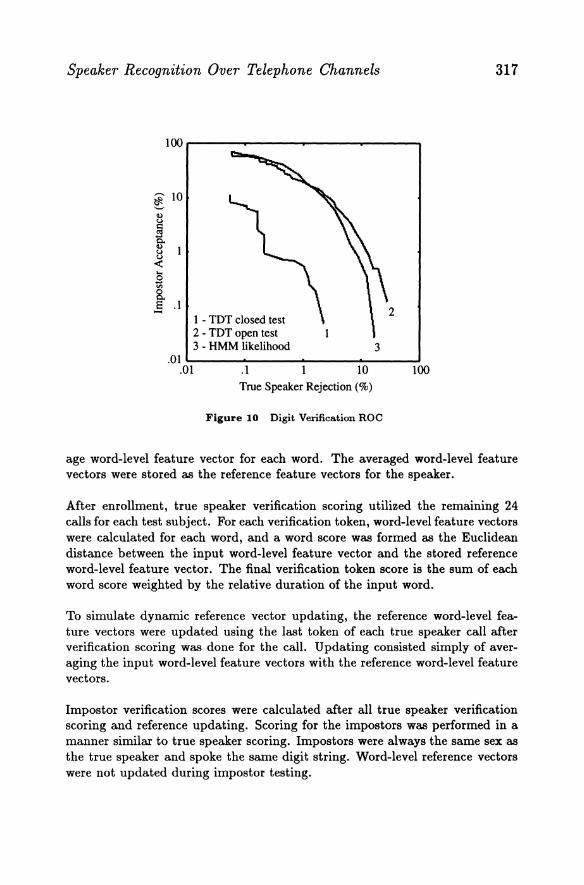
Figure 10 Digit Verification ROC

317

age word-level feature vector for each word. The averaged word-level feature vectors were stored as the reference feature vectors for the speaker.

After enrollment, true speaker verification scoring utilized the remaining 24 calls for each test subject. For each verification token, word-level feature vectors were calculated for each word, and a word score was formed as the Euclidean distance between the input word-level feature vector and the stored reference word-level feature vector. The final verification token score is the sum of each word score weighted by the relative duration of the input word.

To simulate dynamic reference vector updating, the reference word-level fea­ture vectors were updated using the last token of each true speaker call after verification scoring was done for the call. Updating consisted simply of aver­aging the input word-level feature vectors with the reference word-level feature vectors.

Impostor verification scores were calculated after all true speaker verification scoring and reference updating. Scoring for the impostors was performed in a manner similar to true speaker scoring. Impostors were always the same sex as the true speaker and spoke the same digit string. Word-level reference vectors were not updated during impostor testing.

318

l00~----------~------------~

1 - TOT closed test 2 - TDT open test 3 - HMM likelihood

2

3 .01 L-__________________ .o.-____ ...J

CHAPTER 13

.01.1 10 100 True Speaker Rejection (%)

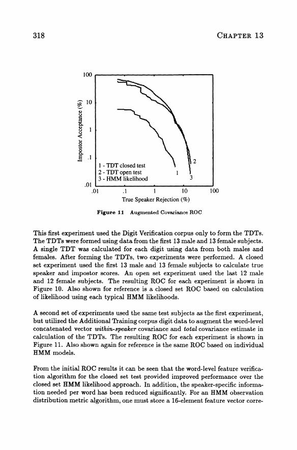
Figure 11 Augmented Covariance ROC

This first experiment used the Digit Verification corpus only to form the TOTs. The TOTs were formed using data from the first 13 male and 13 female subjects. A single TOT was calculated for each digit using data from both males and females. After forming the TOTs, two experiments were performed. A closed set experiment used the first 13 male and 13 female subjects to calculate true speaker and impostor scores. An open set experiment used the last 12 male and 12 female subjects. The resulting ROC for each experiment is shown in Figure 10. Also shown for reference is a closed set ROC based on calculation of likelihood using each typical HMM likelihoods.

A second set of experiments used the same test subjects as the first experiment, but utilized the Additional Training corpus digit data to augment the word-level concatenated vector within-speaker covariance and total covariance estimate in calculation of the TOTs. The resulting ROC for each experiment is shown in Figure 11. Also shown again for reference is the same ROC based on individual HMM models.

From the initial ROC results it can be seen that the word-level feature verifica­tion algorithm for the closed set test provided improved performance over the closed set HMM likelihood approach. In addition, the speaker-specific informa­tion needed per word has been reduced significantly. For an HMM observation distribution metric algorithm, one must store a 16-element feature vector corre-

Speaker Recognition Over Telephone Channels 319

sponding to each distribution in the HMM (typically this results in 128 values for the digit HMM structure used in these experiments). This should be com­pared with only 20 word-level features. The word-level feature performance for the open set test in Figure 10, however, did not provide improved performance over the HMM observation model approach.

Of importance in the results is the discrepancy between the closed-set and open-set results. The superior performance of the closed-set results in Figure 10 implies that the TDTs are matched to the closed-set subjects used to generate the TDTs. This has implications for speaker identification algorithms, and methods of enrollment. When data from the Additional Training corpus were used to augment word-level covariance estimates in Figure 11, as expected, closed-set performance degraded while open-set performance improved. This indicates the challenge in estimating the TDTs, which is that estimation of the large dimension of word-level covariance matrices requires large amounts of data. Presently, additional collection of digit data over long-distance telephone lines is under way that will improve covariance estimates. One can at least be assured that the best open-set performance lies somewhere between the closed-set and open-set results in Figure 11.

6 CONCLUSIONS

In this chapter we have presented methods for free-text and fixed-text speaker identification and verification over telephone channels. We have discussed chal­lenges that are faced due to the variability of the speech signal in a telephone environment. VQ free-text speaker identification has been shown to be more robust when it incorporates bandpass liftering and RASTA filtering. The con­cept of cohort comparison used in speaker identification was adapted to form a ranking algorithm which was shown to significantly improve performance in a closed-set VQ-based speaker verification test.

We introduced Temporal Decorrelation, a method of using HMMs in fixed-text speaker verification to greatly reduce the amount of speaker-dependent infor­mation that must be retained. This method also shows promise for improved verification performance over the simple HMM likelihood approach, and avoids the necessity of making an explicit speech or silence decision required by VQ methods. Comparison of closed-set testing of TD with free-text VQ cohort ranking indicates improved performance due to the advantage of fixed-text alignment, even though TD testing did not use cohort ranking.

320 CHAPTER 13

The drawback of the TD method is the large amount of training data necessary to generate decorrelating transformations for each word used in verification. Work is under way to gather additional training data over telephone channels to improve the transformations.

Even with the above improvements, the telephone channel still remains a chal­lenge. Methods of compensating for channel effects, and development of robust features and processing methods will continue to be important areas of research.

REFERENCES

[1] S. Furui, "Research on Individuality Features in Speech Waves and Auto­matic Speaker Recognition Techniques," Speech Communication, Vol. 5, 1986, pp. 183 - 197.

[2] G. Doddington, "Speaker Recognition - Identifying People by Their Voices," Proceedings of the IEEE, Vol. 73, No 11, Nov. 1985.

[3] D. O'Shaughnessy "Speaker Recognition," IEEE ASSP Magazine, Oct. 1986.

[4] A. Rosenberg "Automatic Speaker Verification: A Review," Proceedings of the IEEE, Vol. 64, No 4, Apr. 1976.

[5] B. Atal, "Automatic Recognition of Speakers from Their Voices," Proceed­ing ofIEEE, Vol. 64, No 4, Apr. 1976.

[6] M. Sambur, "Selection of Acoustic Features for Speaker Identification," IEEE Transactions on ASSP-23, No.2, Apr. 1975, pp. 176 - 182.

[7] Y.H. Kao, J. Baras, and P.K. Rajasekaran, "Robustness Study of Free-Text Speaker Identification and Verification," ICASSP 1993, pp. 379 - 382.

[8] H. Gish, "Robust Discrimination in Automatic Speaker Identification," ICASSP 1990, pp. 289 - 292.

[9] A. Acero, "Acoustical and Environmental Robustness in Automatic Speech Recognition," Ph.D. Dissertation, Carnegie Mellon University, 1990.

[10] R.C. Rose, J. Fitzmaurice, E.M. Hofstetter, and D.A. Reynolds, "Ro­bust Speaker Identification in Noisy Environments Using Noise Adaptive Speaker Models," ICASSP 1991, pp. 401- 404.

Speaker Recognition Over Telephone Channels 321

[11] J.M. Naik, L.P. Netsch, and G.R. Doddington, "Speaker Verification Over Long Distance Telephone Lines," ICASSP 1989, pp. 524 - 527.

[12] T. Matsui and S. Furui, "A Text-Independent Speaker Recognition Method Robust Against Utterance Variations," ICASSP 1991, pp. 377 - 380.

[13] F. Soong, A. Rosenberg, B.H. Juang, and L. R. Rabiner "A Vector Quanti­zation Approach to Speaker Recognition," AT&T Technical Report, 1976.

[14] T. Matsui and S. Furui, "Comparison of Text-Independent Speaker Recog­nition Methods Using VQ-Distortion and Discrete / Continuous HMM," ICASSP 1992, Vol. 2, pp. 157 - 160.

[15] L. Netsch and G. Doddington, "Speaker Verification Using Temporal Decorrelation Post Processing," ICASSP 1992, Vol. 2, pp. 181 - 184.

[16] A.L. Higgins and L.G. Bahler, "Text-Independent Speaker Verification by Discriminant Counting," ICASSP 1991, pp. 405 - 408.

[17] "Speaker Recognition Feasibility Study", Final Report, Contract No. 85F101500, January, 1987.

[18] J.J. Godfrey, E.C. Holliman, and J. McDaniel, "SWITCHBOARD: Tele­phone Speech Corpus for Research and Development," ICASSP 92, Vol. 1, pp. 517 - 520.

[19] B.H. Juang, L.R. Rabiner, and J.G. Wilpon, "On the Use of Bandpass Liftering in Speech Recognition," IEEE Transactions on ASSP-35, No.7, July, 1987.

[20] H. Hermansky, N. Morgan, A. Bayya, and P. Kohn, "RASTA-PLP Speech Analysis Technique," ICASSP 1992, Vol. 1, pp. 121 - 124.

[21] K. Fukunaga, "Introduction to Statistical Pattern Recognition," Aca­demic, 1972.

[22] G. Doddington, "Phonetically Sensitive Discriminants for Improved Speech Recognition," ICASSP 1989, Vol. 1, pp. 556 - 559.