DOCTrMFEfT OFFICE 26-327RESEARCH LABORATORY OF TECTRONICSMASSACHUSETTS INSTITUTE OF TECHNOLOGY

q,,# Cqe_'V

DIGITAL COMMUNICATIONOVER FIXED TIME-CONTINUOUS CHANNELS WITH MEMORY-

WITH SPECIAL APPLICATION TO TELEPHONE CHANNELS

J. L. HOLSINGER

RESEARCH LABORATORY OF ELECTRONICS

TECHNICAL REPORT 430

LINCOLN LABORATORY

TECHNICAL REPORT 366

OCTOBER 20, 1964

MASSACHUSETTS INSTITUTE OF TECHNOLOGYCAMBRIDGE, MASSACHUSETTS

,et-

The Research Laboratory of Electronics is an interdepartmentallaboratory in which faculty members and graduate students fromnumerous academic departments conduct research.

The research reported in this document was made possible inpart by support extended the Massachusetts Institute of Tech-nology, Research Laboratory of Electronics, by the JOINT SERV-ICES ELECTRONICS PROGRAMS (U. S. Army, U. S. Navy, andU. S. Air Force) under Contract No. DA36-039-AMC-03200 (E);additional support was received from the National Science Founda-tion (Grant GP-2495), the National Institutes of Health (GrantMH-04737-04), and the National Aeronautics and Space Adminis-tration (Grants NsG-334 and NsG-496).

The research reported in this document was also performed atLincoln Laboratory, a center for research operated by the Massa-chusetts Institute of Technology with the support of the UnitedStates Air Force under Contract AF19 (628) -500.

Reproduction in whole or in part is permitted for any purposeof the United States Government.

MASSACHUSETTS INSTITUTE OF TECHNOLOGY

RESEARCH LABORATORY OF ELECTRONICS

Technical Report 430

LINCOLN LABORATORY

Technical Report 366

October 20, 1964

DIGITAL COMMUNICATION

OVER FIXED TIME-CONTINUOUS CHANNELS WITH MEMORY--

WITH SPECIAL APPLICATION TO TELEPHONE CHANNELS

J. L. Holsinger

This report is based on a thesis submitted to the Department of Elec-trical Engineering, M. I. T., October 1964, in partial fulfillment ofthe requirements for the Degree of Doctor of Philosophy.

Abstract

The objective of this study is to determine the performance, or a bound on the per-formance, of the "best possible" method for digital communication over fixed time-continuous channels with memory, i. e., channels with intersymbol interference and/orcolored noise. The channel model assumed is a linear, time-invariant filter followed byadditive, colored Gaussian noise. A general problem formulation is introduced whichinvolves use of this channel once for T seconds to communicate one of M signals. Twoquestions are considered: (1) given a set of signals, what is the probability of error?and (2) how should these signals be selected to minimize the probability of error? It isshown that answers to these questions are possible when a suitable vector space repre-sentation is used, and the basis functions required for this representation are presented.Using this representation and the random coding technique, a bound on the probability oferror for a random ensemble of signals is determined and the structure of the ensembleof signals yielding a minimum error bound is derived. The inter-relation of coding andmodulation in this analysis is discussed and it is concluded that: (1) the optimumensemble of signals involves an impractical mddulation technique, and (2) the errorbound for the optimum ensemble of signals provides a "best possible" result againstwhich more practical modulation techniques may be compared. Subsequently, severalsuboptimurn modulation techniques are considered, and one is selected as practical fortelephone channels. A theoretical analysis indicates that this modulation system shouldachieve a data rate of about 13,000 bits/second on a data grade telephone line with an

error probability of approximately 10 5 . An experimental program substantiates thatthis potential improvement could be realized in practice.

I

TABLE OF CONTENTS

CHAPTER I- DIGITAL COMMUNICATION OVER TELEPHONE LINES 1

A. History 1

B. Current Interest 1

C. Review of Current Technology 1

D. Characteristics of Telephone Line as Channelfor Digital Communication 2

E. Mathematical Model for Digital Communication over Fixed Time-Continuous Channels with Memory 4

CHAPTER II- SIGNAL REPRESENTATION PROBLEM 7

A. Introduction 7

B. Signal Representation 7

C. Dimensionality of Finite Set of Signals 10

D. Signal Representation for Fixed Time-Continuous Channelswith Memory 12

CHAPTER III - ERROR BOUNDS AND SIGNAL DESIGN FOR DIGITALCOMMUNICATION OVER FIXED TIME-CONTINUOUSCHANNELS WITH MEMORY 37

A. Vector Dimensionality Problem 37

B. Random Coding Technique 37

C. Random Coding Bound 39

L. Bound for "Very Noisy" Channels 44

E. Improved Low-Rate Random Coding Bound 46

F. Optimum Signal Design Implications of Coding Bounds 53

G. Dimensionality of Communication Channel 54

CHAPTER IV- STUDY OF SUBOPTIMUM MODULATION TECHNIQUES 57

A. Signal Design to Eliminate Intersymbol Interference 58

B. Receiver Filter Design to Eliminate Intersymbol Interference 76

C. Substitution of Sinusoids for Eigenfunctions 82

CHAPTER V- EXPERIMENTAL PROGRAM 95

A. Simulated Channel Tests 95

B. Dial-Up Circuit Tests 98

C. Schedule 4 Data Circuit Tests 99

APPENDIX A - Proof that the Kernels of Theorems 1 to 3 Are Y2 101

APPENDIX B- Derivation of Asymptotic Form of Error Exponents 104

APPENDIX C - Derivation of Equation (63) 107

iii

CONTENTS

APPENDIX D - Derivation of Equation (70)

APPENDIX E- Proof of Even-Odd Property of NondegenerateEigenfunctions

APPENDIX F- Optimum Time-Limited Signals for Colored Noise

Acknowledgment

References

iv

109

110

111

113

114

__ _

DIGITAL COMMUNICATION

OVER FIXED TIME-CONTINUOUS CHANNELS WITH MEMORY -

WITH SPECIAL APPLICATION TO TELEPHONE CHANNELS

CHAPTER I

DIGITAL COMMUNICATION OVER TELEPHONE LINES

A. HISTORY

An interest in low-speed digital communication over telephone circuits has existed for many

years. As early as 1919, the transmission of teletype and telegraph data had been attempted

over both long-distance land lines and transoceanic cables. During these experiments it was

recognized that data rates would be severely limited by signal distortion arising from nonlinear

phase characteristics of the telephone line. This effect, although present in voice communica-

tion, had not been previously noticed due to the insensitivity of the human ear to phase distor-

tion. Recognition of this problem led to fundamental studies by Carson, ' Nyquist, 5 6 and

others. 7 From these studies came techniques, presented around 1930, for quantitatively meas-

uring phase distortion 8 and for equalizing lines with such distortion.9 This work apparently

resolved the existing problems, and little or no additional work appears to have been done un-

til the early 1950's.

B. CURRENT INTEREST

The advent of the digital computer in the early 1950's and the resulting military and com-

mercial interest in large-scale information processing systems led to a new interest in using

telephone lines for transmitting digital information. This time, however, the high operating

speeds of these systems, coupled with the possibility of a widespread use of telephone lines,

made it desirable to attempt a more efficient utilization of the telephone channel. Starting about

1954, people at both Lincoln Laboratory1 0 ' l and Bell Telephone Laboratories12 - 14 began in-

vestigating this problem. These and other studies were continued by a moderate but ever in-

creasing number of people during the late 1950's. 1 5 - 2 1 By 1960, numerous systems for obtain-

ing high data rates (over 500 bits/second) had been proposed, built, and tested.2 2 - 3 0 These

systems were, however, still quite poor in comparison to what many people felt to be possible.

Because of this, and due also to a growing interest in the application of coding techniques to

this problem, work has continued at a rapidly increasing pace up to the present. Today

it is necessary only to read magazines such as Fortune, Business Week, or U. S. News and

World Report to observe the widespread interest in this use of the telephone network. 4 4 4 7

C. REVIEW OF CURRENT TECHNOLOGY

The following paragraphs discuss some of the current data transmission systems, or

modems (modulator-demodulator), and indicate the basic techniques used along with the resulting

performance. Such state-of-the-art information is useful in evaluating the theoretical results

obtained in the subsequent analysis.

_- _s --_

Two numbers often used in comparing digital communication systems are rate R in bits

per second and the probability of error Pe. However, the peculiar properties of telephone

channels (Sec. I-D) cause the situation to be quite different here. In fact, most present modems

operating on a telephone line whose phase distortion is within "specified limits" have a P of 10 4-6 e

to 10 that is essentially independent of rate as long as the rate is below some maximum value.

As a result, numbers useful for comparison purposes are the maximum rate and the "specified

limit" on phase distortion; the latter number is usually defined as the maximum allowable dif-

ferential delayt over the telephone line passband.

Probably the best-known current modems are those used by the Bell Telephone System in

the Data-Phone service. 3 3 At present, at least two basic systems cover the range from 500 to

approximately 2400 bits/second. The simplest of these modems is an FSK system operating at

600 or 1200 bits/second. Alexander, Gryb, and Nast 3 3 have found that the 600-bits/second

system will operate without phase compensation over essentially any telephone circuit in the

country and that the 1200-bits/second system will operate over most circuits with a "universal"

phase compensator. A second system used by Bell for rates of about 2400 bits/second is a

single frequency four-phase differentially modulated system. 4 8 At present, little additional

information is available concerning the sensitivity of this system to phase distortion.

Another system operating at rates of 2400 to 4800 bits/second has been developed by Rixon

Electronics, Inc. ,29 This modem uses binary AM with vestigial side-band transmission and

requires telephone lines having maximum differential delays of 200 to 400 sec.

A third system, the Collins Radio Company Kineplex, 2 7 4 9 has been designed to obtain data

rates of 4000 to 5000 bits/second. This modem was one of the first to use signal design tech-

niques in an attempt to overcome some of the special problems encountered on the telephone

channel. Basically, this system uses four-phase differential modulation of several sinusoidal

carriers spaced in frequency throughout the telephone line passband. The differential delay

requirements for this system are essentially the same as for the Rixon system at high rate,

i.e., about 200 sec.

Probably the most sophisticated of the modems constructed to date was used at Lincoln

Laboratory in a recently reported experiment. 43 In this system, the transmitted signal was

"matched" to the telephone line so that the effect of phase distortion was essentially eliminated.t

Use of this modem with the SECO50 machine (a sequential coder-decoder) and a feedback channel

allowed virtually error-free transmission at an average rate of 7500 bits/second.

D. CHARACTERISTICS OF TELEPHONE LINE AS CHANNELFOR DIGITAL COMMUNICATION

Since telephone lines have been designed primarily for voice communication, and since the

properties required for voice transmission differ greatly from those required for digital trans-

mission, numerous studies have been made to evaluate the properties that are most significant

for this application (see Refs. 10, 12, 14, 17, 31, 33). One of the first properties to be recognized

was the wide variation of detailed characteristics of different lines. However, later studies

t Absolute time delay is defined to be the derivative, with respect to radian frequency, of the telephone linephase characteristic. Differential delay is defined in terms of this by subtracting out any constant delay. Thedifferential delay for a "typical" telephone line might be 4 to 6 msec at the band edges.

I This same approach appears to have been developed independently at IBM.4 2

2

have shown 3 3 that only a few phenomena are responsible for the characteristics that affect digital

communication most significantly. In an order more or less indicative of their relative impor-

tance, these are as follows.

Intersymbol Interferencet:- Intersymbol interference is a term commonly applied to an

undesired overlap (in time) of received signals that were transmitted as separate pulses. This

effect is caused by both the finite bandwidth and the nonlinear phase characteristic of the tele-

phone line, and leads to significant errors even in the absence of noise or to a significant reduc-

tion in the signaling rate.1 It is possible to show, however, that the nonlinear phase character-

istic is the primary source of intersymbol interference.

The severity of the intersymbol interference problem can be appreciated from the fact that

the maximum rate of current modems is essentially determined by two factors: (1) the sensi-

tivity of the particular signaling scheme to intersymbol interference, and (2) the "specified

limit" on phase distortion; the latter being in some sense a specification of allowable inter-

symbol interference. In none of these systems does noise play a significant role in determining

rate as it does, for example, in the classical additive, white Gaussian noise channel.5 1 Thus,

current modems trade rate for sensitivity to phase distortion - a higher rate requiring a lower

"specified limit" on phase distortion and vice versa.

Impulse and Low-Level Noise:- Experience has shown that the noise at the output of a tele-

phone line appears to be the sum of two basic types.3133 One type of noise, low-level noise, is

typically 20 to 50 db below normal signal levels and has the appearance of Gaussian noise super-

imposed on harmonics of 60 cps. The level and character of this noise is such that it has neg-

ligible effect on the performance of current modems. The second type of noise, impulse noise,

differs from low-level noise in several basic attributes. 5 2 First, its appearance when viewed

on an oscilloscope is that of rather widely separated (on the order of seconds, minutes, or

even days) bursts of relatively long (on the order of 5 to 50 msec) transient pulses. Second, the

level of impulse noise may be as much as 10 db above normal signal levels. Third, impulse

noise appears difficult to characterize in a statistical manner suitable for deriving optimum

detectors. Because of these characteristics, present modems make little or no attempt to

combat impulse noise; furthermore, impulse noise is the major source of errors in these sys-

tems. In fact, most systems operating at a rate such that intersymbol interference is a neg-

ligible factor in determining probability of error will be found to have an error rate almost

entirely dependent upon impulse noise - typical error rates being 1 in 10 to 1 in 10 (Ref. 33).

Phase Crawl:- Phase crawl is a term applying to the situation in which the received signal

spectrum is displaced in frequency from the transmitted spectrum. Typical displacements are

from 0 to 10 cps and arise from the use of nonsynchronous oscillators in frequency translations

performed by the telephone company. Current systems overcome this effect by various modu-

lation techniques such as AM vestigial sideband, differentially modulated FM, and carrier re-

covery with re-insertion.

Dropout:- The phenomena called dropout occurs when for some reason the telephone line ap-

pears as a noisy open circuit. Dropouts are usually thought to last for only a small fraction of a

I Implicit in the following discussion of intersymbol interference is the assumption that the telephone line is alinear device. Although this may not be strictly true, it appears to be a valid approximation in most situations.

$ Alternately, and equivalently, intersymbol interference can be viewed in the time domain as arising from thelong impulse response of the line (typically 10 to 15 msec duration).

3

second, although an accidental opening of the line can clearly lead to a much longer dropout.

Little can be done to combat this effect except for the use of coding techniques.

Crosstalk:- Crosstalk arises from electromagnetic coupling between two or more lines in

the same cable. Currently, this is a secondary problem relative to intersymbol interference

and impulse noise.

The previous discussion has indicated the characteristics of telephone lines that affect digital

communication most significantly. It must be emphasized, however, that present modems are

limited in performance almost entirely by intersymbol interference and impulse noise. The

maximum rate is determined primarily by intersymbol interference and the probability of error

is determined primarily by impulse noise. Thus, an improved signaling scheme that consider-

ably reduces intersymbol interference should allow a significant increase in data rate with a

negligible increase in probability of error. Some justification for believing that this improve-

ment is possible in practice is given by the experiment at Lincoln Laboratory.4 3 In this experi-

ment, a combination of coding and a signal design that reduced intersymbol interference allowed

performance significantly greater than any achieved previously. Even so, the procedure for

combating intersymbol interference was ad hoc. Thus, the primary objective of this report is

to obtain a fundamental theoretical understanding of optimum signaling techniques for channels

whose characteristics are similar to those of the telephone line.

E. MATHEMATICAL MODEL FOR DIGITAL COMMUNICATION OVER FIXED TIME-CONTINUOUS CHANNELS WITH MEMORY

1. Introduction

Basic to a meaningful theoretical study of a real life problem is a model that includes the

important features of the real problem and yet is mathematically tractable. This section pre-

sents a relatively simple, but heretofore incompletely analyzed, model that forms the basis for

the subsequent theoretical work. There are two fundamental reasons for this choice of model:

(a) It represents a generalization of the classical white, Gaussiannoise channel considered by Fano, 5 1 Shannon, 5 3 and others. Thus,any analysis of this channel represents a generalization of pre-vious work and is of interest independently of any telephone lineconsiderations.

(b) As indicated previously, the performance of present telephoneline communication systems is limited in rate by intersymbolinterference and in probability of error by impulse noise; thelow-level "Gaussian" noise has virtually no effect on systemperformance. However, the frequent occurrence of long inter-vals without significant impulse noise activity makes it desirableto study a channel which involves only intersymbol interference(it is time dispersive) and Gaussian noise. In this manner, itwill be possible to learn how to reduce intersymbol interferenceand thus increase rate to the point where errors caused by low-level noise are approximately equal in number to errors causedby impulse noise.

2. Some Considerations in Choosing a Model

One of the fundamental aims of the present theoretical work is to determine the performance,

or a bound on the performance, of the "best possible" method for digital communication over

fixed time-continuous channels with memory, i.e., channels with intersymbol interference

4

� ��_ _�

and/or colored noise. In keeping with this goal, it is desirable to include in the model only

those features that are fundamental to the problem when all practical considerations are removed.

For example, practical constraints often require that digital communication be accomplished by

the serial transmission of short, relatively simple pulses having only two possible amplitudes.

The theoretical analysis will show, however, that for many channels this leads to an extremely

inefficient use of the available channel capacity. In other situations, when communication over

a narrow-band, bandpass channel is desired, it is often convenient to derive the transmitted

signal by using a baseband signal to amplitude, phase or frequency modulate a sinusoidal carrier.

However, on a wide-band, bandpass channel such as the telephone line it is not a priori clear

that this approach is still useful or appropriate although it is certainly still possible. Finally,

it should be recognized that the interest in a model for digitalt communication implies that de-

tection and decision theory concepts are appropriate as opposed to least-mean-square error

filtering concepts that find application in analog communication.

3. Model

An appropriate model for digital communication over fixed time-dispersive channels can

be specified in the following manner. An obvious but fundamental fact is that in any real situa-

tion it is necessary to transmit information for only a finite time, say T seconds. This, cou-

pled with the fact that a model for digital communication is desired, implies that one of only a

finite number, say M, of possible messages is to be transmitted.$ For the physical situation

being considered, it is useful to think of transmitting this message by establishing a one-to-one

correspondence between a set of M signals of T seconds duration and transmitting the signal

that corresponds to the desired message. Furthermore, in any physical situation, there is only

a finite amount of energy, say ST, available with which to transmit the signal. (Implicit here

is the interpretation of S as average signal power.) This fact leads to the assumption of some

form of an energy constraint on the set of signals - a particularly convenient constraint being

that the statistical average of the signal energies is no greater than ST. Thus, if the signals

are denoted by si(t) and each signal is transmitted with probability Pi, the constraint is

M .

Pi si 2 (t) dt ST (1)

i=l

Next, the time-dispersive nature of the channel must be included in the model. A model

for this effect is simply a linear time-invariant filter. The only assumption required on this

filter is that its impulse response have finite energy, i.e., that

h2 (t) dt < - (2)

t The word "digital" is used here and throughout this work to mean that there are only a finite number of possiblemessages in a finite time interval. It should not be construed to mean "the transmission of binary symbols" oranything equally restrictive.

tAt this point, no practical restrictions will be placed on T or M. So, for example, perfectly allowable valuesfor T and M might be T = 3 X 107 seconds 1 year and M = 111. This is done to allow for a very general for-mulation of the problem. Later analysis will consider more practical situations.

5

_ -__

It is convenient, however, to assume, as is done through this work, that the filter is normalized

so that max IH(f) 1 = 1, wheref

H(f) h(t) e - jWt dt

Furthermore, to make the entire problem nontrivial, some noise must be considered. Since the

assumption of Gaussian noise leads to mathematically tractable results and since a portion of the

noise on telephone lines appears to be "approximately" Gaussian, this form for the noise is as-

sumed in the model. Moreover, since actual noise appears to be additive, that is also assumed.

For purposes of generality, however, the noise will be assumed to have an arbitrary spectral

density N(f).

Finally, to enable the receiver to determine the transmitted message it is necessary to

observe the received signal (the filtered transmitted signal corrupted by the additive noise) over

an interval of, say T1 seconds, and to make a decision based upon this observationt

In summary, the model to be analyzed is the following: given a set of M signals of T seconds

duration satisfying the energy constraint of Eq. (1), a message is to be transmitted by selecting

one of the signals and transmitting it through the linear filter h(t). The filter output is assumed

to be corrupted by (possibly colored) Gaussian noise and the receiver is to decide which message

was transmitted by observing the corrupted signal for T1 seconds.

Given the above model, a meaningful performance criterion is probability of error. On the

basis of this criterion, three fundamental questions can be posed.

Given a set of signals si(t)}, what form of decision device shouldbe used?

What is the resulting probability of error?

How should a set of signals be selected to minimize the probabilityof error?

The answer to the first question involves well-known techniques and will be discussed only

briefly in Chapter III. The determination of the answers to the remaining two questions is the

primary concern of the theoretical portion of this report.

In conclusion, it must be emphasized that the problem formulated in this section is quite

general. Thus, it allows for the possibility that optimum signals may be of the form of those

used in current modems. The formulation has not, however, included any practical constraints

on signaling schemes and thus does not preclude the possibility that an alternate and superior

technique may be found.

t At this point, T1 is completely arbitrary. Later it will prove convenient to assume T1 T which is the situationof most practical interest.

6

CHAPTER II

SIGNAL REPRESENTATION PROBLEM

A. INTRODUCTION

The previous section presented a model for digital communication over fixed time-dispersive

channels and posed three fundamental questions concerning this model However, an attempt

to obtain detailed answers to these questions involves considerable difficulty. The source of this

difficulty is that the energy constraint is applied to signals at the filter input, whereas the prob-

ability of error is determined by the structure of these signals at the filter output. Fortunately,

the choice of a signal representation that is "matched" to both the model and the desired analysis

allows the presence of the filter to be handled in a straightforward manner. The following sec-

tions present a brief discussion of the general signal representation problem, slanted, of course,

toward the present analysis, and provide the necessary background for subsequent work.

B. SIGNAL REPRESENTATION

At the outset, it should be mentioned that many of the concepts, techniques, and terminology

of this section are well known to mathematicians under the title of "Linear Algebra."5 5

As pointed out by Siebert, the fundamental goal in choosing a signal representation for a

given problem is the simplification of the resulting analysis. Thus, for a digital communication

problem, the signal representation is chosen primarily to simplify the evaluation of probability

of error. One representation which has been found to be extremely useful in such problems

(due largely to the widespread assumption of Gaussian noise) pictures signals as points in an

n-dimensional Euclidean vector space.

1. Vector Space Concept

In a digital communication problem it is necessary to represent a finite number of signals

M. One way to accomplish this is to write each signal as a linear combination of a (possibly

infinite) set of orthonormal "basis" functions {(pi(t)}, i.e.,

n

sj(t)= siji(t) (3)i=l

where

Sj = ,5 i(t) sj(t) dt

When this is done, it is found in many cases that the resulting probability of error analysis

depends only on the numbers sij and is independent of the basis functions {oi(t)}. In such cases,

a vector or n-tuple s.j can be defined as

-j j'(S1j' Sj ' S kj' ' Snj)

which, in so far as the analysis is concerned, represents the time function sj(t). Thus, it is

possible to view s. as a straightforward generalization of a three-dimensional vector and sj(t)

as a vector in an n-dimensional vector space. The utility of this viewpoint is clear from its

7

�___�I_ _ __

widespread use in the literature. Two basic reasons for this usefulness, at least in problems

with Gaussian noise, are clear from the following relations which are readily derived from

Eq. (3). The energy of a signal sj(t) is given by

n

S (t ) dt = s.j - J

i=l1

and the cross correlation between two signals si(t) and sj(t) is given by

n

sj(t) sk(t) dt = sijsik sj sk

i=l

where ( ) · ( ) denotes the standard inner product. 5 5

2. Choice of Basis Functions

So far, the discussion of the vector space representation has been concerned with basic re-

sults from the theory of orthonormal expansions. However, an attempt to answer a related

question - how are the i(t) to be chosen - leads to results that are far less well defined and less

well known. Fundamentally, this difference arises because the choice of the (qi(t) depends heavily

upon the type of analysis to be performed, i.e., the qpi(t) should be chosen to "simplify the anal-

ysis as much as possible." Since such a criterion clearly leads to no specific rule for deter-

mining the o i(t), it is possible only to indicate situations in which distinctly different basis func-

tions might be appropriate.

Band-Limited Signals:- A set of basis functions used widely for representing band-

limited signals is the set of o i(t) defined by

((t) = sin 27rW [t - (i/2W)] (4)1 2irW [t - (i/2W)l

where W is the signal bandwidth. The popularity of this representation, the so-called sampling

representation, lies almost entirely in the simple form for the coefficient s... This is readily

shown to be

Sii = S_ yi(t) sj(t) dt i sj(i/2W) . (5)

It should be recalled, however, that no physical signal can be precisely band-limited. 5 8 Thus,

any attempt to represent a physical signal by this set of basis functions must give only an ap-

proximate representation. However, it is possible to make the approximation arbitrarily accu-

rate by choosing W sufficiently large.

Time-Limited Signals:- Time-limited signals are often represented by any one of

several forms of a Fourier series. These representations are well known to engineers and any

discussion here would be superfluous. It is worth noting that this representation, in contrast

to the sampling representation, is exact for any signal of engineering interest.

Arbitrary Set of M Signals:- The previously described representations share the

property that, in general, an infinite number of basis functions are required to represent a

finite number of signals. However, in problems involving only a finite number of signals, it

8

is sometimes convenient to choose a different set of basis functions so that no more than M basis

functions are required to represent M signals. A proof that such a set exists, along with the

procedure for finding the functions, has been presented by Arthurs and Dym 5 9 This result, al-

though well known to mathematicians, appears to have just recently been recognized by electrical

engineers.

Signals Corrupted by Additive Colored Gaussian Noise:- In problems involving signals

of T seconds duration imbedded in colored Gaussian noise, it is often desirable to represent both

signals and noise by a set of basis functions such that the noise coefficients are statistically

independent random variables. If the noise autocorrelation functiont is R(T), it is well known

from the Karhunen-Loeve theorem5 4 '6 0 that the qoi(t) satisfying the integral equation

T

Xi i(T) = (i(T') R(T - T') dT 0 T ,< T

form such a set of basis functions.

Filtered Signals:- Consider the following somewhat artificial situation closely related

to the results of Sec. II-D. A set of M finite energy signals defined on the interval [0, T] is

given. Also given is a nonrealizable linear filter whose impulse response satisfies h(t) = h(-t).

It is desired to represent both the given signals and the signals that are obtained when these are

passed through the filter by orthonormal expansions defined on the interval [0, T]. In general,

arbitrary and different sets of Poi(t) can be chosen for both representations. Then the relation

between the input signal vector s and the output signal vector, say rj, is determined as follows:

Let rj(t) be the filter output when sj(t) is the filter input. Then

rj(t) (Tj( ) h(t - T) d sij !Ti(T) h(t - T) dTi0

where {cai(t) } are the basis functions for the input signals. Thus, if {Yi(t)} are the basis functions

for the output signals, it follows that

rk A rj(t) Yk(t) dt sij S Yk (t) h(t- T) (T) ddt

or, in vector notation,

rj [HI s (6)

where the k, it h element in [HI is

T T_ j_ 'Yk(t) h(t - ) cai(T) dTdt

and, in general, r and s are infinite dimensional column vectors and [HI is an infinite dimen-

sional matrix.

t For the statement made here to be strictly true, it is sufficient that R('r) be the autocorrelation function offiltered white noise 6 1

9

�--_I�--� _IIL--_l__�----·---^ --

If, however, a common set of basis functions is used for both input and output signals and

if these 'oi(t) are taken to be the solutions of the integral equation t

T

ifi( ) (Pi(T) h(t - T) dT O t T

then the relation of Eq. (6) will still be true but now [H] will be a diagonal matrix with the eigen-

values X. along the main diagonal. This result, which is related to the spectral decomposition

of linear self-adjoint operators, 2,3 has two important features. First, and most obvious, the

diagonalization of the matrix [H] leads to a much simplified calculation of r given sj. Equally

important, however, this form for [H] has entries depending only upon the filter impulse re-

sponse h(t). Although not a priori obvious, these two features are precisely those required of

a signal representation to allow evaluation of probability of error for digital transmission over

time-dispersive channels.

C. DIMENSIONALITY OF FINITE SET OF SIGNALS

This section concludes the general discussion of the signal representation problem by pre-

senting a definition of the dimensionality of a finite set of signals that is of independent interest

and is, in addition, of considerable use in defining the dimensionality of a communication channel.

An approximation often used by electrical engineers is given by the statement that a signal

which is "approximately" time-limited to T seconds and "approximately" band-limited to W cps

has 2TW "degrees of freedom"; i.e., that such a signal has a "dimensionality" of 2TW. This

approximation is usually justified by a conceptually simple but mathematically unappealing argu-

ment based upon either the sampling representation or the Fourier series representation pre-

viously discussed. However, fundamental criticisms of this statement make it desirable to

adopt a different and mathematically precise definition of "dimensionality" that overcomes these

criticisms and yet retains the intuitive appeal of the statement. Specifically, these criticisms

are:

(1) If a (strictly) band-limited nonzero signal is assumed, it is known 5 8 thatthis signal must be nonzero over any time interval of nonzero length.Thus, any definition of the "duration" T of such a signal must be arbi-trary, implying an arbitrary "dimensionality," or equally unappealing,the signal must be considered to be of infinite duration and therefore ofinfinite "dimensionality." Conversely, if a time-limited signal is as-sumed, it is known 5 8 that its energy spectrum exists for all frequencies.Thus, any attempt to define "bandwidth" for such a signal leads to sim-ilar problems. Clearly, the situation in which a signal is neither band-limited nor time-limited, e.g., s(t) = exp [- It|] where -o < t < , leadsto even more difficulties.1

(2) The fundamental importance of the concept of the "dimensionality" of asignal is that it indicates, hopefully, how many real numbers must begiven to specify the signal. Thus, when signals are represented as pointsin n-dimensional space, it is often useful to define the dimensionality ofa signal to be the dimensionality of the corresponding vector space. This

tAgain, there are mathematical restrictions on h(t) before the following statements are strictly true. Theseconditions6 4, 6 5 are concerned with the existence and completeness of the qi(t) and are of secondary interest atthis point.

f It should be mentioned that identical problems are encountered when an attempt is made to define the "dimen-sionality" of a channel in a similar manner. This problem will be discussed in detail in Chapter III.

10

definition, however, may lead to results quite different from those ob-tained using the concept of "duration" and "bandwidth." For example,consider an arbitrary finite energy signal s(t). Then by choosing foran orthonormal basis the single function

qW~) ~ s(t)

[i s2 (t) dtj

it follows that

s(t) = so l(t)

where, as usual,

S1 = s(t) (t) dt_oo

Thus, this definition of the dimensionality of s(t) indicates that it is onlyone dimensional in contrast to the arbitrary (or infinite) dimensionalityfound previously. Clearly, such diversity of results leaves something tobe desired.

Although this discussion may seem somewhat confusing and puzzling, the reason for the

widely different results is readily explained. Fundamentally, the time-bandwidth definition of

signal dimensionality is an attempt to define the "useful" dimensionality of the vector space ob-

tained when the basis functions are restricted to be either the band-limited sin x/x functions or

the time-limited sine and cosine functions. In contrast, the second definition of dimensionality

allowed an arbitrary set of basis functions and in doing so allowed the cP i(t) to be chosen to mini-

mize the dimensionality of the resulting vector space.

In view of the above discussions, and because it will prove useful later, the following defi-

nition for the dimensionality of a set of signals will be adopted:t

Let S be a set of M finite energy signals and let each signal in this set berepresented by a linear combination of a set of orthonormal functions, i.e.,

N

sj(t) = L Sijqi(t) for all sj(t) S

i=t

Then the dimensionality d of this set of signals is defined to be the minimumof N over all possible basis functions, i.e.,

d min N

{0 i(t)}

The proof that such a number d exists, that d M, and the procedure for finding the {( i(t)}

have been presented elsewhere and will not be considered here. It should be noted, however,

that the definition given is unambiguous and, as indicated, is quite useful in the later work. It

is also satisfying to note that if S is a set of band-limited signals having the property that

for all i < or i > ZTWs.(i/zW) o

for all sj(t) S

tThis definition is just the translation into engineering terminology of a standard definition of linear algebra. 55 ' 6 6

11

1- I I

then the above definition of dimensionality leads to d = 2TW. A similar result is also obtained

for a set of time-limited functions whose frequency samples all vanish except for a set of 2TW

values.

D. SIGNAL REPRESENTATION FOR FIXED TIME-CONTINUOUS CHANNELSWITH MEMORY

In Sec. I-E, it was demonstrated that a useful model for digital communication over fixed

time-continuous channels with memory considers the transmission of signals of T-seconds dura-

tion through the channel of Fig. 1 and the observation of the received signal y(t) for T1 seconds.

Given this model, the problem is to determine the probability of error for an optimum detector

and a particular set of signals and then to minimize the probability of error over the available

sets of signals. Under the assumption that the vector space representation is appropriate for

this situation, there remains the problem of selecting the basis functions for both the transmitted

signals x(t) and the received signals y(t).

13-64-30941

x(t)

n(t)

manx

y(t)

Fig. 1. Time-continuous channel with memory.

f n(t)

[I H(f) 12/N(f ] f

If x, n, and y are the (column) vector representations of the transmitted signal (assumed

to be defined on O, T), additive noise, and received signal (over the observation interval of T

seconds), respectively, an arbitrary choice of basis functions will lead to the vector equation

y = [H] x + n (7)

in which all vectors are, in general, infinite dimensional, n may have correlated components,

and [H] will be an infinite dimensional matrix related to the filter impulse response and the sets

of basis functions selected.t If, instead, both sets of basis functions are selected in the manner

presented here and elsewhere, it will be found (1) that [H] is a diagonal matrix whose entries are

the square root of the eigenvalues of a related integral equation, and (2) that the components of

n are statistically independent and identically distributed Gaussian random variables. Because

of these two properties it is possible to obtain a meaningful and relatively simple bound on prob-

ability of error for the channel considered in this work.

In the following discussion it would be possible, at least in principle, to present a single

procedure for obtaining the desired basis functions which would be valid for any filter impulse

response, any noise spectral density, and any observation interval, finite or infinite. This

approach, however, leads to a number of mathematically involved limiting arguments when

white noise and/or an infinite observation interval is of interest. Because of these difficulties

the following situations are considered separately and in the order indicated.

tit is, of course, possible to obtain statistically independent noise components by using for the receiver signalspace basis functions the orthonormal functions used in the Karhunen-Loeve expansion of the noise 5 4 ,6 0 How-ever, this will not, in general, diagonalize [H].

12

�__ __I__ _� __I �_ __

Arbitrary filter, white noise, arbitrary observation interval (arbitrary T1);

Arbitrary filter, colored noise, infinite observation interval (T1 = );

Arbitrary filter, colored noise, finite observation interval (T1 < o).

Due to their mathematical nature, the main results of this section are presented in the form

of several theorems. First, however, some assumptions and simplifying notation will be

introduced.

Assumptions.

(1) The time functions h(t), x(t), y(t), and n(t) are in all cases real.

(2) The input signal x(t) may be nonzero only on the interval [0, T] and hasfinite energy; that is, x(t) E 2(0, T) and thus

T j x2(t)dt :x(t) dt x(t) dt <

~.i0it i df~~_oo

(3) The filter impulse response h(t) is physically realizable and stable. 5 6

Thus, h(t) = 0 for t < 0 and

5 j h(t)I dt <_oo

(4) The time scale for y(t) is shifted to remove any pure delay in h(t).

(5) The observation interval for y(t) is the interval [0, T1 ], unless otherwiseindicated.

Note: Assumptions 3, 4, and 5 have been made primarily to simplify the proof that the p (t)

are complete. Clearly, these assumptions cause no loss of generality with respect to "real

world" communication problems. Furthermore, completeness proofs, although considerably

more tedious, are possible only under the assumption that

' h2 (t) dt < o_oo

Notation.

The standard inner product on the interval [0, T] is written (f, g); that is,

T(f, g) 4x f(t) g(t) dt

The linear integral operation on f(t, s) by k(t, T) is written kf(t, s); that is,

kf(t, s) A k(t, T) f(T, s) dT

The generalized inner product on the interval [0, T1] is written (f, kg) Tthat is, 1

(f, kg)T __i f(t) kg(t) dt (t) f k(t, ) g(T) d dt(f. kg 1 O:T1 ,,,,Soo

With these preliminaries the pertinent theorems can now be stated. The following results are

closely related to the spectral decomposition of linear self-adjoint operators on a Hilbert

13

~~_1^~ 1~ _ _ II III·II~- - L-. I I__~~~_._--- ---------- - -L _

space.62,63,66 It should be mentioned that all the following results can be applied directly to

time-discrete channels by simply replacing integral operators with matrix operators.

1. Basis Functions for White Noise and an Arbitrary Observation Interval

Theorem 1.

Let N(f) = 1, define a symmetric function K(t, s) =

sponse by

K(t, s) {oT h(T - t) h(T - S) dT

K(s, t) in terms of the filter impulse re-

0 t, s _ T

elsewhere

and define a set of eigenfunctions and eigenvalues by

Xi i(t) = K i(t)11 1i = 1,2,... . (8)

[Here and throughout the remainder of this work, it is assumed that i(t) = 0 for t < 0 and

t > T, i = 1, 2, .... Then the vector representation of an arbitrary x(t) E 2(0, T) is x, where

Xi = (x, Si) and the vector representation of the correspondingt y(t) on the interval [0, T 1]

(T1 > T)t is given by Eq. (7) in which the components of n are statistically independent and iden-

tically distributed Gaussian random variables with zero-mean and unit variance and

[H]

X1

I,2 0

Ff n

0

The basis functions for y(t) are {Oi(t)}, where

1 h(tp (t)

ei(t)= Aii i

TO

t Telsewhere

elsewhere

and the it h component of y is

Yi = ( y ' i)T

64,65Note: To be consistent with the literature, ' it is necessary to denote as eigenfunctions

only those solutions of Eq. (8) having Xi > 0. This restriction is required since mathematicians

normally place the eigenvalue on the right-hand side of Eq. (8) and do not consider eigenfunctions

with infinite eigenvalue.

t The representation for y(t) neglects a noise "remainder term" which is irrelevant in the present work. See thediscussion following the proof of Lemma 3 for a detailed consideration of this point.

tAIl the following statements will be true if T1 < T except that the i(t)} will not be complete in 2(0,T).

14

Proof.

The proof of this theorem consists of a series of Lemmas. The first Lemma demonstrates

that eigenfunctions of Eq. (8) form a basis for z2(0, T), i.e., that they are complete.

Lemma l(a).

If T > T, the set of functions {i(t)} defined by Eq. (8) form an orthonormal basis for f?2 (0, T),

that is, for every x(t) E 2 (0, T)

x(t) = L xii(t) 0 t < T

i=l

where x = (x, i) and mean-square convergence is obtained.

Proof.

Since the kernel of Eq. (8) is 2 (see Appendix A) and symmetric, it is well known 6 4 that at

least one eigenfunction of Eq. (8) is nonzero, that all nonzero and nondegenerate eigenfunctions

are orthogonal (and therefore may be assumed orthonormal) and that degenerate eigenfunctions

are linearly independent and of finite multiplicity and may be orthonormalized. Furthermore,

it is known 6 1 ' 6 5 that the {(Pi(t)} are complete in 2(0, T) if and only if the condition

(f, Kf)T 0 f(t) E 2 (0,T)1

implies f(t) = O almost everywhere on [0, T]. But

(f Kf)T 1 s [ f(T) h(t - T) d dt

Thus, to prove completeness, it suffices to prove that if

T

f f(r) h(t - ) d = 0 0 t T1 with T1 >_T

then f(t) = 0 almost everywhere on [O, T]. Let

u(t) =T f(T) h(t - ) dt

and assume that

O tt< Tu(t) =

z(t-T 1) t > T1

where z(t) is zero for t < 0 and is arbitrary elsewhere, except that it must be the result of

passing some 2(0, T) signal through h(t). Then

0est -sT 1

U(s) u(t) e - s t dt = e Z(s) = F(s) H(s) Re[s] > 0 (9)

Now, for Re[s] > 0,

15

-_1��--11� -���·---- I-l�--·IIIX -·___1··1·1-~- --

[Z(s) I=0o

So

z(t) e dt ' Iz(t)I exp{-Re[s] t dt-· vo·~ · · · ~~)

z(t)[ dt = 5T0 0

f(r) h(t - r) d dt

_< I f(T) h(t - T) 0 0

However, from the Schwarz inequality,

I f(T) dT [<0 L o

If(T) dT I h(t) dt_00

and, from assumption 3,

\ h(t) l dt < oJoo

Thus,

IZ(s) < [T f2 (T) d]

Since f(t) E z2(0, T), this result combined with ]

such that

IF(s) H(s) < A exp{I-Re[s] T1}

From a Lemma of Titchmarsh it follows

a + = T1, such that

IF(s) | < AI exp{-Re[s] a}

JH(s) I < AZ exp {-Re[s] 1f}

where A1A2 = A. Finally, since

f(t) = 27rj ~_' j-

|I h(t) dt < 0 Re[s] > 0

Eq. (9) implies that there exists a constant A

for Re[s] 0

that there exist constants a and f with

Re[s] 0

Re[s] > 0

F(s) est ds

and similarly

h(t) 27rj 5 H(s) es t ds

these conditions and ordinary contour integration around a right half-plane contour imply that

f(t) = 0

h(t) = 0

t <a

t<

From assumptions 3 and 4, h(t) is physically realizable and contains no pure delay. Thus, by

choosing = 0, it follows that a = T 1 and, if T 1 > T, that f(t) = 0 almost everywhere on [0, T].

This completes the proof that the {POi(t)} are complete.

16

dt drT <0

1/ZJdT Jd fZ (T)

0

The following Lemma demonstrates that the {0i(t)} defined in the statement of the theorem

are a basis for all signals at the filter output, i.e., all signals of the form

STr(t) = X(T) h(t - T) dT

0

0.< t < T

x(t) 22(0, T)

Lemma l(b).

Let r(t) and Oi(t) be as defined previously. Then

c0

0. t T 1r(t) = , riO i(t)

i=

where r i = (r, i)T = xi, xi = (x, i), and uniform convergence 9 is obtained.

Proof.

Define two functions rn(t) and xn(t) by

n

xn(t) A

i=l

XiP i(t) 0< t T

where

x. (x, i )1 1

and

T(

00 t T1

Then

Jr(t) - rn(t) I ST [x(T) - Xn(r)] h(t -

TIX(T) - Xn (r)

0I h(t - ) dT

Thus, from the Schwarz inequality,

I r(t) - r(t) I T0

sT0

However, by assumption

oo h2 (t) dt < o

17

r) dr

X(T) - Xn (T) dT h (t - ) dr0

x(r )2 dTr h (t) dt

n ~~~~-0

�___I ___�·_ I_ ^_____

and Lemma l(a) proved that

lim , I X(T) (T)n-oo

Thus,

lim Ir (t) - rn(t) = 0n-oo

and uniform convergence is obtained. Since

n n

rn (t) = xiOihq(t) x xe (t)i= i= 1

it follows that

o0

r(t) = , ixi i (t )

i=l

and therefore that

(r, ej)T = / i j i T1

But

(Oj0 i) T -1 i

"NTi)T t ~~ (h (p 'p ) ((P K

j, iT 1 j,

x. (rpj Pi) = ijJ 1 1

r(t) = Z, (r, ei)T i(t)

i=l 1

and the Lemma is proved.

The following Lemma presents the pertinent facts relating to the representation of n(t) by

the functions {Oi(t)}.

Lemma l(c).

Let the {i(t)} be as defined above. Then the additive Gaussian noise n(t) can be written as

n(t) = niOi(t) + nr(t)

i=

o. t T 1

where

ni = (n, i) T1

n. = 01

n.n= 6..1 J 1J

18

0< t T11

Thus,

� __. __ 1_ _ I_

oo

and the random processes niOi(t) and nr(t) are statistically independent.i=l

Proof.t

Defining

nr (t) = n(t) - , niOi(t)

i=l

it follows that n(t) can

process. Therefore,

be represented in the form indicated. By assumption, n(t) is a zero-mean

ni = (n, Oi)T = (n, ei)T = 1 T1 Tt

and

nin. (n, i)T i(n,)T = t n(T) n(t) Oi(7) ej(t) dTdtij iT, )T )Tj1 1 0

T1 T1 6(, - t) ei(T) ej(t) ddt = ( Oj)T i

(Note that unit variance is obtained here due to the normalization assumed in Fig. .) Next, let

ns(t) be defined as

x0

0 t < T 1ns(t) M= niei(t)i= 1

and define n and nr by-s

ns = [ns(t), 2,ns (tn)]

nr =[nr(t ),nr(t 2 ).. nr(t)]

Then, the random processes ns(t) and nr(t) will be statistically independent if and only if the

joint density function for ns and n factors into a product of the individual density functions,

that is, if

P(ns,nr) = P1(ns) P2(nr ) for all {ti} and {ti}

t The following discussion might more aptly be called a plausibility argument than a proof since the serieso0

n.(t) does not converge and since n(t) is infinite bandwidth white noise for which time samples do not exist.i=1 However, this argument is of interest for several reasons: (a) it leads to a heuristically satisfying result, (b) thesame result has been obtained by Price70 in a more rigorous but considerably more involved derivation, and (c) itcan be applied without apology to the colored noise problems considered later.

19

However, since all processes are Gaussian it can be readily shown that this factoring occurs

when all terms in the joint covariance matrix of the form n (ti ) nr(t i) vanish. From the previous

definitions

ns(t) nr(t') = [ ni0i(t)] [n(t')- E nioi(t']

= 1 n(T) n(t')i

0i(T) ei(t) d- E Z nin0ji(t) 0(t')

i j

= , 0i(t') Ei(t)- E i(t) ei(t) =0

i i

Combining the results of these three Lemmas, it follows that for any x(t) E S2 (0, T)

x(t) = , xi~qi(t)

i

and

y(t) = Yiei(t) + nr(t)i

where

Xi = (x, i)

and

Yi = ( y' i) T = x + nyi i ~T1 F

ni = (n, 0i)T1

Thus, only the presence of the noise "remainder term" nr(t) prevents the direct use of the

vector equation

y = [H] x+ n

It will be found in all of the succeeding analyses, however, that the statistical independence of

the ns(t) and nr(t) processes would cause nr(t) to have no effect on probability of error. Thus,

for the present work, nr(t) can be deleted from the received signal space without loss of gener-

ality. This leads to the desired vector space representation presented in the statement of the

theorem. Q.E.D.

2. Basis Functions for Colored Noise and Infinite Observation Interval

This section specifies basis functions for colored noise and a doubly infinite observation in-

terval. Since many portions of the proof of the following theorem are similar to the proof of

Theorem 1, reference will be made to the previous work where possible. For physical, as well

20

as mathematical, reasons the analysis of this section assumes that the following condition is

satisfied:

o N(f) df < o

Theorem 2.

Let the noise of Fig. 1 have a spectral density N(f), define two symmetric functions K(t - s)

and K1 (t - s) by

K(t- s) N(f) exp [jc0(t - s)] df 0< t, s T

0 elsewhere

and

K(t - s) N(f)- exp[jc(t - s) dt

and define a set of eigenfunctions and eigenvalues by

Xi °i (t ) K(p (t)i i = i i 1, , ... (10)

Then the vector representation of an arbitrary x(t) E 2(0, T) is x, where x = (x, Sqi) and the

vector representation of the corresponding y(t) on the doubly infinite interval [-oo, o] is given

by Eq. (7) in which [H] and n have the same properties as in Theorem 1. The basis functions

for y(t) are

h i (t) Ot <

ei(t) =

~ Ot<Oand the it h component of y is

Yi = <y, Ki>` y(t) Kei(t) dt

Proof.

Under the conditions assumed for this theorem, the functions {i(t)} of Eq. (10) are simply

a special case of Eq. (8) with T = +o. Thus, they form a basis for 22(0, T) and the representa-

tion for x(t) follows directly. [See Lemma l(a) for a proof of this result and a discussion of the

convergence obtained.] By defining Oi(t) as it was previously defined, it follows directly from

Lemma (b) that the filter output r(t) is given by

tBecause N(f) is an arbitrary spectral density, it is possible that N(f)- 1 will be unbounded for large f and there-fore that the integral defining K1(t - s) will not exist in a strict sense. It will be observed, however, thatKl(t -s) is always used under an integral sign in such a manner that the over-all operation is physically mean-ingful. It should be noted that the detection of a known signal in the presence of colored Gaussian noise involvesan identical operation. 5 4

21

-- ------ -__-_1______

r(t) X. x.O(t)

i= I

Furthermore, since

<oi K0j> = 1 <h i, K hqpj>

P i(u) h(t - a) |d [ K 1(t - s) j(p) h(s - p) dp ds dt

T T(P i() sj4p) h(t - ) K(t - s) h(s -p) dt ds d dp

t ( jF JH(f) 12

ei(~) (0 jP) N(f) exp [jw(o- p)] df d dp

((Pi Kji)T =

X .

x . i, j) ij1

it follows that

<r, K10i> = i xi

and thus that

<r, K1 Oi> Oi(t)

i=l

Finally, with I n(7) and ni defined by

R () N(f) eWT

n <n, Kooni (n, K i)

it follows that

ni = <n, K i>= 0

and

<n, K1Oi> <n,

=5 f (t - s) K 1 (t - a) 0.() i K (s - ) i((p) dp dt ds

= 5 0i(a) 0j(p) da dp 5 5in(t - s) Ki(t - a) K1 (s - p) ds dt-_ -co Foo Fo

22

O<t <o

S°° rT_. Y4

1x.A

1

x.x

1

x.x1/i~j

1

X.xii

r(t) =

ninj =

1 � _ �II

df

or

nn = -o Oi(a) ej(p) Kl1 ( - p) dodp = <Oi, K >= 6ij

From this it is readily shown, following a procedure identical to that used in Lemma (c), that

the random processes ns(t) and nr(t) defined by

ns(t) n i i(t)izl

nr(t) _ n(t) - ns(t)

are statistically independent. Thus, neglecting the "remainder term" leads to

y(t) = yiei(t)i 1

where

Yi = <Y Kii> = AXi x + ni

or, in vector notation,

y = [H x + n

3. Basis Functions for Colored Noise and Finite Observation Interval

This section specifies basis functions for colored noise and an arbitrary, finite observation

interval. As in Sec. II-D-Z, it is assumed that

o N(f) -df <cNi(f)I2

Theorem 3.

Let the noise of Fig. 1 have a spectral density N(f), define a functiont K1 (t, s) by

(t - ) K1 (u, s) do = 6 (t - s) 0,< t, s T

where

~(T ) _i N(f) ejC 7 df

define a function K(t, s) by

K(t, s) s {a i h(u - t) K(O, p) h(p - s) d dp O t, s T

0 Cme ieia hsi hfon t er l pl elsewhere

t Comments identical to those in the footnote to Theorem 2 also apply to this "function."

23

�---.111--��.--1_�_ �---·---· ________

and define a set of eigenfunctions and eigenvalues by

Xi Fi(t) = K i(t)11 1 i i= , 2, ... . . (11)

Then the vector representation of an arbitrary x(t) e Y2(0, T) is x, where x.i = (x, eoi) and the-- 1 i

vector representation of the corresponding y(t) on the interval [0, T1] is given by Eq. (7) in which

[H] and n have the same properties as in Theorem 1. The basis functions for y(t) are

h(p t)

ei(t)= 0 Xi

and the it h component of y is

Yi = (y, KI1i)T

0 t T 1

elsewhere

Proof.

This proof consists of a series of Lemmas.

erty of a complete set of orthonormal functions.

The first Lemma presents an interesting prop-

Lemma 3(a).

Let {Yi(t)} be an arbitrary set of orthonormal functions that form a basis for S 2 (0, T 1), i.e.,

they are complete in 2 2 (0, T1). Then

00

Z Yi(t)Yi (s) = 6(t - s)

i=i

in the sense that for any f(t) e 2(0, T1 )

l.i.M. •on-- 0

0 <t, s T1

| Yi(t ) i(r) du = f(t)i-i

Proof.

By definition, a set of orthonormal functions {yi(t)} that are complete in S2(0, T 1) have the

property that for any f(t) 22(0, T 1)

n

f(t) = l.i.m. E (f, Yi)T Yi(t)n-oo i1 1

T

f(t) = L.i.m. f(a)n--oo o

The following Lemma provides a constructive proof that the function K1 (t, s) defined in the

theorem exists.

24

that is,

t T1

[ i(a ) Yi(t) dai=

Lemma 3(b).

Define a function Kn(t - s) by

Kn(t-- s) A= tn(t- s )0 < t, s T1

elsewhere

and define a set of eigenfunctions {Yi(t)} and eigenvalues {ii} by

fiYi(t) = KnYi(t)

s)

Kl(t, s) = , i ( t ) i ( s )

0o t T 1

i= 1,2,..

O0 t, s < T

i=l

Proof.

From Mercer's theorem it is known that

L PiTi(t) yi ( s)

i pi:_ A i

0O t, s T

0 < t, s T1

it follows that

- ) K1(a, s) d = yj(t) Yi(s) (j,Yi)TiT

= Yi(t) i(s)i

This result, together with Lemma 3(a) and the known61 fact that the {yi(t)} are complete, finishes

the proof.

Lemma 3(c).

If T1 > T, the {pi(t)} defined by Eq.(11) form an orthonormal basis for s2(0, T), that is, for

every x(t) E 2 (0, T)

00

x(t)=

i= 1

xiq i(t) 0 t T

where

x = (x, ° i) and convergence is mean square.i

25

Then

Thus, with

in (t - s)

Kt(t, s)

I

T n(t0:

_ � �----X·Illll .�I-I---�I1_I C_-

1

I z fl.. fl1 3

Proof.

Since K(t, s) is an S2-kernel,t it follows from the proof of Lemma l(a) that the {oi(t)} are

complete in S 2(0, T) if and only if the condition

(f, Kf)T = 0

implies f(t) 0= almost everywhere on [0, T]. But

(f, Kf)T $$= 1 f(t) h(a - t) Kl(c, p) h(p -s) f(s) dt ds d dp

Thus, from Lemma 3(b),

(f',KF)T= i [Ki f(t) h(a - t) i(cr ) dt dai

and it follows that the condition

(f, Kf)T = 0

implies

Si IfST f(t) h( - t) dt] i(u) d = 0 i = 1, 2,...

However, the completeness of the yi(t) implies that the only function orthogonal to all the yi(t)

is the function that is zero almost everywhere.65 Thus (f, Kf)T 0 impliesT

f(t) h(a - t) dt = 0 almost everywhere on [0, T1]

and, from the proof of Lemma (a), it follows that, for T1 > T, f(t)= 0 almost everywhere on [0,T].

This finishes the proof that the {p0 i(t)} are complete. The following paragraph outlines a

proof of the remainder of the theorem.

With i(t) as previously defined, it follows directly from Lemmas (b) and 3(c) that for any

x(t) E 2(0, T) the filter output r(t) is given by

so

r(t)= L ixiei (t ) t Ti=l

Furthermore, by a procedure identical to that in Theorem 2, it follows that

_ (T Kj)T 6 ij

which implies that

(r, KO)T i x i

t See Appendix A.

26

and thus that

r(t)= (r, KOi)T Oi(t)

i=l

Next, with ni defined by

n i (n, KiOi)T

it follows that

ni = (n, Kli)T = i

and, by a procedure identical to that in Theorem 2, that

n.n= (n, K (n, K j T = (i K = 6iji J 1 T 1 i 1 )T ij

From this it is readily shown, following a procedure identical to that in Lemma (c), that the

random processes ns(t) and nr(t) defined by

oo

ns(t)_ E nii(t) O.t-<Ti=l i

nr(t ) n(t)-n(t) O t T1

are statistically independent. Thus, neglect of the "remainder term" leads to

y(t)= , Yii(t) O t Til1

where

i = y, KIOi)T = 1i xi + n.

or, in vector notation

y = [H] x + n

and the theorem is proved.

4. Interpretation of Signal Representations

The previous sections have presented several results concerning signal representation for

the channel of Fig. 1. Since these results have of necessity been presented in a highly mathemat-

ical context, it is of interest to interpret these in terms of more physical engineering concepts;

in particular, it is desirable to interpret these in terms of optimum detectors for digital

communication.

Consider first the {rPi(t)} of Theorem . The first and foremost property of these functions

is that they are solutions of the integral equation

XiP i(t) = S i(T) K(t, T) dT t T (12)0 tf

27

__ � IIIP__III��II__I_____^I_ -----

where

K(t, s) = h(a - t) h( - s) da0

To understand the physical meaning of this relation, consider the optimum detector for white

noise and an observation interval [O, T1] when a time-limited signal x(t) is transmitted. If r(t)

is the corresponding channel filter output on [0, T1 ], it is well known that the optimum detector

cross correlates r(t) with the channel output over the interval [0, T1]. Interpreted in terms of

linear time-invariant filters,t this operation can be performed as shown in Fig. 2 where the

matched filter has been realized as the cascade of a filter matched to the channel filter over the

interval [0, T1] followed by a multiply-and-integrate operation. The significance of the fact that

the {(i(t)} are a solution to Eq. (12) is now made clear by noting that the (time-variant) impulse

response of the cascade of the channel filter and the "channel portion" of the matched filter is

K(t, s)= i h( - t) h(a - s) d 0 t, s < T (13)

where K(t, s) is the response at time t to an impulse applied at time s. Thus, the {( i(t)} are

simply a set of signals that are self-reproducing (to within a gain factor i) over the interval

[0, T] when passed through the filter K(t, s).

3-64-3095 1

x h' N y(t) T

CLOSED FOROSf t T|

n (t) x(t)No,= I

Fig. 2. Concerning interpretation of the {)(t)} of Theorem 1.

This feature or, more basically, the fact that the {(p i(t)} are a solution to Eq. (12), causes

the {(pi(t)} to have two extremely important properties. This first property, that the {p i(t)} are

orthogonal over the interval [0, T] and may be assumed normalized, is readily shown in the

following manner. Assume that for i # j, hi A A. Then it follows that1 J

T qi(t) Aj9j (t) dt= it) i SOj(T) K(t, T) dTdt

or

j ( i j) = (P i' Kj) (14)

and similarly since K(t, s) = K(s, t),

H(e at) ioi(t) dt i o jth p si(T) K(t, T) dT dt

t Here, and throughout this work, the question of the physical realizability of all filters other than the channelfilter has been ignored.

t It can be shown via an argument too long to present here that all )i(t) having a common eigenvalue can beassumed to be orthogonal .64,65

28

_ r

Sj(t) XiSoi(t) dt = S i(T) Hi j(t) K(T,t) dt dT

or

Xi( i' j) = (i', K(pj) (15)

Therefore, upon subtracting Eq. (14) from Eq. (15) it follows that

(j - xi) ((Pi' Pj) =

But, by assumption, (j - Ai ) 0. Thus ((pi,j) = 0 and the {oi(t)} are orthogonal. The fact that

the {i(t)} can be assumed to be normalized follows directly from Eq. (12) by observing that if

9 i(t) is a solution to this equation, then c i(t) is also a solution when c is an arbitrary constant.

The second property, that the {i(t)} are orthogonal over the interval [0, T1] after passing

through the filter, follows in a straightforward manner. Let rj(t) be the channel filter output

when j(t) is transmitted. Then

sT ri(t) r(t) dt = i i(r) h(t - a) da c j(p) h(t - p) dp dt

=T i T 9 s(U) Si(P) X h(t - a) h(t - p) dt dp do

= i( ) & 5 jT(p) K(ap)] dp da

kjJ 9i(a) O9j( a) d = A j( ij) = X6.. (16)

Thus, the {( i(t)} are orthogonal after passing through the filter. This property is important

because it allows the channel memory (its time-dispersive characteristic) to be treated analyti-

cally in terms of a number of parallel and independent time-discrete channels with different

gains. In other words, when the transmitted signal is written as

x(t)= C Xi9 i(t)

i

it follows from Theorem 1 that the received signal can be written as

y(t) = Yiei(t)i

where

1 Ti(t i(T) h(t - T) dT

and, due to the fact that the 0i(t) are orthonormal as just demonstrated [Xi i(t) = ri(t)],

Yi = ( Y' i)T. A= xi + ni (17)

29

�-1_1111111411�1._^--- -(1 ·I-I·I·I_�_�II�·-PCI-··�-C ----- �11^-1�--·l.l�r__-�·--L·i�··l�·llll C-·CI

with

n.n.= 6..1 J 1J

This is simply a statement that to obtain y each coordinate of x is passed through an independent

time-discrete additive Gaussian channel with gain xi and unity noise variance. Thus, for pur-

poses of analysis, the channel of Fig. 1 simplifies to that of Fig. 3.

I 3-64-3096

~x ~~~1 ~ Y1

I I Fig. 3. Mathematical equivalentI I of channel in Fig. 1.

Finally, it is of interest to interpret the inner product for yi in terms of Fig. 2. From

Eq. (17), yi is given by

Yi (y i) T = y(t) Oi(t) dt

, y(t) i h(t - T) dT dt0 0 A

A (Pi(T) T y(t) h(t - ) dt dT (18)

Comparing Eq. (18) with the filtering operations indicated in Fig. 2 shows that yi is precisely

1/x. i times the output of the optimum (matched-filter) detector when (pi(t) is transmitted. This

result becomes important in practice when a large number (M >> d) of d-dimensional signals are

to be transmitted, since the construction of d "coordinate filters" is much simpler than the con-

struction of M different matched filters.

The previous discussion has shown that in spite of the highly mathematical nature of the

signal representation of Theorem 1, it is possible to readily understand the important properties

of the {i(t)} by interpreting them in terms of optimum detectors. An analogous discussion of the

properties of the {p i(t)} of Theorem 2 follows.

As before, the {i(t)} are defined as solutions to the integral equation

iPi(t) = (i(T) K(t, T) d 0 t T (19)

where K(t, s) is now given by

K(t, s) = K(t - s) =~ ~ IH(f)I 2K(t, s) = K(t -s) N(f) exp [jwc(t - s)] df

To obtain a physical understanding of Eq. (19), consider the optimum detector for colored noise

and a doubly infinite observation interval when a time-limited signal x(t) is transmitted. It is

30

�_ �

1 3-64-3091

x (t) X t

n(t),N (f) x(t)

"WHITENED" CHANNEL

Fig. 4. Concerning interpretation of the {i(t)} of Theorem 2.

known 4 that the optimum detector cross correlates the channel output y(t) with a function q(t)

over the doubly infinite interval, where

q(t) X(f) H(f) ejot dfN(f)

Interpreted in terms of linear time-invariant filters, this operation can be performed as shown

in Fig. 4. Note that the optimum detector has been formed here as the cascade of a "prewhitening"

filter, a filter matched to the "whitened" channel filter characteristic and a multiply-and-integrate

operation. Upon observing that the impulse response of the cascade of the channel filter and the

"channel portion" of the optimum detector is given by

K(t) i (f) eJt df-~ N(f)

it follows from Eq. (19) that the {i(t)} are simply a set of signals that are self-reproducing (to

within a gain factor i ) over the interval [0, T] when passed through the filter K(t). As before,

this characteristic causes the { i(t)} to have two important properties. The first property, that

the {(Pi(t)} are orthonormal, follows directly from the discussion of the {qi(t)} Of Eq. (12). The

second property, that the {(pi(t)} are orthogonal at the channel output with respect to a generalized

inner product, has been demonstrated in the proof of Theorem 2. A more physical interpreta-

tion of the latter property can be obtained by investigating the orthogonality of the qo i(t) at the

output of the "whitened" channel. Let ri(t) be the output of this channel when p i(t) is transmitted;

let ei(t) and K (t) be defined as in Theorem 2, i.e.,

e(t) Ti(t) = i i(T) h(t - T) dT

and

K l (t) : _ N(f) ejwt df

and let hw(t) be the impulse response of the "prewhitening" filter. Then

rJ(t) ri (t) dt = X o [So i(u) hw(t a) d ] [ j(p) h (t - p) dp] dt

: q S Oi(u) O)j(P) hw(t - ) hw(t - p) dt da dp

31

·-1_11111-^1�1_11-- lls 111�-- 1..�_1____.1. _.�.�-LI�-PI(XI--I ----�---·Ili_ Illi--CII�I---

-c rj(t) ri(t) dt = X Oi(U) % (p) K1 (ac- p) dp da

<ei, Kej> i.6..ij

where the last line follows from the proof of Theorem 2. Thus, the statement that the i(t) are

orthogonal at the channel output with respect to a generalized inner product is equivalent to the

statement that the {oi(t)} are orthogonal at the output of the "whitened" channel.

From these orthogonality properties it follows as shown in Theorem 2, that if x(t) is written

as

x(t)= xi{ i(t)

i

then y(t) can be written as

y(t)= L Yiei(t)

i

where

Yi < K1(i> (20)

and

n.n.= 6..

Thus, the orthogonality properties of the {poi(t)} again allow the channel memory (its time-

dispersive characteristic and the colored noise) to be treated analytically in terms of a number

of parallel and independent channels with different gains as shown in Fig. 3.

Finally, it is of interest to interpret the inner product for yi in terms of Fig. 4. From

Eq. (20), yi is given by

yi ,<y K1 e.> = y(t) K (t - T) i(T) dT dtY i =<y(=

oo {oo

-= 5 y(t) T P h(T - a) K1 (t - T) d d dt

1

T 5i() y(t) I(f) exp [jc (a -t)] df dt d . (21)

Comparing Eq. (21) with the filtering operations indicated in Fig. 4 shows that yi is precisely

1/ Xi times the output of the optimum detector when qpi(t) is transmitted. It is interesting to

note that this is identical to the result obtained previously for the {i(t)} of Theorem 1.

In conclusion, it should be mentioned that the {Pi(t)} of Theorem 3 can also be interpreted

in terms of the appropriate optimum detector in a manner directly analogous to the preceding

discussion. In this case, however, the derivation of the (time-variant) "prewhitening" filter

32

and the remainder of the optimum detector becomes as mathematically involved as was the proof

of the Theorem.

5. Some Optimum Signal Properties of Basis Functions

The functions {q i(t)} have some additional properties that are of interest from the standpoint

of optimum signal design. Consider the situation in which one of two time-limited signals is to

be transmitted through the channel of Fig. 1. Let these signals be x(t). It is desired to select

the signal waveform x(t) so that the probability of error is minimized for fixed signal energy

when an optimum detector is used. Depending upon the noise spectral density and the receiver

observation interval, the following results are obtained.t

a. White Noise, Arbitrary Observation Interval [0, T1]

It is well known that the optimum detector (matched filter) for this situation makes a deci-

sion based upon the quantity

T1 y(t) r(t) dt = (y, hx)T =y r0 1

where r = [H] x denotes the usual vector inner product, and the basis functions, with respect to

which x, y, and r are defined, are those of Theorem 1. The probability of error for this de-

tector is given by

_ o exp [- 1/2 t2 dte _

where

E (hx, hx) =r r = A .2

i=

and No is the (double-sided) noise spectral density. Thus, since the transmitted signal energy is0

(x,x)= x- x= xi 2

i=1

and since by convention (Ref. 64) XA1 A 2>) A3

> ... , it follows that for fixed input signal energy

the output signal energy is maximum (and therefore the probability of error is minimum) when

x(t) = Po (t)$ More generally, it is quite easily shown from these results that x(t) = j(t) is the

signal giving maximum output energy on the interval [0, T1 ] under the constraints

(x, q) i ,= -

(x, x) = 1

t Note that these results assume either a single transmission or negligible intersymbol interference.

t Note that Xi = (hc i ,hi)T/(,p,pi). Thus, X. is effectively an energy "transfer ratio" and ql(t) is the 2.2(0, T)

signal having the largest "transfer ratio;' i.e., it is "attenuated" least in passing through the filter. This propertyappears to have been first recognized by Chalk 71 for the special case T1 = o0.

33

. ___I__ C_11_ 1_·__II _IIIIII�.LL-----LI -*----· 1�-11_ -�·1^1�·--·11-·-L1l-I�

At this point, two additional properties of the {i(t)} of Theorem 1 should be mentioned:

(1) When T i = , Eq. (7) reduces to the well-known 6 0 integral equation in-volved in the Karhunen-Loeve expansion of a random process with auto-correlation function ~n(t - s) = K(t, s);

(2) When K(t, s) is defined as

K(t, s) C h( - t) h(cr- s) da 0 t, s T

0 elsewhere

and h(t) is specialized to h(t) = (sin7rt)/7rt, the {poi(t)} are the prolatespheroidal wave functions studied by Slepian, Pollak, and Landau. 7 2 ,7 3

The next section demonstrates that l(t) of Theorem 2 is the optimum signal for binary

transmission when the noise is colored and a doubly infinite observation interval is used.

b. Colored Noise, Infinite Observation Interval

The optimum detector for this situation is known 5 4 to make a decision based on the quantity

c y(t) q(t) dt

where

q(t) = X(f) H(f) ejwt df-cO N(f)

Introducing the signal representation of Theorem 2, this becomes

5 y(t) q(t) dt = y, Kr> = y r = y [HI x

The probability of error for this case is determined by the quantity

~2 Ax.~~2

X(f) Hf) df = <r, Kr> = r r= X.x. 2

i~l

which might aptly be called the "generalized E/N o ." Thus, since the input energy is (x, x) = x · x,

it follows that again x(t) = (pl(t) is the optimum signal to be used to minimize probability of error

for fixed input signal energy.

In conclusion, the following section demonstrates that pl(t) of Theorem 3 is the optimum

signal for binary transmission when the noise is colored and a finite observation interval [0, T1]

is used.

c. Colored Noise, Finite Observation Interval

For this situation, the optimum detector is known 5 4 to make a decision based on the quantity

y(t) q(t) dt

where

34

oo (r, yi) T

q(t) , 1fIi Y i(t)

i=l

iyi(t) = Knyi(t)n i

0 t T

0 t T

N(f) exp[jw(t - s)] df 0 < t, s < T Kn (t - ) { ioo

O elsewhere

In terms of the signal representation of Theorem 3, this becomes

i:1 1 (r,Yi)T

0 i=1 i~~v I)]dy(t) q(t)

0

y ) 1 r3(s) [ . , o T

i 1

= (y, Klr)T = Yi j xj(i, Kej)Ti,j

Yi xj =y [H] x = y r

The probability of error is again determined by the "generalized E/No," now given by

ST0

r(t) q(t) dt = (r, Klr)T = r r X.x.i=

Thus, since the input signal energy is (x, x) = x x, it follows that again x(t) = qP1 (t) is the

optimum signal to use to minimize probability of error for fixed input signal energy.

35

with

and

--_111_1--1·1_�-� -·1·. · __IYI�--l(--·llll�I.l--·ll�--�-·---·C- ----------- ~ ~ I s

�_�_ _ __ I __�

CHAPTER III

ERROR BOUNDS AND SIGNAL DESIGN FOR DIGITAL COMMUNICATION

OVER FIXED TIME-CONTINUOUS CHANNELS WITH MEMORY

In Sec. I-E, a model was introduced which involves the transmission of one of M signals of

T seconds duration through the channel of Fig. 1 and observation of the channel output for T1 sec-

onds. Subsequently, it was shown that a suitable matrix representation for this problem is

y = [H] x + n (22)

where x, y, and n are the (column) vectors representing the channel input, output, and additive

noise, respectively, [H] is a diagonal matrix, and n has statistically independent and identically

distributed components. Using this representation and a slight generalization of recent results

of Gallager, 74 75 this chapter will present the derivation of a bound on probability of error and

provide some information on optimum signal design.7 6 7 7

A. VECTOR DIMENSIONALITY PROBLEM

Before proceeding with the derivation of an error bound, it is necessary to consider in de-

tail the dimensionality of the vectors involved. In deriving the representation of Eq. (22), it

was shown that the basis functions used in defining x are complete in the space of all JS2 (0, T)

signals, that is, in the space of all finite-energy signals defined on the interval [0, T]. Since it

is well known that this space is infinite-dimensional, it follows that, in general, the vectors,

as well as the matrix, of Eq. (22) must be infinite-dimensional. In many cases, this infinite

dimensionality is of no concern and mathematical operations can be performed in the usual man-

ner. However, an attempt to define a "density function" for an infinite-dimensional random

vector leads to conceptual as well as mathematical difficulties. Consequently, problems in

which this situation arises are usually approached 5 4 by assuming initially that all vectors are

finite-dimensional. The analysis is then performed and an attempt is made to show that a lim-

iting form of the answer is obtained as the dimensionality becomes infinite. If such a limiting

result exists, it is asserted to be the desired solution. This approach is used in the following

derivations in which all vectors are initially assumed to be d-dimensional. However, for this

problem, it will be shown that for minimum probability of error the signal vectors should be

finite dimensional. Furthermore, it will be found that the "optimum" dimensionality is inde-

pendent of d (assuming that d is large) and thus that the original restriction of finite d involves

no loss of generality. This result is obtained because the Xi in the [H] matrix approach zero

for large "i" and gives an indication of the useful "dimensionality" of the channel.

B. RANDOM CODING TECHNIQUE

This chapter is concerned with an investigation of the probability of error Pe for digital

communication over the channel of Fig. 1. Ideally, the first step in this analysis would be the

derivation of an expression for the probability of error under the assumption of an arbitrary

set of M signals. This expression would then be minimized over all allowable signals to find

both the minimum possible probability of error and the set of signals that achieve this. How-

ever, it will be found here, as is usually the case,51 ' 53 that an exact expression for Pe is im-

possible to evaluate by any means other than numerical techniques. Thus, it is necessary to

37

I _ _ __ II·-·I II�·I�-(-·lmYLLIIIIL.II__ -_. ��-----��

investigate some form of an approximate solution to this problem. The approach used here

involves an application of the random coding technique to a suitable upper bound to P .

Conceptually, the random coding technique may be viewed in the following manner. First,

an ensemble of codest is constructed by selecting each code word of each code independently

and at random according to a probability measure p(x). In other words, for each code word

Pr {x: 1 <x1 < < 1 + d, 52 < X < 2 + d 2 k < xk < k + dk' }

= p( ) dt 1 d 2 .. dk... = p(t ) d

and, furthermore, for any set of distinct code words, say x1, .. ,x s,

P(X . .. x) = p(x) P ( 2)... P( ( s )

Next, the probability of error for each code is evaluated. Finally, these values are averaged

over the ensemble of codes to find an average probability of error P e. Viewed in this manner,

it seems that the random coding technique only makes an impossible problem even more difficult.

However, the simple expedient of reversing the order of ensemble averaging and evaluation of

Pe, when coupled with a suitable bound on Pe, leads to a relatively simple expression for Pe

for the channel of Fig. 1.

Accepting this statement, it is still not clear that knowledge of Pe is either meaningful or

useful. For example, the knowledge of an average probability of error for an ensemble of codes

is quite different from a knowledge of Pe for a single code. Furthermore, it is not a priori ob-

vious that a knowledge of Pe will provide any information on the construction of good codes.

Finally, it is not clear that the value of Pe will provide any indication of the minimum possible

probability of error for a code since the ensemble averaging could include a large fraction of

codes having a high probability of error.

Fortunately, these doubts can be resolved quite readily. The very fact that Pe is an aver-

age over an ensemble of codes implies that there must be at least a fraction 1/A (A > 1) of the

codes in the ensemble that have a P less than AP . Thus, for example, the construction of ae e

code by choosing each code word independently and at random according to the probability meas-

ure p(x) must lead, in 99 times out of 100, to a code having a Pe not greater than 00P e. Al-

though this procedure certainly does not yield a code having an absolute minimum probability of

error, it is at present the only general approach known for constructing large codes that have a

P that is even close to this minimum.$e

Therefore, the only problem that remains to establish the usefulness of the random coding

technique is to determine the accuracy of Pe relative to the minimum possible P e. For both

discrete, memoryless channels and the time-discrete Gaussian channel, this problem has been

studied by deriving a lower bound to Pe by means of the "sphere packing" argument.51,53 For

these channels it has been shown that the two exponents in the bounds to Pe and Pe are identical

for all rates between a rate Rc and capacity. Furthermore, for the Gaussian channel the value

of Rc is less than the rate at which a digital communication system with coding would be operated.

t For convenience, the terms "code" and "code word" are used here to mean, respectively, "a set of M finiteenergy signals of T seconds duration" and "one of a set of M finite energy signals of T seconds duration'." Inaddition, no distinction is made between a signal x(t) and the vector x. representing this signal.

$ The validity and importance of this approach have been demonstrated experimentally with the SECO machine 5 0

38

I

Thus, for this channel, the random coding technique provides a practical solution to the problem

of determining probability of error.

Since the determination of a lower bound to Pe does not appear practical for the channel of

Fig. 1, the approach used here has been to specialize the P expression to the case considered

by Shannon 5 3 and then to compare this result to his. This analysis is performed in Sec. III-E

and indicates that the bound obtained in this work is quite accurate at rates above R .

One point that has not been considered is the question of how the probability measure p(x)

should be selected. Aside from noting that the ensemble of codes should satisfy an energy con-

straint of the form of Eq. (1), the only statement that can be made is that a mathematically trac-

table function should be chosen which "seems reasonable" on the basis of experience and intui-

tion. If the resulting expression for Pe can be shown to be sufficiently accurate, the problem

is solved. Otherwise, another choice would be tried. As a practical matter, it is found that

for the Gaussian channel of Fig. 1 the logical choice of a Gaussian p(x) of the form

p(x)= II Pi(Xi)

i

where pi(xi) is a one-dimensional Gaussian density function, leads to satisfactory results.

C. RANDOM CODING BOUND

This section will derive a random coding bound on probability of error for digital communi-

cation over the channel of Fig. 1. Let xl, .. , xM be an arbitrary set of M d-dimensional code

words for use with this channel and assume that the a priori probability for each code word is

1/M. Let the probability density function for y given that x. was transmitted be p(yjx.). Then,51,54- -J j

it is well known that the detector which minimizes probability of error decides that x.j was

transmitted if and only if

p(~yI X) 4 P(YIX.) for all k = 1, 2, .. ,M

Thus, if a set of M characteristic functions 6 9 are defined as

.[Y:P(YIXk)<, p(yxj) for all k = M .. , M[ 1_Y: -y xk). PY xiM]

q2Yj(y)- 1 [y:p(y xk) p(yx j ) for some k = .. ,M]

it follows that the probability of error for this detector is given by

M M

P M V Y 'P (Y) P(y I xj) dy= M X Pj(e) (23)

j=l.,- j=l

This expression, while valid for any M and any set of signals sj(t)}, is mathematically intrac-

table for interesting values of M. Thus, it is necessary to derive a bound on Pe that is suffi-

ciently accurate to be useful and yet is readily evaluated. The random coding technique dis-

cussed above when applied to a suitable upper bound to Eq. (23) gives such a result.

An obvious inequality is

39

_ -..--I_�1_II_�-(·LY·IYY- I -- ---·---- ·-rrm-L·l�--·---·-- -_-_l-_P- -I

j M P(y x|) P k=l j

since the right-hand side is always non-negative and is not less than 1 when p(yfxj) < p(ylxk) for

some j # k. Thus,

MP

Pj(e) MIX , P(YI | Y )l / +P dy . (24)

- -j k=

k7j

Now, let each code word be chosen independently and at random according to a probability meas-

ure p(x) and average both sides of Eq. (24) over this ensemble of codes. Then

M _

P.(e) P. p(yxP . 9 p(yl x ) l /t+p P dy (25)

k=l

where the bar denotes averaging with respect to the ensemble of codes and the independence of

the selection of x. and xk has been used for the average under the integral. Equation (25) can be

further upper bounded by noting that zP < ZP for 0 < p .< 1 (Ref. 78). Introducing this inequality

into Eq. (25), and recalling that the average of a sum of random variables equals the sum of the

individual averages, gives

e < Mp y p(ylx) i /(t +P) dy Op 1

or

P < exp[-TE(R,p)] O0p 1 (26)

where

E(R, ) = Eo(p)-pR

E (p) - - ln p(yx)i ( + P ) p(x) dy

lnMR T

This bound, which applies to any channel for which the indicated integrals exist, will now be

specialized to the channel of Fig. 1. Recall that in deriving Eq. (26) it was assumed that the set

of signals {s.(t)} were d-dimensional, i.e., each of the signals could be written as a linear com-

bination of d basis functions. There was, however, no assumption made with respect to which

set of d functions should be used. Thus, if I denotes the set of integers that specify the basis

functions used and if the matrix representations of Theorems 1, 2, and 3 are recalled, it follows

that for the channel of Fig. 1

40

p(ylx) = I exp[-2 (yi ixi) 2 ] (27)i I

Next, let the probability measure p(x) which defines the random ensemble of codes be

p(x)= I (27ri2)-/2 exp - 1 (x/2 (28)-- ± 2 1 (28)

i ¢I

There are two reasons for this choice of p(x):

(1) This form of p(x) results in a mathematically tractable expression forthe error exponent of Eq. (26).

(2) When the resulting exponent is specialized to the time-discrete caseconsidered by Shannon 5 3 it is within a few percent of his random codingexponent (see Sec. III-E). Furthermore, Shannon's exponent was shownto be identical to the exponent in a lower bound to probability of errorover a range of rates that are of considerable practical interest.

Finally, assume an average power constraint on the ensemble of codes of the form

2aL =ST (29)

Substituting Eqs. (27) and (28) into Eq. (26) gives, after evaluation of the integrals,

E(R,p, o-) PT In + pR (30)

i I

where

22 2

For fixed R, maximization of Eq. (30) over p, a, and the set I gives the desired random-coding

error exponent. For convenience, let this maximization be performed in the order I, a, p.

Maximization over the set I is easily accomplished by recalling 6 4 that the X. are by assump-

tion ordered so that Al XA2 > 3 . ... Thus, the monotonic property of lnx for x 1 implies that

E(R, p, a) is maximized over the set I by choosing I = { 1, 2, .. , d}).

The maximization over a- is most readily accomplished by using the properties of convex

functions 7 9 defined on a vector space. For this purpose, the following definitions and a theorem

of Kuhn and Tucker 8 0 (in present notation) are presented:

(1) A region of vector space is defined as convex if for any two vectors aand fi in the region and for any , 0< X< 1, the vector Xc + (1 - A)p isalso in the region.

(2) A function f(a) whose domain is a convex region of vector space is de-fined as concave if, for any two vectors and in the domain of f andfor any A, 0 < A < 1,

Xf(a) + ( -) f(p)< f [ + (1 -A) ]

From these definitions it follows that the region of Euclidean d-spacedefined by the vector , with

41

�_���

2/ N

/ k=l (I+p)

/

1i/

I- k N

N+I

(a)

N(f)

IH(f)l2

B(p)

WI

S2(1+p)

I II II I

W2 W: WIu W2

(b)

Fig. 5. Concerning interpretation of certain parameters in error exponent:(a) Interpretation of BT(p) and N; (b) Interpretation of B(p) and W.

42

13-64-3098( a-b)

-I d I ' IJ

X.~1

I

L

I

f

2cT. > 0 and1

d

Z i = TS

i=l

is a convex region of vector space, that In x is a concave function forx > 1, that a sum of concave functions is concave, and thus that E(R, p, a)is a concave function of a.

Theorem 4 (Kuhn and Tucker).

Let f(o) be a continuous differentiable concave function in the region in which satisfiesd 2 2

a.2 = TS and a. > 0, i = 1, 2, ... , d. Then a necessary and sufficient condition for a to maxi-i=1 1 1mize f is

af( )

a21 (T=o

for all i with equality if and only if a i 0

where A is a constant independent of i whose value is adjusted to satisfyd 2

a. = TS.1

i=l 1It follows that the maximizing Eq. (30) must satisfy

aE(R, p, ) _ p Xi/( + P)ad ( 2T Xc/( +p

it1 1e 1

with equality if and only if o. > 0. Thus,1

the constraint

all i = 1, . . ., d

i = 1, 2,..., N

i = N + ... d (31)

where N is defined by

XN > BT(P) >_ XN+1

and

1 A P

BT(P) - 2TA(1 + p)

The value of BT(p), and thus N, is chosen to satisfy the constraint

N

ai = TS

i=l '

which yields

1BT(p) -

ST -1+ Z .

ip i=N (32)

A convenient method for interpreting BT(p) and N is presented in Fig. 5(a). This is simply the

discrete form of the well-known water-pouring interpretation discussed by Fano 5 1 and others

for the special case of channel capacity. Substituting Eqs. (31) and (32) into Eq. (30) gives

43

_

2 B ,,( (P) X1a.~~~ II9iT

0

NX.

E(R,p) = 2PT In B( -pR

i=l

Maximization over p is accomplished using standard

leads to the final result

ET(P) = ( P ) S BT(P )

+ )2 BT(p

where

N X.R(p)= i In Bp S (p)

p T BT() (1 +p) 2 Ti=a

and

N

ET(R) 2T In B1 -R

i=1

techniques of differential calculus and

R(1) R< R(O) (34)

Op p 1 (35)

0,,< R< R(1) (36)

A bound that is in some cases more useful, and in all cases more readily evaluated, can be

derived by considering Eqs. (34) to (36) for T - oo. It is shown in Appendix B that the resulting

form for the exponent is

EPV+ Bp 2 (p)

R(p) In IH(f)1 2 df P Sp w N(f) B(p) f1 +p 2

E(R) I I H(f) 1 )E(R =n N(f) B(l)

Rc < R < C

0 <p< 1

(37)

(38)

(39)0< R R

where

C = R(O)

R = R(1)c

1B(p) -

S + f N(f df2(1 + p) + W iH(f)[2

W

W= [+f: H ( f ) 2

A convenient method for interpreting the significance of B(p) and W is illustrated in

Fig. 5(b). Pertinent properties of the exponent of Eqs. (37) to (39) are presented in Fig. 6.

D. BOUND FOR "VERY NOISY" CHANNELS

In this section, an asymptotic form for the bound of Eqs. (37) to (39) is derived for the con-

dition S 0. Consider first the bound for 0< p < 1 and recall (Fig. ) that N(f) is assumed to

be normalized so that

I H(f) 12max N(f) -

f

44

(33)

Fig. 6. Random coding exponentfor channel in Fig. 1.

RcC

R (nats)

Thus, for S "sufficiently small," it is clear from the water-pouring interpretation of Fig. 5(b)

that except for pathological H(f) and N(f),t

IH(f) I z2N(f) for f W

Introducing this approximation into the expression for B(p) gives

t SB(p) 1 I 1 -- for S- O

2 W(( +p)

In view of this, Eq. (37) becomes to first order in S

E(p) (-p )2 Rc. R C (40)

Introducing the same approximations into Eq. (38) gives

df- P SJwB( P (+p) 2 2

W B(p) (1

S P S 2( + p) 7 (41) 2

-l 2E(R) C - R R R C (42)

where

S

2

S Cc 8 4

In a similar manner, it is found that Eq. (39) becomes approximately

E(R) a C [u -t] 0 m R R (43)s e t - c

tNote that due to the normalization of N(f) the statement that S is "sufficiently small" is equivalent to thestatement that a suitably defined signal-to-noise ratio is "sufficiently small."

45

�____II __ II _ �I_ _1· ---- ----- ___ _ __

The result of Eqs. (42) and (43) is of interest for several reasons.

(1) It is independent of the filter and noise spectral characteristics and isthus a "universal" bound for the channel of Fig. 1.

(2) It is identical to the exponent in the bound on probability of error for thetransmission of orthogonal signals over a white Gaussian channel.5 1 Thisimplies that for "sufficiently small" signal power the memory of the chan-nel in Fig. 1 has negligible effect on probability of error.

(3) It agrees precisely with the small signal-to-noise ratio (SNR) boundfound by Shannon for the band-limited channel, 5 3 and is identical exceptfor the definition of C, to a bound found by Gallager 7 5 for "very noisy"discrete memoryless channels. Thus, the bound of Eqs. (42) and (43)can, when C is appropriately defined, be considered to be a "universal"bound for "very noisy" time-invariant channels.

E. IMPROVED LOW-RATE RANDOM CODING BOUND

The previous sections have presented a random coding bound on probability of error for the

channel of Fig. 1. As is usually the case with random coding bounds,5'5 this bound can be

shown to be quite poor under the conditions of low rate and high signal power.t In fact, it is not

difficult to show that the true exponent in the bound on the smallest attainable probability of error

differs from the random coding exponent by an arbitrarily large amount as the rate approaches

zero and the signal power approaches infinity. This section presents an improved low-rate ran-

dom coding bound based upon a slight generalization of recent work by Gallager 5 that overcomes

this difficulty.

Before proceeding with the derivation of an improved bound, it is important to consider

briefly the reason for the inaccuracy of the random coding bound. As indicated previously, the

random coding bound is, in principle, obtained in the following manner. First, an ensemble of

codes is constructed by selecting each code word of each code independently and at random ac-

cording to a probability measure p(x). Next, the probability of error is calculated for each code.

Finally, these values of Pe are averaged to obtain Pe. Note, however, that nothing in this pro-

cedure precludes the possibility that a small fraction of the codes in the ensemble may have a

P considerably greater than that for the remaining codes. Thus, it is possible that Pe could

be determined almost entirely by a small percentage of high Pe codes. (This is simply illus-

etrated by considering a hypothetical situation in which 1 percent of the codes have a P of 10 110 ewhile the remaining 99 percent have a Pe of 10 .) An improved bound is derived here by ex-

epurgating the high probability of error code words from each code in the ensemble used

previously.

Consider the channel of Fig. 1 and let xi, x2... xM be a set of code words for use with this

channel. Then, given that x. is transmitted, it follows from Eq. (24) that-J

M

Pj(e)d<~ p(ylx )1 / 2 P dy (44)_ k=1

k=j

t Comments analogous to those in the immediately preceding footnote also apply to the term "high signal power."

46

(45)

or equivalently

M

pj(e) < Q(xj, Xk)k=1k j

where

From these equations it is clear that P.(e) is a function of each of the code words in the code.

Thus, for a random ensemble of codes in which each code word is chosen with a probability

measure p(x), P(e) will be a random variable, and it will be meaningful to discuss the probabil-

ity that P.(e) is not less than some number A, that is, Pr {P.(e) >A). To proceed further, aJ J 75

simple bound on this probability is required. Following Gallager, let a function pj(x . . ., M )

be defined as

jx , M)· M 1if Pj(e) > A

if Pj(e) < A (46)

Then, with a bar used to indicate an average over the ensemble of codes, it follows directly that

Pr {Pj(e) A) = j(xj .., xM )

From Eq. (45) an obvious inequality is

M

~j(lx .(x , xM)4 A s Q(x xk)sk=1kfj

since the right-hand side is always non-negative (for

and 0 < s< 1. Thus,

M

Pr Pj(e) >A} A s Q(xj, Xk)S

k=1k4j

(47)

O<s< 1 (48)

A > 0) and is not less than when P.(e) AJ

0<s 1 (49)

where, due to the statistical independence of x. and xk over the ensemble of codes,-J

In this form it

duces to

Q(xj, x k)s p(yx )1/2 p(y X )/2 p ) d p(xj) p( dxk

is clear that Q(xj, Xk) s is independent of j and k and therefore that Eq. (49) re-

Pr {Pj(e) >,A} < (M -1) A- S Q(xj, xk)s 0 < s< 1 (50)

At this point it is convenient to choose A to make the right-hand side of Eq. (50) equal to 1/2.

Solving for the value of A gives

47

Q(X ) = , m I xi)'/2 /2I )/ dy_j' ?k P(y )

A = [2(M - 1 )1P Q(xj, k)/ > 1 (51)

where p A 1/s. Now, let all code words in the ensemble for which P.(e) >A be expurgated.

Then from Eq. (51) all remaining code words satisfy

i jxk > ~t (52)Pj(e) < [2M]p [Q(xk)'/Pj p Ž1 . (52)

Furthermore, since Pr {Pj(e) WA} < 1/2, it follows that the average number of code words M'

remaining in each code satisfies M' >M/2. Thus, there exists at least one code in the expur-

gated set containing not less than M/2 code words and having a probability of error for each code

word satisfying Eq. (52). By setting exp[RT] = M/2, it follows that there exists a code for which

P < 4P exp[-TE e(R,p)] p >1 (53)e

where

Eo(R,p) = E (p) -p R

and

E (P) =P ln Q(xj, k)t/p

This bound will now be applied to the channel of Fig. 1. As before, let

p(yx) = rl exp[-2 - X ) ] (54)

i I

let p(x) be chosen as

p(x) = exp [-2 - ) ] (55)

and let the input power constraint be given by

i = ST (56)

[This form for p(x) has been chosen primarily for mathematical expediency. However, results

obtained by Gallager 7 5 indicate that it is indeed a meaningful choice from the standpoint of maxi-

mizing the resulting exponent.] Substituting Eqs. (55) and (56) in Eq. (53) yields, after the inte-

grals are evaluated,

E (p_ () =T [1 + p 1 (57)P 2P J

where

2 2 2

48

For fixed R and T, maximization of Eo(p) -pR over p, o(, and the set I gives the desired

bound. [In the maximization over p it is assumed that RT >> In 4. This allows the factor of 4P

in Eq. (53) to be neglected in performing the maximization and involves no loss of generality

since RT = lnM and large values of M are of interest.] Comparison of Eqs. (53) and (57) with

Eq. (30) reveals a strong similarity in the analytical expressions for the two bounds. As a result,

the maximization procedure used previously can be applied without change to this problem, yield-

ing the final result

Pe < 4 P exp[-TE T(P)] p . (58)

where

ET(p) _ BT( 2p - t)

N BTB (2 p -- )

R(p) A i in 1 S T2T BT(2p --1) - p

i=l

ST + N -1

1 [t +(. )] i+

BT( ) = N

and N satisfies

XN > BT(2 p - 1) > XN+ 1

As before, a bound that is more readily evaluated can be derived by considering Eq. (58) for

T - oo The result, which is proved in Appendix B, is

P < 4P exp[-TE e(p)] p >1 (59)e

where

Ee(p) A B(2p -1)

A~ ~ IH(f)I1 S B(2p -1)R(p) - In N(f) B( 2p -1) df p

S + fW N(f) dfAZ[1 +(.)] z R(f) 2

H1f)I H(f) B(. ) = W

W {+f: H(N(f) B(2p -1))

Figure 7 presents the pertinent characteristics of this bound and relates it to the previous

random coding bound. Note from Eq. (59) that B(2p - 1) and W can be interpreted in terms of

the water-pouring picture of Fig. 5(b) by simply replacing S/[2(1 + p)], where 0O< p < 1 with

S/4p, where p > 1.

This completes the derivation of the error bounds for the channel of Fig. . There remains

the problem of investigating the accuracy of these results since there is no assurance that they

49

__�1�11 _11 _�_II ____ ___�

S4

w

R (nats)

Fig. 7. Error exponent for channel in Fig. 1.

R (bits)

Fig. 8. Comparison of error exponents.

50

Ii

w

will be sufficiently accurate to be useful.t As noted in Sec. III-B, the only practical approach to

this problem is to specialize the bounds obtained here to the case considered by Shannon 5 3 and

then compare the two results. This is most readily accomplished by considering the present

bounds in the form of Eqs. (34) to (36) and Eq. (58) for the case

|1 1b i = 1, 2, ... ,2T (T an integer)

When evaluated these become

E(p) = ( )2 S [1 + R< R. C+p 2 2(t +p) c

R(p) = ln[ + 2(t+p)] - E(p) nats/second o0<p<

SE(R) =ln[l + 4 -R 0 R Rc

and

Ee(p) = [ + ] p

R(p) :ln[ + S] - Ee(p) nats/second p >1

and are plotted in Fig. 8 for S/2 = 256. The corresponding bounds of Shannon are also plotted in

Fig. 8 and have been obtained by observing that the relation between the present notation and that

of Shannon is

2T = n

S/2 = A2

R=2R

It should be noted that the new bound is tighter than Shannon's for low rates although somewhat

weaker for rates near capacity. Furthermore, the new bound is quite close to Shannon's lower

bound exponent over a range of rates around Rc that are of considerable practical interest.

In order to obtain additional insight into the form of the error bounds for different channels,

it is of interest to evaluate the bounds for the channel defined by

H(f) = + jf

N(f) = 1

Substitution of these expressions into Eqs. (37) to (39) and Eq. (59) gives

p S 23S 2 /3-iE(p) = ( p) 2 {1 + [ R E RX C

R(p) = 2 {4( 3 tan [ 1 3S i1/3 E(p) nats/second Op 1i4(1 +p) [4( +p) -p

3s 1/3 -1 3S 1/3E(R) = 2 [(S )/3 _tan-( 13 R 0 R R

t See Sec. III-B for a discussion of this problem and of the procedure normally used to investigate such bounds.

51

�_·_·_I__ _ __

and

Ee(p) = S + (3S)2/3]- p 1

R(p) 2 [ (3S ) _tan(3S)1/3] Ee(P) nats/second

Figure 9 presents these bounds for S = 103. It is interesting to note that the only basic dif-

ference between the curves in Figs. 8 and 9 is that the ratio Rc/C is significantly smaller for the

latter curve.

w Fig. 9. Error exponents for channel in Fig. 1 withH(f) = [1 + jf]- l, N(f) = 1, and S = 103.

0 2 4 6 8 10 12 14 16

R (nats)

A fact of considerable practical importance can be determined from the above examples.

At present, the highest rate at which practical coding devices can operate is Rcomp (Ref. 82) -

the rate axis intercept of the straight-line portion of the unexpurgated random coding bound.t

For "noisy" channels [see Eq. (43)], R is readily found to be C/2; a somewhat disappointingcomp

result in view of a natural desire to signal at rates approaching C. However, Figs. 8 and 9

demonstrate that the situation is quite different for moderately large signal powers. For the

band-limited channel, Romp is essentially 1 bit/second less than capacity for all S > 102, and

in fact Rc p/C - 1 for S - . For the single-pole channel, it is readily shown that R omp

0.8 C for S - oo with this relation being quite accurate for S > 10. Thus, at high signal powers

it is possible to achieve data rates quite close to capacity using existing coding and decoding

techniques.

In concluding this section, one final point should be made concerning the error bounds. As

indicated above, practical coding devices operate at rates less than RComp. However, the use

of such devices would normally imply a desire to use the channel as efficiently as possible, i.e.,

to use a rate near Rcomp. Thus, the fact that the unexpurgated random coding bound applies

for all rates above RC - (S/8) B(1) coupled with the fact that Rcomp > RC implies that there would

seldom be any practical interest in the expurgated bound. Furthermore, it is clear from Fig. 7

that Rc and C are the crucial factors in determining the unexpurgated bound;t in other words,

given RC and C, an exponent that is sufficiently accurate for engineering purposes can be ob-

tained graphically by simply using a French curve to draw the exponent between Rc and C.

t Note from Eqs. (38) and (39) that for any channel and for any signal power S, R (S) = C(S/2), i. e., theexpression for RComp is identical to that for C with S replaced by S/2. comp

t This, of course, assumes that C is known as a function of S so that Rcomp can be determined from the relation

Rcomp(S) C(S/2).

52

F. OPTIMUM SIGNAL DESIGN IMPLICATIONS OF CODING BOUNDS

This section is concerned with presenting an answer to the third question of Sec. I-E; namely,

how should the signals that are to be transmitted through the channel of Fig. 1 be constructed so

as to minimize probability of error. The need for such an answer is made clear when the wide

variety of techniques (such as AM/DSB, AM/VSB, PM, differential PM, FM, etc.) presently

used for telephone line data transmission are considered.

Initially, it might appear somewhat surprising to expect any information concerning signal

design from the error bounds derived above. For example, the derivation of error bounds for

the white Gaussian channel ' 5 provides no insight into "good" signaling waveforms and in fact

it makes no difference - the signals are simply linear combinations of any set of orthonormal

functions.t However, for the channel of Fig. 1, the previous analysis shows that "good" signals

are finite linear combinations of a particular set of orthonormal functions, namely, those of

Theorems 1 to 3. Furthermore, the use of any other set of orthonormal functions would, in

general, lead to "good" signals that were infinite linear combinations of these functions. Thus,

in this case, the error bounds do indeed provide significant insight into how "good" signals

should be constructed.

To obtain an understanding of how the error bounds provide an answer to the signal design

question, it is necessary to reconsider briefly the original formulation of the problem. As in-

dicated in Sec. I-E, it was desired to formulate the problem of digital communication over fixed

time-continuous channels with memory in such a way that the subsequent analysis would lead to

a bound on the best possible performance. Thus, no practical restrictions were introduced with

respect to the form of the signals; it was simply stated that the channel would be used once for

T seconds to transmit a signal of T seconds duration. Since T was completely arbitrary, this

appeared to be the most general statement possible.$ Following this formulation of the problem,

basis functions were found for use in the vector space representation of the signals. Since the

basis functions were shown to be complete, this representation introduced no restrictions on

the form of possible "good" signals. Next, the vector space signal representation was used with

the random coding technique to obtain an upper bound to probability of error for a random en-

semble of codes. As noted in Sec. III-A, this derivation initially restricted the signals to be

d-dimensional where d was finite but could be taken to be arbitrarily large. However, the re-

sult of optimizing the random coding bound over the structure of the ensemble of codes showed

that only a lesser number N of the input signal coordinates should be used. [See Eq. (31) and

the preceding maximization over .] Thus, allowing d to become infinite after the optimization

procedure removes the initial finite dimensionality restriction. This leads to the conclusion

that of all possible structures for a random ensemble of codes, the best is the one in which each

code word in the ensemble is a finite linear combination of the first N eigenfunctions. Further-

more, this result demonstrates that "optimum" digital communication over the channel of Fig.

involves use of the channel only once to transmit one of these signals.

tClearly, practical considerations (e.g., a peak-power limitation) might make one set of functions more desirablethan another.

f For example, this statement does not preclude the possibility that "good" signals might be linear combinationsof time translates of a relatively short and simple signal, it just does not assume this.

53

_�_ _�I_ __ I �·-i-�--LI·�-�-��·_ �-

In conclusion, two points should be made concerning this "optimum" signal structure.

(1) In retrospect, it is almost obvious that good signals should be of thisform. As noted before, the eigenvalues i are effectively energy trans-fer ratios. Furthermore, when the eigenvalues are ordered so thatX1 > 2 >X 3 .. ., it is known6 4 that Xi - 0 for i oo Thus, since theinput signals have an energy constraint and since the channel noise isGaussian, it would intuitively seem most unwise to place a large amountof signal energy on an eigenfunction that was severely "attenuated" inpassing through the filter. Clearly, the theoretical analysis confirmsthis reasoning and in addition, provides an explicit method for deter-mining the number of eigenfunctions N that should be used.

(2) Although the previous discussion has demonstrated the optimality of thissignal structure from a theoretical viewpoint, it is clear that from anengineering standpoint it is not practical; i.e., the generation of a largenumber of eigenfunctions lasting for days or weeks is simply not feasible.Thus, it becomes important to investigate other more practical forms ofbasis functions in an attempt to find signals that can be readily generatedin practice and are also nearly as "good" as the optimum signals. Thisproblem is considered in Chapter IV.

G. DIMENSIONALITY OF COMMUNICATION CHANNEL

The dimensionality of a channel is a concept of interest to communication engineers. This

concept is frequently discussed in terms of the noiseless, band-limited channel defined by

11 Ifl .< W

H(f) =0 elsewhere

N(f) = 0

For this channel, the dimensionality is usually considered to be the number of linearly independ-

ent signals that can be transmitted in T seconds and recovered without mutual interference. By

an argument based on the sampling representation for band-limited signals it is concluded that

the channel dimensionality is 2TW, since use of (sint)/t signals allows transmission and recov-

ery of 2W independent signals per second. There are, however, several fundamental criticisms

of this approach.

(1) Since (sint)/t signals are not time-limited, the statement that 2TW sig-nals can be transmitted in T seconds involves an (arbitrary) approxi-mation.

(2) It is not clear how this approach should be used to define the dimension-ality of a band-limited but nonrectangular channel or of a non-band-limited channel. For example, if H(f) = [1 + jw]- 1, how is W to bedefined? Conversely, if the channel is band-limited but nonrectangular,its impulse response is, in general,

h(t) = Z hi sin(72TW - i)

i

Thus, transmission of (sint)/t signals leads to received signals havingmutual (or intersymbol) interference.

(3) In view of Theorem 1, an alternate and considerably more general defini-tion of channel dimensionality is simply the number of orthonormal sig-nals of T seconds duration that can be obtained which remain orthogonalover some interval at the channel output. This definition is more appeal-ing, since it applies to any channel and since the intersymbol interferenceis zero between all output signals. However, it was shown in Theorem 1

54

_ � _��__�_

that the set of l9i(t) having this property are completet and thereforeinfinite in number. Thus, in contrast to the finite dimensionality of theoriginal approach, this definition indicates that all channels are infinitedimensional. Clearly, this represents no improvement over the pre-vious definition.

Before presenting a definition of dimensionality that overcomes these problems, it is im-

portant to consider in greater detail the infinite dimensional result just obtained. As indicated

previously, the eigenvalues Xi corresponding to each 'i(t), are the energy "transfer ratio" of

the filter for that eigenfunction, i.e.,

(hqi, h4i)T1 fOT [If O i(T) h(t -T) drI2 dt

(i i,~ 'i ) fo i (t) dt

Furthermore, when the Xi are ordered so that > X2 > X3 > . .. , it is known that Xi - 0 for

i . Assuming normalized qni(t), this implies that when i(t) is transmitted the output signal

energy approaches zero for large "i." Thus, since any physical situation involves measurement

inaccuracies (noise), it is intuitively clear that the useful dimensionality of a channel is indeed

finite, i.e., all the oi(t) whose eigenvalues are "too small" are unimportant in determining the

channel dimensionality.

From this discussion it is clear that a useful definition of the dimensionality of a communi-

cation channel must include a meaningful definition of "too small." The following definition of

dimensionality which is based on the optimum signal results of Sec. III-F satisfies this

requirement.

Let {xj(t)} be a set of signals for use with the channel of Fig. 1 and let the{x(t)} be selected in the optimum manner of Sec. III-F, i.e., each xj(t) isof the form

N

xj(t) = xijni(t) 0 t T

i=l

where N is determined by Eq. (31). Then the dimensionality D of thechannel is defined as

D = lim [N (P=O]

Note that this is effectively a "dimensionality per second" definition as opposed to the "dimen-

sionality per T seconds" definition considered previously. This normalized definition is used

so that a finite number will be obtained for the dimensionality in the limit T - oo.

In concluding this section, several points concerning this definition should be mentioned.

(1) From Appendix B it follows that D = 2W, where W is defined by Eq. (39)and the water pouring interpretation of Fig. 5(b).

t Although the completeness proof for Theorem 1 does not apply to the rectangular band-limited channel

(f] I h(t) dt = o) it is possible to show that the pi(t) are also complete for this case.

$ Recall that N is the dimensionality (Sec. Il-C) of the set of transmitted signals and that for T - oo and p - 0,R - C. Thus, the channel dimensionality is defined as the limiting (normalized) dimensionality of the set ofsignals that achieve a rate arbitrarily close to capacity.

55

__1�1�_ ___�_ CI �1·-1I_�--� 1 _ I

(2) The presence of noise is considered simply and directly in the evaluationof W and thus of D.

(3) It is satisfying to note that application of this definition to the band-limited channel defined by

H(f) = I: elsewhere

N(f) =N > 0

gives D = 2W.

(4) This definition applies to any channel whether or not it is band-limitedand flat.

(5) Calculations indicate that N - TD = 2TW [where N is defined by Eq. (31)and W is defined as in ()] when T is only moderately large. For ex-ample, Slepian 7 3 has shown that, for the band-limited channel definedin (3), the error in this relation (N - 2TW) is not greater than unity for2TW > 2. Furthermore, at the other extreme calculations by the authorfor the channel

H(f) = (1 + jf) 4

N(f) = N

S/2N = 10 2

have shown that for T > 1 second the error is again not greater thanunity. Thus, this definition of dimensionality, although defined as alimit for T - o, gives meaningful information for practical valuesof T.

56

CHAPTER IV

STUDY OF SUBOPTIMUM MODULATION TECHNIQUES

It has been shown that "optimum" digital communication over the channel of Fig. 1 involves

use of the channel once for T seconds to transmit one of M signals. It has been demonstrated

that "good" signals should be constructed as finite linear combinations of the first N eigenfunc-

tions, i.e., each x.(t) is of the form

N

xj(t) = ; xiji(t) 0 < t T (60)

i=l

and that the optimum detector makes a decision based on the N numbers yi, wheret

Yi = (y , i)o (61)

It should be recalled, however, that there has been no claim that this approach is in any sense

practical. In fact, since T might be on the order of hours, days, or weeks and since the gener-

ation of a large number of different functions [the {Soi(t)} ] of this duration is not feasible, it is

clear that it is not. The purpose of this section is to investigate some "suitable substitutes" for

the {i(t)} and to compare the resulting error exponents to that obtained when the {(Pi(t)} are used.

In this manner it will be possible to make an engineering evaluation of the trade-off between

equipment complexity and performance.

In the "optimum" approach to digital communication over the channel of Fig. 1 there are two

basic operations:

The selection and generation of the transmitted signal xj(t);

The receiver decision based on the channel output y(t).

However, when considering an implementation of this approach it is convenient to break the

problem into two different classifications, commonly called coding and modulation.

Under modulation is included the problem of generating the{So(t)), or suitable substitutes, and the problem of determiningthe i of Eq. (61).

Under coding is included the problem of selecting the coefficientsxij and the problem of making a decision based on the numbers Yi.

Although this breakdown is convenient and widely used in practice, it must be emphasized that

the basic operations are the two indicated previously. Thus, in the design of an efficient com-

munication system, coding and modulation must be considered together and possible trade-offs

between the two evaluated. In practice, this might be accomplished by evaluating the cost and

performance of various combinations of several coding and modulation techniques.82-84

In view of the existence of several practical coding techniques and the lack of signifi-

cant previous studies of modulation for the channel of Fig. , the remainder of this report is

t For simplicity of presentation, the following discussion assumes white noise and an infinite observation interval.However, unless otherwise indicated, the discussion is valid, with obvious modifications, for any noise spectrumand any observation interval by simply introducing the appropriate {ip(t)} and inner product for y. from Theorems1 to3.

57

_·IIPI�II_�·-------L^-II�-� --- I--·L- -- _

concerned with a theoretical investigation of several modulation techniques and an experimental

investigation of one that appears quite promising for the telephone channel.

A basic problem in designing a modulation system is the determination of "suitable substi-

tutes" for the {(i(t)} of Eq. (60); it simply is not practical to think of constructing a large number

of signals that may last for hours, days, or weeks. Thus, in practice it is necessary to replace

the {(Pi(t)j by a set of functions that are time translates of a small set of relatively simple signals.

When this is done the phenomena called intersymbol interference appears due to the time-

dispersive nature of the channel. As a result, the modulation problem reduces to a study of

various techniques for overcoming intersymbol interference. The following sections consider

several such techniques.

A. SIGNAL DESIGN TO ELIMINATE INTERSYMBOL INTERFERENCE

This section considers the possibility of substituting for the {i(t)} a set of time translates

of a single, time-limited signal that has been designed to eliminate intersymbol interference.

Although this problem can be formulated and a formal solution presented for an arbitrary ob-

servation interval, it is practical to obtain numerical results only for the infinite interval. In

view of this and the fact that the resulting analysis is greatly simplified, an infinite observation

interval (T1= o) is assumed at the outset. For simplicity, it is also assumed that the noise is

white; the generalization to colored noise is presented in Appendix F.

Consider the situation in which a time-limited signal x(t) of seconds duration is transmitted

through the channel of Fig. .t Assume that the channel is followed by a matched filter whose

output is sampled at t = k, k = 0, ±1, ±2, .... Then by designing x(t) so that the matched

filter output is zero for all sampling instants except t = 0, it will be possible to transmit a

sequence of time translates (by kJ seconds) of x(t) without incurring intersymbol interference.

It is not clear, however, that this approach will lead to performance that is acceptable relative

to the optimum performance found previously. This question can be investigated by considering

first the problem of choosing a fixed energy x(t) to eliminate intersymbol interference and in

addition give maximum energy at the channel output. It will then be possible to compare the

error exponent for the best possible performance of this suboptimum technique with the optimum

exponent found previously.

The problem of choosing x(t) to satisfy the conditions indicated above can be solved using

standard techniques of the calculus of variations. 64,85 From Fig. 1 and the definition of a matched

filter it follows that when x(t) is transmitted, the matched filter output for t = k is

o [5r f x(u) h(t - ) d x(p) h(t - k - p) d dt

S 5x() x(p) Rh(u -k - p) d dp

where

Rh(T) - 5 h(t) h(t - T) dt

t For this problem, Y will be on the order of the reciprocal of the channel bandwidth.

58

and that the energy of x(t) at the channel output is simply the matched filter output for k = 0.

Finally, the energy of x(t) is given by

x (t) dto

Thus, by means of Lagrange multipliers, the constrained maximization problem requires

maximization of the functional.

o5NI h -Xx 2 (a) + x x(p) Rh(cr-) dp+ 3 Z k

X o x(a) x(p) Rh(u - p- k) dp du (62)

where the intersymbol interference constraints have been applied only to sampling times greater

than zero since the output of a matched filter is an even function of time about t = 0. The number

of successive sampling times N to which the constraints are applied is arbitrary at this point.

The maximization of I is accomplished in the usual manner by substituting x(t) = y(t) + Ef(t),

where y(t) is the desired solution, and setting

dIde O

Appendix C shows that this implies

XAy(t) j= (r) K(t - T) d 0 t (63)

where

N

K(t - s) Rh(t - s) + Pk[Rh(t-s kf) Rh(t -s - k)]

k=l

Since K(t - s) is symmetric and Sit it is known 6 4 that a solution to this equation exists. How-

ever, to the author's knowledge, there are no results in the theory of integral equations which

insure that the I{k} can be selected to satisfy the intersymbol interference constraints. Under

the restriction that h(t) is the impulse response of a lumped parameter system, this difficulty

can be overcome by transforming Eq. (63) into a differential equation with boundary conditions.

(See Tricomi 5 for a discussion of the relation between boundary value differential equations and

integral equations.) The boundary conditions will be determined first by investigating the prop-

erties that any signal must have to give zero intersymbol interference at the matched filter

output.

t When all the Pk are finite, this follows directly from Appendix A.

59

__ _-_

By definition, the impulse response of a lumped parameter system can be written as

n

h(t) = -l

0=0

-s.ta. e1

t<O (64)

where a. and s. are, in general, complex constants satisfying certain conditions which insure1 1

that h(t) is real. Thus, for t > , the response r(t) to an input x(t) that is nonzero only on the

interval [0, J ] is

n -s .t

r(t) : x( o) h(t - ) dr = L aiX(-s i ) e 1

~0 ~~i=l

where

X(-i ) Ax() e do0

Similarly the matched filter output, say z(t), for t bfy is given by

z(t) r(a) r(t + ) do

-Si. dOr(r) e 1 do

- s i to°

aiX(-s i) e0

-s.taiXiH(si ) e

11 1

H(s) A h(t) e-st dt

and

Xi A X(s i ) X(-s i )

Now, assume that intersymbol interference is zero for n successive sampling instants, i.e.,

z(kS) = 0 for k = 1, 2, ... , n.t Then the {Xi) must satisfy the n homogeneous equations

n -s.k f

L aiXiH(s i) e 1 = 0i=l

k = 1, 2,...,n

t In order that the error exponent may be evaluated for these signals it is necessary that intersymbol interferencebe zero for all sampling instants, i.e., that N = oo in Eq. (62). However, the results of the following derivationare independent of N, provided N >n, and as demonstrated later, lead to signals giving zero intersymbol inter-ference at all sampling instants. Thus, for convenience, N = n is assumed at this point.

60

n

= Zi=l

n

2i=i=i

where

However, these equations can be satisfied by nonzero Xi if, and only if, the determinant of the

coefficients of the {Xi) vanishes. By forming this determinant and factoring out common terms,

it reduces to

1

-slye

1

-s 5n

e-SkYe

-s 2(e

-s1J n-1(e )

-SkY n-I(e

-s 5 n-I(e n )

This is a Vandermonde determinant and is known 6 to be equal to

n

i=lk=. .. i-i

-s .

(e 1-sky-e )

Thus, the determinant will be zero if, and only if, for some i k

Si = Sk + j 2y

where

j = -- I

= O0, ±1 , ....

However, this relation between the poles of H(s) will not exist in general.t Thus, the Xi} must

be identically zero if there is to be zero intersymbol interference at the matched filter output.

Since Xi = X(s i) X(-si), it follows that for each i = 1, 2,. .. , n either X(s i ) = 0 or X(-s i ) = 0. [The

condition X(si ) = 0 and X(-s i ) = 0 is not included in the following discussion since it is a sufficient

but not necessary condition for obtaining zero intersymbol interference.] Although not obvious,

this restriction on x(t) is precisely what is required to obtain a solution to Eq. (63).

Recall that x(t) is defined to be nonzero only on the interval [0, ]. Therefore, X(s) is an

entire function which, from the above arguments, has zeros at either s i or -si, i = 1, . .. , n.

Gerst and Diamond 8 7 have shown that a Laplace transform with these properties can be written

as

X(s) = Q(s) V(s) (66)

tThe remainder of this discussion ignores the special cases in which Eq. (65) is satisfied since these are of limitedpractical interest.

61

(65)

__ I -

where

n

Q(s) _ I (s - zi ) (67)i=l

and zi= s i or -s i according to whether X(s i ) = 0 or X(-s i ) = 0, respectively. V(s) is the Laplace

transform of a pulse v(t) that has a continuous (n - 1)st derivative and satisfies the boundary

conditions

v(0) = v(Y) = 0

v(n-I)(0) = v(n-i)(i) = 0 (68)

where

v(i)(t) A dvdt 1

Thus, the result is obtained that any solution to Eq. (63) which satisfies the intersymbol inter-

ference constraints must be of the form

y(t) = Qt(P) v(t)

where

Qt(P) Q(s) s=p=d/dt

and v(t) satisfies the integral equation

XQt(p) v(t) Q= a [P) v()] K(t - ) d 0 < t f (69)

as well as the boundary conditions of Eq. (68). This result provides the boundary conditions

required to obtain a solution to Eq. (63). The corresponding differential equation will be derived

next.

Observe that the operator Q (p) under the integral sign in Eq. (69) involves differentiation

with respect to a. Thus, as shown in Appendix D, integration by parts yields, after substituting

the boundary conditions of Eq. (6 8 ),t

XQt(p) v(t) = v(a) [Qcr(-p) K(t- )] da (70)

or

XQt(p) v(t) = Qt(p) v(a) K(t - a) d (71)

t The fact that K(t - a) is a linear combination of translates of a lumped parameter autocorrelation functionimplies that K(t) has derivatives of all orders when impulses and their derivatives are allowed.

62

-- I_ I

where the last step follows from the fact that

i i

d K(t - a) = (-l) i- K(t - a)

dtI du'

Next, observe from Eqs. (64) and (67) that the definition of Q(s) implies that

= N(s- N(s2)H(s) H(-s) 2 2 c

D(s CQ(s) Q(-s)2 2

2~~Dsz

where N(s 2 ) and D(s ) are polynomials in s and

operator Qt(-p) to both sides of Eq. (71) gives

AD(p) v(t) D(p(p) o v((T) K(t - a) da

c is a constant. Thus, applying the differential

(72)

where

D(p 2 ) A D(s) s=p=d/dt

Since, by definition,

N(s) 2K~t- ) ~' ' ~' -) exp [s(t - )]

n1 +

k=1

k(esk§ + e-Sk )] df s =

j27rf

Eq. (72) implies that

2 kkD(p2 ) v(t) o . =o [ Dp(s (e ± e- j

C0 N0 2=\ V((J) \ N(s )0O a,)o

N(p2 )

0v(cr)

_o

exp [s(t - a)]

exp [s(t - )]

n

+ Y, k(es k5f + e - s k 5l )

k=l

df da

n

+ Z k(esk5 + e Sk5)] df da

k=l

= N(p2 ) A v(r)

= N(p ) v(t)

n

6(t - a) + Z3 k[6(t - a + k) + 6(t - - k )]| d

k=l

0 <t< (73)

This differential equation together with the boundary conditions of Eq. (68) and the relation

y(t) = Qt(P) v(t) (74)

defines the solution to Eq. (63) which satisfies the intersymbol interference constraints. However,

since this is a boundary value instead of an initial value differential equation, there is no assur-

ance from the previous work that a solution exists.8 8 Brauer 9 recently studied this problem and

63

_ __ I-

found that there exists a countably infinite discrete set of eigenvalues {(i) for which there are

corresponding eigenfunctions vi(t)} that satisfy both the differential equation and the boundary

conditions. Thus, a solution to the integral equation of Eq. (63) which satisfies the intersymbol

interference constraints exists and satisfies Eqs. (68), (73), and (74).

Before proceeding with an investigation of the properties of the {vi(t)) and the corresponding

{yi(t)}, two points should be noted. First, observe that the only property of the polynomial Q(s)

used in deriving Eq. (73) from Eq. (71) was

Q(s) Q(-s) - cD(s ) (75)

Therefore, it is possible to arbitrarily choose either zi = s i or zi = -si, for i = 1 .. , n in Eq. (67)

without changing the fact that resulting {Yi(t)} are solutions of Eq. (63). Thus, there are 2 n pos-

sible choices for Q(s) each of which leads to an equally valid solution to the original maximization

problem. Second, observe that Brauer's result states that there are an infinite number of solu-

tions to Eqs. (68) and (73). Thus, the question arises as to which of these solutions is the one

that yields maximum output signal energy. It is shown below that if the eigenvalues are ordered

so that XAi kX2 ŽkX3 .· .. , then yl(t) = Qt(P) vl(t) is the desired optimum signal.

The fact that the {vi(t) ) satisfy Eqs. (68) and (73) leads to several interesting and useful

properties of the corresponding channel input signals {Yi(t)}. One property of the {yi(t)} is that

they are orthogonal and may be assumed normalized. To verify this, let the following notation

be adopted.

(f, g) J . o f(t) g(t) dt (76)

and

Pf(t) A P(p) f(t)

where P(p) = P(s) I s=p=d/dt and P(s) is a polynomial. Then it follows that

(Yi' 'j) = (Qvi, Qvj)%

Upon integrating by parts and substituting the boundary conditions of Eq. (68) this becomest

(Yi, j) = (vi., QQv) = c(v i, Dv) (77)

where

Q-(s) = Q(-s)

and the last step follows from Eq. (75). Now, from Eq. (73) it is found that

Xi(v j , Dvi) (v j, Nvi) (78)

and also that

Xj(vi, Dvj) = (vi, Nvj) (79)

However, integration by parts and substitution of the boundary conditions of Eq. (68) shows that$

t See Appendix D for the details of a similar integration by parts.

$ Operators satisfying the following relations are said to be self-adjoint.

64

j _

(vj, Dvi)- = (vi , Dv.j)

and

(vj, Nvi)5 (Vi Nvij)

Thus, it follows from Eqs. (78) and (79) that

(Xj - i ) (i Dvj) = (80)

and therefore that (vi, Dvj)- = 0 if (Xj - Xi ) # 0. From Eq. (77) it then follows that all yi(t) cor-

responding to nondegenerate v.(t) are orthogonal.t Finally, since Eq. (73) is linear, it follows

that the {Yi(t)Ž may be normalized; a convenient normalization, which is assumed throughout the

remainder of this work, redefines the {Yi(t) ) as

T - i(t) = Qt(P) vi(t) (81)

and assumes that

(Ti- y i ) : . (82)

A second property of the {Yi(t)} is that they are "doubly orthogonal" after passing through

the channel filter in the sense that if rij(t) is the filter output when yi(t - j ) is transmitted then

X. if i = k and j =

(ri, r) = Ii0 otherwise (83)

In other words, the {yi(t)) are orthogonal at the filter output and in addition, nonequal time trans-

lates of any two of the functions are orthogonal at the filter output.$ This result can be verified

by noting from Eqs. (76) and (81) that

oo 0 ij(~)] kQt or jc HO HO a d[p() Vk(p) ] h(t-f%-p) dp dt

c *) .[QU(P) vi(a)] [Qp(p) Vk(P)] Rh[ - P + (j -)] ddp

Integration by parts and substitution of the boundary conditions of Eq. (68) show that this becomes

(rij rk)oo c S vi(a) Vk(P) {Qa(-P) Qa(P)Rh [ - p + (j - )%]} dadp

or from Eq. (75),

(rij rk) C vi(a) Vk(p) {D(p)Rh [r-p + (j - ) ]} ddp

t It can be shown that degenerate eigenfunctions are of a finite multiplicity and may be assumed to beorthogonal .89

t It should be observed that the orthogonality of time translates of the {yi(t)} follows directly from the fact thatthe {yi(t)} have been chosen to give zero intersymbol interference. In other words, the conditions of orthogo-nality at the channel filter output and zero intersymbol interference at the matched filter output are identical.Thus, the {y(t)} give zero intersymbol interference at all sampling instants.

65

I -I

However, since

R h( - P_) 2 D(s exp[s(cr-p)] df s = j27rf

this implies that

(rij' kQ)o vi(g) vk(p) D(p) N(s) exp{s[o--p +(j -)]} ) df ddp

vi(O) vk(p) (N(p ) exp{s[-p + (j -i)]} df d ddp

0 2

v i (Or ) Vk(p) {N(p ) 6 [cr-p + (j -)J]} dcrdp

(vi Nvk) if j =

0 otherwise

Xj(vi, Dvk) - if j

0 otherwise

Ai if i = k and j =

0 otherwise (84)

where the last two lines follow from Eqs. (79) to (82). Thus, the {Yi(t)} are "doubly orthogonal"

in the sense stated.

A third and extremely important property of the {Yi(t)} is that the corresponding eigenvalues

{Xi) are the ratio of the output to input signal energy, i.e.,

(rio, riO)o

(XYi Yi ) Y

This is readily verified by noting from Eqs. (77), (81), and (84) that

(riO, rio0 )0 (vi, Nvi)

(yi, y i) - (Vi, Dvi) =i (85)

Thus, with Xi >X z2 >X 3 > .. ., it follows that yl(t) is the solution to the original maximization

problem.

A final property of the {yi(t)} is obtained for the special case in which zi =-s i for all i in

Eq. (67). For this case it follows directly that

Yi(t) = D (p) vi(t)

where

H(s)/ N+(s)D (s)

66

and thus that

rio(t) = N (p) vi(t)

Since N (p) vi(t) is a linear combination of derivatives of vi(t), this demonstrates that r i(t) is

time limited to [0, J ], i.e., the time-limited input yi(t) yields an output riO(t) that is again time

limited to the same interval? This special form of the solution to Eq. (63) has been studied by

Hancock and Schwarzlander and is of practical interest due to the possible simplification of

matched filter construction for time-limited signals.

As an illustration of these results, consider the situation in which the channel filter is given

by

H(s) - + s

Then

N(s) A H(s) H(-s) 1D(s) s

and the boundary value differential equation becomes

-X - v(t) 0[ ( dt ) i

or

+ coi vi(t) O < t <

where

2 1i - .

1

and

vi(O) =vi() = 0

From this it follows readily that

a. sinco.t Ot t<%Vi.t)= 1 1

0 elsewhere

where

ir /j i = 1, 2, ..

From Eq. (67) and the discussion following Eq. (75), Q(s) is

Q(s) = 1 s

t To the author's knowledge, this property of the solutions of Eq. (63) was first recognized by Richters. 9

67

�_�11_1___1____·__1_1--··1�--�·-·-·1-�-1 --�--1.111� 11

Thus, the eigenfunctions and eigenvalues are

xi = [1 + o i]1i= 1, 2,...

and

yit -X. 14/2

From this observe that

(t) Yj(t)

[sin wit cos coit]

dt [ 4 j] 1 / 2 f- [sin co.t sin w.t + w.w. cos .it cos co .t1 J 1 j 1 J

i owi cos it sinwcot + w sin cot cos w jt ] dt

However,

sinw.t sinw t dt = cos w t cos .t dt = 6.1 j o i 2 ij

and integration by parts shows that

Wci ff coswoit sin wjt dt = -j j· i~~~~ J J

sinwo.t cos cw.t dt1 J

4XkXj 1/2

- kJ

and the {Yi(t)} are orthonormal. Next, consider

rij(t) A i(cr- j) h(t - a) da

Evaluation of the integral shows that

t < jX

(1 - o1i )sin 1 i(t1- j)-oi(l 1) {cos ci(t - j) -exp [-(t - j)]}

jf . t (j + 1) T

woi(l : 1) exp [-(t - j)] [(--1) i 1 e + 1] t > (j + 1)5

Observe from this that if the + sign is taken in the definition of Q(s), rij(t) has the simple form

ri.(t)= I i 2Y I sin o (t-j)]/ 0

j.S t (j + 4)sf

elsewhere

In other words, the time-limited input signal yi(t - j ) yields an output that is again time limited

to the same interval. Furthermore, it follows almost trivially that

68

Thus,

0r 'it) Yj(t) dt2 [1 + Wi ] ij2- i ]ij = 6ij

r ij = 5_Ai''

A.i if i = k and j = I

(rij, rkf)m =0 otherwise

i.e., for this Q(s) the {yi(t)} are "doubly orthogonal" at the filter output.t Also, note that since

the {yi(t)} are normalized, Ai is the ratio of the output to input signal energy.

The previous work has derived the optimum time-limited signal that gives zero intersymbol

interference at the matched filter output. It is now of interest to compare the performance of

this modulation technique to that obtained when the optimum technique of Sec. III-F is used.

Recall that optimum signals are constructed as linear combinations of the first N eigenfunctions,

i.e., each signal is of the form

N

xj(t) = xiji(t) o N t < T

i=l j= 1, ... ,M

and that a study of suboptimum modulation techniques involves finding "suitable substitutes" for

the {Yi(t)). For the suboptimum modulation technique of this section, the {9oi(t)) are replaced

by time translates of the optimum signal yl(t), i.e., if {foi'(t)) are the functions substituted for

the {Pi(t)} then$

i'(t) _ 7y(t-ij) 0 t T

i = 1, 2 ... K (86)

and a general input signal is of the form

K

x(t) = xii'(t) o t T . (87)

i=l

For this input, the corresponding channel output is

K

y(t)= xiOi'(t) + n(t) (88)

i=l

where

0 -(t) f 1 ST i'(T) h(t - ) dT

and XA is the first eigenvalue of Eq. (73). From this it follows that the matched filter output at

t = kf, z(kJS), is §

t Verification of this property for Q(s) = 1 - s is possible, but tedious and is omitted.

t It is assumed here that Xf and T are related by T = KY where K is an integer. However, K = N is not assumedsince N is the optimum dimensionality of the {x.(t)} only when the {i(t)} are used.

§ For convenience it is assumed here that the matched filter is matched to X1 /2times the channel filter outputwhen Y1 (t) is transmitted. This, together with the assumed noise spectrum normalization (see Fig. 1) gives unitynoise variance at the matched filter output.

69

____ I

z(kJT) y(t) 0t'(t - kf) dt = y(t) O(t) dt = (y, Ok)

K

= L A x-i(', )oo + (n, O)oi-l

X' IXk +flk (89)

where nk A (n, O )o and the last step follows from Eq. (84) by noting that 1 Oi(t) = ri(t).

Furthermore,

njn k =$, n(o) n(p) O(af) O.'(p) dadpo o

= v 6(c--p) O0() e.(p) ddp

0) 6 . (90): (o ')o = kj (90)

Thus, by comparing Eqs. (89) and (90) to the vector representations of Theorems to 3, it

follows that the value of C for this modulation technique,? say C', can be obtained from Eqs. (32)

and (35) by substituting

l i A i= 1, K

0 otherwise

and performing a maximization over T. [The prime has been used here to indicate that XA is an

eigenvalue of Eq. (73).] The resulting expression is

1C' = max In [1 + Xl(-) SJ] (91)

where the fact that XA is a function of the length of the interval over which yl(t) is defined has

been emphasized by writing XA = A1( ). It should be mentioned that the maximization over

is required since the value of JS in Eq. (86) is arbitrary and therefore should be chosen to max-

imize C'.

From Eq. (91) it is clear that a knowledge of the first eigenvalue of Eq. (73) is required as

a function of the interval length i . However, boundary value equations such as this are quite

tedious to solve for specific cases. Thus, since only the eigenvalue is of interest and not the

eigenfunction, it is desirable to investigate a means for determining the eigenvalue without

solving the differential equation. Such a result can be obtained by considering the Laplace

transform of the solution to Eqs. (68) and (73) repeated below for convenience

t Recall that a conclusion of Sec. IIIl-E was that a knowledge of Rc and C as a function of signal power S pro-vides sufficient information about the error bounds for engineering purposes. However, in a study of suboptimummodulation systems which involves only a comparison (and not a numerical evaluation) of the error exponent forvarious techniques, it is convenient to make a further simplification and to evaluate only C' as a function of S;the tacit assumption being that if C' is close to C, then Rc is close to Rc and conversely, if C' differs greatlyfrom C then R ' differs greatly from R

c C

70

[N(pZ ) -iD(p)] vi(t) = 0 0 < t < (92)

vi(O) = vi(5) = 01 1

v (nl)(0) = v(n-l)() = (93)

Since no additional effort is required to obtain an expression which defines all the eigenvalues,

this will be done.

Recall that by assumption the {vi(t)} are zero outside the interval [0, ] and that the poly-

nomial D(s ) is of order 2n. Assume that the order of N(s 2 ) is 2m and that m < n. Finally,

observe that although the boundary conditions imply that all derivatives of v.(t) through the1

(n- 1)t are zero at t = 0 and t = , it is possible that higher order derivatives of vi(t) will

involve impulses and their derivatives at these end points. In view of these conditions, Eqs. (92)

and (93) can be replaced by the equation

[N(p 2) - XiD(P 2 )] vi(t) = Pi(p) 6(t) + P2i(p) 6(t - ) - < t < (94)

where Pi (s) and P2i(s) are polynomials of order (n - 1) or less whose coefficients will be deter-

mined later. Since Eq. (94) is satisfied for all t, the Laplace transform of both sides can be

taken. This yields

P .(s) + P (s) eSVi(s) = 2 2 (95)

N(s ) XD(s )1

where Vi(s) is the transform of vi(t) and the domain of convergence is the entire finite s-plane.

It is shown in Appendix E that all nondegenerate solutions of Eqs. (92) and (93) are either even

or odd functions about t = /2. Thus, since an even or odd function has an even or odd trans-

form, it follows that for nondegenerate eigenfunctions

P (s) e-s /2 + ) es/2 P2s) e s) e/2 + Pi(-s) e- s5/2ii 2i 2 2i

N(s 2) -- XD(s 2 ) N(s 2 ) -- XD(s2 )i i

or

Pi (s) Pi(-s) = [Pi(-s) P2 i(s)] eS (96)

Expansion of e % shows that the right-hand side of Eq. (96) is an infinite order polynomial while

the left-hand side is at most an (n - 1)S t order polynomial. Thus,

P i(s) Pzi(-s) = o

and Eq. (95) becomest

t Although the previous discussion has shown Eq. (97) to be true only for nondegenerate eigenfunctions, it ispossible by means of an argument identical to that used by Youla92 to show that it is true for all eigenfunctions.

71

·___ __U___III__LIL__L__II�- ._.____iL·I I w

V.(s) =1

P (s) ± P (-S) eSJi 1i(97)

N(s 2 )- D(s 2 )

Next, recall that Vi(s) must be an entire function since vi(t) is a pulse. Thus, the coefficients

in Pii(s) must be chosen so that the numerator of Eq. (97) contains all the zeros of the denominator.

If .sil, SiZ, . . . sin are the 2n roots of N(s ) - XiD(s ) = 0, this condition leads to the n

homogeneous equations

sifiP (sip + P(-si e = n= ,..., n (98)

Since

n

P (s) E a.. sj -

j=l

Eq. (98) becomes

a.(1 + wi) + ai2(1 wi ) s + ai3(1 + wi£) s 2 + a.. [1 () n- I nA)sf i2 i +a ''' + in w if i

= 1, .. .,n

where wif A exp [Si ]. Thus, a set of nonzero coefficients ai ) exists if and only if

(1 F Win) Sin . + (_1 )n- ] ( n-Win] (Sin

= 0 . (100)

Equation (100) is the desired result which allows evaluation of the {Xi} without explicit solution

of the boundary value differential equation. [In addition, observe that this result and Eqs. (97)

and (99) provide a frequency domain solution for the {vi(t)}.]

The result will now be used to evaluate the performance of the suboptimum modulation tech-

nique of this section. A convenient class of channels to consider are those having Butterworth

filter characteristics, i.e., channels for which

H(s) H(-s) =I + ()n ( s )2n

27rr

For this class of filters, the roots of N(s 2 ) - XiD(s 2 ) = 0 can be expressed in the simple form1

si = (27r) [X i - 1]/2n exp [jr( )] = 1, n

Observe that if X. is written as1

72

(99)

=

(1 ± wi 2 )

(1 in)

� __

[1±(,n-1 l I S n-1Wi](Sl(1 wA ) (1 W ) sii

i =Ie { : kni~(101)1 + (k-)Zn

where k . is a constant, then

k m -- + tsiP = 27r exp[jr( n + 2 )] =1,..., n

and after factoring out common terms, Eq. (100) becomes

(1 wil) ( Wil) [ +(-) wi

A = 0=

(iWin) (i:Win) {exp [i7r(n - )/n]) [1 (-_)n - Win] {exp [jr(n-l)/n]) n-1~~~~~~~in ] ni (I02)

where now w.i exp {27rkni exp [j7r( - /n) + (1/2)]). Thus, for the Butterworth filters, A is in-

dependent of Y when the {Xi) are expressed as in Eq. (101).

Consider first the case for n = 1. From Eq. (102) it follows that ki must satisfy the relation

{1 exp [jZrk4i]} = 0 (103)

However, as noted previously, Ai is the energy transfer ratio of the filter when Yi(t) is trans-

mitted. Since the filter is normalized so that

max IH(f) = 1f

it follows that X. < 1. Thus, ki 0 is not an allowed solution to Eq. (103) and the final result is

ki = i/2 i = , 2, ...

or

X. - (104)+ ( )2

which agrees with the result found on page 67 after the introduction of a bandwidth scale factor

of 27r. Substitution of this expression into Eq. (91) shows that

C' = max _- log2 t +(Ct ax log2 [1 + i 2' bits/second

This expression is plotted in Fig. 10 along with the value of C = R(O). It should be noted that

this technique is inferior to the optimum technique by approximately 3 db for S/Z = 10 and by

nearly 7 db for S/2 = 103.

To investigate the performance for higher order channels, it is necessary to solve for kni

from Eq. (102). Since this becomes quite tedious manually for n > 2, the evaluation has been

accomplished numerically on a digital computer. The result is that to two significant figures

and (at least) for n < 10, kni is given by

73

· __I� -- �

s/2

Fig. 10. C, C', and CT for channel with N(f) = 1 and H(f)12 = [1 + f2]- 1

10

a

0.3

100 10 102

S/2

Fig. 11. C, C', and Ci5 for channel with N(f) = 1 and IH(f) 2 = [1 + f ]-1

74

�

I0)

:i

kni 2 [(n- ) +i] i = , 2, ...

Thus,

. t+ 1 (n- 1) + i 1

and Eq. (91) becomes

C' max log 2 + S [1 + (n__ )n ] } bits/second

Figure 11 presents C' for a Butterworth channel with n = 10 together with the value of C = R(O)

calculated from Eqs. (37) to (39). It should be noted that although C' - C for S - 0, there is an

effective signal power loss of 25 db for S/2 = 103

This extremely poor performance at only moderately large signal powers when coupled with

the lesser but still significant loss for the simple n = 1 channel suggests that this suboptimum

modulation technique is of limited practical interest. The following paragraph considers an

extension of the present technique that leads to significantly improved performance at the ex-

pense of an increase in equipment complexity.

Recall from Eqs. (80) and (84) that the {7i(t)} are orthonormal and are "doubly orthogonal"

at the channel filter output. Because of these properties it is possible to substitute for the

{(Pi(t)} not just time translates of the single function y1 (t) but instead time translates of the

first few of the {Yi(t)). When this is done, ' can be increased and improved performance ob-

tained. More specifically, consider the following situation. Let be fixed, assume that

T = k with k an integer, let the {Oi(t)} be replaced with time translates of the first N' of the

(yi(t)}, and let N' be chosen to maximize the error exponent. It then follows from the discussion

of Eq. (91) and Eqs. (32) and (35) that the value of C for this modulation technique, say C, is

N' X.C 1 bits/second (106)

2 log 2 B (0) (106)i=l

where

N'

S[Y+ i-1

I A i=lB (0) N'

and

XN' > B(0) >N+l

and the {Ai) are eigenvalues of Eqs. (92) and (93). Equation (106) is plotted in Figs. 10 and 11

for the n = 1 and n = 10 Butterworth channel, respectively, using the eigenvalues of Eq. (105).

Observe from Fig. 10 that for the n = 1 channel and with = 1, use the first twelve of the {Yi(t) )

gives a modulation system whose performance is within 1 db of ideal at S/z = 103. Figure 11

demonstrates a similar improvement for the n = 10 channel except that for this channel both 5

and N' must be significantly greater than for the n = 1 channel to achieve the same level of

performance.

75

_ I__C_ I 1__1 I�sl�_l _·�___II_�I_�1I___I__C_- ----- �

In conclusion, two points should be made concerning this modulation technique.

(1) As suggested in Fig. 11, it is possible by using increasingly largevalues of and N' to obtain a modulation system for which Cy isarbitrarily close to C. As a practical matter, it appears that avalue of §Y between one and twenty times the reciprocal of thefilter 3-db bandwidth is sufficient to achieve most of the improve-ment possible.

(2) Since the determination of the {yi(t)} becomes increasingly difficultfor higher order channels, and since a greater number of the {yi(t)}are required for efficient operation with these channels, it is clearthat this modulation technique can be considered practical only forlow-order channels.

B. RECEIVER FILTER DESIGN TO ELIMINATE INTERSYMBOL INTERFERENCE

The previous section has considered a suboptimum modulation technique that eliminates

intersymbol interference by means of a suitable choice of the transmitted signal. This section

considers an alternate approach in which the receiver matched filter is replaced by a filter that

has been designed to maximize SNR and eliminate intersymbol interference.t

Consider again the channel of Fig. 1, let N(f) be arbitrary, and assume that a signal x(t) is

given. For this situation it is desired to design a receiver filter hi(t) so that when x(t) is trans-

mitted the filter output will be zero at t = kY, k = 1, . ..,N, and nonzero at t = 0.1 In this

manner, it will be possible to transmit time translates (by kY seconds) of x(t) without incurring

intersymbol interference. Since there are, in general, an infinite number of filters having this

property, it is desirable to choose the filter that maximizes the SNR at t = 0. This problem is64 85

readily solved using standard techniques of the calculus of variations. ' When x(t) is trans-

mitted, the signal portion of the output of hi(t), say z(t) is

z(t) = X(f) H(f) HI(f) ejwt df (107)

where X(f), H(f), and H (f) are the Fourier transforms of x(t), h(t), and h (t), respectively.

Also, the noise output, say no(t), is

no(t)0 = n(c) h(t - ) dr

For this problem, a useful SNR definition is

2() X(f) H(f) H1 (f df o X(f) H(f) H1 (f) dfSNR z (0) -_o (108)

[n(t)] f f n(a) n(p) h(t-r) h(t-p) ddp f N(f) Hi(f)l 2df

-o00 -00 -0

t To the author's knowledge, this problem was first considered by Tufts. 3 The work presented here represents analternate and somewhat simplified derivation of his result and in addition provides some insight into the SNR deg-radation caused by the elimination of intersymbol interference.

t The number N is arbitrary at this point. Appropriate values will be indicated later when specific examplesare considered.

76

_ _� _ � I_� I __

Thus, the problem is that of choosing Hl(f) to maximize Eq. (108) under the constraints z(k) =

0, k = 1, . . ., N. Use of Lagrange multipliers shows that Hl(f) must be chosen to minimize

the functionalt

I N(f) JHi(f) 2 - X (f) (f 2j k ej w k df

k=-N

This minimization is accomplished in the usual manner by substituting Hl(f) = Ho(f) + HZ(f),

where H (f) is the desired optimum filter, and setting

dI-=0

e

Upon performing the substitution it is found that

dIdel - i N(f) [Ho(f) H(f) + (f H f ](f) H(f) X(f) H() H2(f) E 2 k e df . (109)dc 0 2 2 _ k

k

However, since real-time functions are assumed and N(f) is a power spectral density,

N(f) Ho(f) H) H(-f) df N(-f)H (-f) H) H(f) df

Thus, Eq. (109) can be written

dI : 02 H2(f) N(f) H* (f) X(f)H(f) Pk ewk5] df , (110)E=_ L k ]d

Upon requiring that

dI 0de =0EdO

for all H2(f) it follows that the bracketed quantity in the integrand of Eq. (110) must be zero for

all f, i.e., Ho(f) must be given by

N

H (f)= x f) (f) jwkX (f) H (f111)o N(f) L ke

k=-N

It is interesting to note that H (f) can be realized as the cascade of the optimum detector for

colored noise followed by a "zero forcing" tapped delay line.

Next, it is necessary to solve for the f{k } that satisfy the intersymbol interference con-

straints. From Eq. (107) the output of ho(t) at t = i is

t Observe that choosing H (f) to minimize [n(t)] with z(O) fixed is equivalent to choosing H1 (f) to maximizeEq. (108).

77

_·__ I·_I

z(il) = f eX(f) H(f) df

k

Z= k Wikk

where

Wik = f H V)N(f) exp [jw (i - k) ] df

Thus, if the column vectors z and /i are defined as

A

z(- N )

z(0)

z(N)

: -N

P,

(112)

and if a matrix [W] is defined as

[W] A

-N, -N

WO, -N

WN, -N

WO, o

WN, 0

-N, N

O, N

... W NN, N

it follows that

z= [W]

Since [W] is known to be nonsingular, 9 3 the inverse matrix [W] - 1 exists and Eq. (113) becomes

[w] - z= [w] - 1 [w]

or

3: [W] z

This is the desired expression that gives the tap gain settings /i in terms of the constraint

equations t

(113)

t Recall that in the maximization procedure z(O) was fixed but arbitrary. Since the value of z(O) has no effecton the SNR, the normalization z(O) = 1 has been assumed.

78

_� _ �__ I

i _

(114)

z(kfS) = {o k : o 0 (115)

Finally, it is necessary to evaluate the SNR for this filter. From Eqs. (108) and (115) this is

SNR = E ik _ o x(f) 2 exp [jc(i - k)1] df k N(f)

or, from Eqs. (113) and (115)

SNR = -1 (116)

For comparison purposes, it should be recalled 5 4 that the SNR at the output of the optimum

detector for colored noise and an infinite observation interval is

SNR =X X(f) H(f) dfSNR N(f) df

Thus, if X(f) is assumed normalized so that SNR = 1, will be the ratio of the SNR for the

zero forcing filter to that for the optimum detector. Since this interpretation of Po is quite

useful, the following examples assume X(f) to be so normalized.

Ideally, the performance of this modulation technique would now be evaluated by comparing

the value of C for this approach with that obtained for the optimum technique. Unfortunately,

when X(f), H(f), and N(f) are chosen so that the determination of SO from Eq. (114) is feasible,

it is impractical to determine C for the optimum technique. Conversely, when H(f) and N(f)

are chosen to simplify evaluation of C for the optimum technique, it is impractical to evaluate

, °from Eq. (114). Thus, it is necessary to consider an alternate and simpler evaluation of the

zero forcing technique. A relatively simple approach is to choose X(f), H(f), and N(f) so that

Po can be readily determined from Eq. (114). Then since pO represents the SNR degradationcaused by the elimination of intersymbol interference, it seems reasonable to conclude that if

for a given situation O is close to unity the performance of this technique would be acceptable.

Conversely, if a situation is found in which P0 is quite small, this technique would be

unacceptable.

Recall from Eq. (111) that the zero forcing filter can be realized as the cascade of the op-

timum detector and a zero forcing tapped delay line. Viewed in this manner, it appears that

the zero forcing procedure should lead to an excessive SNR loss only if the intersymbol inter-

ference at the detector output is in some sense large. The following examples confirm this

speculation.

Let W(t) be the output of the optimum detector when x(t) is transmitted, i.e.,

W(t) = ~f IX(f) H(f) 2 ejwt df-0 N(f)

and consider first the situation in which X(f), H(f), and N(f) are chosen so that W(t) appears as

in Fig. 12. Then the elements in the [W] matrix are

1 i= k

Wik = k0 otherwise

79

-~--l~L- l ·- -- C ~ ~ -I------ �_�_I _I

LI.0

Fig. 12. Example in which intersymbolinterference is large.

t

Calculations for N = 1, 2, 3 suggest that for this [W] the {lk} are given by

Pk = (-1)kl [N + - kf] (117)

Substitution of Eq. (117) into Eq. (113) shows that

N

z(i)>= E 3 kWik= (-i) [fif - 2 fi -l- 2 i+] +if <N

k=-N

1 if i=0if <N

0 otherwise

which proves that Eq. (117) is valid for arbitrary N. Observe from Eq. (117) that I'+N = 1.

Thus, the intersymbol interference between x(t) and x[t + (N + 1)5] is independent of N. As a

result, it would be necessary to set N = before zero intersymbol interference would be ob-

tained for all sampling instants. However, Eq. (117) shows that rio = N + 1. Therefore, as-1

N - o, io -0 , i.e., the SNR loss caused by the elimination of intersymbol interference be-0

comes arbitrarily large as the intersymbol interference is eliminated for an arbitrarily large

number of sampling instants. Thus, for this example, zero forcing is completely unacceptable

as a technique for eliminating intersymbol interference.

Another example that gives some additional insight into the zero forcing filter is the following.

Let X(f), H(f), and N(f) be chosen so that W(t) appears as in Fig. 13. Then the elements of [W]

are

'l i=k

0 i =k 1

ik |-1/4 i = k 2

0 otherwise

For this [W] it is readily verified that the f'k } given by the following relations satisfy Eqs. (113)

and (115).

80

____ � _I _I__ _� __ ____ _

--

Fig. 13. Example in which intersymbolinterference is small.

Sk = -k

Pk = O, k odd

N = 1/D

/N-2 = 4/D

3N-4 = 15/D

Sk = 43k+2 - k+4

D is determined from the relation o

for k even and 0 < k < N-4 (118)

- 2 = 1. Thus, if N = 6, for example, the {k} are

P±t :1= ±3 I±5 = 0

g = 112/97, /±3 = 30/97, 3 ±4 = 8/97, 6 1/97

Two important results can be obtained from Eq. (118). First, observe that /P±N = 1/D. Although

no general expression for D has been found, calculations show that D grows rapidly with N.t

Thus, for only moderately large N, the intersymbol interference between x(t) and x[t ± (N + 1)Y]

will be negligible. This implies that from a practical standpoint, zero intersymbol interference

can be obtained at all sampling instants by means of a finite length tapped delay line. This result,

which is of considerable practical importance, should be 'contrasted with the analogous result

in the previous example. Second, observe that J30 can be written as

1BrO

- 1 n22 no

t For example, the following results can be determined from Eq. (118).

N: 2 4 6 8 10D: 7 15 48.5 181 675.5

81

!9

t

-0.25

..-- - - -I�I--�-I' ----- �---91�-LIPI�-�111_�_�·-

... . .

where n and n2 are the numerators of 30 and 32' respectively, i.e., /3 = n0 /D and 2 = n2 /D.

Use of this result together with the iterative relations of Eq. (118) shows that, to slide rule

accuracy,

/3 -1.15 for all N

Thus, the SNR loss due to the elimination of intersymbol interference is negligible and it may

be concluded that for this example zero forcing is a satisfactory technique for eliminating inter-

symbol interference.

In summary, it appears from the previous examples that zero forcing is a suitable technique

for eliminating intersymbol interference when the intersymbol interference at the optimum de-

tector output is "suitably small," i.e., when the output has a ringing form as suggested by Fig. 13.

Conversely, when the intersymbol interference is "large" as suggested by Fig. 12, the zero

forcing procedure causes an excessive loss in SNR.

C. SUBSTITUTION OF SINUSOIDS FOR EIGENFUNCTIONS

The previous sections have considered two approaches to the elimination of intersymbol

interference in suboptimum modulation systems. As indicated, the first of these approaches

appears practical for relatively simple channels (an n = 1 Butterworth filter and white noise)

while the second appears practical for "almost flat and band-limited" channels, i.e., channels

for which the intersymbol interference at the optimum detector output is "relatively small."

This section considers a third technique that appears practical for the range of channels be-

tween these extremes.

Recall that a study of suboptimum modulation systems involves finding "suitable substitutes"

for the eigenfunctions of Theorems 1 to 3. The present section considers the possibility that

suitable substitutes are time translates of a set of sinusoids. The motivation for this approach

is provided in the following discussion.

1. Asymptotic Form of Eigenfunctions and Eigenvalues

This section is concerned with an investigation of the form of the {(i(t)) and {(i) of Theo-

rems 1 to 3 for T - o. Consider first the ({i(t) of Theorem 1 and recall that they satisfy the

integral equation

kiwi(t) = Si(s) K(t, s) ds 0 t< T (119)

where

K(t, s) a - T h(-t) h(-s) da

Since the interval over which the {fi(t)) are defined has no effect on the form of the (i(t)}, it

is convenient to consider the following equation instead of Eq. (119)

- T/

where(t) = KT s i(s) K(t, s) dsnow

where now

82

I _ _

T -T/2K(t, s) T/2

T12

=: h(cO-Tt/2

h( - t) h(a- s) do

- t) h(a - s) da

with T' A T - T/2. The last equality follows from the fact that h(t) is physically realizable

and T1 A>T is assumed. Now, let pi(t) be represented by a Fourier series, i.e., let

qgi(t)= aik e

k= -o

27rkWk = T Itl < T/2 (121)

Substitution of this expression into Eq. (120) shows that

i ik E aik / e 2 K(t, s) dsI-1 ~ - a-T/2

K K

Multiplication of both sides by exp [-jwt] and integration over [-T/2, T/2] gives

1 T/2 CT/2 jwks -jWthA~.a -E i. e K(t,s)e dsdt

ii T ik -T/2 -T/2k

(122)

or, from Eq. (120)

Ti iT/Z

Xiaif T aik jT,/2 T/2k

jWk ds [T/2 -jwt ]h(c - s) e h(o-t)e dt d

J V-T / hJrt

Since the bracketed terms are simply the output of the filter h(t) when the input

exp [jwt], -T/2 < t < T/2, and since

-T/2 jwCkt ejct dt = T sin r(f-fk) T T sin(f-f ) T

T/2 e d=T td Tf- fk) T =

is of the form

it follows that

X a 0 T12 0

k iX T a a [T H(f) sinc (f - fk ) T ejZ rfU dfki T k -T/2 o-o k

x[: 00 H(v) sinc(u + f ) T ej z rv a dv] du

or

00 00Xiaif = TT' aik _oo H(f)k

H(v) sine (v + f) T sinc (f - fk ) T sine (f + v) T' df dv

Consider the integration over f and observe that unless v - -fk the integral is approximately

zero. Furthermore, if T' is assumed to be large enough so that H(f) is constant in both

83

(123)

__l___q__^_X____�_�__11_1_111__1_1_�_ --- _. �l_--_._�XI�--·-�-_ - �------I-I--I _______ �_-

amplitude and phase over a band of frequencies several times 1/T' cps wide about f = -v, it

follows that when v -fk' Eq. (123) can be writtent

Aiai = T E aik IH(vu) 2 sinc(v + f) T T T' sinc(f - fk) T sinc(f+ v) T' dfdv (124)

k

Since T' > T,

o T' sine(f-fk ) sininc(f + ) T' df = sinc(fk + v) T

and Eq. (124) becomes

Xiai = T , aik V IH(v) 2 sinc(v + f) T sinc(v + fk ) T d (125)

k

If the additional assumption is now made that T is large enough so that I H(v) 2 is essentially

constant over a band of frequencies several times 1/T cps wide centered about v = -fl, Eq. (125)

can be written

Aiai = aik JH(fl') E T sinc(v + f) T sinc(v + fk) T dv

k

= ai IH(fl)l 2

where the last step follows from the known orthogonality of sine functions. From this it follows

that either Xi = IH(f) 2 or aif = 0, i.e., both exp [j wt] and exp [-jwat] (or equivalently sinw t and

cos wcIt) are eigenfunctions with eigenvalue H(f) . Thus, when T and T' are large enough to

satisfy the assumed conditions, the {Pi(t)) and {Xi} of Theorem 1 are, to a good approximation,

given by $

22 itM~i) = T sin

Ss~2i-) i = 1, 2,...

27rit Itl T/ (126)'02i(t) = AT cos T

and

2 i = 2i-1= IH(T)i2

This is the desired asymptotic form for the eigenfunctions and eigenvalues of Theorem 1. Some

additional insight into the value of T1 required to make this result valid can be obtained by noting

from Eq. (120) and Fig. 14 that if T 1 > T + Th, where Th is the "duration" of h(t), to a good

approximation, and for - T/2 < t, s < T/2,

t Note that in a strict sense, Eq. (124) is true only in the limit T' - oo. However, it is clear that when T' issufficiently large, the error will be negligible.

tin this and subsequent discussions it is convenient to order the X.} in the manner of Eq. (126) rather than in theconventional manner of 1 > X2 > ... . It should be mentioned that other, closely related, asymptotic resultshave been obtained by Capon 9 5 and Rosenblatt 9 6 for the case of arbitrary T and i - o.

84

_ _ I�_

Fig. 14. Concerning form of K(t,s) whenT1 is large.

K(t, s) = K(t - s)

where

K(t- s) = IH(f) 2 exp[jcw(t- s)] df

Substitution of this result into Eq. (122) leads directly to Eq. (125).

Consider next the {(Pi(t)} and {Xi} of Theorem 2 and recall that

Xiwqi(t) = i( ) K(t - ) d O < t < T (127)

where

K(t) A f I(f) lZ ejt df

As before, it is convenient to shift the time origin so that the {i(t)} are defined over [-T/2, T/Z]

and therefore satisfy the equation

yT/2(t) = T/2 i(s) K(t- s) ds Itl < T/2 (128)

Following the previous procedure, let f i(t) be written as

(t) = aik e k Itj < T/2

k= -oo

and substitute this expression into Eq. (128). This gives, after multiplication by exp [-jot] and

integration over [-T/2, T/2],

1 yT/2 -jc t T/k jO 1=ia T k e K(t- s) e ds dt

iif aik -T/2 T/2 k

Since the bracketed term is simply the output of the filter K(t) when the input is exp [jckt],

-T/2 < t < T/2, and since the Fourier transform of this input is T sinc (f - fk ) T, it follows that

85

_- _ -_ _ _111__11__1_ �_

IH(f) tT/ Xiai = E aik _o N(f) sine (f - fk) T df , exp [-j(w + we) t] dti i ik N(f) § T/wk

aik X H(f) sine(f - fk) T sine(f + f) T df

k

Assume now that T is large enough so that IH(f) 2/N(f) is essentially constant about f =-f.Then, with negligible error,

I H(f) 2 .[Xiaif E aik N(fU) i T sinc(f-f ) T sinc(f + ff) T df

k

IH(f1) 12ail N(fl)

Thus, by analogy with the discussion preceding Eq. (126), it follows that when T satisfies the

assumed condition, the {(i(t)) and {(i) of Theorem 2 are, with negligible error, given by

ziit2i-( i T sin T i 1, 2, 3,.

2 27rit It T/2Zi(t) osT T It T/

| ( T ) X 2i= X2i-1 = . (129)N(

which is the desired asymptotic form. At this point, it is sufficient to state that arguments

similar to those used above show that for T and T1 sufficiently large, the {oi(t)} and {hi} ofTheorem 3 are also given by Eq. (129). From this the important conclusion is reached that inall cases the {Yi(t)} become sinusoids when T - . Furthermore, some idea of the value of T

required to make this approximation valid has been obtained. This result together with the re-sulting simple form of the eigenvalues will prove useful in deriving a "good" suboptimum modu-lation system. Before proceeding with such a derivation, however, it is important to obtainsome insight into the manner in which the qoi(t) differ from sinusoids when T is finite; thisdifference, although quite small, has been found to be important in an experimental system.

For this discussion, let T 1 be infinite, consider the {i(t)} of Theorem 1 and recall fromSec. II-D-4 that the {Pi(t)) are self-reproducing [over the interval (0, T)] when passed throughthe cascade of h(t) and h(-t), i.e., when passed through a filter whose impulse response is theautocorrelation function Rh(t) of the channel filter. Next, observe as suggested in Fig. 15, thatwhen T is long relative to the duration of Rh(t) and a sinusoid of length T is passed through

Rh(t), the output signal differs from a sinusoid only near the ends of the interval. Thus, sincethe previous work has shown that for large T the {Pi(t)) are approximately sinusoids, and sincesinusoids are self-reproducing except near the ends of the interval, it follows that for large butfinite T the ({i(t)) differ from sinusoids only near the ends of the interval.

86

I _ __ _ _ I_ I _ �___

o

o

L3-64-3I08 INPUT TO Rh (t) j ih(t)

iOUTPUT OF Rh(t) T 0 T

A A 2AAAA^TT __N~-

Fig. 15. Concerning form of the {qi(t)} when T is large.

2. Modulation System

This section is concerned with the derivation of a third suboptimum modulation system

based on the results of the previous section and those in Appendix B.

Consider first the analysis of Appendix B and, for a given H(f) /N(f), let T be chosenm

so that IH(f) 12/N(f) is essentially constant over an interval of /Tm cps. Then, from the dis-

cussion preceding Eq. (B-5), it is clear that for T > Tm the sums in the error exponents for

finite T will differ negligibly from the limiting integral forms. Next, recall from Sec. IV-C-1

that for T > Tm the {(Pi(t)} are, to a good approximation, sinusoids. Thus, since T might typ-

ically be on the order of days, weeks, or months and since, at least for telephone channels,

Tm is on the order of 0.01 to 0.1 second, it seems reasonable to attempt to substitute for the

{qi(t)} time translates of a set of sinusoids approximately Tm seconds long. In other words,

if a set of {ai(t)} are defined as

sin[ -it t < /2ai(t ) J2, '

m0 elsewhere

v 2i.(t) = { , cos [- -it] It < 5/2

0 elsewhere (130)

the {(Pi(t)} would be replaced by time translates (by k seconds, k an integer) of some number

of the {ai(t)}. However, when this is done two forms of intersymbol interference are encountered.

One form occurs because the {ai(t)} are only approximations to a set of {i(t)} of length and

therefore are only "approximately" orthogonal at the channel output. The second form arises

from the nonorthogonality at the channel output of nonequal time translates of any two of the

{ai(t)}. Both forms of intersymbol interference can be reduced significantly in the following

manner.

Let white noise and an infinite observation interval be assumedt and recall from Sec. II-D-4

that the "coordinate filters" for this situation may be realized as the cascade of a filter with

t The assumption of white noise is made here only to simplify the subsequent discussion. The results obtained canbe applied to the colored noise problem by simply replacing the filter with impulse response h(-t) by a filter withtransfer function H*(f)/N(f). The assumption of an infinite observation interval is made because it is usually quiteeasy to make the interval long enough to be infinite for all practical purposes and because implementation prob-lems are simplified when this is done.

87

1__ _I�_�� ___��_ _ __I~I-· L -- <. 1 1 Il-- PIl -

impulse response h(-t) followed by a multiply and integrate operation. Also, observe that if Y

in Eq. (130) is considerably greater than the duration of the impulse response of the cascade of

h(t) and h(-t) [if is considerably greater than the duration of the filter autocorrelation function

Rh(t)] when ai(t) is transmitted the corresponding signal at the output of h(-t) will be essentially

an undistorted sinusoid except near the ends of the interval. Thus, if Tg is the approximate

duration of Rh(t) and if the {cai(t)} are redefined as

° 2. l(t) A J sin L2jgI ItI < -/2z

elsewhere

a 2i(t) = 7 - cos _--rit </2

elsewhere (131)

it follows that by observing the output of h(-t) only over the "inner interval" of It I ( -- g)/2

the orthogonality of the {ai(t)} at the channel output will be greatly improved. In addition, when

time translates of any two of the {ci(t)} are transmitted, this same technique gives a significant

reduction in the intersymbol interference between successive signals. The following example

provides some quantitative insight into the effectiveness of this procedure. [Note that if Rh(t)

were identically zero for It > g, all intersymbol interference would be completely eliminated.]

Consider a channel for which

e-t t 0

h(t) =t<0

and let Iik denote the magnitude of the number obtained when the output of h(-t), assuming ai(t)

is transmitted, is multiplied by ak(t) and integrated over the interval t ( -g)/2. (Observe

that for i # k, Iik provides a measure of the intersymbol interference caused by the nonorthogo-

nality of the {ai(t) at the channel output.) For this channel and for i # k, Iik can be upper

bounded by

2 e- 5/2ik< ( - g)

g

Thus, the intersymbol interference decreases almost exponentially with increasing Jg and is

inversely proportional to the duration 5 of the {oai(t)}. For this channel, reasonable values of

7g and might be 8 and 80 seconds, respectively.t For these values,g

I < 5.2 x 10 4ik

and since Iii [1 + i ] - i < i, it follows that the intersymbol interference can be considered

negligible except for extremely high SNR conditions.

t The selection of values for and 9g involves a trade-off between equipment complexity, intersymbol inter-ference reduction, and loss in effective signal power. This point is considered in more detail later for telephonechannels. The values assumed here are of the same order of magnitude (after an appropriate bandwidth scalefactor is introduced) as those selected for the telephone line modulation system.

88

As the next step in the evaluation of this modulation system, it is of interest to investigate

the performance that might be expected when it is used with a telephone channel.t Yudkin34 has

found that for several different circuits the autocorrelation function of the channel impulse re-

sponse is essentially confined to an interval of 1 msec, i.e., Rh(t) 0 for t > 500 sec. Thus,

a value of = 1 msec should prove satisfactory for such a system. Given this value of g, i

should be chosen so that I H(f) 2 is approximately constant over an interval of /if cps and also

so that if >> . However, from the standpoint of equipment complexity, ff should be as smallg

as possible. A reasonable compromise is = 1i msec. With these parameters, the {ci(t) ) are

sinusoids spaced at 100-cps intervals throughout the telephone line passband. To proceed fur-

ther, consider a telephone line having a nearly flat amplitude characteristic over a band of

2.5 kcps and assume a SNR of 30 db. t For this line, approximately 50 of the {oi(t)) would be

used. If the situation is considered in which the modulation system is used without coding, it

would be practical to assign equal energy to each of the {i(t)) and to let each signal carry n

binary digits of information. The number n would be made as large as possible without causing

an excessive error probability due to low level noise and intersymbol interference. Assuming

negligible intersymbol interference, the value of n can be determined in the following manner.

By assumption, the transmitted signal (for one interval of f seconds) is of the form

x(t)= E xiai(t) It < /2 (132)

where the {xi} are statistically independent and can assume the equiprobable values

X.= ±l +±3, n n - 1 . (133)

The constant k is chosen to satisfy the input power constraint. From Eqs. (131) and (132) k

must satisfy

1 T/ L ti) j(tdS E x T/2 x2 (t) dt xf T/2

S=Ei 5 dT/Z T/2 1

1~~~~~~i 1= I X i (t) dt = x2 cos Xwit] dt

i T/2 + (--1)' i

g i

t Since it is possible to effectively eliminate phase crawl at a negligible cost in signal power, its effects are notconsidered in this discussion.

t In defining the SNR it is assumned that the actual input signal power is scaled to compensate for any flat loss onthe line. For example, if a particular line has a minimum loss of 10 db at some midband frequency, the actualinput power would be decreased by 10 db in determining the SNR. Also, the noise power is considered to be theaverage power of the line output signal when the input signal is removed. (For analytical purposes, it is assumedlater that the channel noise is white and Gaussian with double-sided noise spectral density N and that the noisepower has been measured at the output of a 2.5-kcps ideal filter.)

89

XI_1 _ �_11_11111-..^- 1�- 111 1 I 1 -.1_--�1�--·1��-

where the last step follows from the fact that the low-frequency cutoff of the telephone line

requires wi .> 27(400) and therefore coif .8.87r. From Eq. (133) it follows that

2 n-1

2 k22 -n+l E (2£- 1)2 all i

=1

or, from Series 25 of Ref. 99,

2 4 2 2nx2 = k [2n_ 1] all i

Assuming that 50 of the {oai(t)) are used, it follows from this and Eq. (134) that k must satisfy

2 5 x 10 2 (135)

Next, it is necessary to determine the signal and noise components at the receiver output

when the transmitted signal is given by Eq. (132). Since the kth "coordinate filter" for this

system is realized as the cascade of the filter h(-t) followed by multiplication by ok(t) and in-

tegration over the interval It (C - g)/2, it follows that the signal portion of the k t h filter

output, say s k, is

Sk (f)/2 k(t) /2 x(T) Rh(t- T) dT dt

Upon substituting Eq. (132) and recalling that zero intersymbol interference is assumed, it

follows that

s k = H(fk) l2 k (136)

where fk [k + 1/2( - )], if k is odd and fk - k/2(5 - g) if k is even.kg9 th g

Similarly, the noise portion of the k filter output, say nk, is

nk = cz/ k(t) n(T) h(T - t) dT dt

and since n(t) n(T) = N 6(t - T), it follows that

n-(I - )/2 k (t - )/2n kn N 0 a k 5) a j(T) Rh(t - T) dT dt

- No H(fk) 6 kj (137)

where the last step follows from the assumption of zero intersymbol interference. Thus, if

IH(fk) 2 _ 1 is assumed, it follows from Eq. (133), Eqs. (135) to (137), and the assumption of

Gaussian noise that the probability of error is given by

90

I _ _

P e -

tP - 1 H exp [-2 ( t) ] dt

= -_ 1At exp [- t ] dtZi/ -/ 2

where

b 3 X 0- 3S11/2 N 11

-3= 5(2 2n - () I .

N 5 3x10- (38)0

Finally, since a SNR of 30 db is assumed and since the SNR definition is

S -3SNR = S X 10 - 35N

o

it follows that

S 10 - 3= 103

5No

or

S 6N= 5 X 10N0

Thus, from Eq. (138),

-= [3 x 10 3( 2 2n 1)-1fI / 2

and it follows from a table of the Gaussian distribution that if P < 10 is required, n must

be such that

[3 x 03(22n 1)-1 / 2 > 4.42

or

n<2 log2 155

Thus, n 3 and the conclusion is reached that it should be possible to transmit three binary

digits of information on each of the {a i(t)} without exceeding a P of 10 - 5 . Since the {oi(t)}1 e

are 1144 msec long and fifty of them are used, this implies a data rate of

R = 3 x 50 x (0.011) = 13,600 bits/second . (139)

When this result is compared with the rates of 2500 to 5000 bits/second attainable with commer-

cial equipment (see Sec. I-C), it is clear that the present modulation system offers a significant

potential improvement in performance. Furthermore, use of a "powerful" coder-decoder such

as the SECO machine 5 0 would lead to a 10 to 20 percent rate increase while giving virtually

error-free transmission.

91

1.0

0.8

N 0.6

I

0.4

0.2

0

f (kcps)

Fig. 16. Amplitude characteristic of simulated cl

4 510 10

s/2

Fig. 17. C and C X for channel in Fig. 16

92

26

1I8

o

10

annel.

106

As a practical matter, however, it must be emphasized that this result is based on several

assumed conditions that may be only approximately realized in practice Most important of

these is the assumption of negligible intersymbol interference. (Recall from Sec. I-D that inter-

symbol interference is the primary factor limiting the rate of present modems.) Since Rh(t) is

not identically zero for t > 500 tsec, it is clear that some intersymbol interference must be

present in an actual system; however, the form of Rh(t) found by Yudkin34 indicates that a sig-

nificant reduction will be obtained. In view of the potential rate improvement with this modula-

tion system and because of the impracticality of analytically determining the actual intersymbol

interference level as well as the effects of other departures from assumed conditions, an experi-

mental program was undertaken to demonstrate that the theoretical rate improvement could be

realized in practice. The results of this program are presented in the following section.

As a final evaluation of the telephone line modulation system, it is of interest to compare the

value of C for this modulation system, say Cj, to the value obtained with the optimum modula-

tion system for a channel whose amplitude characteristics are similar to those of a telephone

line. Figure 16 presents the amplitude characteristic of a simulated channel used in the exper-

imental work. Assuming white noise, the value of C for this channel is presented in Fig. 17 and

has been obtained by graphical integration of Eq. (38). Assuming negligible intersymbol inter-

ference, it is readily found from the previous discussion and Eq. (35) that,

CT = Z E log zg bits/second (140)

i sI

where B (0) is chosen to satisfy

S 1 1

g E B()

and

I [i: H -) > B(2 (0)]

Equation (140) is plotted in Fig. 17 for the channel of Fig. 16 using the values = 11 msec and

= I msec. Observe that the effective loss in signal power is only 3 db at S/Z = 3 x 10 6 whichg

corresponds to a SNR of approximately 30 db.

93

CHAPTER V

EXPERIMENTAL PROGRAM

The experimental program described in this section was undertaken to demonstrate that the

performance predicted for the telephone line modulation (TELMOD) system in Sec. IV-C-2 could

be realized in practice. As described previously, the transmitter portion of the TELMOD sys-

tem consists of approximately fifty different 11-msec duration sine and cosine signals spaced

at 100-cps intervals throughout the telephone line passband. The receiver portion consists of

filtering by h(-t) followed by multiplication by the desired sine or cosine function and integration

over the inner interval of 10 msec. In other words, with {ai(t)} and x(t) defined as in Eqs. (131)

and (132), respectively, this system has the form indicated in Fig. 18 for the interval It < /2.

Recall that the fundamental assumption of the previous analysis was that intersymbol interference

for all signals was negligible relative to the assumed noise level of 30-db SNR. Thus, the pri-

mary goal of the experimental program was to demonstrate that this intersymbol interference

level could be achieved in practice; a secondary goal, of course, was to demonstrate that other

differences between the model and the real channel have a negligible effect on the predicted

performance.

When considering the intersymbol interference level to be expected with the TELMOD system,

two points should be noted. First, observe that if ci(t) and aj(t) differ in frequency by several

hundred cycles per second, their spectra have virtually zero overlap. Thus, it would be ex-

pected that the orthogonality of these signals would be quite good at the channel output, i.e., the

intersymbol interference at the output of a particular co-ordinate filter should be caused pri-

marily by a few immediately adjacent tones. Second, recall from Sec. IV-C-1 that an eigen-

function is closely approximated by a sinusoid only if H(f) 2 is essentially constant over an

interval several times 1/f cps wide centered about the frequency of the sinusoid. Thus, it is

to be expected that the orthogonality of immediately adjacent tones will be good (the intersymbol

interference will be small) for tones in midband where H(f) 2 is nearly constant while the

orthogonality will be poor near the band edges.

Based upon these considerations, an experiment was undertaken, which involved construction

of transmitting and receiving equipment using ten of the {(ei(t)} discussed above with f = 11 msec

and -g = i msec. The amplitude of each i(t) is determined by a five-digit binary number; this

number is obtained from either manual switches or a random source. The frequencies of the

(ai(t)} were variable and covered with ranges of 0.5 to 0.9 kcps, 1.5 to 1.9 kcps and 2.5 to 2.9 kcps

with both sine and cosine signals being used at each frequency. The block diagram for this sys-

tem is shown in Fig. 19.

Using this equipment, the following experiments were performed.

A. SIMULATED CHANNEL TESTS

On a simulated channel with white Gaussian noise and the filter amplitude characteristic

presented in Fig. (16), the zero rate error exponent was evaluated by measuring the probability

of error for two orthogonal signals. The measured performance was 0.8 to 1.0 db from theo-

retical which is well within the loss attributable to measurement inaccuracies and slight equip-

ment imperfections. The intersymbol interference level for various tones was investigated by

measuring the error rate due to intersymbol interference in the absence of noise. Using the

95

13-64-3111 1

Fig. 18. Block diagram of TELMOD system.

FROM

CHANNE

MANUAL ADJUSTMENTS

1 3-64-31121

ANUALUSTMENT)ETECTORAND SPACING

MANUAL PHASEADJUSTMENTS

Fig. 19. Block diagram of experimental equipment.

96

I

I

I

I

I

I

I

i

approximation that the intersymbol interference was Gaussianly distributedt it was possible to

calculate an effective intersymbol interference variance for various tones in the frequency bands

of 0.5 to 0.9, 1.5 to 1.9 and 2.5 to 2.9kcps. The results of these measurements can be sum-

marized as follows.t

(1) In the region of 0.6 to 2.0 kcps, where H(f) 2 is flat, the intersymbolinterference variance between a particular reference tone and adjacenttones decreased approximately as l/n, where n is the frequency dif-ference between the tones in units of 100 cps. For n > 6, the intersymbolinterference variance caused by a single tone was too small to bemeasured.

(2) In the frequency range of 0.9 to 1.9 kcps, the total intersymbol inter-ference variance§ was less than 6.25 x 10-2. For 16 -level outputquantization, this implies that Pe < 3 x 10 - 5 . Thus, to within the ac-curacy of the Gaussian approximation to the intersymbol interferencedistribution, it would be possible to transmit four binary digits of in-formation on each of the tones.

(3) For frequencies in the range of 0.5 to 0.9kcps, the total intersymbolinterference variance increased from a level of less than 6.25 x 10 - 2at 0.9kcps, to 0.2 to 0.7 kcps, to 1.0 at 0.5 kcps. The correspondinginformation rates at a Pe < 3 x 10 - 5 would be 4, 3, and 2 binary digitsper tone for the frequencies of 0.9, 0.7, and 0.5kcps, respectively.

(4) In the 1.9- to 3.0-kcps frequency range, the intersymbol interferencevariance increased from 6.25 x 10-2 at 1.9kcps to 0.16 at 2.5 kcps,to 0.5 at 2.7kcps, to 1.25 at 2.9kcps. The corresponding informationrate at a Pe 3 x 10-5 would be 3, 2, and 1 binary digits per tone forthe frequencies of 2.5, 2.7, and 2.9kcps, respectively.

The significance of the measurements on the simulated channel can be summarized as follows.

(1) As predicted theoretically, the intersymbol interference level is smallfor signals in the frequency range where IH(f) 2 is constant (in the 0.9-to 1.9-kcps range) while it is significantly large near either band edge,where IH(f) 2 changes considerably over an interval of a few hundredcycles per second.

t The justification for this assumption is the fact that the intersymbol interference for a given tone is a sum of the(small) random interferences from a number of adjacent tones. Thus, to a first approximation it would be expectedfrom the Central Limit Theorem that the total interference would be Gaussianly distributed. Clearly, the factthat only 10 to 12 tones contribute significantly to the intersymbol interference for a given tone implies that thisis a highly approximate assumption. However, it is a convenient engineering approximation which led to con-sistent results.

$ All the results presented in this section are based on an extrapolation of measurements made in the indicatedfrequency bands. For example, the intersymbol interference variance for a tone at 0.9 kcps was obtained bymeasuring the intersymbol interference variance due to the signals in the 0.5- to 0.8-kcps band and adding thisto the variance obtained for the 0.9-kcps tone when all signals were transmitted with random amplitude.

§ The intersymbol interference variances given in this section are expressed in normalized form, the referencebeing taken as the amount by which an integrator output changes when the amplitude of the corresponding inputsignal is changed by one level. Thus, for a given intersymbol interference variance a2 , the probability of error,assuming 32 -level quantization of the integrator output, is

e )- ?F 1/2 2

Similarly, if 16 -level quantization is assumed

Pe =1 - (2a 2) 1 exp (x/a)2 dxe~~~- 2 Id

97

--- ___- ___ I 1_ 1 _ _ _.-._ lX

(2) On the basis of midband measurements, the intersymbol interferencelevel for the TELMOD system on this channel is equivalent to a noiselevel of approximately 31-db SNR.t Thus, for a noise SNR less thanabout 30 db, the intersymbol interference level could be considerednegligible, and furthermore, the performance would be within 1 db oftheory. Conversely, for a noise SNR significantly greater than 30-dbintersymbol interference would be the primary factor in determiningprobability of error.

(3) If a noise SNR considerably greater than 30db is assumed and if aPe 3 x 10 - 5 is desired, it would be possible to achieve a data rateof approximately 14,000 bits/second over this channel. This numberis based upon the measurements given above and assumes the followingrelation between the tones and the quantization levels.

Frequency Binary(kcps) Digits/Tone

0.5 , 0.6 20.7 , 0.8 30.9 to 1.9 42.0 to 2.4 32.5 to 2.7 22.8 to 3.0 1

Furthermore, if the noise SNR were sufficiently good, it would bepossible to do amplitude equalization prior to the h(-t) filter and thusto extend the flat portion of the channel to 3.0 kcps.t Such equalizationwould lead to a rate of 15,000bits/second and would greatly simplifyinstrumentation problems.

B. DIAL-UP CIRCUIT TESTS

Intersymbol interference measurements were made on a local dial-up line whose amplitude

characteristics are given in Fig. 20. For this channel, it was found that the severe amplitude

ripple gave an unusually long autocorrelation function Rh(t) of approximately 10-msec duration.

Because of this, the observed intersymbol interference levels were large and the assumption

of a Gaussian distribution for the intersymbol interference could not be made. Thus, the only

measurements possible for this channel were probability of error vs number of amplitude levels.

The results of these measurements indicate that only two levels per tone (or equivalently about

1800 bits/second) can be transmitted at an acceptable error rate using the TELMOD system

presented in Fig. 18. However, it was found that the low-level noise SNR for this line was better

than 50 db.§ Thus, amplitude equalization of the channel before filtering by h(-t) could be done

t From Eq. (138) and the subsequent discussion, it follows that if n is the number of binary digits that can betransmitted at a Pe < 3 X 10-5 due to intersymbol interference, the effective intersymbol interference SNR isgiven by

SNRX 2n3 l -e 4. 0

As a practical matter, it has been found during the experimental work that the SNR for many leased data circuitsis on the order of 50 db rather than the frequently quoted 30 db. Thus, such a procedure of amplitude equaliza-tion, although not optimum from the standpoint of detection theory, would lead to significantly reduced inter-symbol interference and thus to an increased rate.

§ It must be emphasized that this SNR was observed only in the absence of impulse noise. For this line, theimpulse noise was both large and frequently occurring; the observed probability of error due only to impulse noisewas on the order of 10-3.

98

_ _I

f (kcps)

Fig. 20. Amplitude characteristic of local dial-up line.

to give a flat response over the band of approximately 0.6 to 1.6 kcps. On the basis of the tests

on the simulated channel, this would give a capability of transmitting at least eight levels on

each tone and thus of realizing a data rate of approximately 6000 bits/second.

C. SCHEDULE 4 DATA CIRCUIT TESTS

The third series of tests were made on a Schedule 4 Data Circuit looped from Lincoln Labora-

tory via Springfield, Massachusetts, whose amplitude characteristics are given in Fig. 21. As

with the simulated channel, the intersymbol interference level for various tones was investigated

by measuring probability of error due to intersymbol interference and then calculating an ef-

fective intersymbol interference variance assuming a Gaussian distribution.t The results of

these measurements can be summarized as follows.

(1) As before, the intersymbol interference between a reference toneand adjacent tones was found to decrease approximately as 1/n wherethe frequency difference between tones is n x 100 cps. For n > 6, theintersy,mbol interference due to a single tone was too small to bemeasured.

(2) In the frequency range of 0.5 to 0.9kcps, the intersymbol interferencevariance was 0.74 at 0.5 kcps and 1.56 at 0.7 and 0.9 kcps.$ The cor-responding data rate at a Pe < 3 x 10- 5 is 2 binary digits per tone at0.5kcps and 1 binary digit per tone at 0.7 and 0.9kcps.

(3) For the frequency range 1.5 to 1.9 kcps, the measured variances were0.12 at 1.5kcps, 0.15 at 1.7kcps and 0.21 at 1.9kcps. The correspond-ing data rate would be 3 binary digits per tone.

t For this line, the low-level noise SNR was 50 db and impulse noise activity was extremely small; the measuredprobability of error due only to impulse noise was on the order of 10-6. Thus, the effects of both low-level noiseand impulse noise were neglected in the intersymbol interference measurements.

t Observe here that the intersymbol interference increases for tones further away from the band edge. The causeof this is the rapid change in H(f)12 around 1.0 kcps.

99

_·__I�..1_~ ._ _ _ I1_X_~

N.=

Z:1:

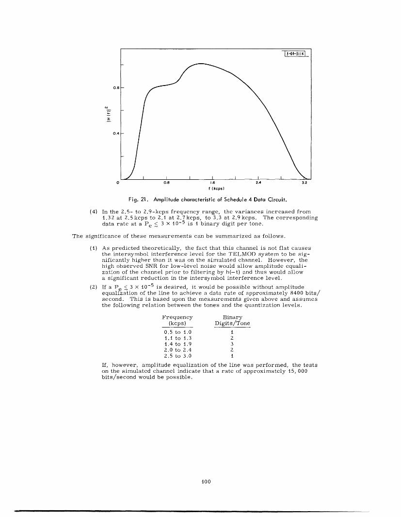
I

0 0.8 1.6 2.4 3.2

f (kcps)

Fig. 21. Amplitude characteristic of Schedule 4 Data Circuit.

(4) In the 2.5- to 2.9-kcps frequency range, the variances increased from1.32 at 2.5 kcps to 2.1 at 2.7kcps, to 3.3 at 2.9 kcps. The correspondingdata rate at a Pe < 3 x 10- 5 is 1 binary digit per tone.

The significance of these measurements can be summarized as follows.

(1) As predicted theoretically, the fact that this channel is not flat causesthe intersymbol interference level for the TELMOD system to be sig-nificantly higher than it was on the simulated channel. However, thehigh observed SNR for low-level noise would allow amplitude equali-zation of the channel prior to filtering by h(-t) and thus would allowa significant reduction in the intersymbol interference level.

(2) If a Pe < 3 x 10 - 5 is desired, it would be possible without amplitudeequalization of the line to achieve a data rate of approximately 8400 bits/second. This is based upon the measurements given above and assumesthe following relation between the tones and the quantization levels.

Frequency Binary(kcps) Digits/Tone

0.5 to 1.0 11.1 to 1.3 21.4 to 1.9 32.0 to 2.4 22.5 to 3.0 1

If, however, amplitude equalization of the line was performed, the testson the simulated channel indicate that a rate of approximately 15, 000bits/second would be possible.

100

_ _I_ I

APPENDIX A

PROOF THAT THE KERNELS OF THEOREMS 1 TO 3 ARE 2

A kernel K(t, s) is said to be an Y2-kernel if 6 5

II KI'- S K2 (t, s) dtds < oo

For the kernel of Theorem 1, it follows that

and thus from the Schwarz inequality

II ·~brT1

h(o - t) h(( - s)

h2((

-T (T1 2h ( - t)

] [Tdoh2( - s) d] dtds

2do- dt]

[ < h2 (o-) d dt]

= h2 (t) dt < oo

which proves that the kernel is 2.' Next, to prove that the kernel of Theorem 2 is £2 define a

function K1/ 2 (t) by

Ki/z(t) - _ H(f) [N(f)] -4/2 ej t df

Then

(t oo /(t ) (- ) d

K(t - s) = K1/2 (t - ) K/2(s - or) du

and, therefore

2II SK=T 5s | K1/Z(t - ) K1/Z2 ( - )

which, from the Schwarz inequality, becomes

I I 12 - ~( (.KI _.

=I&T dtIf 700_ K~i 7 ()do-]

101

dj 2 dt ds

d 12do-J

dt ds

K1/2(s- a) do] dt ds

__I ___· 1_-----11·----�__1_1.--�.�- . .- ~ - - -

Kl2,tK 2 (t

Thus, from Parseval's theorem,

IIK 4 [T I IH(f)l [N(f) ]- dfj Is.oand the kernel

k1/2(t, s) by

is 2' Finally, to prove that the kernel of Theorem 3 is k 2 define a function

- (ht, 'i)T

k (t, s) i(S)i=l I

where

(h t, i)T -

Tt) dc

Yii(- h(a - t) a

and yi(t) and fi are defined as in the proof of Theorem 3. Then

k /2 (t, ar) k/2(s, a) do =(ht i)T (hs I Yj)T

(ht , -i) T (hs I 'i ) T

= R Bi

: oT 1 T

i

h( - t) i ( ) i( P)h( - t) Z i h(p - s) da dp

i=t i

= K(t, s)

1 2 5T T0 0I

T1

0kl/2(t, ) kl/ 2 (s, a)

which becomes, from the Schwarz inequality,

||K|| 2] 5'T J [i k/2 (t, ) de] [fT;o' ;o' [;z, ][;z,2 2

(ht' i)T

i dtji=1

However, it is known 9 8 that

i=

2(ht, i)T

T 5 I H(f) 2

-0 N (f)

102

< o

T 1

Thus,

12do-] dt ds

k1/2(s, o) do] dtds

( i'i 7j)Tti, j J71

Thus,

IIKI zI ?2 T 5 NI(f)l < 0

and the kernel is kZ.

103

__··� _· __ __ _ __·

APPENDIX B

DERIVATION OF ASYMPTOTIC FORM OF ERROR EXPONENTS

This Appendix is concerned with a derivation of the limiting form of the error exponents of

Eqs. (34) to (36) and Eq. (58) for T - . Consider first the standard random coding exponent

given by

R(1) < R < R(0)ET(P) = ( P ) 2 BT(P)

N AX ET(P)R(p) =B , In -

and

N lnX.R

ET(R) = T In BT( )i=l

where

ST N -1+ A.

i=N

and N is chosen to satisfy XN > BT(P) XN+

{Ai} are given by

IH( T ) Xi Xi= Xi- = I

N(T)T

Recall from Sec. IV-C-1 that for large T the

: 1, 2, 3, ... (B-2)

and assume temporarily that IH(f) 2 /N(f) is a continuous monotone nonincreasing function for

f a 0. Also, recall from Fig. 5(a), or observe from Eq. (B-1), that BT(p) is chosen to satisfy

N/2 rN( S 1 z ' T(B3)

2(1 + p) T i [BT(P) H( (B-3)

where now N/2 is the largest integer such that

IH( N )12

N >BT(P)N( T

Observe, as suggested in Fig. B-1, that the quantity

N/2 i) (B-4)

N( (B-4)iT IH()1 2

is an approximation to the area under the curve N(f)/j H(f) I2, while the quantity

104

0O< p < i

0< R< R(1)

(B-i)

BBT(P)

Fig. B-1. Concerning interpretation BT(p)

of Eq.(B-3).

1 2 3 4 N- NT T T 2T 2T

N 12T ' BT(p)

is precisely the area under the line [BT(p)]. Viewed in this manner, it is clear that for arbi-

trarily large T, BT(p) will always be adjusted to make the difference in these two areas equal

to S/z(1 + p). Thus, since N(f)/IH(f) 12 is continuous and therefore Rieman integrable over a

finite interval, 9 and since it is readily shown 9 7 from the definition of a Rieman integral that

when N = 2TW(W > 0)

N/Z-

lim n T 2 T N(f) dfT~ il IH( 2 dH(f) f

it follows that in the limit T -- o, BT(p) or, more simply, B(p) must be chosen to satisfy

2(1 + p) AO [B(p) IH(f) I2 df (B-5)

where W is defined by

H(W) 2 B(p) (B-6)N(W)

From this discussion and Eq. (B-1) it follows that

E(p) lim ET(P) = ( p S2) B(p) 0 p 1 (B-7)

where B(p) is given by Eq. (B-6). Similarly, from Eqs. (B-1), (B-2), and (B-5) if follows that

lim R(p)= lim n (i/T) -r a ln BTP)- P]N(i/T) ZT T P

I H(i/T) 2 N B E(p)= lim T in IN(i/T) - 2-T In B _(p) 0 . p< 1 . (B-8)

T-- T N(i/T) 2T p

From Fig. B- it is clear that for T , N/T W where W is defined by Eq. (B-6). Further-

more, since n (. ) is a continuous function of its argument, it follows from above that

105

� _ 11__1______ 1_�__ 1____11 _· II I

I TT= 11 "·'z

N/2 W 2lim s ln H(i/T) I Z - n I H(f)

Tim T X in N(i/T) N(f)

Thus, from Eq. (B-8),

lim R(p) = ,in (f) 2 df - W lnB(p) - E(p)

= in( df E(p) 0 p 1 . (B-9), l I H(f) 2 E(p)N(f) B(p) p

Equations (B-7) and (B-9) are the desired asymptotic forms when H(f) 2/N(f) is monotonic.

When IH(f) 2 /N(f) is nonmonotonic an analogous derivation shows that for T - oo, B(p) is chosen

so that

S ____ - N(f)] d f12(1 + p) B(p) H(f) 2] d (B-10)

where

W += Nff: H(f)) > B(p)

The corresponding values of E(p) and R(p) are given by

E(p) = (p)2 S B(p) 0 P < + p 2

and

R(p) n IH(f) df E(p) 0 < p ISW 'N(f) B(p) P

which is the result presented in Eqs. (37) and (38).

When 0 .. R.< R(I), it follows from Eq. (B-l) and the previous discussion that

N/2N2 H(i/T)12

lim ET(R) lim i In -RT~o o (R) N(i/T) BT(1)T- T-i- T

=I in N(f) df-R

where B(I) and W are defined by Eq. (B-10). This is the result presented in Eq. (39).

Finally, the similarity of the expurgated bound given in Eq. (58) to the standard bound given

in Eq. (B-i) together with the above results leads directly to the asymptotic form of the ex-

purgated bound presented in Eq. (59).

106

I_ _

APPENDIX C

DERIVATION OF EQUATION (63)

This Appendix proves that the function y(t) which maximizes the functional

-Xx 2 (a) + 5 X(o) x(p)I f'ois a solution of the integral equation

XA(t) = y y(T) K(t - T) dT

where

K(t - T) A Rh(t - T) +

N

h(o - p) + L-=

2PkRh(a - p -k)] p I d

o t < f

N

Z Pk [Rh(t - s + k5) + Rh(t- s -- kJ)]k=i

Following standard variational techniques, 8 5 let x(t) = y(t) + E f(t), where y(t) is the desired

solution, and set

dIlde le=OdFrom E 0q. (C-), this gives

From Eq. (C-1), this gives

e=0 =O - ZXfY() f(r) +

x [Rh(r - ) +

N

k=lk= I

['(o) f(p) + f(o) y(p)]

20kRh( - p - k5)] dp do

However, since Rh(a - ) = Rh(p - a), it follows that

-y() f(p) Rh(a - p) ddp = o so f(cr) y(p) Rh(a- p) d dp

So' S y(U) f(P)0 0

N ' f

PkRh(u--P -k5f)dodp= :' -y(p) f(y)

k=

x kRh(a - p + k 5) d dp

Thus, Eq. (C-3) can be written as

dI | 5eO=2+ Ty(p) K(a - p) dp f(a) du

107

(C-1)

(C-2)

dIde C

and

(C-3)

N

Zk=i

(C-4)

_��_LII(I _·-C---UI-II_�I �---1�I1---- 1 �----- I-- --

5- s

where K(u - p) is defined in Eq. (C-2). Finally, setting

dI = 0

for all f(t) leads to the result that the bracketed quantity in the integrand of Eq. (C-4) must be

zero for all 0 a J< X, i.e., y(t) must be a solution of Eq. (C-2).

108

_ I

APPENDIX D

DERIVATION OF EQUATION (70)

This Appendix proves that if Qo(p) is a polynomial differential operator of order n, if v(t)

has a continuous (n - 1)st derivative and satisfies the boundary conditions of Eq. (68), and if K(t)

is n times differentiable, then

J

so [Qa(P) v(o)] K(t - a) d =

The definition of Qo (p) implies that

n

Qr(p) V((J) = 1, biv(i)(a)

i=O

5-\ V(J

[Q (-p) K(t- )] d.

0.< a< 5-

where

v(i) () d

do1

and

n

Q(s) _ C bisii=O

Thus

So [Q(p) v(c)] K(t - ) d =

n

i=O

v(i)((J) K(t - cr) do

For i > 0, integration by parts and substitution of the boundary conditions of Eq. (68) shows that

- v(i)(c) K(t - i) d = K(t - ci) v (ai) =50 - So v(i-)(o) d K(t- ) da

d=- 5v(i-)(i) d K(t- c) dao

Repeated application of this result leads to

v (ci)() K(t - c) d = (- 1 )i 5) v(c) d- K(t - ) dad~ ~

Thus,

n

3 bi v(i)(ci) K(t - c) do

i=O= v((J) bi(-l )i d K(t -)i dj

5-

:So v(c) [Q (-p) K(t - c] dc

and Eq. (D-1) is proved.

109

(D-1)

_I II__ _ 1_1 __ _______ __^11_1_ 1__11 1_11( l�_li__

_ 1_ _-1^

bi K

APPENDIX E

PROOF OF EVEN-ODD PROPERTY OF NONDEGENERATE EIGENFUNCTIONS

It is desired to prove that all nondegenerate eigenfunctions of the eigenvalue differential

equation

[N(p2 ) - XiD(p2)] vi(t) = 0

Vi(± - ) 0

vi(n-i) = 01 2

are either even or odd functions. Observe

order derivatives and since

d2 k d2 k

tk vit)= Ztk vi(-t)dt dt

-- <t < -2 2 (E- 1)

(E-2)

first that since N(p2) and D(p) contain only even

k = 0, 1,... (E-3)

it follows that if vi(t) is an eigenfunction with eigenvalue Xi , then vi(-t) is also an eigenfunction

with eigenvalue .. Thus, if v (t) is a nondegenerate eigenfunction, there must exist a constant

b such that

vi(t) + bvi(-t) = 0

However, if vie(t) and vio(t) denote the even and odd parts of vi(t), respectively, that is,

vi(t) + v.i(-t)vie( t ) = 2

(E-4)

and

vi(t ) - vi(-t )Vio( t ) = 2

it follows from Eq. (E-4) that (1 - b) vie(t) = -(1 + b) vio(t) and therefore that either b = 1 and

vio(t) = 0 or b = -1 and vie(t) = 0. In other words, a nondegenerate eigenfunction is either even

or odd.

110

I _ __ �

APPENDIX F

OPTIMUM TIME-LIMITED SIGNALS FOR COLORED NOISE

This Appendix presents a generalization of the results of Sec. IV-A to channels with colored

noise. Since a derivation of the results for colored noise follows the previous work quite closely,

only the final results are presented here.

The problem considered is that of choosing a fixed energy, time-limited (to [0, ]) signal to

give at the optimum detector 5 4 output both zero intersymbol interference at t = k, k = 1,

± 2, ... , and a maximum SNR at t = 0. Under the restrictions that h(t) is a lumped parameter

system and N(f) is a rational spectrum, the following result is obtained. As before, let

H(s) H(-s) A N(s 2 )

D(s2 )

let

N(f) A N(s 2 )D(s )s 2=_47r2 f2

2 2-2s -2

and assume that the orders of the polynomials N(s2), D(s2), N(s2), and D(s 2 ) are m, Zn, Zm,

2n, respectively. Then the maximization problem previously outlined leads to the boundary

value differential equation given by

[N(p2) (p2) _iD(p ) N(p)] vi(t ) = 0 0 < t <5

vi(0) = vi(Y) = 0

1 1

The corresponding channel input signals {yi(t)} are

yi(t) Q(p) vi(t) (F-2)

where

n+m

Q(s) n (s - zi)

i=l

z. = ±si i = , ... ,n +m

RHP zeros of D(s 2 ) for i = .. ,n

IRHP zeros of N(s ) for i = n +1, ... H + n

111

_11_1_1_ 1��_11_�� _ _ _

and therefore

Q(s) Q(-s) = cD(s ) N(s Z )

These solutions have the following properties:

(1) The choice zi = s i or zi = -s i in the definition of Q(s) is arbitrary.

Thus, there are 2 n+ m equally valid solutions to the maximization

problem.

(2) The {yi(t)} are orthogonal and may be assumed normalized, i.e.,

in the notation of Sec. IV-A,

(Ti', j)5 = 6ij

This normalization is assumed hereafter.

(3) If K1 (t) is defined as

K (t) Y N(f) ewt df= -n 0 N (f)

and if the generalized inner product is defined as

(f, K1 g)o A S_ f(t) '_ g(C) K(t - ) d(dt

then the {-yi(t)} are "doubly orthogonal" (in the sense of Sec. IV-A) at

the channel output with respect to the generalized inner product, i.e.,

if rij(t) is the channel filter output when yi(t - j) is transmitted, then

(Ar i if i = k and j = 1(rij, Kirki ) =

0 otherwise

(4) The eigenvalues {Xi} are the "generalized energy transfer ratios" of

the filter for the corresponding eigenfunctions, i.e., with rij(t) as

previously defined,

(rio, Krrio)o

3 (Ti' Ti)y

The importance of this result lies in the fact that the SNR at the

optimum detector output at t = 0 is given by

{X(f) H(f) 12N(f) df

when x(t) is the transmitted signal. Thus, -y(t) is the solution to

the original maximization problem.

112

_____ _._ __I ___I_

ACKNOWLEDGMENT

I would like to express my sincere appreciation to Professor J.M. Wozencraft

for his guidance and encouragement during this work. The opportunity of

working closely with him for the past two years has proved to be the most

stimulating and rewarding experience in my doctoral program. Also, I wish

to thank my readers, Professor R. G. Gallager and Professor W. M. Siebert, for

numerous helpful discussions, and to acknowledge the important role in this

work of the bounding techniques developed by Professor Gallager.

I also wish to express my thanks to a number of people at Lincoln Laboratory

who contributed significantly to this work. In particular, I would like to

thank both P. E. Green, Jr., who provided the initial encouragement to work

on this problem as well as the technical support that made the experimental

program possible, and P.R. Drouilhet who providedvaluable guidance both in

the construction of the experimental equipment and in numerous discussions

throughout the course of this work.

113

_ _· ___111 1-1111 -.I1_ I ---

REFERENCES

1. A.B. Clark, "Telephone Transmission Over Long Cable Circuits," Bell System Tech. J. 2, 67(1923).

2. O.E. Buckley, "High-Speed Ocean Cable Telegraphy," Ibid. 7, 225 (1928).

3. J.R. Carson, "Theory of Transient Oscillations of Electrical Networks and Transmission Systems,"Trans. AI EE (February 1919).

4. , "The Building Up of Sinusoidal Currents in Long Periodically Loaded Lines," BellSystem Tech. J. 3, 558 (1924).

5. H. Nyquist, "Certain Factors Affecting Telegraph Speed," Ibid. 3, 324 (1924).

6. , "Certain Topics in Telegraph Transmission Theory," Trans. AIEE 47, 617 (1928).

7. S.P. Mead, "Phase Distortion and Phase Distortion Correction," Bell System Tech. J. 7, 195(1928).

8. H. Nyquist and S. Brand, "Measurement of Phase Distortion," Ibid. 9, 522 (1930).

9. O.J. Zobel, "Distortion Correction in Electrical Circuits with Constant Resistance RecurrentNetworks," Ibid. 7, 438 (1928).

10. J.V. Harrington, P. Rosen, and D.A. Spaeth, "Some Results on the Transmission of Pulses overTelephone Lines," Proceedings of the Symposium on Information Networks (Polytechnic Instituteof Brooklyn, Brooklyn, N.Y., 1954), pp. 115-130.

11. K.E. Perry, "Phone Line Data Transmission Systems," Group Report 24-54, Lincoln Laboratory,M. I. T. (September 1955), H-106.

12. P. Mertz, "Transmission Line Characteristics and Effects on Pulse Transmission," Proceedings ofthe Symposium on Information Networks (Polytechnic Institute of Brooklyn, Brooklyn, N.Y.,1954), pp. 85 -1 14 .

13. E.D. Sunde, "Theoretical Fundamentals of Pulse Transmission," Bell System Tech. J. 33, 721(1954).

14. A.W. Horton and H.E. Vaughn, "Transmission of Digital Information Over Telephone Circuits,"Ibid. 34, 511 (1955).

15. W.D. Cannon, "Delay Distortion Correction," Trans. AIEE Commun. Electron. No. 23, 107(1956).

16. B. P. Bogert, "Demonstrations of Delay Distortion Correction by Time-Reversal Techniques'," Trans.IRE, PGCS CS-5, 2 (1957).

17. P. Mertz and D. Mitchell, "Transmission Aspects of Data Transmission Service Using Private LineVoice Telephone Channels," Bell System Tech. J. 36, 1451 (1957).

18. A.D. Fowler and R.A. Gibby, "Assessment of Effects of Delay Distortion in Data Systems," Trans.AIEE Commun. Electron., No. 40, 918 (1959).

19. R.G. Enticknap and E.F. Schuster, "SAGE Data System Considerations," Ibid., No. 40, 824(1959).

20. E.D. Sunde, "Ideal Binary Pulse Transmission by AM and FM," Bell System Tech. J. 38, 1357(1959).

21. R.G. Enticknap, "The Testing of Digital Data Transmission Channels and Circuits," Proceedingsof the AIEE National Electronics Conference (Chicago, 1960), Vol. XVI, pp. 66-71.

22. E.J. Hofmann and G.E. Masters, "Error Statistics on Dual A-1 Digital Data Transmission Circuitsfrom Kingston, New York to Cape Canaveral, Florida," Group Report 2G-25-4, Lincoln Labora-tory, M.I.T. (6 June 1958), DDC 244772, H-185.

23. L.A. Weber, "A F-M Digital Subset for Data Transmission Over Telephone Lines," Trans. AIEECommun. Electron., No. 40, 867 (1959).

114

_I _ _ _�

24. G. Holland and J.C. Myrick, "A 2500-Baud Time-Sequential Transmission System for Voice-Frequency Wire Line Transmission," Trans. IRE, PGCS CS-7, 180 (1959).

25. K.E. Perry, "An Error-Correcting Encoder and Decoder for Phone Line Data," IRE Wescon Con-vention Record (San Francisco, 1959), Part 4, pp. 21-26.

26. E.J. Hofmann, "Error Statistics on Dual A-1 Digital Data Transmission Circuits from Lexington,Massachusetts to So. Truro, Massachusetts," Group Report 2G-25-12, Lincoln Laboratory, M.I.T.(February 1959), H-169.

27. E.J. Hofmann, P.L. Grant, and E.H. Harvey, "Error Statistics on the Collins Kineplex OverVarious Media," Group Report 25G-0024, Lincoln Laboratory, M.I.T. (12 January 1961), DDC251447, H-257.

28. E. J. Hofmann and P.L. Grant, "Error Statistics on a Long-Haul Looped Telephone Circuit Utiliz-ing the Milgo Data System," Group Report 25G-0010, Lincoln Laboratory, M.I.T. (17 June 1960),DDC 240820, H-134.

29. J.L. Hollis, "Digital Data Fundamentals and the Two Level Vestigial Sideband System for VoiceBandwidth Circuits," IRE Wescon Convention Record (San Francisco, 1960), Part 5, pp. 132-145.

30. R.A. Gibby, "An Evaluation of AM Data System Performance by Computer Simulation," BellSystem Tech. J. 39, 55 (1960).

31. H.L. Yudkin, "Some Results in the Measurement of Impulse Noise on Telephone Circuits;' Pro-ceedings of the AIEE National Electronics Conference (Chicago, 1960), Vol. XVI, pp. 222-231.

32. R.P. Pfeiffer and H.L. Yudkin, "Impulse Noise on an H-44 Telephone Circuit Looped fromLexington, Massachusetts via West Haven, Connecticut," Group Report 25G-0012, LincolnLaboratory, M. I.T. (April 1960), DDC 236232, H-79.

33. A.A. Alexander, R.M. Gryb, and D.W. Nast, "Capabilities of the Telephone Network for DataTransmission," Bell System Tech. J. 39, 431 (1960).

34. H.L. Yudkin, "Experiments in the Improvement of the Impulse Response of Telephone Circuits,"Group Report 25G-4, Lincoln Laboratory, M.I.T. (27 November 1961), DDC 269557, H-373.

35. B. Reiffen, W.G. Schmidt, and H.L. Yudkin, "The Design of an 'Error-Free' Transmission Systemfor Telephone Circuits," Trans. AIEE Commun. Electron., No. 55, 224 (1961).

36. E. J. Hofmann, "Error Statistics Utilizing the Code Translation Data System Over Various Media,"Group Report 25G-0026, Lincoln Laboratory, M. I.T. (28 March 1961), DDC 254037, H-278.

37. E. Hopner, "Phase Reversal Data Transmission for Switched and Private Telephone Line Applica-tions," IBM J. Research Develop. 5, 93 (1961).

38. J.E. Toeffler and J. N. Buterbaugh, "The HC-270, A Four-Phase Digital Transceiver," SelectedWescon Papers, No. 36/1 (1961).

39. A.B. Fontaine and R.G. Gallager, "Error Statistics and Coding for Binary Transmission overTelephone Circuits," Proc. IRE 49, 1059 (1961).

40. P. Mertz, "Model of Impulse Noise for Data Transmission;' Trans. IRE, PGCS CS-9, 130 (1961).

41. E.D. Sunde, "Pulse Transmission by AM, FM, and PM in the Presence of Phase Distortion," BellSystem Tech. J. 40, 353 (1961).

42. G. Comstock, "Low Cost Terminals Triple Phone TV Link Data Rates," Electronic Design 11, 8(1963).

43. I.L. Lebow, et al., "Application of Sequential Decoding to High-Rate Data Communication ona Telephone Line," Trans. IEEE, PTGIT IT-9, 124 (1963).

44. Business Week, "New UNIVAC Device Provides an Inexpensive Way to Link Some of Its Com-puters by Telephone" (9 November 1963), p. 150.

45. Ibid., "New Challenge to IBM" (7 December 1963), p. 30.

46. G. Burck, "The Boundless Age of the Computer," Fortune (March 1964), p. 230.

47. U.S. News and World Report, "What's Coming Tomorrow from Today's Telephones" (9 March 1964),pp. 60-64.

115

�_II� __ -----II·U·IIIIPIII^��·-

48. M.A. Rappeport, "Four Phase Data Systems Evaluation by Computer Simulation" (unpublished).

49. M.L. Doelz, E.T. Heald, and D.L. Martin, "Binary Data Transmission Techniques for Linear Sys-tems," Proc. IRE 45, 656 (1957).

50. K.E. Perry and J.M. Wozencraft, "SECO: A Self-Regulating Error-Correcting Coder-Decoder,"Trans. IRE, PGIT IT-8, 128 (1962).

51. R.M. Fano, Transmission of Information (M. I.T. Press, Cambridge, Mass., and Wiley, NewYork, 1961).

52. J.M. Berger and B.M. Mandelbrot, "A New Model for Error Clustering in Telephone Circuits,"IBM J. Research Develop. 7, 224 (1963).

53. C.E. Shannon, "Probability of Error for Optimal Codes in a Gaussian Channel," Bell System Tech.J. 38, 611 (1959).

54. C.W. Helstrom, Statistical Theory of Signal Detection (Pergamon Press, New York, 1960).

55. P. Holmos, Finite Dimensional Vector Spaces (Van Nostrand, Princeton, N.J., 1958).

56. E.J. Baghdady, editor, Lectures on Communication Theory (McGraw-Hill, New York, 1961).

57. G. Sansone, Orthogonal Functions (Interscience Publishers, New York, 1959).

58. G.E. Valley, Jr., and H. Wallman, Vacuum Tube Amplifiers, Radiation Laboratory Series, M. I.T.,Vol. 18 (McGraw-Hill, New York, 1948).

59. E. Arthurs and H. Dym, "On the Optimum Detection of Digital Signals in the Presence of WhiteGaussian Noise - A Geometric Interpretation and a Study of Three Basic Data Transmission Sys-tems,"' Trans. IRE, PGCS CS-10, 336 (1962).

60. W.B. Davenport, Jr., and W.L. Root, An Introduction to the Theory of Random Signals and Noise(McGraw-Hill, New York, 1958).

61. D.C. Youla, "The Use of the Method of Maximum Likelihood in Estimating Continuous-ModulatedIntelligence Which Has Been Corrupted by Noise'" Trans. IRE, PGIT IT-3, 90 (1954).

62. N. Dunford and J.T. Schwartz, Linear Operators, Part I1 (Interscience Publishers, New York,1963).

63. E.R. Lorch, Spectral Theory (Oxford University Press, New York, 1962).

64. R. Courant and D. Hilbert, Methods of Mathematical Physics (Interscience Publishers, New York,1958).

65. F.G. Tricomi, Integral Equations (Interscience Publishers, New York, 1957).

66. B. Friedman, Principles and Techniques of Applied Mathematics (Wiley, New York, 1956).

67. J.L. Holsinger, "Vector Representation of Time Continuous Channels with Memory," QuarterlyProgress Report 71, Research Laboratory of Electronics, M. I.T. (15 October 1963), pp. 193-202.

68. E. C. Titchmarsh, Introduction to the Theory of Fourier Integrals (Oxford University Press, New York,1959). (See Lemma 3, p. 324.)

69. T.M. Apostol, Mathematical Analysis (Addison-Wesley, Reading, Mass., 1957).

70. R. Price, private communication.

71. J.H.H. Chalk, "The Optimum Pulse-Shape for Pulse Communication," Proc. IEEE 97, 88 (1950).

72. H. J. Landau and H.O. Pollak, "Prolate Spheroidal Wave Functions, Fourier Analysis and Un-certainty- 11: The Dimension of the Space of Essentially Time- and Band-Limited Signals,"Bell System Tech. J. 41, 1295 (1962).

73. D. Slepian and H. O. Pollak, "Prolate Spheriodal Wave Functions, Fourier Analysis and Uncer-tainty - I," Bell System Tech. J. 40, 40 (1961).

74. R. G. Gallager, "A Simple Derivation of the Coding Theorem," Quarterly Progress Report 69,Research Laboratory of Electronics, M. I.T. (15 April 1963), pp. 154-157.

116

----� ---- --- I

75. R. G. Gallager, "A Simple Derivation of the Coding Theorem and Some Applications," Trans.IEEE, PTGIT IT-11, No. 1 (1965).

76. J.L. Holsinger, "An Error Bound for Fixed Time Continuous Channels with Memory," QuarterlyProgress Report 72, Research Laboratory of Electronics, M. I. T. (15 January 1964), pp. 198-207.

77. , "An Improved Low-Rate Error Bound for Fixed Time Continuous Channels withMemory," Quarterly Progress Report 73, Research Laboratory of Electronics (15 April 1964),pp. 141-147.

78. G.H. Hardy, J.E. Littlewood, and G. Polya, Inequalities (Cambridge University Press, London,1959), Theorem 190.

79. H.G. Eggleston, Convexity, Cambridge Tracts in Mathematics and Mathematical Physics, No. 47(Cambridge University Press, London, 1958).

80. H.W. Kuhn and A.W. Tucker, "Nonlinear Programming," Second Berkeley Symposium on Mathe-matical Statistics and Probability (University of California Press, Berkeley, 1951), p. 486,Theorem 3.

81. J.M. Wozencraft and R.S. Kennedy, "Coding and Communication," URSI Spring Conference (1963).

82. J.M. Wozencraft and B. Reiffen, Sequential Decoding (Wiley, New York, 1961).

83. R.G. Gallager, Low-Density Parity-Check Codes (M. I.T. Press, Cambridge, Mass., 1963).

84. J.L. Massey, "Threshold Decoding," Technical Report 410, Research Laboratory of Electronics,M.I. T. (5 April 1963).

85. F.B. Hildebrand, Methods of Applied Mathematics (Prentice-Hall, Englewood Cliffs, N.J., 1952).

86. T. Muir, A Treatise on the Theory of Determinants (Dover Publications, New York, 1960),Chapter XI.

87. I. Gerst and J. Diamond, "The Elimination of Intersymbol Interference by Input Signal Shaping,"Proc. IRE 49, 1195 (1961).

88. I.S. Sokolnikoff and R.M. Redheffer, Mathematics of Physics and Modern Engineering (McGraw-Hill, New York, 1958).

89. F.G. Brauer, "Singular Self-Adjoint Boundary Value Problem for the Differential EquationLx = XMx," PhD Thesis, Department of Mathematics, M. I.T. (1956).

90. J.C. Hancock and H. Schwarzlander, "Certain Optimum Signaling Waveforms For Channels withMemory," Technical Report No. TR-EE64-11, Purdue University, Lafayette, Indiana (June 1964).

91. J.S. Richters, "Minimization of Error Probability for a Coaxial Cable Pulse Transmission System,"MSc Thesis, Department of Electrical Engineering, M. I. T. (June 1963).

92. D.C. Youla, "The Solution of a Homogeneous Wiener-Hopf Integral Equation Occurring in the Ex-pansion of Second-Order Stationary Random Functions'" Trans. IRE, PGIT IT-3, 187 (1956).

93. D.W. Tufts, "Matched Filters and Intersymbol Interference," Technical Report No. 345, CruftLaboratory, Harvard University (20 July 1961).

94. P.M. Woodward, Probability and Information Theory with Applications to Radar (Pergamon Press,New York, 1960).

95. J. Capon, "Asymptotic Eigenfunctions and Eigenvalues of a Homogeneous Integral Equation:'Trans. IRE, PGIT IT-8, 2 (1962).

96. M. Rosenblatt, "Asymptotic Behavior of Eigenvalues for a Class of Integral Equations with Trans-lation Kernels," Proceedings of the Symposium on Time Series Analysis, Brown University (Wiley,New York, 1963), Chapter 21.

97. G.B. Thomas, Jr., Calculus and Analytic Geometry (Addison-Wesley, Reading, Mass., 1958).

98. E. J. Kelly, et al., "The Detection of Radar Echoes in Noise," J. Soc. Indust. Appl. Math. 8,309 (1960).

99. L.B.W. Jolley, Summation of Series (Dover Publications, New York, 1961).

117

_111------�11.-11_-1 .-·-..11_1_---�- -�li^ .^---l^^-·-. ---�--CI- �--· -1111 _ _ -- _�

JOINT SERVICES DISTRIBUTION LIST

Department of Defense

Dr Edward M. ReilleyAsst Director (Research)Ofc of Defense Res & EngDepartment of DefenseWashington, D.C. 20301

Dr James A. WardOffice of Deputy Director (Research

and Information Rm 3D1037Department of DefenseThe PentagonWashington, D.C. 20301

DirectorAdvanced Research Projects AgencyDepartment of DefenseWashington, D.C. 20301

Mr Charles Yost, DirectorFor Materials SciencesAdvanced Research Projects AgencyDepartment of DefenseWashington, D.C. 20301

Defense Documentation CenterAttn: TISIACameron Station, Bldg 5Alexandria, Virginia 22314

DirectorNational Security AgencyAttn: C3/TDLFort George G. Meade, Maryland 20755

Department of the Army

Chief of Research and DevelopmentHeadquarters, Department of the ArmyAttn: Physical Sciences Division P&EWashington, D.C. 20310

Research Plans OfficeU. S. Army Research Office3045 Columbia PikeArlington, Virginia 22204

Commanding OfficerForeign Service & Technology CenterArlington HallArlington, Virginia

Commanding GeneralU. S. Army Materiel CommandAttn: AMCRD-RS-PE-EWashington, D.C. 20315

Commanding GeneralU. S. Army Strategic Communications

CommandWashington, D.C. 20315

Commanding GeneralU.S. Army Materials Research AgencyWatertown ArsenalWatertown, Massachusetts 02172

Commanding OfficerU. S. Army Ballistics Research LaboratoryAttn: V.W. RichardsAberdeen Proving GroundAberdeen, Maryland 21005

CommandantU. S. Army Air Defense SchoolAttn: Missile Sciences Division, C&S Dept.P.O. Box 9390Fort Bliss, Texas 79916

Commanding GeneralU.S. Army Missile CommandAttn: Technical LibraryRedstone Arsenal, Alabama 35809

Commanding GeneralFrankford ArsenalAttn: SMUFA-1310 (Dr Sidney Ross)Philadelphia, Pennsylvania 19137

U.S. Army Munitions CommandAttn: Technical Information BranchPicatinney ArsenalDover, New Jersey 07801

Commanding OfficerHarry Diamond LaboratoriesAttn: Mr Berthold AltmanConnecticut Avenue and Van Ness Street N. W.Washington, D.C. 20438

Commanding OfficerHarry Diamond LaboratoriesAttn: Dr R. T. Young

Electron Tubes DivisionConnecticut Avenue and Van Ness Street N. W.Washington, D.C. 20438

Commanding OfficerU. S. Army Security AgencyArlington HallArlington, Virginia 22212

Commanding OfficerU. S. Limited War LaboratoryAttn: Technical DirectorAberdeen Proving GroundAberdeen, Maryland 21005

JOINT SERVICES DISTRIBUTION LIST (continued)

Commanding OfficerHuman Engineering LaboratoriesAberdeen Proving GroundMaryland 21005

DirectorU. S. Army Engineer Geodesy,

Intelligence and MappingResearch and Development AgencyFort Belvoir, Virginia 22060

CommandantU.S. Army Command and General Staff

CollegeAttn: SecretaryFort Leavenworth, Kansas 66207

Dr. H. Robl, Deputy DirectorU. S. Army Research Office (Durham)P.O. Box CM, Duke StationDurham, North Carolina 27706

Commanding OfficerU. S. Army Research Office (Durham)Attn: CRD-AA-IP (Richard O. Ulsh)P.O. Box CM, Duke StationDurham, North Carolina 27706

Commanding GeneralU. S. Army Electronics CommandAttn: AMSEL-SCFort Monmouth, New Jersey 07703

DirectorU. S. Army Electronics LaboratoriesAttn: Dr S. Benedict Levin, Director

Institute for Exploratory ResearchFort Monmouth, New Jersey 07703

DirectorU. S. Army Electronics LaboratoriesAttn: Mr Robert O. Parker, Executive

Secretary JSTAC (AMSEL-RD-X)Fort Monmouth, New Jersey 07703

SuperintendentU. S. Army Military AcademyWest Point, New York 10996

The Walter Reed Institute of ResearchWalter Reed Army Medical CenterWashington, D.C. 20012

DirectorU. S. Army Electronics LaboratoriesFort Monmouth, New Jersey 07703Attn: AMSEL-RD-DR NE SS

X NO PEXE NP PRXC SA PFXS SE GFNR SR ADT

FU# 1

Commanding OfficerU. S. Army Electronics R&D ActivityFort Huachuca, Arizona 85163

Commanding OfficerU. S. Army Engineers R&D LaboratoryAttn: STINFO BranchFort Belvoir, Virginia 22060

Commanding OfficerU. S. Army Electronics R&D ActivityWhite Sands Missile RangeNew Mexico 88002

DirectorHuman Resources Research OfficeThe George Washington University300 N. Washington StreetAlexandria, Virginia 22314

Commanding OfficerU. S. Army Personnel Research OfficeWashington, D.C.

Commanding OfficerU.S. Army Medical Research LaboratoryFort Knox, Kentucky

Department of the Air Force

DirectorAir University LibraryMaxwell A. F. Base, Alabama

CommanderAir Force Office of Scientific ResearchWashington 25, D.C.Attn:-SREE

Department of The Air ForceHeadquarters-United States Air ForceWashington 25, D.C.Attn: AFTAC/TD- 1

Dr. Harvey E. Savely, SRLAir Force Office of Sci. Res.Office of Aerospace Research, USAFWashington 25, D.C.

Mr. C.N. HasertScientific Advisory BoardHq, USAFWashington 25, D.C.

-�-X-�LIIII�I· -� --- �I I� I_ -·-.�I-� II-- I

JOINT SERVICES DISTRIBUTION LIST (continued)

APGC (PGBAP- 1)Elgin Air Force BaseFlorida 32542

AFETR(AFETR Tech. Library MU-135)Patrick Air Force BaseCocoa, Florida

Air Force Cambridge Res. Lab.L. G. Hanscom FieldBedford, Massachusetts 01731Attn: CRDM, Mr. Herskovitz

Commander, AFCRLAttn: C.P. Smith (CRBS)L.G. Hanscom FieldBedford, Massachusetts

Dr. L. C. BlockAFCRL (CROV)L. G. Hanscom FieldBedford, Massachusetts

AFCRLOffice of Aerospace Res., USAFBedford, Mass.Attn: CRDA

Mr. Rocco H. Urbano, ChiefAFCRL, Appl. Math. BranchData Sciences LaboratoryLaurence G. Hanscom FieldBedford, Massachusetts

AFCRL (CRFE-Dr. Nicholas Yannoni)L. G. Hanscom FieldBedford, Massachusetts

S. H. SternickAerospace Comm. - Attn: ESNCWaltham Federal Center424 Trapelo RoadWaltham, Massachusetts 02154

Rome Air Dev. Center (RAWL, H. Webb)Griffiss Air Force BaseNew York 13442

Systems Engineering GroupDeputy for Systems Eng'g., SEPRRDirectorate of Tech. Pubs. and Specs.Wright-Patterson AFB, OHIO 45433

Aeronautical Systems DivisionAttn: ASRPE, Mr. Robt. CooperWright-Patterson AFC, Ohio 45433

Aeronautical Systems DivisionAttn: ASRPP-20 (Mr. Don R. Warnock)Wright-Patterson AFB, Ohio 45433

AFALAVR (L)Wright-Patterson AFBOhio 45433

Dr. H. H. KurzwegDirector Research - OARTNASAWashington, D.C. 20546

Systems Engineering Group (RTD)Attn: SEPIRWright-Patterson AFB, Ohio 45433

AFAL (AVTE)Wright-Patterson AFBOhio 45433

Mr. Roland ChaseNational Aeronautics & Space Administration1512 H Street, N.W.Washington 25, D.C.

Professor Arwin DougalUniversity of TexasEE DepartmentAustin, Texas

Honorable Alexander H. FlaxAsst Secretary of the Air Force (R&D)Office of the Secretary of the Air ForceWashington 25, D.C.

Professor Nicholas GeorgeCalifornia Institute of TechnologyEE DepartmentPasadena, California

Dr. Lowell M. HollingsworthAFCRLL.G. Hanscom FieldBedford, Massachusetts

Dr. Zohrab KaprielianUniversity of Southern CaliforniaUniversity ParkLos Angeles 7, California

_ I

JOINT SERVICES DISTRIBUTION LIST (continued)

Dr. John M. IdeNational Science FoundationWashington 25, D.C.

Lt Col Edwin M. MyersHeadquarters USAF (AFRDR)Washington 25, D.C.

Professor Wm. H. RadfordDirector, Lincoln LaboratoriesLexington, Massachusetts

Brig Gen B.G. Holzman, USAF (Ret.)Electronics Research Center, NASA30 Memorial DriveCambridge, Mass.

Dr. R. L. SproullDirector, Advanced Research Projects

A gencyWashington 25, D.C.

Brigadier General J. T. StewartDirector of Science & TechnologyDeputy Chief of Staff (R&D)USA FWashington 25, D.C.

Mr. James TippettNational Security AgencyFort Meade, Maryland

Dr. H. HarrisonNASA (Code RRE)Fourth and Independence StreetsWashington, D.C. 20546

AECCiv of Tech Info ExtP.O. Box 62Oak Ridge, Tenn.

AFRST (SC/EN)Lt Col L. StoneRm 4C 341The PentagonWashington, D.C. 20301

U. S. Atomic Energy CommissionLibraryGaithersburg, Md. 20760

ARL (ARD/Col R. E. Fontana)Wright-Patterson AFB,Ohio 45433

Office of Research AnalysesAttn: Col K.W. GallupHolloman AFB, NMex 88330

AFCRL (CRXL)L. G. Hanscom FldBedford, Mass 01731

Frank J. Seiler Rsch LabLibraryUSAF Academy, Colo 80840

ARL (AROL)Wright-Patterson AFB,Ohio 45433

Office of Research AnalysesLibraryHolloman AFB, NMex 88330

LOOAR (Library)AF Unit Post OfficeLos Angeles, Calif 90045

Churchill Research RangeLibraryFort ChurchillManitoba, Canada

Los Alamos Scientific LabAttn: Technical LibraryLos Alamos, NMex 87544

Battelle Memorial InstituteTechnical Library505 King AvenueColumbus, Ohio 43201

John Crerar Library35 West 33rd St.Chicago, Ill.

Linda Hall Library5109 Cherry St.Kansas City, Mo.

National Science FoundationLibrary1951 Constitution Ave., N. W.Washington, D.C. 20550

I_ III�_I I��_�-IIIIl--.t-�-�- ---̂ --II-- -I

JOINT SERVICES DISTRIBUTION LIST (continued)

Johns Hopkins UniversityApplied Physics Lab LibraryWhite OakSilver Spring, Md. 20910

Stanford Research InstituteLibrary820 Mission St.South Pasadena, Calif. 91030

Southwest Research InstituteLibrary8500 Culebra RoadSan Antonio, Texas

ARPA, Tech Info OfficeThe PentagonWashington, D.C. 20301

DDR&E (Tech Library)Rm 3C 128The PentagonWashington, D.C. 20301

Industrial College of theArmed Forces

Attn: LibraryWashington, D.C.

AFIT (MC LI)Tech LibraryWright-Patterson AFBOhio 45433

AUL 3T-9663Maxwell AFB, Ala 36112

USAFA (DLIB)USAF Academy, Colorado 80840

AFSC (Tech Library)Andrews AFBWashington, D.C. 20331

ASD (Tech Library)Wright- Patterson, AFBOhio 45433

BSD (Tech Library)Norton AFB, Calif 92409

ESD (ESTI)L. G. Hanscom Field, F172Bedford, Mass 01731

RTD (Tech Library)Bolling AFC, D.C. 20332

AFFTC (Tech Library)Edwards AFB, Calif 93523

AFMDC (Tech Library)Holloman AFB, NMex 88330

AFWL (WLIL, Tech Library)Kirtland AFB, NMex 87117

APGC (Tech Library)Eglin AFB, Fla 32542

AEDC (Tech Library)Arnold AFS, Tenn 37389

RADC (Tech Library)Griffiss AFB, N.Y. 13442

DirectorNational Aeronautical EstablishmentOttawa, Ontario, Canada

CIAOCR/LY/IASIH 129 HqWashington, D.C. 20505

National Defense LibraryHeadquartersOttawa, Ontario, Canada

Technical LibraryWhite Sands Missile RangeNMex 88002

NASA/AFSS/1 FOB6Tech Library, Rm 60084Washington, D.C. 20546

Space Systems DivisionLos Angeles Air Force StationAir Force Unit Post OfficeLos Angeles, California 90045Attn: SSSD

U.S. Regional Science Office/LAOARU.S. EmbassyAPO 676New York, N.Y.

Ames Rsch Center (NASA)Technical LibraryMoffett Field, Calif 94035

----- - --�-- --- I _� _�

JOINT SERVICES DISTRIBUTION LIST (continued)

High Speed Flight Center (NASA)Technical LibraryEdwards AFB, Calif 93523

Goddard Space Flight Center (NASA)Greenbelt, Md. 20771

Geo. C. Marshall Space FlightCenter (NASA)

Redstone Arsenal, Ala 35808

Lewis Research Center (NASA)Technical Library21000 Brookpark RoadCleveland, Ohio

Aerospace Corp (Tech Library)P.O. Box 95085Los Angeles, Calif 90045

Rand Corporation1700 Main St.Santa Monica, Calif 90401

CommanderAir Force Cambridge Research LaboratoriesOffice of the Scientific DirectorL. G. Hanscom FieldBedford, Massachusetts

CommanderAir Force Systems CommandOffice of the Chief ScientistAndrews AFB, Maryland

CommanderResearch & Technology DivisionAFSCOffice of the Scientific DirectorBolling AFB 25, D.C.

CommanderRome Air Development CenterAFSCOffice of the Scientific DirectorGriffiss AFB, Rome, New York

Carnegie Institute of TechnologyScience & Engineering Hunt LibrarySchenley ParkPittsburgh, Pa. 15213

California Institute of TechnologyAeronautics Library1201 East Calif St.Pasadena 4, Calif

AVCO Research LabLibrary2385 Revere Beach ParkwayEverett, Mass 02149

Dr. G. E. Knausenbergerc/o Hq. Co. Munich PostAPO 09407New York, N. Y.

CommanderSpace Systems Division (AFSC)Office of the Scientific DirectorInglewood, California

CommanderAerospace Systems DivisionAFSCOffice of the Scientific DirectorWright-Patterson AFB, Ohio

CommanderAerospace Research Laboratories (OAR)Office of the Scientific DirectorWright-Patterson AFB, Ohio

Department of the Navy

Dr. Arnold Shostak, Code 427Head, Electronics BranchPhysical Sciences DivisionDepartment of the NavyOffice of Naval ResearchWashington, D.C. 20360

Chief of Naval Research, Code 427Department of the NavyWashington, D.C. 20360

Chief, Bureau of WeaponsDepartment of the NavyWashington, D.C. 20360

Chief, Bureau of ShipsDepartment of the NavyWashington, D.C. 20360Attn: Code 680

CommanderU. S. Naval Air Development CenterJohnsville, PennsylvaniaAttn: NADC Library

.. ~ ~~~ , -- 11_ 11111.- ·. 1_, 1 -·----·1- - w

JOINT SERVICES DISTRIBUTION LIST (continued)

LibraryU. S. Navy Electronics LaboratorySan Diego, California 92152

Commanding OfficerU. S. Navy Underwater SoundFt TrumbullNew London, Connecticut

Laboratory

DirectorNaval Research LaboratoryWashington, D.C. 20390

Commanding OfficerOffice of Naval Research Branch OfficeNavy 100, Fleet P.O. Box 39New York, New York

Chief of Naval OperationsPentagon OP 07TWashington, D. C.

Commanding OfficerOfficer of Naval Research Branch Office495 Summer StreetBoston, Massachusetts 021 10

CommanderNaval Ordnance LaboratoryWhite Oak, MarylandAttn: Technical Library

U. S. Navy Post Graduate SchoolMonterey, CaliforniaAttn: Electrical Engineering Department

_ _� �__