Models for Nonideal Reactors - University of Michiganelements/5e/18chap/Fogler_Web_Ch18.pdf · 18-2 Models for Nonideal Reactors Chapter 18 18.1 Some Guidelines for Developing Models

18-1

18

Models for Nonideal

Reactors

Success is a journey, not a destination.—Ben Sweetland

Use the RTD toevaluate

parameters.

Overview. Not all tank reactors are perfectly mixed nor do all tubular reac-tors exhibit plug-flow behavior. In these situations, some means must beused to allow for deviations from ideal behavior. Chapter 17 showed howthe RTD was sufficient if the reaction was first order or if the fluid waseither in a state of complete segregation or maximum mixedness. We usethe segregation and maximum mixedness models to bound the conversionwhen no adjustable parameters are used. For non-first-order reactions in afluid with good micromixing, more than just the RTD is needed. These situ-ations compose a number of reactor analysis problems and cannot beignored. For example, we may have an existing reactor in storage and wantto carry out a new reaction in that reactor. To predict conversions and prod-uct distributions for such systems, a model of reactor flow patterns and/orRTD is necessary.

After completing this chapter you will be able to• Discuss guidelines for developing one- and two-parameter models

(Section 18.1).• Use the tanks-in-series (T-I-S) one-parameter model to predict

conversion (Section 18.2).• Use the dispersion one-parameter model to predict conversion

(Section 18.3).• Use the RTD to evaluate the model parameters (e.g., Da, n) for

one-parameter models.• Develop equations to model flow, dispersion, and reaction (Section

18.4).

Fogler_Web_Ch18.fm Page 1 Saturday, March 18, 2017 5:30 PM

18-2

Models for Nonideal Reactors Chapter 18

18.1 Some Guidelines for Developing Models

The overall goal is to use the following equation

The choice of the particular model to be used depends largely on the engineer-ing judgment of the person carrying out the analysis. It is this person’s job tochoose the model that best combines the conflicting goals of mathematicalsimplicity and physical realism. There is a certain amount of art in the develop-ment of a model for a particular reactor, and the examples presented here canonly point toward a direction that an engineer’s thinking might follow.

For a given real reactor, it is not uncommon to use all the models dis-cussed previously to predict conversion and then make comparisons. Usually,the real conversion will be

bounded

by the model calculations.The following guidelines are suggested when developing models for non-

ideal reactors:

1.

The model must be mathematically tractable

. The equations used to describea chemical reactor should be able to be solved without an inordinateexpenditure of human or computer time.

2.

The model must realistically describe the characteristics of the nonideal reactor

.The phenomena occurring in the nonideal reactor must be reason-ably described physically, chemically, and mathematically.

3.

The model should not have more than two adjustable parameters

. This con-straint is often used because an expression with more than twoadjustable parameters can be fitted to a great variety of experimentaldata, and the modeling process in this circumstance is nothing morethan an exercise in curve fitting. The statement “Give me four adjust-able parameters and I can fit an elephant; give me five and I caninclude his tail!” is one that I have heard from many colleagues.Unless one is into modern art, a substantially larger number of adjust-able parameters is necessary to draw a reasonable-looking elephant.

1

A one-parameter model is, of course, superior to a two-parametermodel if the one-parameter model is sufficiently realistic. To be fair,however, in complex systems (e.g., internal diffusion and conduction,

1

J. Wei,

CHEMTECH

, 5, 128 (1975).

• Discuss dispersion and reaction in tubular reactors (Section 18.6).• Suggest combinations of ideal reactors to model the nonideal reac-

tor to predict conversion (Section 18.7).• Use RTD data to evaluate the model parameters (e.g., �, �) for

two-parameter models (Section 18.8).

Using the above models, we will first measure the RTD to characterize thereactor at the new operating conditions of temperature and flow rate. Afterselecting a model for the reactor, we use the RTD to evaluate the parame-ter(s) in the model after which we calculate the conversion.

RTD Data + Model + Kinetics = Prediction

Conflicting goals

A Model must• Fit the data• Be able to

extrapolate theory and experiment

• Have realistic parameters


Section 18.1 Some Guidelines for Developing Models

18-3

mass transfer limitations) where other parameters may be measured

independently

, then more than two parameters are quite acceptable.

Table 18-1 gives some guidelines that will help your analysis and model build-ing of nonideal reaction systems.

When using the algorithm in Table 18-1, we classify a model as being either aone-parameter model (e.g., tanks-in-series model or dispersion model) or atwo-parameter model (e.g., reactor with bypassing and dead volume). In Sec-tions 18.1.1 and 18.1.2, we give an overview of these models, which will be dis-cussed in greater detail later in the chapter.

18.1.1 One-Parameter Models

Here, we use a single parameter to account for the nonideality of our reactor.This parameter is most always evaluated by analyzing the RTD determinedfrom a tracer test. Examples of one-parameter models for nonideal CSTRsinclude either a reactor dead volume,

V

D

, where no reaction takes place, or vol-umetric flow rate with part of the fluid bypassing the reactor,

υ

b

, thereby exit-ing unreacted. Examples of one-parameter models for tubular reactors includethe tanks-in-series model and the dispersion model. For the tanks-in-seriesmodel, the one parameter is the number of tanks,

n

, and for the dispersionmodel, the one parameter is the dispersion coefficient,

D

a

.

†

Knowing theparameter values, we then proceed to determine the conversion and/or effluentconcentrations for the reactor.

T

ABLE

18-1

A P

ROCEDURE

FOR

C

HOOSING

A

M

ODEL

TO

P

REDICT

THE

O

UTLET

C

ONCENTRATION

AND

C

ONVERSION

1.

Look at the reactor.

a. Where are the inlet and outlet streams to and from the reactors? (Isby-passing a possibility?)

b. Look at the mixing system. How many impellers are there? (Could there be multiple mixing zones in the reactor?)

c. Look at the configuration. (Is internal recirculation possible? Is the packing of the catalyst particles loose so channeling could occur?)

2.

Look at the tracer data.

a. Plot the

E

(

t

) and

F

(

t

) curves.b. Plot and analyze the shapes of the

E

(

Θ

) and

F

(

Θ

) curves. Is the shape of the curve such that the curve or parts of the curve can be fit by an ideal reactor model? Does the curve have a long tail suggesting a stagnant zone? Does the curve have an early spike indicating bypassing?

c. Calculate the mean residence time,

t

m

, and variance,

σ

2

. How does the

t

m

determined from the RTD data compare with

τ

as measured with a yardstick and flow meter? How large is the variance; is it larger or smaller than

τ

2

?3.

Choose a model or perhaps two or three models.

4.

Use the tracer data to determine the model parameters

(e.g., n, D

a

,

υ

b

).5.

Use the CRE algorithm in Chapter 5.

Calculate the exit concentrations and conversion for the model system you have selected.

†

Nomenclature note:

Da

1

(or

Da

2

) is the Damköhler number and

D

a

is the dispersioncoefficient.

The Guidelines


18-4


We first consider nonideal tubular reactors. Tubular reactors may beempty, or they may be packed with some material that acts as a catalyst,heat-transfer medium, or means of promoting interphase contact. Until Chap-ters 16–18, it usually has been assumed that the fluid moves through the reac-tor in a piston-like flow (i.e., plug flow reactor), and every atom spends anidentical length of time in the reaction environment. Here, the

velocity profile isflat,

and there is no axial mixing. Both of these assumptions are false to someextent in every tubular reactor; frequently, they are sufficiently false to warrantsome modification. Most popular tubular reactor models need to have themeans to allow for failure of the plug-flow model and insignificant axial mixingassumptions; examples include the unpacked laminar-flow tubular reactor, theunpacked turbulent flow reactor, and packed-bed reactors. One of twoapproaches is usually taken to compensate for failure of either or both of theideal assumptions. One approach involves modeling the nonideal tubular reac-tor as a series of identically sized CSTRs. The other approach (the dispersionmodel) involves a modification of the ideal reactor by imposing axial disper-sion on plug flow.

18.1.2 Two-Parameter Models

The premise for the two-parameter model is that we can use a combination ofideal reactors to model the real reactor. For example, consider a packed bedreactor with channeling. Here, the response to a pulse tracer input would showtwo dispersed pulses in the output as shown in Figure 16-1 and Figure 18-1.

Here, we could model the real reactor as two ideal PBRs in parallel, with thetwo parameters being the volumetric flow rate that channels or by passes, ,and the reactor dead volume,

V

D

. The real reactor volume is

V

=

V

D

+

V

S

withentering volumetric flow rate = + .

18.2 The Tanks-in-Series (T-I-S) One-Parameter Model

In this section we discuss the use of the tanks-in-series (T-I-S) model todescribe nonideal reactors and calculate conversion. The T-I-S model is aone-parameter model. We will analyze the RTD to determine the number ofideal tanks,

n

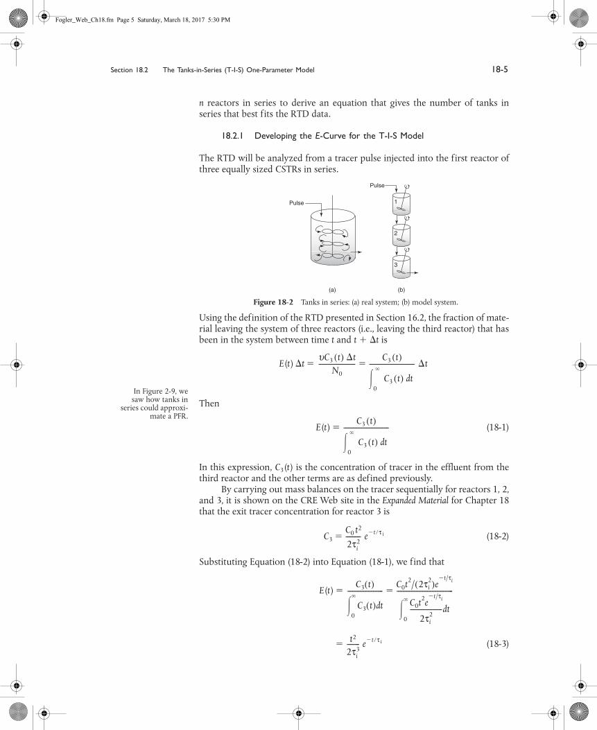
, in series that will give approximately the same RTD as the non-ideal reactor. Next, we will apply the reaction engineering algorithm developedin Chapters 1 through 5 to calculate conversion. We are first going to developthe RTD equation for three tanks in series (Figure 18-2) and then generalize to

Nonideal tubularreactors

t

Channeling

C(t)VS

VD

(a) (b) (c)

Dead zonesz = 0 z = L

vS

v

vv

Figure 18-1 (a) Real system; (b) outlet for a pulse input; (c) model system.

υb

υ0 υb υS

n = ?


Section 18.2 The Tanks-in-Series (T-I-S) One-Parameter Model

18-5

n

reactors in series to derive an equation that gives the number of tanks inseries that best fits the RTD data.

18.2.1 Developing the

E

-Curve for the T-I-S Model

The RTD will be analyzed from a tracer pulse injected into the first reactor ofthree equally sized CSTRs in series.

Using the definition of the RTD presented in Section 16.2, the fraction of mate-rial leaving the system of three reactors (i.e., leaving the third reactor) that hasbeen in the system between time

t

and

t

�

�

t

is

E

(

t

)

�

t

�

Then

E

(

t

)

�

(18-1)

In this expression,

C

3

(

t

) is the concentration of tracer in the effluent from thethird reactor and the other terms are as defined previously.

By carrying out mass balances on the tracer sequentially for reactors 1, 2,and 3, it is shown on the CRE Web site in the

Expanded Material

for Chapter 18that the exit tracer concentration for reactor 3 is

(18-2)

Substituting Equation (18-2) into Equation (18-1), we find that

E

(

t

)

�

�

(18-3)

In Figure 2-9, wesaw how tanks in

series could approxi-mate a PFR.

Pulse

Pulse

1

2

3

(b)(a)

Figure 18-2 Tanks in series: (a) real system; (b) model system.

υC3 t( ) �tN0

-----------------------C3 t( )

C 3 t ( ) t d 0

� �

---------------------------- � t �

C3 t( )

C 3 t ( ) t d 0

� �

----------------------------

C3C0 t2

2τi2

--------- e � t

τ

i

�

C3 t( )

C3 t( ) td0

�

�----------------------

C0t2/ 2τi2( )e

t/τi�

C0t2et/τi�

2τi2

--------------------dt0

�

�-----------------------------------�

t2

2τi3

-------- e � t

τ

i


18-6


Generalizing this method to a series of

n

CSTRs gives the RTD for

n

CSTRs in series,

E

(

t

):

(18-4)

Equation (18-4) will be a bit more useful if we put in the dimensionless form interms of

E

(

). Because the total reactor volume is

nV

i

, then

τ

i

�

τ

/

n

, where

τ

represents the total reactor volume divided by the flow rate, , we have

E

(

)

�

τ

E

(

t

) =

e

�

n

(18-5)

where

�

t

/

τ

�

Number of reactor volumes of fluid that have passed throughthe reactor after time

t

. Here, (

E

(

)

d

) is the fraction of material existing between dimensionlesstime

and time (

�

d

). Figure 18-3 illustrates the RTDs of various numbers of CSTRs in series in

a two-dimensional plot (a) and in a three-dimensional plot (b). As the numberbecomes very large, the behavior of the system approaches that of a plug-flowreactor.

We can determine the number of tanks in series by calculating thedimensionless variance from a tracer experiment.

�

(

�

1)

2

E

(

)

d

(18-6)

�

2

E

(

)

d

�

2

E

(

)

d

� E () d (18-7)

� 2 E () d � 1 (18-8)

RTD for equal-sizetanks in series E t( ) t n�1

n 1�( )!τin----------------------- e � t

τ

i �

υ

n n( )n�1

n 1�( )!-----------------------

1.4n=10

n=∞

n=4n=2

1.2

1

0.8

0.6

0.4

0.200 1 2

(a) (b)

3

510

15

0

E

12

34

0.5

1

1.5

n

Figure 18-3 Tanks-in-series response to a pulse tracer input for different numbers of tanks.

�2

�2 �2

τ2-----

0

� �

�

0

� �

0

� �

0

� �

�2

0

� �


Section 18.2 The Tanks-in-Series (T-I-S) One-Parameter Model

18-7

�

2

e

�

n

d

�

1

�

n

�

1

e

�

n

d

�

1 (18-9)

�

�

(18-10)

The number of tanks in series is

(18-11)

This expression represents the number of tanks necessary to model the realreactor as

n

ideal tanks in series. If the number of reactors,

n

, turns out to besmall, the reactor characteristics turn out to be those of a single CSTR orperhaps two CSTRs in series. At the other extreme, when

n

turns out to belarge, we recall from Chapter 2 that the reactor characteristics approachthose of a PFR.

18.2.2 Calculating Conversion for the T-I-S Model

If the reaction is first order, we can use Equation (5-15) to calculate theconversion

X

�

1

�

(5-15)

where

τ

i

�

It is acceptable (and usual) for the value of

n

calculated from Equation (18-11)to be a noninteger in Equation (5-15) to calculate the conversion. For reactionsother than first order, an integer number of reactors must be used and sequen-tial mole balances on each reactor must be carried out. If, for example,

n

= 2.53, then one could calculate the conversion for two tanks and also forthree tanks to bound the conversion. The conversion and effluent concentra-tions would be solved sequentially using the algorithm developed in Chapter5; that is, after solving for the effluent from the first tank, it would be used asthe input to the second tank and so on as shown on the CRE Web site forChapter 18 Expanded Materials .

0

� � n n( )n�1

n 1�

( )

!-----------------------

�2 nn

n 1�( )!------------------

0

� �

nn

n 1�( )!------------------ n 1

� ( ) !

n

n

�

2 ------------------ 1 �

As the number oftanks increases, thevariance decreases.

�2 1

n---

n 1�

2------- τ2

�2-----� �

11 τi k�( )n

-----------------------

Vυ0 n---------


18-8


18.2.3 Tanks-in-Series versus Segregation for a First-Order Reaction

We have already stated that the segregation and maximum mixedness modelsare equivalent for a first-order reaction. The proof of this statement was left asan exercise in Problem P17-3

B

. We can extend this equivalency for a first-orderreaction to the tanks-in-series (T-I-S) model

X T-I-S = X

seg = X mm (18-12)

The proof of Equation (18-12) is given in the

Expanded Materials

on theCRE Web site for Chapter 18 (

http://www.umich.edu/~elements/5e/18chap/expanded_ch18_example1.pdf

).

18.3 Dispersion One-Parameter Model

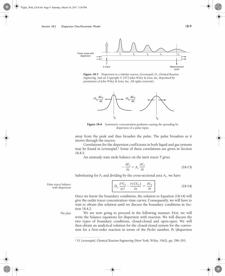
The dispersion model is also often used to describe nonideal tubular reactors.In this model, there is an axial dispersion of the material, which is governed byan analogy to Fick’s law of diffusion, superimposed on the flow as shown inFigure 18-4. So in addition to transport by bulk flow,

UA

c

C

, every componentin the mixture is transported through any cross section of the reactor at a rateequal to [–

D

a

A

c

(

dC

/

dz

)] resulting from molecular and convective diffusion. Byconvective diffusion (i.e., dispersion), we mean either Aris-Taylor dispersion inlaminar-flow reactors or turbulent diffusion resulting from turbulent eddies.Radial concentration profiles for plug flow (a) and a representative axial andradial profile for dispersive flow (b) are shown in Figure 18-4. Some moleculeswill diffuse forward ahead of the molar average velocity, while others will lagbehind.

To illustrate how dispersion affects the concentration profile in a tubularreactor, we consider the injection of a perfect tracer pulse. Figure 18-5 showshow dispersion causes the pulse to broaden as it moves down the reactor andbecomes less concentrated.

Recall Equation (14-14). The molar flow rate of tracer (

F

T

) by both con-vection and dispersion is

(14-14)

In this expression,

D

a

is the effective dispersion coefficient (m

2

/s) and

U

(m/s)is the superficial velocity. To better understand how the pulse broadens, werefer to the concentration peaks

t

2

and

t

3

in Figure 18-6. We see that there is aconcentration gradient on both sides of the peak causing molecules to diffuse

(a)

Plug Flow

(b)

Dispersion

Figure 18-4 Concentration profiles: (a) without and (b) with dispersion.

Tracer pulse withdispersion

FT Da �CT

�z--------� UCT� Ac�


Section 18.3 Dispersion One-Parameter Model

18-9

away from the peak and thus broaden the pulse. The pulse broadens as itmoves through the reactor.

Correlations for the dispersion coefficients in both liquid and gas systemsmay be found in Levenspiel.

2

Some of these correlations are given in Section18.4.5.

An unsteady state mole balance on the inert tracer

T

gives

(18-13)

Substituting for

F

T

and dividing by the cross-sectional area

A

c

, we have

(18-14)

Once we know the boundary conditions, the solution to Equation (18-14) willgive the outlet tracer concentration–time curves. Consequently, we will have towait to obtain this solution until we discuss the boundary conditions in Sec-tion 18.4.2.

We are now going to proceed in the following manner: First, we willwrite the balance equations for dispersion with reaction. We will discuss thetwo types of boundary conditions, closed-closed and open-open. We willthen obtain an analytical solution for the closed-closed system for the conver-sion for a first-order reaction in terms of the Peclet number,

Pe

(dispersion

2

O. Levenspiel,

Chemical Reaction Engineering

(New York: Wiley, 1962), pp. 290–293.

Measurementpoint

Tracer pulse withdispersion

t1 t2 t3 t4 t5

Figure 18-5 Dispersion in a tubular reactor. (Levenspiel, O., Chemical Reaction Engineering, 2nd ed. Copyright © 1972 John Wiley & Sons, Inc. Reprinted by permission of John Wiley & Sons, Inc. All rights reserved.)

dCTdz

dCTdz

t2 t 3

Figure 18-6 Symmetric concentration gradients causing the spreading by dispersion of a pulse input.

�FT

�z--------� Ac

� C

T �

t -------- �

Pulse tracer balancewith dispersion Da

�

2

C

T �

z

2 ----------

�

UC

T ( )

�

z ------------------ �

�

C

T �

t

-------- �

The plan


18-10


coefficient) and the Damköhler number. We then will discuss how the disper-sion coefficient can be obtained either from correlations in the literature

or

fromthe analysis of the RTD curve.

18.4 Flow, Reaction, and Dispersion

Now that we have an intuitive feel for how dispersion affects the transport ofmolecules in a tubular reactor, we shall consider two types of dispersion in atubular reactor,

laminar

and

turbulent

.

18.4.1 Balance Equations

In Chapter 14 we showed that the mole balance on reacting species A flow in atubular reactor was

(14-16)

Rearranging Equation (14-16) we obtain

(18-15)

This equation is a second-order ordinary differential equation. It is nonlinearwhen

r

A

is other than zero or first order.When the reaction rate

r

A

is first order,

r

A

= –

kC

A

, then Equation (18-16)

(18-16)

is amenable to an analytical solution. However, before obtaining a solution, weput our Equation (18-16) describing dispersion and reaction in dimensionlessform by letting

ψ

�

C

A

/

C

A0

and

�

z

/

L

(18-17)

The quantity

Da

1

appearing in Equation (18-17) is called the

Damköhlernumber

for a first-order conversion and physically represents the ratio

(18-18)

The other dimensionless term is the

Peclet number,

Pe

,

(18-19)

in which

l

is the characteristic length term. There are two different types ofPeclet numbers in common use. We can call

Pe

r

the

reactor

Peclet number; it

Dad2CA

dz2----------- U

dCA

dz--------� rA� 0�

Da

U------

d 2

C

A dz

2 -----------

dC

A dz

-------- � r

A

U ---- � 0 �

Da

U------

d 2

C

A dz

2 -----------

dC

A dz

-------- � kC

A

U -------- � 0 �Flow, reaction, and

dispersion

Da = Dispersioncoefficient

Da1 = Damköhlernumber

1Per------d2

�

d 2

-------- d�d ------� Da1 �� 0�

Damköhler numberfor a first-order

reaction

Da1Rate of consumption of A by reactionRate of transport of A by convection------------------------------------------------------------------------------------------- kτ� �

PerRate of transport by convection

Rate of transport by diffusion or dispersion-------------------------------------------------------------------------------------------------------- Ul

Da------� �


Section 18.4 Flow, Reaction, and Dispersion

18-11

uses the reactor length,

L

, for the characteristic length, so

Pe

r

�

UL

/

D

a

. It is

Pe

r

that appears in Equation (18-17). The reactor Peclet number,

Pe

r

, for mass dis-persion is often referred to as the Bodenstein number, Bo, in reacting systemsrather than the Peclet number. The other type of Peclet number can be calledthe

fluid

Peclet number,

Pe

f

; it uses the characteristic length that determines thefluid’s mechanical behavior. In a packed bed this length is the particle diameter

d

p

, and

Pe

f

�

Ud

p

/

�

D

a

. (The term

U

is the empty tube or superficial velocity.For packed beds we often wish to use the average interstitial velocity, and thus

U

/

�

is commonly used for the packed-bed velocity term.) In an empty tube,the fluid behavior is determined by the tube diameter

d

t

, and

Pe

f

�

Ud

t

/

D

a

. Thefluid Peclet number,

Pe

f

, is given in virtually all literature correlations relatingthe Peclet number to the Reynolds number because both are directly related tothe fluid mechanical behavior. It is, of course, very simple to convert

Pe

f

to

Pe

r

:Multiply by the ratio

L

/

d

p

or

L

/

d

t

. The reciprocal of

Pe

r

,

D

a

/

UL

, is sometimescalled the

vessel dispersion number

.

18.4.2 Boundary Conditions

There are two cases that we need to consider: boundary conditions for closedvessels and for open vessels. In the case of closed-closed vessels, we assume that thereis no dispersion or radial variation in concentration either upstream (closed) ordownstream (closed) of the reaction section; hence, this is a closed-closed ves-sel, as shown in Figure 18-7(a). In an open vessel, dispersion occurs bothupstream (open) and downstream (open) of the reaction section; hence, this isan open-open vessel as shown in Figure 18-7(b). These two cases are shown inFigure 18-7, where fluctuations in concentration due to dispersion are super-imposed on the plug-flow velocity profile. A closed-open vessel boundarycondition is one in which there is no dispersion in the entrance section butthere is dispersion in the reaction and exit sections.

18.4.2A Closed-Closed Vessel Boundary Condition

For a closed-closed vessel, we have plug flow (no dispersion) to the immediateleft of the entrance line (z = 0–) (closed) and to the immediate right of the exitz = L (z = L+) (closed). However, between z = 0+ and z = L–, we have dispersionand reaction. The corresponding entrance boundary condition is

At z = 0: FA(0–) = FA(0+)

For open tubesPer � 106,Pef � 104

For packed bedsPer � 103,Pef � 101

Figure 18-7 Types of boundary conditions.

Closed-closed vessel(a) (b) Open-open vessel


18-12 Models for Nonideal Reactors Chapter 18

Substituting for FA yields

UAc CA (0� ) � �Ac Da � UAc CA (0� )

Solving for the entering concentration CA(0–) = CA0

(18-20)

At the exit to the reaction section, the concentration is continuous, and thereis no gradient in tracer concentration.

At z � L: (18-21)

These two boundary conditions, Equations (18-20) and (18-21), f irststated by Danckwerts, have become known as the famous Danckwerts boundaryconditions.3 Bischoff has given a rigorous derivation by solving the differentialequations governing the dispersion of component A in the entrance and exitsections, and taking the limit as the dispersion coefficient, Da in the entranceand exit sections approaches zero.4 From the solutions, he obtained bound-ary conditions on the reaction section identical with those Danckwertsproposed.

The closed-closed concentration boundary condition at the entrance isshown schematically in Figure 18-8 on page 857. One should not be uncom-fortable with the discontinuity in concentration at z = 0 because if you recallfor an ideal CSTR, the concentration drops immediately on entering from CA0to CAexit. For the other boundary condition at the exit z = L, we see the concen-tration gradient, (dCA/dz), has gone to zero. At steady state, it can be shown thatthis Danckwerts boundary condition at z = L also applies to the open-open sys-tem at steady state.

18.4.2B Open-Open System

For an open-open system, there is continuity of flux at the boundaries at z = 0

FA(0–) = FA(0+)

(18-22)

3 P. V. Danckwerts, Chem. Eng. Sci., 2, 1 (1953).4 K. B. Bischoff, Chem. Eng. Sci., 16, 131 (1961).

FA→→

0� 0�

z � 0dCA

dz--------

⎝ ⎠⎜ ⎟⎛ ⎞

z�0�

Concentrationboundary

conditions at theentrance

CA0Da�

U-----------

dC

A dz

-------- ⎝ ⎠⎜ ⎟⎛ ⎞

z

�

0

�

C A 0 � ( ) ��

Concentrationboundary

conditions at the

CA L�( ) CA L�( )�

dCA

dz-------- 0�

DanckwertsBoundary

Conditions

Open-openboundary condition Da

�CA

�z---------⎠

⎞z 0�

�� UCA 0 �( )� Da

�CA

�z---------⎠

⎞z 0�

+� UCA 0+ ( )��



18-13

At

z

=

L,

we have continuity of concentration and

(18-23)

18.4.2C Back to the Solution for a Closed-Closed System

We now shall solve the dispersion reaction balance for a first-order reaction

(18-17)

For the closed-closed system, the Danckwerts boundary conditions in dimen-sionless form are

(18-24)

(18-25)

At the end of the reactor, where

λ

= 1, the solution to Equation (18-17) is

(18-26)

Figure 18-8

Schematic of Danckwerts boundary conditions: (a) entrance; (b) exit.

CA0

z = 0

CA(0+

0+−

−

−0 L+L

)

(z)

dCAdz

z =L

=0

CA CA(L ) (L+)

z = L

(b)(a)

CA0 =CA 0+( ) −Da dCA

dzU

⎞

⎠ ⎟

z = 0+

dCA

dz-------- 0�

1Per------d2

�

d 2

-------- d�d ------� Da1ψ� 0�

At 0 then 1= 1Per------d�

d ------⎠

⎞ 0�

+� ψ 0+( )��

At 1 then d�d ------ 0� �

Da1 = τkPer = UL/Da

Nomenclature note Da1 is the Damköhler number for a first-order reaction, τkDa is the dis-persion coeffi-cient in cm2/sPer = UL/Da

�LCAL

CA0-------- 1 X��

4q Per 2( )exp

1 q�( )2 Per q 2( )exp 1 q�( )2 exp ( Pe� r q/2)�---------------------------------------------------------------------------------------------------------------=

where q 1 4Da1/Per��

Prof. P. V. Danckwerts,Cambridge

University, U.K.



This solution was first obtained by Danckwerts and has been published inmany places (e.g., Levenspiel).5,6 With a slight rearrangement of Equation(18-26), we obtain the conversion as a function of Da1 and Per.

(18-27)

Outside the limited case of a first-order reaction, a numerical solution of theequation is required, and because this is a split-boundary-value problem, aniterative technique is needed.

To evaluate the exit concentration given by Equation (18-26) or the con-version given by (18-27), we need to know the Damköhler and Peclet numbers.The first-order reaction rate constant, k, and hence Da1 = τk, can be foundusing the techniques in Chapter 7. In the next section, we discuss methods todetermine Da by finding the Peclet number.

18.4.3 Finding Da and the Peclet Number

There are three ways we can use to find Da and hence Per1. Laminar flow with radial and axial molecular diffusion theory2. Correlations from the literature for pipes and packed beds3. Experimental tracer data

At first sight, simple models described by Equation (18-14) appear tohave the capability of accounting only for axial mixing effects. It will be shown,however, that this approach can compensate not only for problems caused byaxial mixing, but also for those caused by radial mixing and other nonflat velocity pro-files.7 These fluctuations in concentration can result from different flow veloci-ties and pathways and from molecular and turbulent diffusion.

18.4.4 Dispersion in a Tubular Reactor with Laminar Flow

In a laminar flow reactor, we know that the axial velocity varies in the radialdirection according to the well-known parabolic velocity profile:

u(r) = 2U

where U is the average velocity. For laminar flow, we saw that the RTD func-tion E(t) was given by

(16-47)

5 P. V. Danckwerts, Chem. Eng. Sci., 2, 1 (1953).6 Levenspiel, Chemical Reaction Engineering, 3rd ed. (New York: Wiley, 1999).7 R. Aris, Proc. R. Soc. (London), A235, 67 (1956).

X 14q Per 2( )exp

1 q�( )2 Per q 2( )exp 1 q�( )2 exp ( Pe� r q/2)�---------------------------------------------------------------------------------------------------------------��

Three ways tofind Da

1 rR---⎝ ⎠

⎛ ⎞2�

E t( )0 for t τ

2 --- τ L

U ---- � ⎝ ⎠

⎛ ⎞ �

τ

2

2

t

3

------ for t τ 2

--- � ⎩⎪⎪⎨⎪⎪⎧

�



18-15

In arriving at this distribution

E

(

t

), it was assumed that there was no transfer ofmolecules in the radial direction between streamlines. Consequently, with theaid of Equation (16-47), we know that the molecules on the center streamline(

r

= 0) exited the reactor at a time

t

=

τ

/2, and molecules traveling on thestreamline at

r

= 3

R

/4 exited the reactor at time

The question now arises: What would happen if some of the moleculestraveling on the streamline at

r

=

3R/4

jumped (i.e., diffused) onto the stream-line at

r

=

0

? The answer is that they would exit sooner than if they had stayedon the streamline at

r

=

3R/4

. Analogously, if some of the molecules from thefaster streamline at

r

=

0

jumped (i.e., diffused) onto the streamline at

r

=

3R/4

,they would take a longer time to exit (Figure 18-9). In addition to the moleculesdiffusing between streamlines, they can also move forward or backward rela-tive to the average fluid velocity by molecular diffusion (Fick’s law). With bothaxial and radial diffusion occurring, the question arises as to what will be thedistribution of residence times when molecules are transported between andalong streamlines by diffusion. To answer this question, we will derive anequation for the axial dispersion coefficient,

D

a

, that accounts for the axial andradial diffusion mechanisms. In deriving

D

a

, which is often referred to as the

Aris–Taylor dispersion coefficient

, we closely follow the development given byBrenner and Edwards.

8

The convective–diffusion equation for solute (e.g., tracer) transport inboth the axial and radial direction can be obtained by combining Equation(14-3) with the diffusion equation (cf. Equation (14-11)) applied to the tracerconcentration,

c

, and transformed to radial coordinates

(18-28)

8

H. Brenner and D. A. Edwards,

Macrotransport Processes

(Boston: Butterworth-Heinemann, 1993).

t Lu-- L

2U 1 r R( )2�[ ]

------------------------------------ τ2 1 3 4( )2

�[ ]--------------------------------� � �

87--- τ�=

Molecules diffusingbetween stream-

lines and back andforth along a

Figure 18-9 Radial diffusion in laminar flow.

�c�t----- u r( ) � c

�

z ----- � � D AB 1

r --- � r

� c

� r

( )[ ]

� r ----------------------------

�

2 c

�

z

2 ------- �

⎩ ⎭⎨ ⎬⎧ ⎫


18-16


where

c

is the solute concentration at a particular

r

,

z

, and

t

, and

D

AB

is themolecular diffusion coefficient of species A in B.

We are going to change the variable in the axial direction

z

to , whichcorresponds to an observer moving with the fluid

z

*

=

z

–

Ut

(18-29)

A value of

�

0 corresponds to an observer moving with the average velocityof the fluid,

U

. Using the chain rule, we obtain

(18-30)

Because we want to know the concentrations and conversions at the exit to thereactor, we are really only interested in the average axial concentration, ,which is given by

(

z

,

t

)

�

c

(

r

,

z

,

t

)2

�

r dr

(18-31)

Consequently, we are going to solve Equation (18-30) for the solution concentra-tion as a function of r and then substitute the solution

c (r, z, t)

into Equation(18-31) to find (

z

,

t

). All the intermediate steps are given on the CRE Web sitein the

Professional Reference Shelf

, and the partial differential equation describing thevariation of the average axial concentration with time and distance is

(18-32)

where is the Aris-Taylor dispersion coefficient

(18-33)

That is, for laminar flow in a pipe

Figure 18-10 shows the dispersion coefficient in terms of the ratio/

U

(2

R

)

�

/

Ud

t

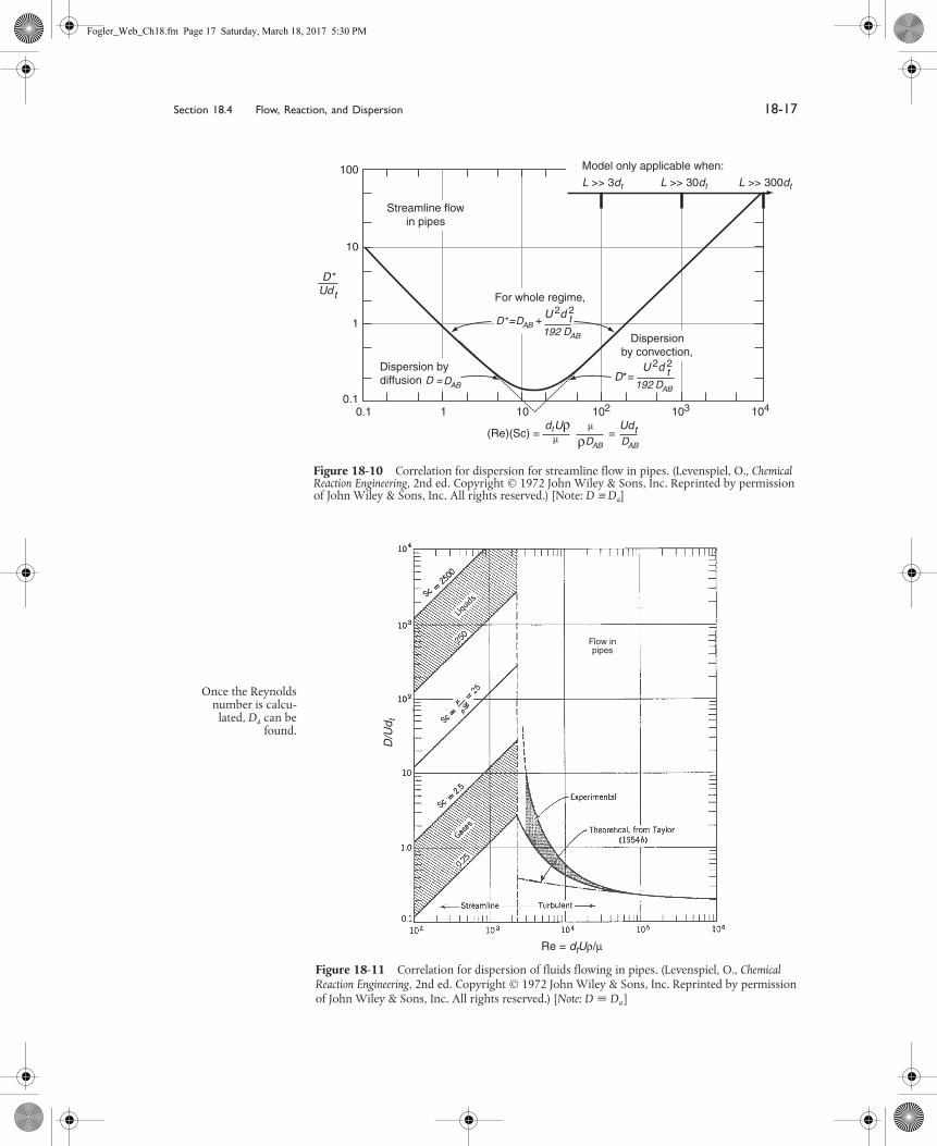
as a function of the product of the Reynolds (Re) andSchmidt (Sc) numbers.

18.4.5 Correlations for

D

a

We will use correlations from the literature to determine the dispersion coeffi-cient

D

a

for flow in cylindrical tubes (pipes) and for flow in packed beds.

18.4.5A Dispersion for Laminar and Turbulent Flow in Pipes

An estimate of the dispersion coefficient,

D

a

, can be determined from Figure18-11. Here,

d

t

is the tube diameter and

Sc

is the Schmidt number discussed inChapter 14. The flow is laminar (streamline) below 2,100, and we see the ratio

z�

z�

�c�t-----

⎝ ⎠⎜ ⎟⎛ ⎞

z�

u r( ) U�[ ] � c �

z

� ------- � D AB 1

r --- �

� r ---- r � c

�

r -----

⎝ ⎠⎜ ⎟⎛ ⎞

�

2 c

�

z

�

2 --------- ��

C

C 1�R2---------

0

R �

C

�C�t------ U � C

�

z � ------- � D

� �

2 C

�

z �

2 --------- �

D�

Aris-Taylordispersioncoefficient

D� DABU2R2

48DAB---------------��

Da D��

D�

D� D�



18-17

100

10

1

0.10.1 1 10 102 103 104

D*Udt

Streamline flowin pipes

Dispersionby convection,

U 2d 2D* = t

For whole regime,

U 2d 2t

(Re)(Sc) = = UdU t

DD* =192

192D =

ABDAB

DAB

DABDAB

DAB

Model only applicable when:

L >> 3dt L >> 30dt L >> 300dt

dt

Dispersion bydiffusion

Figure 18-10 Correlation for dispersion for streamline flow in pipes. (Levenspiel, O., Chemical Reaction Engineering, 2nd ed. Copyright © 1972 John Wiley & Sons, Inc. Reprinted by permission of John Wiley & Sons, Inc. All rights reserved.) [Note: D ≡ Da]

D/U

d t

Re = dtUρ/μ

Flow inpipes

Figure 18-11

Correlation for dispersion of fluids flowing in pipes. (Levenspiel, O.,


, 2nd ed. Copyright © 1972 John Wiley & Sons, Inc. Reprinted by permission of John Wiley & Sons, Inc. All rights reserved.) [

Note

:

D

�

D

a

]

Once the Reynoldsnumber is calcu-

lated, Da can befound.


18-18


(

D

a

/Ud

t

) increases with increasing Schmidt and Reynolds numbers. Between Rey-nolds numbers of 2,100 and 30,000, one can put bounds on

D

a

by calculating themaximum and minimum values at the top and bottom of the shaded regions.

18.4.5B Dispersion in Packed Beds

For the case of gas–solid and liquid–solid catalytic reactions that take place inpacked-bed reactors, the dispersion coefficient,

D

a

, can be estimated by usingFigure 18-12. Here,

d

p

is the particle diameter and

ε

is the porosity.

18.4.6 Experimental Determination of

D

a

The dispersion coefficient can be determined from a pulse tracer experiment.Here, we will use

t

m

and

�

2

to solve for the dispersion coefficient

D

a

and thenthe Peclet number,

Pe

r

. Here the effluent concentration of the reactor is mea-sured as a function of time. From the effluent concentration data, the meanresidence time,

t

m

, and variance,

�

2

, are calculated, and these values are thenused to determine

D

a

. To show how this is accomplished, we will write theunsteady state mass balance on the tracer flowing in a tubular reactor

(18-13)

in dimensionless form, discuss the different types of boundary conditions atthe reactor entrance and exit, solve for the exit concentration as a function ofdimensionless time (

�

t

/

τ

), and then relate

D

a

,

�

2

, and

τ.

18.4.6A The Unsteady-State Tracer Balance

The first step is to put Equation (18-13) in dimensionless form to arrive at thedimensionless group(s) that characterize the process. Let

ψ � , � , and �

D/U

d pε

Re = dpUρ/μ

Figure 18-12 Experimental findings on dispersion of fluids flowing with mean axial velocity u in packed beds. (Levenspiel. O., Chemical Reaction Engineering, 2nd ed. Copyright © 1972 John Wiley & Sons, Inc. Reprinted by permission of John Wiley & Sons, Inc. All rights reserved.) [Note: D � Da ]

Da�

2CT

�z2----------

� UCT( )�z

-----------------��CT

�t--------�

CT

CT0------- z

L-- tU

L-----


Section 18.4 Flow, Reaction, and Dispersion 18-19

For a pulse input, CT0 is defined as the mass of tracer injected, M, divided by thevessel volume, V. Then

(18-34)

The initial condition is

At t = 0, z > 0, CT(0+,0) = 0, �(0+)� 0 (18-35)

The mass of tracer injected, M, is

M = UAc (0–, t) dt

18.4.6B Solution for a Closed-Closed System

In dimensionless form, the Danckwerts boundary conditions are

At λ = 0: (18-36)

At λ = 1: (18-37)

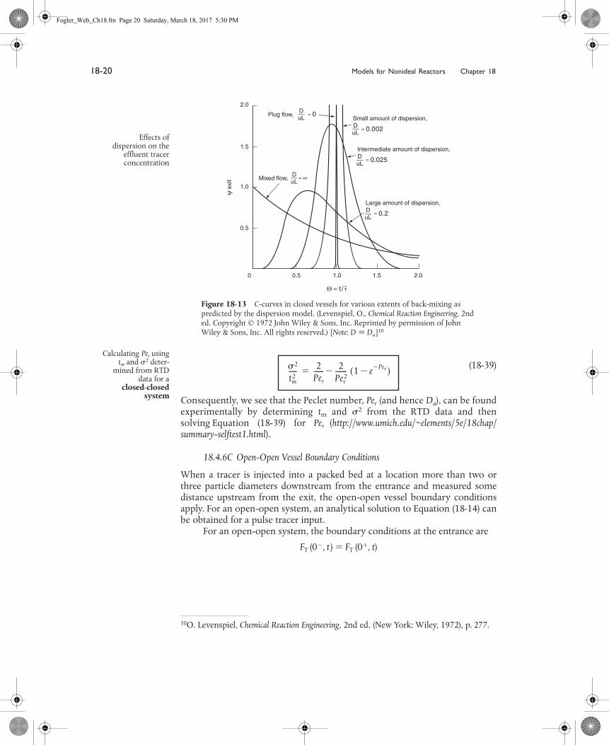
Equation (18-34) has been solved numerically for a pulse injection, and theresulting dimensionless effluent tracer concentration, �exit, is shown as a func-tion of the dimensionless time Θ in Figure 18-13 for various Peclet numbers.Although analytical solutions for � can be found, the result is an infinite series.The corresponding equations for the mean residence time, tm , and the variance,�2, are9

(18-38)

and

(t � τ)2 E (t ) dt

which can be used with the solution to Equation (18-34) to obtain

9 See K. Bischoff and O. Levenspiel, Adv. Chem. Eng., 4, 95 (1963).

1Per------ �

2

�

�

2 --------- ��

� ------ �

��

------- �

Initial condition

CT0

�

�

1Per------�

�� ------⎝ ⎠

⎛ ⎞ 0�

+� 0+( )�

CT 0 � t,( )CT0

--------------------- 1� �

�� ------ 0�

0 L0+ L+

tm t�

�2

tm2

----- 1t2----

0

� �

�


18-20


(18-39)

Consequently, we see that the Peclet number,

Pe

r

(and hence

D

a

), can be foundexperimentally by determining

t

m

and

�

2

from the RTD data and thensolving Equation (18-39) for

Pe

r

(

http://www.umich.edu/~elements/5e/18chap/summary-selftest1.html

).

18.4.6C Open-Open Vessel Boundary Conditions

When a tracer is injected into a packed bed at a location more than two orthree particle diameters downstream from the entrance and measured somedistance upstream from the exit, the open-open vessel boundary conditionsapply. For an open-open system, an analytical solution to Equation (18-14) canbe obtained for a pulse tracer input.

For an open-open system, the boundary conditions at the entrance are

F

T

(0

�

,

t

)

�

F

T

(0

�

,

t

)

10

O. Levenspiel,


, 2nd ed. (New York: Wiley, 1972), p. 277.

2.0

1.5

1.0

0.5

0 0.5 1.0 1.5 2.0

Mixed flow, DuL

=

Plug flow, DuL

= 0

DuL

= 0.002

Small amount of dispersion,

DuL

= 0.025

Intermediate amount of dispersion,

DuL

= 0.2

Large amount of dispersion,

τ

∞

Figure 18-13 C-curves in closed vessels for various extents of back-mixing as predicted by the dispersion model. (Levenspiel, O., Chemical Reaction Engineering, 2nd ed. Copyright © 1972 John Wiley & Sons, Inc. Reprinted by permission of John Wiley & Sons, Inc. All rights reserved.) [Note: D � Da ]10

Calculating Per usingtm and �2 deter-

mined from RTDdata for a

closed-closedsystem

�2

tm2

----- 2Per------ 2

Per2

------- 1 e Pe

r

�

� ( ) ��

Effects ofdispersion on the

effluent tracerconcentration



18-21

Then, for the case when the dispersion coefficient is the same in the entranceand reaction sections

(18-40)

Because there are no discontinuities across the boundary at

z

= 0

(18-41)

At the exit

(18-42)

(18-43)

There are a number of perturbations of these boundary conditions that can beapplied. The dispersion coefficient can take on different values in each of thethree regions (

z

< 0, 0 ≤

z

≤

L

, and

z

>

L

), and the tracer can also be injected atsome point

z

1

rather than at the boundary,

z

= 0. These cases and others can befound in the supplementary readings cited at the end of the chapter. We shallconsider the case when there is no variation in the dispersion coefficient for all

z

and an impulse of tracer is injected at

z

= 0 at

t

= 0.

For long tubes ( Pe r > 100) in which the concentration gradient at ± ∞ willbe zero, the solution to Equation (18-34) at the exit is

11

(18-44)

The mean residence time for an open-open system is

(18-45)

where

τ

is based on the volume between z = 0 and z = L (i.e., reactor volumemeasured with a yardstick). We note that the mean residence time for an opensystem is greater than that for a closed system. The reason is that the moleculescan diffuse back into the reactor after they diffuse out at the entrance. The vari-ance for an open-open system is

(18-46)

11

W. Jost,

Diffusion in Solids, Liquids and Gases

(New York: Academic Press, 1960), pp. 17, 47.

Open at theentrance

Da�CT

�z--------⎝ ⎠

⎛ ⎞z 0

��

� UCT 0 � t,( )� Da�CT

�z--------⎝ ⎠

⎛ ⎞z 0

+�

� UCT 0+ t,( )��

CT 0 � t,( ) CT 0+ t,( )�

Open at the exit Da�CT

�z--------⎝ ⎠

⎛ ⎞z L

��

� UCT L � t,( )� Da�CT

�z--------⎝ ⎠

⎛ ⎞z L

+�

� UCT L+ t,( )��

CT L � t,( ) CT L+ t,( )�

Valid for Per > 100� 1 ,( ) CT L t,( )

CT0---------------- 1

2 � Per------------------------- exp 1 �( )2

�4 Pe r

-------------------------� �

Calculate τ for anopen-open system

tm 1 2Per------�⎝ ⎠

⎛ ⎞τ�

Calculate Per for anopen–open system

�2

τ2----- 2

Per------ 8

Per2

-------��



We now consider two cases for which we can use Equations (18-39) and (18-46)to determine the system parameters:

Case 1. The space time τ is known. That is, V and υ0 are measured inde-pendently. Here, we can determine the Peclet number by deter-mining tm and �2 from the concentration–time data and thenuse Equation (18-46) to calculate Per. We can also calculate tmand then use Equation (18-45) as a check, but this is usually lessaccurate.

Case 2. The space time τ is unknown. This situation arises when thereare dead or stagnant pockets that exist in the reactor alongwith the dispersion effects. To analyze this situation, we firstcalculate mean residence time, tm, and the variance, �2, fromthe data as in case 1. Then, we use Equation (18-45) to elimi-nate τ2 from Equation (18-46) to arrive at

(18-47)

We now can solve for the Peclet number in terms of our exper-imentally determined variables �2 and . Knowing Per, we cansolve Equation (18-45) for τ, and hence V. The dead volume isthe difference between the measured volume (i.e., with a yard-stick) and the effective volume calculated from the RTD.

Example 18–1 Conversion Using Dispersion and Tanks-in-Series Models

The first-order reaction

A B

is carried out in a 10-cm-diameter tubular reactor 6.36 m in length. The specificreaction rate is 0.25 min�1. The results of a tracer test carried out on this reactor areshown in Table E18-1.1.

Calculate the conversion using (a) the closed vessel dispersion model, (b) PFR,(c) the tanks-in-series model, and (d) a single CSTR.

Solution

(a) We will use Equation (18-27) to calculate the conversion

(18-27)

where Da1 � τk, and Per � UL/Da .

TABLE E18-1.1 EFFLUENT TRACER CONCENTRATION AS A FUNCTION OF TIME

t (min) 0 1 2 3 4 5 6 7 8 9 10 12 14

C (mg/L) 0 1 5 8 10 8 6 4 3 2.2 1.5 0.6 0

�2

tm2

-----2Per 8�

Pe r2 4Per 4� �

----------------------------------�

Finding the effectivereactor volume

tm2

⎯⎯→

X 14q Pe r 2 ( ) exp

1

q

�

( )

2 Pe r q 2 ( ) 1 q � ( ) 2 P � e r q 2 ( ) exp � exp-----------------------------------------------------------------------------------------------------------------

��

q 1 4Da1 Per��



18-23

(1) Parameter evaluation using the RTD data to evaluate

Pe

r

:

We can calculate

Pe

r

from Equation (18-39)

(18-39)

However, we must find

τ

2

and

�

2

from the tracer concentration data first.

We note that this is the same data set used in Examples 16-1 and 16-2

T

ABLE

E18-1.2 P

OLYMATH

P

ROGRAM

AND

R

ESULTS

TO

C

ALCULATE

THE

M

EAN

R

ESIDENCE

T

IME

, t

m

,

AND

THE

VARIANCE

�

2

where we found

t

m

�

5.15 minutes

and

�

2

�

6.1 minutes

2

We will use these values in Equation 18-39 to calculate

Pe

r

.Dispersion in a closed vessel is represented by

(18-39)

Solving for

Pe

r

either by trial and error or using Polymath, we obtain

Pe

r

�

7.5 (E18-1.3)

(2) Next, we calculate

Da

1

and

q

:

Da

1

�

τ

k

�

(5.15 min)(0.25 min

�

1

)

�

1.29 (E18-1.4)

Using the equations for q and X gives

(E18-1.5)

�2

t2----- 2

Per------ 2

Per2

------- 1 e Per

� � ( ) ��

First calculate tm and�2 from RTD data.

t tE t ( ) td

0

� �

V υ

---

� �

�

2 t t � ( ) 2 E t ( ) td

0

� �

�

Here again,spreadsheets can beused to calculate τ2

and �2.

Calculated values of DEQ variablesVariable Initial value Final value

1 Area 51. 51.2 C 0.0038746 0.01480433 C1 0.0038746 -387.2664 C2 -33.43818 0.01480435 E 7.597E-05 0.00029036 Sigma2 0 6.2124737 t 0 14.8 tmf 5.1 5.1

Differential equations

1 d(Sigma2)/d(t) = (t-tmf)^2*E

Explicit equations

1 C1 = 0.0038746 + 0.2739782*t + 1.574621*t^2 - 0.2550041*t^32 Area = 513 C2 = -33.43818 + 37.18972*t - 11.58838*t^2 + 1.695303*t^3 -

0.1298667*t^4 + 0.005028*t^5 - 7.743*10^-5*t^64 C = If(t<=4 and t>=0) then C1 else if(t>4 and t<=14) then C2 else 05 E = C/Area6 tmf = 5.1

POLYMATH Report

Ordinary Differential Equations

Don’t fall asleep.These are

calculations weneed to know how

to carry out.

Calculate Per fromtm and �2.

�2

t2----- 2

Per2

------- Pe r 1 � e Pe

r

�

� ( ) �

6.15.15

( )

2

----------------

0.23 2

Pe

r

2

------- Pe r 1 � e Per

� � ( ) � � �

Next, calculateDa1 , q, and X.

q 14Da1

Per-------------� 1 4 1.29( )

7.5-----------------� 1.30� � �

(E18-1.1)

(E18-1.2)


18-24


Then

(E18-1.6)

(3) Finally, we calculate the conversion:

Substitution into Equation (18-27) yields

When dispersion effects are present in this tubular reactor, 68% conversionis achieved.

(b)

If the reactor were operating ideally as a plug-flow reactor, the conversionwould be

X

�

1

�

e

�

τ

k

�

1

�

e

�

Da1

�

1

�

e

�

1.29

�

0.725 (E18-1.7)

That is, 72.5% conversion would be achieved in an ideal plug-flow reactor.(c)

Conversion using the tanks-in-series model: We recall Equation (18-11) tocalculate the number of tanks in series:

(E18-1.8)

To calculate the conversion for the T-I-S model, we recall Equation (5-15). For afirst-order reaction for

n

tanks in series, the conversion is

(E18-1.9)

(d)

For a single CSTR

(E18-1.10)

So, 56.3% conversion would be achieved in a single ideal tank.Summary:

In this example, correction for finite dispersion, whether by a dispersion model or atanks-in-series model, is significant when compared with a PFR.

Analysis:

This example is a very important and comprehensive one. We showedhow to calculate the conversion by (1) choosing a model, (2) using the RTD to eval-uate the model parameters, and (3) substituting the reaction-rate parameters in thechosen model. As expected, the dispersion and T-I-S model gave essentially thesame result and this result fell between the limits predicted by an ideal PFR and anideal CSTR.

Per q2

--------- 7.5( ) 1.3( )2

----------------------- 4.87� �

Dispersion modelX 1 4 1.30( ) e 7.5 2( )

2.3( )2 4.87 ( ) 0.3 � ( ) 2 4.87 � ( ) exp � exp -------------------------------------------------------------------------------------------------

��

X

0.68 68% conversion for the dispersion model

�

PFR

Tanks-in-seriesmodel

n t2

�2----- 5.15( )2

6.1---------------- 4.35� � �

X 1 11 ti k�( )n

----------------------� 1 11 t n( ) k�[ ]n

--------------------------------� 1 11 1.29 4.35�( )4.35

--------------------------------------------��

X 67.7% for the tanks-in-series model�

CSTR X tk1 tk�-------------- 1.29

2.29---------- 0.563� � �

Summary

PFR: X 72.5%�

Dispersion: X 68.0%�

Tanks in series: X 67.7%�

Single CSTR: X 56.3%�


Section 18.5 Tanks-in-Series Model versus Dispersion Model

18-25

18.5 Tanks-in-Series Model versus Dispersion Model

We have seen that we can apply both of these one-parameter models to tubularreactors using the variance of the RTD. For first-order reactions, the two mod-els can be applied with equal ease. However, the tanks-in-series model is math-ematically easier to use to obtain the effluent concentration and conversion forreaction orders other than one, and for multiple reactions. However, we needto ask what would be the accuracy of using the tanks-in-series model over thedispersion model. These two models are equivalent when the Peclet–Boden-stein number is related to the number of tanks in series,

n

, by the equation

12

Bo

= 2(

n

– 1) (18-48)

or

(18-49)

where

Bo

=

UL

/

D

a

(18-50)

where

U

is the superficial velocity,

L

the reactor length, and

D

a

the dispersioncoefficient.

For the conditions in Example 18-1, we see that the number of tanks cal-culated from the Bodenstein number, Bo (i.e., Per), Equation (18-49), is 4.75,which is very close to the value of 4.35 calculated from Equation (18-11). Con-sequently, for reactions other than first order, one would solve successively forthe exit concentration and conversion from each tank in series for both a bat-tery of four tanks in series and for five tanks in series in order to bound theexpected values.

In addition to the one-parameter models of tanks-in-series and disper-sion, many other one-parameter models exist when a combination of idealreactors is used to model the real reactor shown in Section 18.7 for reactorswith bypassing and dead volume. Another example of a one-parameter modelwould be to model the real reactor as a PFR and a CSTR in series with the oneparameter being the fraction of the total volume that behaves as a CSTR. Wecan dream up many other situations that would alter the behavior of idealreactors in a way that adequately describes a real reactor. However, it may bethat one parameter is not sufficient to yield an adequate comparison betweentheory and practice. We explore these situations with combinations of idealreactors in the section on two-parameter models.

The reaction-rate parameters are usually known (e.g., Da), but the Pecletnumber is usually not known because it depends on the flow and the vessel.Consequently, we need to find Per using one of the three techniques discussedearlier in the chapter.

12K. Elgeti, Chem. Eng. Sci., 51, 5077 (1996).

Equivalencybetween models oftanks-in-series and

dispersion n Bo2------ 1��



18.6 Numerical Solutions to Flows with Dispersion and Reaction

We now consider dispersion and reaction in a tubular reactor. We first writeour mole balance on species A in cylindrical coordinates by recalling Equation(18-28) and including the rate of formation of A, rA. At steady state we obtain

(18-51)

Analytical solutions to dispersion with reaction can only be obtained for iso-thermal zero- and first-order reactions. We are now going to use COMSOL tosolve the flow with reaction and dispersion with reaction.

We are going to compare two solutions: one which uses the Aris–Taylorapproach and one in which we numerically solve for both the axial and radialconcentration using COMSOL. These solutions are on the CRE Web site.

Case A. Aris-Taylor Analysis for Laminar Flow

For the case of an nth-order reaction, Equation (18-15) is

(18-52)

where is the average concentration from r = 0 to r = R, i.e.,

If we use the Aris-Taylor analysis, we can use Equation (18-15) with a caveatthat and λ = z/L we obtain

(18-53)

where

For the closed-closed boundary conditions we have

(18-54)

DAB1r---

� r�CA

�r---------⎝ ⎠

⎛ ⎞

�r-------------------

�2CA

�z2-----------� u r( )

�CA

�z---------� rA� 0�

Da

U------d2

CA

dz2----------- dCA

dz--------�

kCAn

U--------� 0�

CA

CA

CA r z,( ) rd0

r�R

---------------------------�

� CA CA0�

1Per------d2

�

d 2

--------- d�d ------� Dan�

n� 0�

PerULDa------- and Dan tkCA0

n 1��

At 0:�1

Per------d�

d ------

0�+

� � 0+( )� 1�

Danckwerts bound-ary conditions At 1:� d�

d ------ 0�


Section 18.7 Two-Parameter Models—Modeling Real Reactors with Combinations of Ideal Reactors 18-27

For the open-open boundary conditions we have

(18-55)

Equation (18-53) is a nonlinear second-order ODE that is solved on the COMSOLon the CRE Web site.

Case B. Full Numerical Solution

To obtain profiles, CA(r,z), we now solve Equation (18-51)

(18-51)

First, we will put the equations in dimensionless form by letting ,λ = z/L, and φ = r/R. Following our earlier transformation of variables, Equation(18-52) becomes

(18-56)

Equation (18-56) gives the dimensionless concentration profiles for dispersionand reaction in a laminar-flow reactor. The Expanded Material on the CRE Website gives an example, Web Example 18-2, where COMSOL is used to find theconcentration profile.

18.7 Two-Parameter Models—Modeling Real Reactors with Combinations of Ideal Reactors

We now will see how a real reactor might be modeled by different combina-tions of ideal reactors. Here, an almost unlimited number of combinations thatcould be made. However, if we limit the number of adjustable parameters totwo (e.g., bypass flow rate, υb, and dead volume, VD), the situation becomesmuch more tractable. After reviewing the steps in Table 18-1, choose a modeland determine if it is reasonable by qualitatively comparing it with the RTDand, if it is, determine the model parameters. Usually, the simplest means ofobtaining the necessary data is some form of a tracer test. These tests havebeen described in Chapters 16 and 17, together with their uses in determiningthe RTD of a reactor system. Tracer tests can be used to determine the RTD,which can then be used in a similar manner to determine the suitability of themodel and the value of its parameters.

At 0:� � 0 �( ) 1Per------d�

d ------

0� �

� � 0+( ) 1Per------d�

d ------

0�+

��

At 1:� d�d ------ 0�

DAB1r---

� r�CA

�r---------⎝ ⎠

⎛ ⎞

�r-------------------

�2CA

�z2-----------� u r( )

�CA

�z---------� rA� 0�

� CA CA0�

LR---⎝ ⎠

⎛ ⎞ 1Per------ 1

�----

� ��-------⎝ ⎠

⎛ ⎞

��------------------- 1

Per------d2

�

d 2

-------- 2 1 �2

�( )d�d ------� Dan�

n�� 0�

Creativity andengineering

judgment arenecessary for model

formulation.

A tracerexperiment is used

to evaluate themodel parameters.



In determining the suitability of a particular reactor model and theparameter values from tracer tests, it may not be necessary to calculate theRTD function E (t ). The model parameters (e.g., VD) may be acquired directlyfrom measurements of effluent concentration in a tracer test. The theoreticalprediction of the particular tracer test in the chosen model system is comparedwith the tracer measurements from the real reactor. The parameters in themodel are chosen so as to obtain the closest possible agreement between themodel and experiment. If the agreement is then sufficiently close, the model isdeemed reasonable. If not, another model must be chosen.

The quality of the agreement necessary to fulfill the criterion “suffi-ciently close” again depends on creativity in developing the model and on engi-neering judgment. The most extreme demands are that the maximum error inthe prediction not exceed the estimated error in the tracer test, and that therebe no observable trends with time in the difference between prediction (themodel) and observation (the real reactor). To illustrate how the modeling is car-ried out, we will now consider two different models for a CSTR.

18.7.1 Real CSTR Modeled Using Bypassing and Dead Space

A real CSTR is believed to be modeled as a combination of an ideal CSTR witha well-mixed volume Vs , a dead zone of volume Vd , and a bypass with a volu-metric flow rate (Figure 18-14). We have used a tracer experiment to evalu-ate the parameters of the model Vs and . Because the total volume andvolumetric flow rate are known, once Vs and are found, and Vd canreadily be calculated.

18.7.1A Solving the Model System for CA and X

We shall calculate the conversion for this model for the first-order reaction

A B

The bypass stream and effluent stream from the reaction volume are mixed atthe junction point 2. From a balance on species A around this point

(18-57)

The model system

υbυs

υs υb

Figure 18-14 (a) Real system; (b) model system.

⎯⎯→

The Duct Tape Councilof Jofostan would like

to point out thenew wrinkle: The

Junction Balance.

In[ ] Out[ ]�

CA0υb CAsυs�[ ] CA υb υs�( )[ ]�


Section 18.7 Two-Parameter Models—Modeling Real Reactors with Combinations of Ideal Reactors

We can solve for the concentration of A leaving the reactor

Let

�

�

V

s

/

V

and

�

�

. Then

C

A

�

�

C

A0

�

(1

�

�

)

C

A

s

(18-58)

For a first-order reaction, a mole balance on

V

s

gives

C

A0

�

C

A

s

�

kC

A

s

V

s

�

0 (18-59)

or, in terms of

�

and

�

(18-60)

Substituting Equation (18-60) into (18-58) gives the effluent concentration ofspecies A:

(18-61)

We have used the ideal reactor system shown in Figure 18-14 to predictthe conversion in the real reactor. The model has two parameters,

�

and

�

. Theparameter

α

is the dead zone volume fraction and parameter

β

is the fractionof the volumetric flow rate that bypasses the reaction zone. If these parametersare known, we can readily predict the conversion. In the following section, weshall see how we can use tracer experiments and RTD data to evaluate themodel parameters.

18.7.1B Using a Tracer to Determine the Model Parameters in a CSTR-with-Dead-Space-and-Bypass Model

In Section 18.7.1A, we used the system shown in Figure 18-15, with bypassflow rate, , and dead volume,

V

d

, to model our real reactor system. We shallinject our tracer,

T

, as a positive-step input. The unsteady-state balance on thenonreacting tracer,

T

, in the well-mixed reactor volume,

V

s

, isIn – out = accumulation

(18-62)

The conditions for the positive-step input are

A balance around junction point 2 gives

(18-63)

CAυbCA0 CAs υs�

υb υs�---------------------------------

υbCA0 CAs υs�

υ0---------------------------------� �

υb υ0

Mole balance onCSTR υs υs

CAsCA0 1 ��( ) υ0

1 ��( ) υ0 �Vk�----------------------------------------�

Conversion as afunction of model

parameters

CA

CA0-------- 1 X� �

1 ��( )2

1 ��( ) �tk�---------------------------------��

υb

Tracer balance forstep input υsCT0 � υ s C Ts �

dN

Ts dt ---------- V s

dC

Ts dt --------- �

Model system

At t 0�

At t 0�

CT 0�

CT CT0�

The junctionbalance CT

υbCT0 CTs υs�

υ0--------------------------------�


18-30


As before

Integrating Equation (18-62) and substituting in terms of

�

and

�

gives

(18-64)

Combining Equations (18-63) and (18-64), the effluent tracer concentration is

(18-65)

We now need to rearrange this equation to extract the model parameters,

α

and

β

, either by regression (Polymath/MATLAB/Excel) or from the proper plotof the effluent tracer concentration as a function of time. Rearranging yields

(18-66)

Consequently, we plot ln[

C

T

0

/ (

C

T

0

�

C

T

)] as a function of

t

. If our modelis correct, a straight line should result with a slope of (1

�

�

) /

τ

�

and an inter-

cept of ln[1/(1 � � )].

Example 18–2 CSTR with Dead Space and Bypass

The elementary reaction

A

�

B C

�

D

is to be carried out in the CSTR shown schematically in Figure 18-15. There is bothbypassing and a stagnant region in this reactor. The tracer output for this reactor isshown in Table E18-2.1. The measured reactor volume is 1.0 m

3

and the flow rate tothe reactor is 0.1 m

3

/min. The reaction-rate constant is 0.28 m

3

/kmol

�

min. The feed

CT0

CT0

CT

CTS

1

2

v0

v0

v0v

v0 v v

v

Figure 18-15 Model system: CSTR with dead volume and bypassing.

The modelsystem

Vs �V�

υb �υ�

t Vυ0-----�

CTs

CT0------- 1

1 ��

------------- t

t --

⎝ ⎠⎜ ⎟⎛ ⎞

� exp ��

CT

CT0------- 1 1 ��( ) 1

��

� ------------- t

t --

⎝ ⎠⎜ ⎟⎛ ⎞

� exp ��

Evaluating themodel parameters

CT0

CT0 CT�-------------------ln 1

1 ��------------- 1 ��

�-------------

⎝ ⎠⎜ ⎟⎛ ⎞

t t -- � ln �

⎯⎯→



18-31

is equimolar in A and B with an entering concentration of A equal to 2.0 kmol/m

3

.Calculate the conversion that can be expected in this reactor (Figure E18-2.1).

The entering tracer concentration is C

T0

= 2000 mg/dm

3

.

Solution

Recalling Equation (18-66)

(18-66)

Equation (18-66) suggests that we construct Table E18-2.2 from Table E18-2.1 andplot

C

T

0

/ (

C

T

0

�

C

T

) as a function of time on semilog paper. Using this table we getFigure E18-2.2.

We can find

α

and

β

from either a semilog plot, as shown in Figure E18-2.2, or byregression using Polymath, MATLAB, or Excel.The volumetric flow rate to the well-mixed portion of the reactor, , can be deter-mined from the intercept,

I

T

ABLE

E18-2.1

T

RACER

D

ATA

FOR

S

TEP

I

NPUT

C

T

(mg/dm

3

) 1000 1333 1500 1666 1750 1800

t

(min) 4 8 10 14 16 18

T

ABLE

E18-2.2

P

ROCESSED

D

ATA

t

(min) 4 8 10 14 16 18

2 3 4 6 8 10

Two-parametermodel

CT0

CA0

v0

v0

vb

CTS

CT

VS

CA

CAS

2

1 0

Figure E18-2.1 Schematic of real reactor modeled with dead space (Vd ) and bypass .υb( )

CT0

CT0 CT�-------------------ln 1

1 ��------------- 1 ��( )

�----------------- t

t -- �ln�

CT0

CT0 CT�-------------------

Evaluating theparameters � and �

υs

11 ��------------- I 1.25� �

�υb

υ0----- 0.2� �


18-32


The volume of the well-mixed region,

V

s

, can be calculated from the slope,

S

,

We now proceed to determine the conversion corresponding to these modelparameters.

1.

Balance on reactor volume

V

s

:

[In]

�

[Out]

�

[Generation]

�

[Accumulation]

�

0 (E18-2.1)

2. Rate law:

Equalmolar feed

(E18-2.2)

3. Combining

Equations (E18-2.1) and (E18-2.2) gives

(E18-2.3)

Rearranging, we have

�

C

A

s

�

C

A0

�

0 (E18-2.4)

Solving for

C

A

s

yields

(E18-2.5)

Figure E18-2.2 Response to a step input.

1 ��t

------------- S 0.115 min 1��

�t 1 0.2�0.115

---------------- 7 min� �

τ Vυ0----- 1 m3

0.1 m3/min( )-------------------------------- 10 min� � �

� 7 minτ

-------------- 0.7� �

υs CA0 υs CAs� rAsVs�

rAS� kCAsCBs�

CAs� CBs�

rAs kC 2As��

υs CA0 υs CAs� kCAs2 Vs� 0�

ts kCAs2

CAs1� 1 4ts kCA0��

2ts k------------------------------------------------�


Section 18.7 Two-Parameter Models—Modeling Real Reactors with Combinations of Ideal Reactors 18-33

4. Balance around junction point 2:

(E18-2.6)

Rearranging Equation (E18-4.6) gives us

(E18-2.7)

5. Parameter evaluation:

(E18-2.8)

Substituting into Equation (E18-2.7) yields

If the real reactor were acting as an ideal CSTR, the conversion would be

(E18-2.9)

(E18-2.10)

Analysis: In this example we used a combination of an ideal CSTR with a dead vol-ume and bypassing to model a nonideal reactor. If the nonideal reactor behaved asan ideal CSTR, a conversion of 66% was expected. Because of the dead volume, notall the space would be available for reaction; also, some of the fluid did not enter thespace where the reaction was taking place and, as a result, the conversion in thisnonideal reactor was only 51%.

Other Models. In Section 18.7.1 it was shown how we formulated a modelconsisting of ideal reactors to represent a real reactor. First, we solved for theexit concentration and conversion for our model system in terms of two

In[ ] Out[ ]�

υbCA0 υsCAs�[ ] υ0CA[ ]�

CAυ0 υs�

υ0---------------- C A0 υ

s

υ

0 ----- C A s ��

υs 0.8 υ0 0.8( ) 0.1 m3 min( ) 0.08 m3 min� � �

Vs �t( ) υ0 7.0 min( ) 0.1 m3 min( ) 0.7 m3� � �

tsVs

vs----- 8.7 min� �

CAs1 4ts kCA0� 1�

2ts k------------------------------------------�

1 4( ) 8.7 min( ) 0.28 m3 kmol min�( ) 2 kmol m3( )� 1�

2( ) 8.7 min( ) 0.28 m3 kmol min�( )--------------------------------------------------------------------------------------------------------------------------------------------�

0.724 kmol m3�

Finding theconversion

CA0.1 0.08�

0.1------------------------ 2 ( ) 0.8 ( ) 0.724 ( ) � 0.979 � �

X

1 0.9792.0

-------------

�

0.51

� �

CA1 4tkCA0� 1�

2tk----------------------------------------�

CA1 4 10( ) 0.28( ) 2( )� 1�

2 10( ) 0.28( )----------------------------------------------------------- 0.685� �

Xmodel 0.51�

XIdeal 0.66� X 1CA

CA0--------� 1 0.685

2.0-------------� 0.66� � �


18-34


parameters,

�

and

�

. We next evaluated these parameters from data on tracerconcentration as a function of time. Finally, we substituted these parametervalues into the mole balance, rate law, and stoichiometric equations to pre-dict the conversion in our real reactor.

To reinforce this concept, we will use one more example.

18.7.2 Real CSTR Modeled as Two CSTRs with Interchange

In this particular model there is a highly agitated region in the vicinity of theimpeller; outside this region, there is a region with less agitation (Figure 18-16).There is considerable material transfer between the two regions. Both inlet andoutlet flow channels connect to the highly agitated region. We shall model thehighly agitated region as one CSTR, the quieter region as another CSTR, withmaterial transfer between the two.

18.7.2A Solving the Model System for C

A

and X

Let

�

represent that fraction of the total flow that is exchanged between reac-tors 1 and 2; that is,

and let

�

represent that fraction of the total volume,

V

, occupied by the highlyagitated region:

Then

The space time is

The model system

(a) (b)

V1V2

CA1

CA1

CA2

v0

v

v

v

Figure 18-16 (a) Real reaction system; (b) model reaction system.

υ1 �υ0�

Two parameters:� and �

V1 �V�

V2 1 ��( )V�

t Vυ0-----�



18-35

As shown on the CRE Web site

Professional Reference Shelf R18.2,

for a first-orderreaction, the exit concentration and conversion are

(18-67)

and

(18-68)

where

C

A1

is the reactor concentration exiting the first reactor in Figure 18-17(b).

18.7.2B Using a Tracer to Determine the Model Parameters in a CSTR with an Exchange Volume

The problem now is to evaluate the parameters � and � using the RTD data. Amole balance on a tracer pulse injected at t � 0 for each of the tanks is

(18-69)

and CT1 is the measured tracer concentration existing the real reactor. Thetracer is initially dumped only into reactor 1, so that the initial conditionsCT10 � NT0 /V1 and CT20 � 0.

Substituting in terms of �, �, and τ, we arrive at two coupled differentialequations describing the unsteady behavior of the tracer that must be solvedsimultaneously.

Analytical solutions to Equations (18-71) and (18-72) are given on the CRE Website, in Appendix A.3 and in Equation (18-73), below. However, for more com-plicated systems, analytical solutions to evaluate the system parameters maynot be possible.

(18-73)

CA1CA0

1 � �tk �2 � 1 ��( ) tk�[ ]{ }�� ----------------------------------------------------------------------------------------�

Conversion fortwo-CSTR model

X 1CA1

CA0--------�

� �tk�( ) � 1 ��( ) tk�[ ] �2�

1 � �tk� �( ) � 1 ��( ) tk�[ ] �2�----------------------------------------------------------------------------------� �

Unsteady-statebalance of inert

tracer

Reactor 1:

Reactor 2:

Accumulation Rate in Rate out��

V1 dC

T

1 dt ---------- υ 1 C T 2 υ 0 C T 1 υ 1 C T 1 � ( ) ��

V

2 dC

T

2 dt ---------- υ 1 C T 1 υ 1 C T 2 �� 18-70( )

See Appendix A.3for method of

solution

t� dC

T

1 dt ---------- � C T 2 1 �� ( ) C T 1 ��

t

1

��

( ) dC

T

2 dt ---------- � C T 1 � C T 2 ��

where

CT1

CT10---------

⎝ ⎠⎜ ⎟⎛ ⎞

pulse

�m1 � 1� �( ) em2 t t�m2 � 1� �( ) em1 t t

�

� m1 m2�( )-----------------------------------------------------------------------------------------------------�

m1 m 2 , 1 �� 2

�

1

��

( )

------------------------- 1 � 1 4 �� 1 �� ( ) 1

��

2

�

( )

----------------------------- ��

(18-71)

(18-72)


18-36


By regression on Equation (18-73) and the data in Table E18-2.2 or by anappropriate semilog plot of

C

T

1

/

C

T

10

versus time, one can evaluate the modelparameters

�

and

�

.

18.8 Use of Software Packages to Determine the Model Parameters

If analytical solutions to the model equations are not available to obtain theparameters from RTD data, one could use ODE solvers. Here, the RTD datawould first be fit to a polynomial to the effluent concentration–time data andthen compared with the model predictions for different parameter values.

Example 18–3 CSTR with Bypass and Dead Volume

(a)

Determine parameters

�

and

�

that can be used to model two CSTRs with inter-change using the tracer concentration data listed in Table E18-3.1.

(b)

Determine the conversion of a first-order reaction with

k

�

0.03 min

�

1

and

τ

�

40 min.

Solution

First, we will use Polymath to fit the RTD to a polynomial. Because of the steepnessof the curve, we shall use two polynomials.

For min

C

Te

�

2000

�

59.6

t

�

0.642

t

2

�

0.00146

t

3

�

1.04

�

10

�

5

t

4

(E18-3.1)

For min

C

Te

�

921

�

17.3

t

�

0.129

t

2

�

0.000438

t

3

�

5.6

�

10

�

7

t

4

(E18-3.2)

where

C

Te

is the exit concentration of tracer determined experimentally. Next wewould enter the tracer mole (mass) balances Equations (18-66) and (18-67) into anODE solver. The Polymath program is shown in Table E18-3.2. Finally, we vary theparameters

�

and

�

and then compare the calculated effluent concentration

C

T

1

withthe experimental effluent tracer concentration

C

Te

. After a few trials, we converge onthe values

�

�

0.8 and

� � 0.1. We see from Figure E18-3.1 and Table E18-3.3 thatthe agreement between the RTD data and the calculated data is quite good, indicat-ing the validity of our values of � and �. The graphical solution to this problem isgiven in the Chapter 18 Learning Resources 3, Solved Problems, on the CRE Web site.We now substitute these values in Equation (18-68), and as shown on the CRE

TABLE E18-3.1 RTD DATA

t (min) 0.0 20 40 60 80 120 160 200 240

CTe (g/m3) 2000 1050 520 280 160 61 29 16.4 10.0

t 80�

t 80�

Trial and error usingsoftware packages


Section 18.8 Use of Software Packages to Determine the Model Parameters 18-37

Web site, the corresponding conversion is 51% for the model system of two CSTRswith interchange

(18-68)

Comparing models, we find

(Xmodel � 0.51) � (XCSTR � 0.55) � (XPFR � 0.7)

TABLE E18-3.2 POLYMATH PROGRAM: TWO CSTRS WITH INTERCHANGE

X 1CA1

CA0--------�

� �tk�( ) � 1 ��( ) tk�[ ] �2�

1 � �tk� �( ) � 1 ��( ) tk�[ ] �2�----------------------------------------------------------------------------------� �

tk 40 min( ) 0.03 min 1�( ) 1.2� �

X 0.1 0.8( ) 1.2( )�[ ] 0.1 1 0.8�( ) 1.2( )�[ ] 0.1( )2�

1 0.1 0.8( ) 1.2( )� �[ ] 0.1 1 0.8�( ) 1.2( ) 0.1( )2��[ ]--------------------------------------------------------------------------------------------------------------------------�

X 0.51�

2.0

1.6

0.8

0.4

Scale:

Y: 10-3

KEY:

CT1

CTe 1.2

0.00.0 40.0

t (min)

80.0 120.0 160.0 200.0

(g/m3)

Figure E18-3.1 Comparison of model and experimental exit tracer concentrations.



Analysis: For the two-parameter model chosen, we used the RTD to determine thetwo parameters’ dead volume and fraction of fluid bypassed. We then calculated theexit trace concentration using the ideal CSTR balance equations but with a lesserreactor volume and a smaller flow rate through the reactor and compared it with theexperimental data.

18.9 Other Models of Nonideal Reactors Using CSTRs and PFRs

Several reactor models have been discussed in the preceding pages. All arebased on the physical observation that in almost all agitated tank reactors,there is a well-mixed zone in the vicinity of the agitator. This zone is usuallyrepresented by a CSTR. The region outside this well-mixed zone may then bemodeled in various fashions. We have already considered the simplest models,which have the main CSTR combined with a dead-space volume; if someshort-circuiting of the feed to the outlet is suspected, a bypass stream can beadded. The next step is to look at all possible combinations that we can use tomodel a nonideal reactor using only CSTRs, PFRs, dead volume, and bypassing.The rate of transfer between the two reactors is one of the model parameters.The positions of the inlet and outlet to the model reactor system depend on thephysical layout of the real reactor.

Figure 18-17(a) describes a real PFR or PBR with channeling that is mod-eled as two PFRs/PBRs in parallel. The two parameters are the fraction of flowto the reactors [i.e., � and (1 � �)] and the fractional volume [i.e., � and(1 � �)] of each reactor. Figure 18-17(b) describes a real PFR/PBR that has abackmix region and is modeled as a PFR/PBR in parallel with a CSTR. Figures18-18(a) and (b) on page 884 show a real CSTR modeled as two CSTRs withinterchange. In one case, the fluid exits from the top CSTR (a) and in the othercase the fluid exits from the bottom CSTR (b). The parameter � represents theinterchange volumetric flow rate, �υ0, and � the fractional volume of the topreactor, �V, where the fluid exits the reaction system. We note that the reactorin Figure 18-18(b) was found to describe extremely well a real reactor used in

TABLE E18-3.3 COMPARING MODEL (CT1) WITH EXPERIMENT (CTe)

Two CSTRs withinterchange

A case history forterephthalic acid


Section 18.10 Applications to Pharmacokinetic Modeling 18-39

the production of terephthalic acid.13 A number of other combinations of idealreactions can be found in Levenspiel.14

18.10 Applications to Pharmacokinetic Modeling

The use of combinations of ideal reactors to model metabolism and drug distri-bution in the human body is becoming commonplace. For example, one of thesimplest models for drug adsorption and elimination is similar to that shownin Figure 18-18(a). The drug is injected intravenously into a central compart-ment containing the blood (the top reactor). The blood distributes the drugback and forth to the tissue compartment (the bottom reactor) before beingeliminated (top reactor). This model will give the familiar linear semi-log plot

13Proc. Indian Inst. Chem. Eng. Golden Jubilee, a Congress, Delhi, 1997, p. 323.14Levenspiel, O. Chemical Reaction Engineering, 3rd ed. (New York: Wiley, 1999),

pp. 284–292.

Model SystemReal System

(a)

v0v0

v0

v0

Model SystemReal System

E(θ)

E(θ)

F(θ)

F(θ)

(b)

}

v0

v0

v0

v0

Figure 18-17 Combinations of ideal reactors used to model real tubular reactors:(a) two ideal PFRs in parallel; (b) ideal PFR and ideal CSTR in parallel (http://www.umich.edu/~elements/5e/18chap/summary-selftest2.html).

Models forNonidealReactors



found in pharmacokinetics textbooks. As can be seen in Chapter 9, in thefigure for Professional Reference Shelf R9.8 on the CRE Web site on pharmacoki-netics, and on page 389, there are two different slopes, one for the drug distri-bution phase and one for the elimination phase.

Model

E(t) F(t)

t t

(a)

V

Model

E(t) F(t)

t t

(b)

V

v0

v0

v0

v0

βv0 βv0

v0

v0

v0

v0

βv0v0

Figure 18-18 Combinations of ideal reactors to model a real CSTR. Two ideal CSTRs with interchange (a) exit from the top of the CSTR; (b) exit from the bottom of the CSTR.

Closure.

In this chapter, models were developed for existing reactors to obtain moreprecise estimates of the exit conversion and concentrations than those fromthe zero-order parameter models of segregation and maximum mixedness.After completing this chapter, the reader will be able to use the RTD data andkinetic rate law and reactor model to make predictions of the conversion andexit concentrations using the tanks-in-series and dispersion one-parametermodels. In addition, the reader should be able to create two-parameter modelsconsisting of combinations of ideal reactors that mimic the RTD data. Usingthe models and rate law data, one can then solve for the exit conversions andconcentrations. The choice of a proper model is almost pure art requiring cre-ativity and engineering judgment. The flow pattern of the model must possess themost important characteristics of that in the real reactor. Standard models areavailable that have been used with some success, and these can be used asstarting points. Models of real reactors usually consist of combinations ofideal PFRs and CSTRs with fluid exchange, bypassing, and dead spaces in aconfiguration that matches the flow patterns in the reactor. For tubular reac-tors, the simple dispersion model has proven most popular.

In summary, the parameters in the model, which with rare exceptionshould not exceed two in number, are obtained from the RTD data. Once theparameters are evaluated, the conversion in the model, and thus in the real reac-tor, can be calculated. For typical tank-reactor models, this can be calculated forthe conversion in a series–parallel reactor system. For the dispersion model, thesecond-order differential equation must be solved, usually numerically. Analyt-ical solutions exist for first-order reactions, but as pointed out previously, nomodel has to be assumed for the first-order system if the RTD is available.

RTD Data + Model + Kinetics = Prediction


Chapter 18 Summary 18-41

Correlations exist for the amount of dispersion that might be expectedin common packed-bed reactors, so these systems can be designed using thedispersion model without obtaining or estimating the RTD. This situation isperhaps the only one where an RTD is not necessary for designing a non-ideal reactor.

S U M M A R Y

1. The models for predicting conversion from RTD data are:a. Zero adjustable parameters

(1) Segregation model(2) Maximum mixedness model

b. One adjustable parameter(1) Tanks-in-series model(2) Dispersion model

c. Two adjustable parameters: real reactor modeled as combinations of ideal reactors2. Tanks-in-series model: Use RTD data to estimate the number of tanks in series,

(S18-1)

For a first-order reaction

X � 1 �

3. Dispersion model: For a first-order reaction, use the Danckwerts boundary conditions

(S18-2)

where

(S18-3)

For a first-order reaction: Da1 � τk (S18-4)

Per � Pef � (S18-5)

4. Determine Daa. For laminar flow, the dispersion coefficient is

(S18-6)

b. Correlations. Use Figures 18-10 through 18-12.c. Experiment in RTD analysis to find tm and .For a closed-closed system, use Equation (S18-6) to calculate Per from the RTD data

n t2

�2-----�

11 ti k�( )n

----------------------

X 14q Pe r 2 / ( ) exp

1

q

�

( )

2 Pe r q 2 ( ) 1 q � ( ) 2 P � e r q 2 ( ) exp � exp -----------------------------------------------------------------------------------------------------------------

��

q 14Da1

Per------------��

ULDa-------

Udp

Da �----------

D� DABU2R2

48DAB---------------��

�2


18-42


(S18-7)

For an open-open system, use

(18-47)

5. If a real reactor is modeled as a combination of ideal reactors, the model should have at most twoparameters.

6. The RTD is used to extract model parameters.7. Comparison of conversions for a PFR and CSTR with the zero-parameter and two-parameter models.

X

seg

symbolizes the conversion obtained from the segregation model and

X

mm

is that from the maxi-mum mixedness model for reaction orders greater than one.

Cautions:

For rate laws with unusual concentration functionalities or for nonisothermal operation,

these bounds may not be accurate for certain types of rate laws.

C R E W E B S I T E M A T E R I A L S

•

Expanded Material

(

http://umich.edu/~elements/5e/18chap/expanded.html

)1.

W18.2.1 Developing the E-Curve for T-I-S

(

http://umich.edu/~elements/5e/18chap/expanded_ch18_TISmodel.pdf

)2.

Web Example 18-1 Equivalency of Models for a First Order Reaction

(

http://umich.edu/~elements/5e/18chap/expanded_ch18_example1.pdf

)

X

T-I-S

�

X

seg

�

X

mm

3.

Sloppy Tracer Inputs

(

http://umich.edu/~elements/5e/18chap/expanded_ch18_sloppyTracerInputs.pdf

) 4.

Case A Aris-Taylor Analysis for LFR

(

http://umich.edu/~elements/5e/18chap/expanded_ch18_section18-4.pdf

)5.

Web Example 18-2 Dispersion with Reaction

(

http://umich.edu/~elements/5e/18chap/expanded_ch18_example2comsol.pdf

)

�2

t2----- 2

Per------ 2

Per2

------- 1 e Pe

r

�

� ( ) ��

�2

tm2

-----2Per 8�

Per2 4Per 4� �

--------------------------------�

VS

vS

vb

v0 v0

v0

v1

v2

v0

VD

VI VII

CSTR with bypassand dead volume

Two CSTRs withinterchange

XPFR Xseg Xmm XCSTR� � �

XPFR Xmodel with Xmodel XCSTR or Xmodel XCSTR��


Chapter 18 CRE Web Site Materials

18-43

6.

Web Example 18-2 (COMSOL)

( http://umich.edu/~elements/5e/18chap/expanded_ch18_example2comsol.pdf )7.

Web Problem 18-12

C

(

http://umich.edu/~elements/5e/18chap/expanded_ch18_homoproblem.pdf

)8.

Web Problem 18-14

D

(


)9.

Web Problem 18-17

B

(


)10.

Web Problem 18-18

B

(


)11.

Web Problem 18-19

C

(


)12.

Web Problem 18-20

B

(


)•

Learning Resources

(

http://umich.edu/~elements/5e/18chap/learn.html

) 1.

Summary Notes

(

http://umich.edu/~elements/5e/18chap/summary.html

)2.

SelfTests

(

http://umich.edu/~elements/5e/18chap/summary-selftest.html

)A. Exercises (

http://umich.edu/~elements/5e/18chap/all-selftest.html

)B. i>clicker Questions

(

http://umich.edu/~elements/5e/18chap/iclicker_ch18_q1.html

)3.

Web Module COMSOL Radial and Axial Gradients

(

http://www.umich.edu/~elements/5e/web_mod/radialeffects/index.htm

)•

Professional Reference Shelf

(

http://umich.edu/~elements/5e/18chap/prof.html

)R18.1

Derivation of Equation for Taylor-Aris Dispersion

(

http://umich.edu/~elements/5e/18chap/prof-tayloraris.html

)

R18.2

Real Reactor Modeled as two Ideal CSTRs with Exchange Volume

(

http://umich.edu/~elements/5e/18chap/prof-cstr.html

)Example R18-1 Two CSTRs with interchange

�C�t------ U�C

�z*------- D*

��

2C

�z*2---------�

D* DAB� U2R2

48DAB---------------�

CA1

CA1

CA2

v0

v0

v1

v1

V V1

2



Q U E S T I O N S A N D P R O B L E M S

The subscript to each of the problem numbers indicates the level of difficulty: A, least difficult; D, most difficult.

Questions

Q18-1B Make up and solve an original problem. The guidelines are given in ProblemP5-1A. However, make up a problem in reverse by first choosing a model systemsuch as a CSTR in parallel with a CSTR and PFR (with the PFR modeled as foursmall CSTRs in series) or a CSTR with recycle and bypass (Figure Q18-1B). Writetracer mass balances and use an ODE solver to predict the effluent concentra-tions. In fact, you could build up an arsenal of tracer curves for different modelsystems to compare against real reactor RTD data. In this way, you could deduce which model bestdescribes the real reactor.

Q18-2 What if you were asked to design a tubular vessel that would minimize dispersion? What would be yourguidelines? How would you maximize the dispersion? How would your design change for a packed bed?

Q18-3 What if someone suggested you could use the solution to the flow-dispersion-reactor equation, Equation(18-27), for a second-order equation by linearizing the rate law by lettering –rA = ≅ (kCA0/2)CA = . (1) Under what circumstances might this be a good approximation?Would you divide CA0 by something other than 2? (2) What do you think of linearizing othernon-first-order reactions and using Equation (18-27)? (3) How could you test your results to learn if theapproximation is justified?

Problems

P18-1B (a) Example 18-1. Vary Da, k, U, and L. To what parameters or groups of param-eters (e.g., kL2/Da) would the conversion be most sensitive? What if thefirst-order reaction were carried out in tubular reactors of different diame-ters, but with the space time, τ, remaining constant? The diameters wouldrange from a diameter of 0.1 dm to a diameter of 1 m for kinematic viscosity� = μ/ρ = 0.01 cm2/s, U = 0.1 cm/s, and DAB = 10–5 cm2/s. How would yourconversion change? Is there a diameter that would maximize or minimizeconversion in this range?

(b) Example 18-2. How would your answers change if the slope was 4 min–1 and the intercept was 2in Figure E18-2.2?

(c) Example 18-3. Download the Living Example Polymath Program. Vary α and β, and describe whatyou find. What would be the conversion if α = 0.75 and β = 0.15?

vR

v0

v0

vb

Figure Q18-1B Model system.

kCA2 k�CA


Chapter 18 Questions and Problems 18-45

P18-2B The gas-phase isomerization

A B

is to be carried out in a flow reactor. Experiments were carried out at a volumetric flow rate ofυ0 = 2 dm3/min in a reactor that had the following RTD

E(t) � 10 e�10t min�1

where t is in minutes. (a) When the volumetric flow rate was 2 dm3/min, the conversion was 9.1%. What is the reactor volume?(b) When the volumetric flow rate was 0.2 dm3/min, the conversion was 50%. When the volumetric

flow rate was 0.02 dm3/min, the conversion was 91%. Assuming the mixing patterns don’t changeas the flow rate changes, what will the conversion be when the volumetric flow rate is10 dm3/min?

(c) This reaction is now to be carried out in a 1-dm3 plug-flow reactor where volumetric flow rate hasbeen changed to 1 dm3/min. What will be the conversion?

(d) It is proposed to carry out the reaction in a 10-m-diameter pipe where the flow is highly turbu-lent (Re � 106). There are significant dispersion effects. The superficial gas velocity is 1 m/s. If thepipe is 6 m long, what conversion can be expected? If you were unable to determine the reactionorder and the specific reaction rate constant in part (b), assume k � 1 min�1 and carry out thecalculation!

P18-3B The second-order liquid-phase reaction

A B � C

is to be carried out isothermally. The entering concentration of A is 1.0 mol/dm3. The specific reaction rateis 1.0 dm3/mol�min. A number of used reactors (shown below) are available, each of which has been char-acterized by an RTD. There are two crimson and white reactors, and three maize and blue reactors available.

(a) You have $50,000 available to spend. What is the greatest conversion you can achieve with theavailable money and reactors?

(b) How would your answer to (a) change if you had an extra $75,000 available to spend?(c) From which cities do you think the various used reactors came from?

P18-4B The elementary liquid-phase reaction

A B, k1 � 1.0 min�1

is carried out in a packed-bed reactor in which dispersion is present.What is the conversion?

Additional information:

Porosity � 50% Reactor length � 0.1 mParticle size � 0.1 cm Mean velocity � 1 cm/sKinematic viscosity � 0.01 cm2 /s Bed fluidicity � 7.3

(Ans.: X = 0.15)

Reactor � (min) (min) Cost

Maize and blue 2 2 $25,000Green and white 4 4 50,000Scarlet and gray 3.05 4 50,000Orange and blue 2.31 4 50,000Purple and white 5.17 4 50,000Silver and black 2.5 4 50,000Crimson and white 2.5 2 25,000

⎯⎯→

⎯⎯→

t

⎯⎯→ k

1


18-46


P18-5

A

A gas-phase reaction is being carried out in a 5-cm-diameter tubular reactor that is 2 m in length. Thevelocity inside the pipe is 2 cm/s. As a very first approximation, the gas properties can be taken as thoseof air (kinematic viscosity

�

0.01 cm

2

/s), and the diffusivities of the reacting species are approximately0.005 cm

2

/s.

(a)

How many tanks in series would you suggest to model this reactor?

(b)

If the second-order reaction A

�

B C

�

D is carried out for the case of equimolar feed,and with

C

A0

�

0.01 mol/dm

3

, what conversion can be expected at a temperature for which

k

�

25dm

3

/mol

�

s?

(c)

How would your answers to parts (a) and (b) change if the fluid velocity was reduced to 0.1 cm/s?Increased to 1 m/s?

(d)

How would your answers to parts (a) and (b) change if the superficial velocity was 4 cm/s througha packed bed of 0.2-cm-diameter spheres?

(e)

How would your answers to parts (a) to (d) change if the fluid was a liquid with properties similarto water instead of a gas, and the diffusivity was 5

�

10

�

6

cm

2

/s?

P18-6

A

Use the data in Example 16-2 to make the following determinations. (The volumetric feed rate to thisreactor was 60 dm

3

/min.)

(a)

Calculate the Peclet numbers for both open and closed systems.

(b)

For an open system, determine the space time

τ

and then calculate the % dead volume in a reactorfor which the manufacturer’s specifications give a volume of 420 dm

3

.

(c)

Using the dispersion and tanks-in-series models, calculate the conversion for a closed vessel forthe first-order isomerization

A B

with

k

�

0.18 min

�

1

.

(d)

Compare your results in part (c) with the conversion calculated from the tanks-in-series model, aPFR, and a CSTR.

P18-7

A

A tubular reactor has been sized to obtain 98% conversion and to process 0.03 m

3

/s. The reaction is afirst-order irreversible isomerization. The reactor is 3 m long, with a cross-sectional area of 25 dm

2

. Afterbeing built, a pulse tracer test on the reactor gave the following data:

t

m

�

10 s and

�

2

�

65 s

2

. What con-version can be expected in the real reactor?

P18-8

B

The following

E

(

t

) curve was obtained from a tracer test on a reactor.

E

(

t

) = 0.25

t

0 <

t

< 2= 1 – 0.25

t

2 <

t

< 4= 0 t > 4

t in minutes, and E(t) in min

–1

.The conversion predicted by the tanks-in-series model for the isothermal elementary reaction

A B

was 50% at 300 K.

(a)

If the temperature is to be raised 10˚C (

E

= 25,000 cal/mol) and the reaction carried out isother-mally, what will be the conversion predicted by the maximum mixedness model? The T-I-Smodel?

(b)

The elementary reactions

were carried out isothermally at 300 K in the same reactor. What is the concentration of B in theexit stream predicted by the maximum mixedness model?

(c)

For the multiple reactions given in part (b), what is the conversion of A predicted by the dispersionmodel in an isothermal closed-closed system?

⎯⎯→

⎯⎯→

⎯⎯→

A ⎯⎯→ k

1 B ⎯⎯→

k

2 C

A ⎯⎯→ k

3 D

k1 k2 k3 0.1 min 1� at 300 K, CA0 1 mol/dm3��


Chapter 18 Questions and Problems

18-47

P18-9

B

Revisit Problem P16-3

C

where the RTD function is a hemicircle. What is the conversion predicted by

(a)

The tanks-in-series model? (

Ans.:

X

T-I-S

= 0.447)

(b)

The dispersion model? (

Ans.:

X

Dispersion

= 0.41)

P18-10

B


B

.

(a)

What combination of ideal reactors would you use to model the RTD?

(b)

What are the model parameters?

(c)

What is the conversion predicted for your model?

(d)

What is the conversion predicted by

X

mm

,

X

seg

,

X

T-I-S

, and

X

Dispersion

?

P18-11

B


B

.

(a)

What conversion is predicted by the tanks-in-series model?

(b)

What is the Peclet number?

(c)

What conversion is predicted by the dispersion model?

P18-12

D

Let’s continue Problem P16-11

C

.

(a)

What would be the conversion for a second-order reaction with

kC

A0

�

0.1 min

�

1

and

C

A0

�

1 mol/dm

3

using the segregation model?

(b)

What would be the conversion for a second-order reaction with

kC

A0

�

0.1 min

�

1

and

C

A0

�

1 mol/dm

3

using the maximum mixedness model?

(c)

If the reactor is modeled as tanks in series, how many tanks are needed to represent this reactor?What is the conversion for a first-order reaction with

k

�

0.1 min

�

1

?

(d)

If the reactor is modeled by a dispersion model, what are the Peclet numbers for an open systemand for a closed system? What is the conversion for a first-order reaction with

k

�

0.1 min

�

1

foreach case?

(e)

Use the dispersion model to estimate the conversion for a second-order reaction with

k

�

0.1dm

3

/mol

�

s and

C

A0

�

1 mol/dm

3

.

(f)

It is suspected that the reactor might be behaving as shown in Figure P18-12

B

, with

perhaps (?)V

1

�

V

2

. What is the “backflow” from the second to the first vessel, as a multiple of ?

(g)

If the model above is correct, what would be the conversion for a second-order reaction with

k

�

0.1 dm

3

/mol

�

min if

C

A0

�

1.0 mol/dm

3

?

(h)

Prepare a table comparing the conversion predicted by each of the models described above.

P18-13

B

A second-order reaction is to be carried out in a real reactor that gives the following outlet concentrationfor a step input:

For 0 ≤

t

< 10 min, then

C

T

= 10 (1

�

e

�

.1

t

)For 10 min ≤

t

, then

C

T

= 5

�

10 (1

�

e

�

.1

t

)

(a)

What model do you propose and what are your model parameters,

α

and

β

?

(b)

What conversion can be expected in the real reactor?

(c)

How would your model change and conversion change if your outlet tracer concentration was asfollows?

For

t

≤ 10 min, then

C

T = 0

For t ≥ 10 min, then C T

= 5 � 10 (1 � e –0.2( t � 10) )

υ

0

= 1 dm

3

/min,

k = 0.1 dm3/mol ⋅ min, CA0 = 1.25 mol/dm3

P18-14B Suggest combinations of ideal reactors to model the real reactors given in problem P16-2B(b) for eitherE(θ),E(t), F(θ), F(t), or (1 – F(θ)).

υ0

Figure P18-12D Proposed model system.



P18-15B The F-curves for two tubular reactors are shown in Figure P18-15B for a closed–closed system.

(a) Which curve has the higher Peclet number? Explain.(b) Which curve has the higher dispersion coefficient? Explain.(c) If this F-curve is for the tanks-in-series model applied to two different reactors, which curve has

the largest number of T-I-S, (1) or (2)?U of M, ChE528 Mid-Term Exam

P18-16C Consider the following system in Figure P18-16C used to model a real reactor:

Describe how you would evaluate the parameters α and β.(a) Draw the F- and E-curves for this system of ideal reactors used to model a real reactor using β = 0.2

and α = 0.4. Identify the numerical values of the points on the F-curve (e.g., t1) as they relate to τ.(b) If the reaction A → B is second order with kCA0 = 0.5 min–1, what is the conversion assuming the

space time for the real reactor is 2 min?U of M, ChE528 Final Exam

P18-17B There is a 2-m3 reactor in storage that is to be used to carry out the liquid-phase second-order reaction

A + B C

A and B are to be fed in equimolar amounts at a volumetric rate of 1 m3/min. The entering concentrationof A is 2 molar, and the specific reaction rate is 1.5 m3/kmol • min. A tracer experiment was carriedout and reported in terms of F as a function of time in minutes as shown in Figure P18-17B.

Suggest a two-parameter model consistent with the data; evaluate the model parameters and theexpected conversion.

U of M, ChE528 Final Exam

1

F 0.5

0 1.0 θ

1

2

Figure P18-15B F-curves.

Figure P18-16C Model system.

⎯⎯→

Figure P18-17B F-curve for a nonideal reactor.


Chapter 18 Supplementary Reading

18-49

P18-18

B

The following

E

-curve shown in Figure P18-18

B

was obtained from a tracer test:

(a)

What is the mean residence time?

(b)

What is the Peclet number for a closed-closed system?

(c)

How many tanks in series are necessary to model this nonideal reactor?U of M, Doctoral Qualifying Exam (DQE)

P18-19

B

A first-order reaction is to be carried out in the reactor with

k

= 0.1 min

–1

.

Fill in the following table with the conversion predicted by each type of model/reactor.

S U P P L E M E N T A R Y R E A D I N G

1. Excellent discussions of maximum mixedness can be found in

D

OUGLAS

, J. M., “The effect of mixing on reactor design,”

AIChE Symp. Ser.

48, vol. 60, p. 1 (1964).Z

WIETERING

, T

H

. N.,

Chem. Eng. Sci.

, 11, 1 (1959).

2. Modeling real reactors with a combination of ideal reactors is discussed together with axial dispersion in

L

EVENSPIEL

, O.,


, 3rd ed. New York: Wiley, 1999.W

EN

, C. Y., and L. T. F

AN

,

Models for Flow Systems and Chemical Reactors

. New York: Marcel Dekker, 1975.

T

ABLE

P18-19

B

. C

OMPARISONS

OF

C

ONVERSION

P

REDICTED

BY

V

ARIOUS

M

ODELS

Ideal PFR Ideal CSTR

IdealLaminar-

Flow Reactor SegregationMaximum Mixedness Dispersion

Tanks in Series

Figure P18-18B E-curve for a nonideal reactor.

2010t (min)

E(t)(min–1)

Figure P18-19B Reactor E-curve.


18-50


3. Mixing and its effects on chemical reactor design have been receiving increasinglysophisticated treatment. See, for example:

B

ISCHOFF

, K. B., “Mixing and contacting in chemical reactors,”

Ind. Eng. Chem.

, 58(11), 18 (1966).

N

AUMAN

, E. B., “Residence time distributions and micromixing,”

Chem. Eng.Commun.

, 8, 53 (1981).N

AUMAN

, E. B., and B. A. B

UFFHAM

,

Mixing in Continuous Flow Systems

. New York:Wiley, 1983.

4. See also

D

UDUKOVIC

, M., and R. F

ELDER

, in

CHEMI Modules on Chemical Reaction Engineering

,vol. 4, ed. B. Crynes and H. S. Fogler. New York: AIChE, 1985.

5. Dispersion. A discussion of the boundary conditions for closed-closed, open-open,closed-open, and open-closed vessels can be found in

A

RIS

, R.,

Chem. Eng. Sci.

, 9, 266 (1959).L

EVENSPIEL

, O., and K. B. B

ISCHOFF

,

Adv. in Chem. Eng.

, 4, 95 (1963).N

AUMAN

, E. B.,

Chem. Eng. Commun.

, 8, 53 (1981).

6. Now that you have finished this book, suggestions on what to do with the bookcan be posted on the kiosk in downtown Riça, Jofostan.


This is not the end.It is not even the beginning of the end.But it is, perhaps, the end of the beginning.

Winston ChurchillNovember 10, 1942



Documents

Models for Nonideal Reactors - University of Michiganelements/5e/18chap/Fogler_Web_Ch18.pdf · 18-2 Models for Nonideal Reactors Chapter 18 18.1 Some Guidelines for Developing Models