Modelling the land mobile satellite channel: a review

Modelling the land mobile satellite channel: a review

by M. S. Karaliopoulos and F.-N. Pavlidou

The use of satellite systems in the implementation of third-generation mobile communication systems obviously involves a propagation environment for the signal

different from that in the conventional terrestrial first- and second-generation systems. The propagation conditions and phenomena met wi th are embraced by the expression 'land mobile satellite (LMS) channel'. This paper reviews the studies of the

LMS channel reported in the literature. The various models are classified and compared in such a way that their similarities and differences are apparent.

1 introduction

One of the main objectives of UFT (Universal Personal Telecommunications), or PCS (Personal Communication Services) as it is widely known in North America, is the provision of personal services based on unique, personal, network-independent numbers. Depending on the scenario, each user will be assigned a standard number - corresponding to a logical rather than physical address - through which they will be able to make use of evety kind of network, wired or wireless'.

This ambitious goal, providingunlimited mobilityfor the user, implies an enhanced ability for access in wireless networks and their availability globally. The role of satellite communications in such a scenario is expected to be very significant. Having the inherent ability to cover averywide area, satellites have an important part to play in the realisation of UPT.

Although the first and second generations of mobile communication systems were based exclusively on terrestrial links-analogue and digital, respectively-the third-generation system will take advantage of satellite communications. The first generation of satellite systems - operating at L-band (1-2 GHz) and Ku-band (11-14 GHz) - offered basic communication services to the maritime and road haulage industries. The second generation had a broader target-market as it included satellite systems supplying voice and data services in North America (MSAT), in Australia (OFTUS) and in Japan (N-Star)'. These regional systems, which provide limited coverage, were the predecessors of the third- generation global, universal satellite systems, whose aim is to provide voice, data and fax services all over the world. LEO (low earth orbit), ME0 (medium earth orbit), HE0 (high earth orbit) and even GEO (geostationaty orbit) satellite constellations will expand the existing terrestrial

mobile systems and enhance the roaming setvices offered to their subscribers, rather than replace them3. The integration of satellite systems into the existing digital terrestrial cellular systems (GSM, IS95, AMPS) at the minimum cost and with the best effectiveness has been a subject of study in recent years throughout the world. The need to investigate the so-called land mobile satellite (LMS) channel in this general frame of research was therefore evident and much work in this area has been reported in the last 20 years. A significant part of this work has concerned the characterisation and modelling of the LMS channel. By means of measurement campaigns at UHF, Lband, Sband ( 2 4 GHz) and K-band (11-30 GHz), experiments, statistical analysis and simulation, many researchers throughout the world have studied the propagation of waves between satellites and mobile terminals. The ultimate objective of these studies is the introduction of the most general model possible capable of incorporating the different propagation conditions encountered in a wide variety of environments.

2 Propagation characteristics of the L M S channel

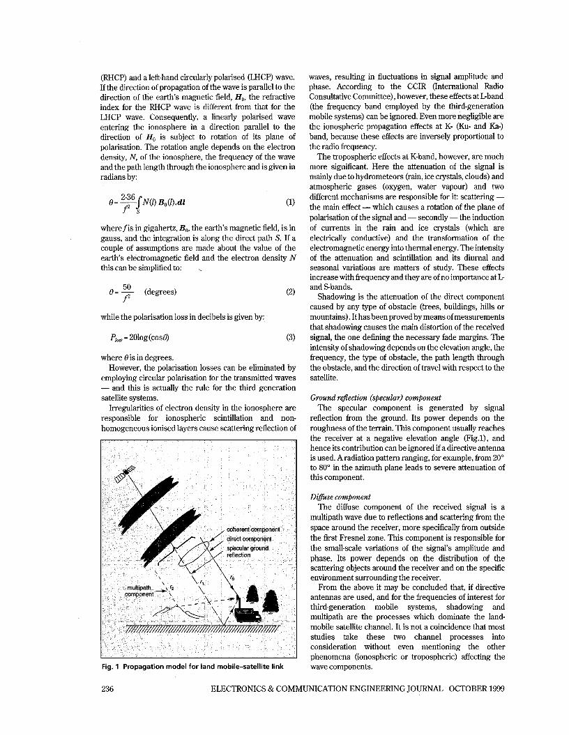
The received signal may be modelled as the sum of three components: two coherent (the direct and ground- reflected waves) and one incoherent (the diffuse ~ a v e ) ~ , ~ .

The direct component The direct component is received through aline-of-sight

(LOS) path, hence it is subject to free-space attenuation, Faraday rotation and scintillation due to the ionosphere, attenuation and depolarisation due to the troposphere, and shadowing.

Faraday rotation is the rotation ofthe polarisation axis of a non-circularly polarised wave. A linearly polarised wave is the vectorial sum of a right-hand circularly polarised

ELECTRONICS & COMMUNICATION ENGINEERING JOURNAL OCTOBER 1999 235

(RHCP) and a left-hand circularly polarised (LHCP) wave. If the direction of propagation of the wave is parallel to the direction of the earth's magnetic field, H,, the refractive index for the RHCP wave is different from that for the LHCP wave. Consequently, a linearly polarised wave entering the ionosphere in a direction parallel to the direction of H, is subject to rotation of its plane of polarisation. The rotation angle depends on the electron density, N, of the ionosphere, the frequency of the wave and the path length through the ionosphere and is given in radians by:

2.36 @ = -JN(l) B,(l).dl

f2 s

where f is in gigahertz, B,, the earth's magnetic field, is in gauss, and the integration is along the direct path S. If a couple of assumptions are made about the value of the earth's electromagnetic field and the electron density N this can be simplified to: .

(2) 50 e= - (degrees) f2

while the polarisation loss in decibels is given by:

Pr, = 201og(cos@) (3)

where @is in degrees. However, the polarisation losses can he eliminated by

employing circular polarisation for the transmitted waves - and this is actually the rule for the third generation satellite systems.

Irregularities of electron density in the ionosphere are responsible for ionospheric scintillation and non- homogeneous ionised layers cause scattering reflection of I I

Fig. 1 Propagation model for land mobile-satellite link

waves, resulting in fluctuations in signal amplitude and phase. According to the CCIR (International Radio Consultative Committee), however, these effects at Lhand (the frequency band employed by the third-generation mobile systems) can be ignored. Even more negligible are the ionospheric propagation effects at K- (Ku- and Ka-) band, because these effects are inversely proportional to the radio frequency.

The tropospheric effects at K-band, however, are much more significant. Here the attenuation of the signal is mainly due to hydrometeors (rain, ice crystals, clouds) and atmospheric gases (oxygen, water vapour) and two different mechanisms are responsible for it: scattering - the main effect - which causes a rotation of the plane of polarisation of the signal and - secondly - the induction of currents in the rain and ice crystals (which are electrically conductive) and the transformation of the electromagnetic energy into thermal energy. The intensity of the attenuation and scintillation and its diurnal and seasonal variations are matters of study. These effects increase with frequency and they are of no importance at L and Sbands.

Shadowing is the attenuation of the direct component caused hy any type of obstacle (trees, buildings, hills or mountains). It has been proved by means of measurements that shadowing causes the main distortion of the received signal, the one defining the necessary fade margins. The intensity of shadowing depends on the elevation angle, the frequency, the type of obstacle, the path length through the obstacle, and the direction of travel with respect to the satellite.

Groand reflection (specular) component The specular component is generated by signal

reflection from the ground. Its power depends on the roughness of the terrain. This component usually reaches the receiver at a negative elevation angle Fig.l), and hence its contribution can be ignored ifa directive antenna is used. A radiation pattern ranging, for example, from 20" to 80" in the azimuth plane leads to severe attenuation of this component.

Difise component The diffuse component of the received signal is a

multipath wave due to reflections and scattering from the space around the receiver, more specifically from outside the first Fresnel zone. This component is responsible for the small-scale variations of the signal's amplitude and phase. Its power depends on the distribution of the scattering objects around the receiver and on the specific environment surrounding the receiver.

From the above it may be concluded that, if directive antennas are used, and for the frequencies of interest for third-generation mobile systems, shadowing and multipath are the processes which dominate the land- mobile satellite channel. It is not a coincidence that most studies take these two channel processes into consideration without even mentioning the other phenomena (ionospheric or tropospheric) affecting the wave components.

236 ELECTRONICS & COMMUNICATION ENGINEERING JOURNAL OCTOBER 1999

3 Channel modelling Table 1: Parameters of the three different versions of the MED model

The objective of LMS channel a” Frequency range, MHz Study

modelling is to understand the 0.187f02qp41*. o D , ~ 400 m 200 5 f 5 95000 propagation phenomena which

Weissberger . . -

0 s D, s 400 m 200 5 f 5 95000 dominate the LMS channel and to derive rules and exoressions

0.Zf03DD;04

0.187f0284Dv44’2, 14s D,s400 m which describe the dependence of the received signal on a

CCIR

number of parameters: frequency, elevation angle, antenna twe and directivitv. relative

0,063f0 284, O S D , ~ 14m no reference Barts and Stutzman

.. velocity between receiver and satellite, type of environment.

Extensive measurement campaigns at UHF and, especially, at L and Sband - the bands allocated to the third-generation satellite systems- have formed the basis of attempts to model the LMS channel by various researchers all over the world. More recently measurement campaigns at K-band have been reported. Aircraft, helicopters and, in the best case, satellites have been employed in simulating the LMS channel.

The overwhelming majority of the models that have been derived are narrow-band models; this is not surprising in view of the fact that the third-generation mobile systems, which were the focus of attention at the time the work was carried out, are narrow-band systems. However the objective of the fourth and subsequent generation systems is to provide multimedia services similar to those that B-ISDN (broadband ISDN) will offer in fixed communication networks. These systems will be capable of providing much wider bandwidth channels - sufficient not only for voice but also for video services - justifying their characterisation as wideband systems. Most of the co-ordinated European research in this direction is being conducted within the SECOMS/ ABATE project. Much more interest in these systems, including their wideband effects, is expected in the next few years.

4 Narrow-band models

The narrow-band models reported in the literature can be classified into three main categories: empirical, statistical and analytical. There has been limited interest over the last five years in empirical modelling, though it attracted a lot of attention in the period 1985-92. There have also been few reports of studies concerning analytical modelling, though there are several papers referring to the terrestrial channel. Statistical modelling seems to have been the favourite modelling approach over the last 10 years.

A: Empitical models

Empirical models typically represent a curve fitted to measured data. The considerable advantage of empirical models is the simplicity of the final mathematical expressions which describe them and, hence, their easy application. However, they are strictly related to specific

measured data and fail to give any indication as to the physical processes involved in propagation within the channel.

These models refer either to the mean attenuation caused by vegetation or to calculation of the link margin needed to compensate for propagation losses and fades (fade margin). Various parameters are used in these models, including the elevation angle, 0, the frequency,f; the path length throughvegetation and parameters closely related to the specific environment in which the measurements were made. These parameters are nearly always computed through regression fits to the measurement data.

In the following presentation the classification of the models proposed in Reference 6 has been adopted. A comparison between the various models can also be found in that paper.

Models computing the vegetative attenuation Modzjied exponential decay (MED): This model

computes the mean path loss through vegetation taking into account the path length through the vegetation, D,, and the frequency,f: It is given by the equation:

Lo = a J L (4)

where L, is the attenuation in decibels, D, is in metres and a , is a coefficient called the ‘specific attenuation of the vegetation’ in decibels - a rather improper characterisation as it is a function of bothfand D,. The specific model was first introduced by Weissberger, was later simplified by the CCIR and, finally, was modified by Barts and Stutzman. Aslightly different expression for a, is given by each of the three studies, see Table 1.

The path length D, is computed taking into account the path geometry. Roadside vegetation is modelled as a uniform slab of height H and mean distance W from the vehicle. The path geometry is depicted in Fig. 2 and the expression for D, is:

D, = HcosecB- Wcosecysece (5)

The elevation angle 9 is assumed to be constant and that limits the validity of the model to use with geostationary satellites. The bearing angle y is constant for a straight road, while the height ofthevegetation and its distance, W, from the vehicle are uniformly distributed variables in a range defined hy a minimum and a maximum value.


Fig. 2 Path geometry for the computation of D,

Vogel and Goldhirsh model: Vogel and Goldhirsh have conducted a series of measurements for different environments (rural, suburban and urban) and frequencies. They evaluated attenuation at 870 MHz due to trees, employing either a remotely piloted aircraft or a helicopter as the transmitter platform.They extended their experiments to Lband and studied the influence of elevation angle (for angles of 30", 45" and 60") on path loss and fade; almost concurrently they performed measurements in mountainous regions and demonstrated that the required fade margin is basically defined by (tree) shadowing rather than multipath fading. Inmarsat's geostationary satellite Marecs B2 was used for the measurements at Lband, which yielded the ERS model mentioned below.

Based on their measurements for attenuation due to roadside trees, they introduced the following model, which predictstheattenuation,A, due to asingletree asafnnction of elevation angle 8:

A(0) = 0,480 + 26.2 (full foliage season) A(#) = 0.350+ 19.2 (bare treeseason)

(6) (7)

where A is measured in decibels and 0 is the elevation angle in degrees. The model is valid for elevation angles from 15' to 40".

They also examined the effect of seasons and foliage on the attenuation and derived the empirical relation:

A(fu1lfoliage) = 1.35Abaretree) (8)

This relation is valid for 15" s # 5 35" and for L- and S bands. It shows thatfoliage increases the attenuation of the bignd by a little over 1 dB. However, the influence of foliage upon signal attenuation is much more important at Ka- band it is reported in Reference 7 that it may cause an extra fade of -17 dB.

Models computing the link margin Appropriate power margins are required in land

mobile satellite links to compensate for propagation losses and fades. These margins are functions of parameters such as frequency and elevation angle and vary with the specific environment and even with the

season of the year. CCIR mode1:According to the CCIR (International Radio

Consultative Committee) model, which is based on measurement data at UHF and Lband, the link margin in decibels is given by:

M = 174 + 1.93f- 0.0520 + K(7.6 + 0.053f+ 0.040), (9) 19" s 0543'

for urban areas, and by

M = 12~5+0~17f-0~170+K(6~4-1~19f+0~058), (10) 19" s 0543"

for suburban/rnral areas, where #is the elevation angle in degrees, f is the frequency in gigahertz and K is the percentage of locations at which the carrier power is exceeded. Typical values for K are:

K(50%) = 0, K(90%) = 1.3, K(95%) = 1.65, (11) K(99%) = 2.35

The following three models introduce the general expression:

M=-Aln(P) + B (12)

for the computation of the required link margin. However, each model gives slightly different definitions for the parameters in this equation and also for their range of variation. In the following, Mis the required link margin in decibels for a given link outage probability Pin percent,fis the frequency in gigahertz and 8 is the elevation angle in degrees.

Empirical Roadside Shadowing (ERS) model: In addition to their previously mentioned (vegetation attenuation) model Vogel and Goldhirsh have proposed a model for computation of the link margin. The model is basically suggested for Lband (1.5 GHz), but it can become valid at both UHF (890 MHz) and Sband (2.6 GHz) if the frequency scaling factors mentioned below are applied. In this model the expressions for A and B, valid for 20" L # 5

60", are:

A=3~44+0.09750-0402#2 B = -0.443#+ 34.76

andPvariesfrom 1% to 20%. Modified Empirical Roadside Shadowing (MERS): This

model is valid for Lband and lor elevation angles ranging from 20" to 80". In this case:

A = 1~117x104#2-0~07018+6~1304 (13 B= 0~003202-0~66120+3723581 (16)

and Pis assigned values in the range 1-30%. Combined Empirical Fading Model (CEFM): In this

mode1,AandBarefunctionsofboth thefrequencyandthe elevation angle, rendering the model directly valid for L band (1.3 GHz) and Sband (2.45 GHz). The appropriate


expressionsforA andB,validfor20° s Bs So", are:

A = 0.00282 - 0.158-0.7-0.2f (17) B = 27.2 t 1.5f-0.338 (18)

and Pvaries from 1% to 30%. Frequency scalingfucto~; Vogel and Goldhirsh have also

derived a formula to compute the vegetative attenuation at different frequency bands. According to this formula:

~ v 3 = n v U H F ) E (19)

where AlfJ is the attenuation at L-band (1.5 GHz) and AVuHF) is the attenuation at UHF (870 MHz) in decibels. A similar relationship allows the attenuation at Sband to be calculated if the attenuation at L-band is known. Moreover, based on measured data they derived a different formula for the transition from L- to K-band attenuation and vice- versa:

where A(fi) and A@ are the attenuation in decibels at frequenciesf, andf,, respectively, expressed in gigahertz, and b=1.173. This formula is valid from 870 MHz to 19.6 GHz and yields a maximum error of 0.2 dB for the transition from L to K-band and 0.1 dB for the reverse transition (K- to Lband) .

A model-formula for computing the vegetative attenuation at Sband with reference to the attenuation at L- band has been derived by ESTEC, the European Space Research and Technology Centre:

A&) = 1.4lAVJ (21)

wheref, = 2.6 GHz andfL = 1.3 GHz.

B; Statistical models

In contrast to the empirical models, the statistical models offer an insight into the physical processes taking part in the propagation and reception of a signal. However, they usually, if not always, require the use of numerical analysis methods to overcome the computational d~cul t ies . The modelling work is directed primarily at defining the probability density function (PDF) and the cumulative density function (CDF) of the envelope - and sometimes (of) the phase -of the received signal. The derivation of these statistics is fundamental for the computation of adequate fade margins. Fewer studies have been concerned with modelling second order statistics of the signal: the autocorrelation function of the signal, the statistics of fade duration and the level crossing rate (LCR) . However, most researchers compute these statistics, after processing the measured data statistically, because they are the basis for selecting the required modulation and coding techniques.

First order statistics There are two different modelling approaches for first

order statistics, namely global and stateoriented statistical modelling. The former approach describes the channel conditions by a single distribution with its corresponding parameters, i.e. both shadowing and multipath are included in a single distribution.

In the stateoriented approach each of the several discrete states which the channel can have is described separately by a single distribution. This approach is supposed to describe in more detail the shadowing and multipath phenomena'.

Global statistical channel modelling: The log-normal distribution is widely - if not exclusively - used to describe large-scale fading, i.e. variations of the signal amplitude due to attenuation caused by any type of obstacle impeding the LOS path.

The distribution employed for describing small-scale fading - attributed to multipath effects - depends on the scattering environment and the assumptions made about the components of the received wave. The usual, though vague, classification of environments is into urban, suburban and rural environments. A rural environment implies the existence of an LOS path, allowing part of the signal to reach the receiver without being reflected or scattered. An urban environment on the other hand usually excludes the existence of an LOS path; the receiver is surrounded by a large number of scattering objects and multipath is the main - if not the only - propagation mechanism.The suburban environment is an intermediate category of environment, combining characteristics of both the urban and rural environments.

Hence, in urban environments, multipath is well described by a Rayleigh distribution. The use of the Rayleigh PDF implies that an infinite number of scattering elements contribute to the resultant wave. Some researchers, however, have assumed a limited number of scattering objects and derived different distributionsg. In rural and suburban environments, where an LOS component exists for most of the time, Rayleigh fading turns into Ricean fading.

The resultant PDF, which aims to describe both small- and large-scale fading, is nearly always a combination of the relatively simple distributions mentioned above and is called a 'mixture' distribution. Suzuki was the first to propose using 'mixture' statistics to describe the urban terrestrial mobile channel. His PDF for the envelope, r, of the received signal consisted of Rayleigh and log-normal statistics:

where 2 a 2 is the average received power of the Rayleigh process included in this formula, d is the standard deviation of the normal variable related to the log-normal process (see the Appendix), and p is the mean value of the normal variable related to the log-normal process

In the 20 years that have elapsed since the introduction of the Suzuki PDF and the almost concurrent study of Hansen and Meno, several models have been proposed which employ mixture distributions; the overwhelming


Table 2: Processes and probability density functions of the global models

Model Complex channel process, Envelope PDF r = r, + ~r , ,

Loo'O r = Sd+o + Rdm (In s - p)2 (r2 + s2) S : log-normal p,(r) =d+$,-p c T- R : Ravleiah distributed

I -

po,p: uniform

RLN'2 r=RSe'' S : log-normal R : Ricean distributed e : uniform

GRLN" r = RSd8 + x1 + jyl S : loa-normal R : Rizean distributed xl, y1 : Gaussian

Poca- r = RS@ lognormal9 5 : log-normal

R : Poca-log-normal distributed

e : uniform d hd' ) 2 ) (6 + SZd(2n + 1) 1 Ins-hu' r2

Patzoldetal" r=Se''2"'p'+np'+x1 +jyl S : log-normal xl, y, : Gaussian distributed f, and 0, : constant

majority of these employ Rayleigh, Rice and log-normal statistics. These models are tabulated in Table 2 and are compared below.

Firstly, for reasons already mentioned all models ignore the so-called specular component of the received wave. They take into consideration only the direct component and the diffusemnltipath component, which relates to the multipath effects of the channel. Moreover, all the models use log-normal statistics for the shadowing effects with parameters p and d or - alternatively - hp' and hd' (see the Appendix).

The main differences between the models arise (from a purely physical viewpoint) from the various assumptions that are made about the way the channel affects the direct and diffuse components, and this results in all the complicated 'mixture' PDFs given in Table 2.

For his model Loo" assumed that only the direct component suffers from shadowing, and that the diffuse component has constant power. This is obvious in the mathematical expression describing the channel process, r, in which the sequence S corresponding to the direct component (log-normal envelope) is added to the sequence R representing the diffuse component (Rayleigh envelope).

Patzold et uZ." seem to agree with Loo's hypothesis: they derived an exactly similar distribution for the envelope PDF. However, in order to enhance the flexibility of their model, they made two extra assumptions :

they allowed the inphase and the quadrature components - xl and yl, respectively - of the diffuse process to he cross-correlated they assumed that the direct component is Doppler shifted If,), thereby providing an additional degree of freedom for adapting the second order statistics of the model to the measured data.

In their Rice-log-normal (RLN model, Corazza and Vatalaro" assumed that shadowing affects the two components in the same way. The power of the diffuse component is no longer constant, as the diffuse component suffers exactly the same variations as the direct component. This can he seen io the mathematical description of the model: the two components are no longer discrete but are incorporated in a Ricean process, R shadowing - represented by a log-normal process, S - acts multiplicufively to this Ricean process. The parameter c refers to the Rice factor, which is defined as:

7: c=P

where U' is the mean received power of the diffuse component and r,"/2 is the power of the direct signal component; I, is the zero-order modified Bessel function.

In contrast, Hwang et ubI3 do not assume any correlation between the shadowing processes affecting the two signal components. The shadowing, S,, of the direct component,


A,, is not related to the shadowing, S,, suffered by the multipath component, R. The two log-normal processes SI and S, are independent and have different parameters. Nevertheless, owing to its many degrees of freedom, this model can include the previously discussed models as special cases if appropriate values are assigned to its parameters. If the previous models were characterised by means of a correlation coefficient between the direct and diffuse component^'^, this would be zero for the Loo and Patmld et al. models, which assume no shadowing for the multipath component, as well as for the Hwang et al. model, which takes shadowing of the multipath component into account but accepts no correlation with the shadowing affecting the direct component. In contrast, the coefficient would be unity for the RLN model. The generalised RLN (GRLN) model'' is a compromise between the two extfeme, contradictory assumptions of the previous models. According to the GRLN model, the diffuse component is divided into two parts: one that suffers from shadowing and one that has coustimt power. This is obvious in the model's mathematical des'aiption. The process R, with a Ricean envelope, is multiplied by the log-normal variable S and the resulting product is added to the zero-mean complex Gaussian processzl+&, which has a Rayleigh envelope. By altering the value of the parameter E defining the relative power of the two parts of the diffuse component, Vatalaro'5 attempted to describe a variety of situations lying between the two extreme cases (correlation=O, correlation=l), although a direct relationship between values of 5 and specific values of correlation is not possible. The parameter cis the Rice factor mentioned above (eqn. 23).

Finally the Poca-lognormal model assumes that there is only a diffuse component and that this suffers from shadowing. Its originality lies in the application of a new distribution for describing fading effects. Using a study of indoor channels and assuming that the number of scattering objects is not infinite (the Rayleigh distribution assumes an infinite number) but rather small (45 , for example), the authors of this modelg propose the so called Pocadistribution, which seemsto be ageneralisation ofthe Rayleigh distribution. In their expression for the envelope PDF given in Table 2, K,, is defined as:

where v = 3, 5, 7... is the number of the dominant propagation paths; U is the parameter of the Paca distribution, which is closely related to the received signal power, and r() is the well-known gamma function.

Typical envelope PDFs for the global models of Table 2 are illustrated in Fig. 3.

The mixture PDFs, however, are not always adequate for describing the LMS channel, especially in the case of LEO and ME0 satellite constellations, where the variability rate of the channel is high. The frequent changes in the elevation angle of the satellite generate different propagation conditions, which succeed one another rapidly and cannot be modelled by a single distribution. This potential failure of a single PDF to

Fig. 3 Envelope PDFs of the global models of Table 2 for typical parameter values

describe the channel effectively because of the channel's enhanced complexity led to the development of state oriented modelling.

Stute+riented channel modelling: In this approach a Markov process is used to model long-term variations of the channel and its transitions to different states; short- term variations - corresponding to each individual discrete state - are described by one of the above mentioned PDFs with apropriate parameters.

A Markov process is a stochastic process in which a system can take on discrete states in such a way that the probability of taking on a given state depends only on the previous state. Two matrices must be computed to d e h e the process completely:

0 the lxMstate probability m a y W, whose elements, W,, express the probability of the system being in state i (i =

l..N 0 the MxM transition probability matrix P, whose

elements Pijgive the probability of transition from state i to statej.

A threcstate Markov chain is illustrated in Fig. 4. The number of states of the Markov chain as well as the statistics describing each of these states differ from model to model and from researcher to researcher. Lutz et al.'6 introduced a two-state model, while Karasawa et al.'? and Fontan et al.' proposed a three-state model. Vucetic' has suggested that a four-state model is adequate for experimentalpurposes. lfanM-statemodelisusedandpiis the PDF describing the ith state then, by application of the total probability theorem, the total PDF of the model is:

M

P , ~ , = w 9 1 + w ~ , + . . . + w o 4 ~ = c P i w i (25)

where wi are the elements of the array W. Lntz et al.'6 conducted a broad measurement campaign

in several European cities, exhibiting elevation angles from 13" to 43".Their efforts tostudy multipath shadowing

ELECTRONICS C COMMUNICATIQN ENGINEERING JOURNAL OCTOBER 1999 241

Fig. 4 A three-state Markov chain

and signal attenuation in different environments, and hence under different propagation conditions, yielded a new model - the DLR (Deutsches Zentrum fiir Luft- und Raumfahrt) model - whose main assumption is that the channel can fall into one of two discrete states.When there is no shadowing - the ‘good state’ - the envelope of the received signal follows the Ricean PDF, while under shadowing conditions -the ‘bad state’ - the envelope of the received signal is a Rayleigh process with a log- normally distributed mean value. The most important parameter ofthe model is the timeshare of the shadowing, A. The resulting probability density function of the received signal power, based on the total probability theorem, is:

PP(P) = (1-4 P,e,(P) +ASP,,,(P/P,)Pi~(P,)dP, (26) 0

In comparison with the general form of the state-oriented models, the state probability matrix of the DLR model consists of two elements, A and I-A, while the state transition probability matrix is reduced to a 2x2 matrix. Lutz et al. estimated the appropriate values forA, p’, d‘ and c for several cities and environments (rural, suburban, urban), based on corresponding sets of measurement data and methods of linear regression fits. Based on the results of the same experiment and applying the least squares fit, Parks etal. proposedan empirical formulafor estimatingA as a function of elevation angle B:

A =0.981497- 0,01219568- 5.077828’ (27)

This formula is applicable for suburban environments. A different approach, with the advantage of relating A

to the physical environment of the measurements, thus assigning a less abstract meaning to it, is given by Saunders and EvansI8. They estimated A, or p ( 3 as they call it, for a standard point with reference to a simple geometrical model, taking into consideration the distribution of the heights of the surrounding buildings

and the geometry of the specific environment, including the elevation angle. The method is valid for GEO channels, where the elevation angle can be assumed constant.

After performing Lband measurements in urban Japan at an elevation angle of 32”, Kavasawa et al. proposed a model which takes into account three discrete states. The signal envelope is described by a Ricean distribution when the LOS component is clear of obstacles, and by a Loo PDF when the LOS component is shadowed. The third state, corresponding to complete blockage of the LOS by buildings, follows a Rayleigh PDF. Therefore the cumulative probability function - in agreement with the total probability theorem - is a weighted linear combination of Ricean (0, Loo (S,) and Rayleigh (B) processes:

PLY) = CPRidY) + ~kP,(v) + BPkb,(Y) (28)

where the parameters for the three distributions as well as the weighting factors are computed by fitting to the measured data. It is obvious that C, S, and B correspond to the elements of the (in this case) 1x3 array W.

Apart from the usual method of linear fitting to measurement data, an alternative method for computing the weighting factors introduced in Karasawa et al.’s model has been presented by Vogel and Akturan”. They made use of photogrammetry and image processing algorithms to define the percentages of the time corresponding to each of the three states, assigning an insight to the physical hypostasis of these factors and their relation to the surrounding environment and elevation angle.

After processing measured data at Sband, Fontan et al. presented athreestate model based on Markov processes. The three states taken into account were:

State 1: h e of sight (LOS) conditions State 2: moderate fading conditions State 3 deep fading conditions.

The measured data were filtered with a low-pass filter, so that the shadowing influence was removed, and then classified into the three abovementioned states.

The elements of the arrays W and P (necessary for realisation of the Markov process) were estimated by the following ratios:

Wj = NJNj (29)

where Ni is the number of samples corresponding to state i and N, is the total number of samples;

Pjj = Njj/Nj (30)

where Nij is the number of transitions from state i to state j and N, is the number of samples corresponding to state i. Loo’s statistics were used to describe all three states, with different parameters for each state, defined by fitting to measurements.


A slightly different approach - also employing Markov statistics - was introduced by WakanazO. His model contains two main states: the fade slate and the non-fade state. However the fade state is divided into two substates, onewithasmallerandonewithalongerduration.Similarly the non-fade state includes three substates of short, long and much longer duration. The two fade states are modelled by Rayleigh statistics, while the three non-fade statistics are Ricean distributed. No transition between different fade or non-fade states (substates) is allowed, hence the 5x5 transition matrix includes 8 zero elements. Instead of deriving a theoretical expression for the PDF of the resultant model, Wakana was interested in the fade duration produced. By employing an exponential function for the fade duration and a log-normal function for the non- fade duration, he showed an excellent match between his model and measurements of fade duration performed in Australia by other researchers.

Second order statistics LCR andAFD: In his study ofthe statistical properties of

noise, Rice defined the level crossing rate (LCR), N,, at a specific level r = R as the expected rate at which the envelope crosses that level in a positive-going direction. This definition is interpreted mathematically as:

where the overdot indicates a time derivative andp(R, Y ) is the joint probability density function of the envelope rand its derivative 9 at r = R.

The average fade duration (AFD) under a specific level r = R is the mean duration of the intervals during which the envelope falls below the specific level. 1fz;is the duration of the ith fade interval, the probability that r i R during a time interval Tcan be written as:

1 T i

P ( r i R ) = - z z ,

and the AFD, t, is given by:

(33)

These channel system parameters, i.e. the LCR and AFD, can be extremely interesting. The AFD, for example, is of particular interest in defining the optimum interleaver and forward error correcting (FEC) codes to use in receivers for the mitigation of fading effects. Bearing in mind Rice's studies, Loo made two important observations. He showed that if the log-normal component - refemng to the direct wave component - is assumed to be constant, and hence that the signal undergoes Ricean fading, then the rate of change of the envelope, Y , is uncorrelated with the envelope of the signal. Therefore:

P(r, 9) =p(r)p(f) (34)

wherep(r) is a Ricean distribution, as expected, whilep(i) is Gaussian distributed.

A similar result was derived, when the d ~ s e component was ignored and only the log-normally distributed direct componentwas taken into consideration.Therate ofchauge of the envelope was again found to be Gaussian distributed, although the envelope now followed the log-normal distribution, while the condition 34 was also valid. In view of this eqn. 31 can be simplified to:

rn

NR = p (r) $i p (Y)dY (35)

In view of these observations, Loo made the assumption that the rate of change of the envelope, Y , can be expressed as the sum of two correlated zero-mean Gaussian random processesi andjr, that is:

0

Y =i + j r (36)

Using a simple transformation it is then easy to find the distributionofp(9) and tocomputetheintegralineqn. 35 to give the following final expression for N,:

d G ? bz (b2 + 2pdG2 + d2) 'I2

d% b 2 ( 1 - p ? + 4 p d u 2 NR= ~ P (r) (37)

where p(r) is the envelope PDF according to Loo's model, db2 and dd2 are the standard deviations of the Gaussian processes i and y , and p is their cross-correlation coefficient.

Making a final assumption that the fading spectrum due to shadowing and multipath is symmetrical, expressed mathematically as:

wherefd,, is the maximum Doppler-shift frequency, the normalised NR - independent of fd,, - was computed to be:

fdm,

The average fade duration is immediately given by eqn. 33 as:

Fade and nonfade duration: Instead of deriving expressions for the cumulative distribution of the average fade duration theoretically, as in the hvo studies mentioned above, Hase, Vogel and Goldhirsh" relied on measured data to describe the CDF of fade and non-fade durations. The experimental data were best fitted by curves following the log-normal and the power law, respectively.


The fade state was defined as those periods of time during which the signal level was below a certain threshold, the non-fade state being the rest of the time, during which the signal exceeded the defined threshold. It was found that when the fade threshold value ranged from 2 to 8 dB, the CDF of the fade (dF) and non-fade (dG) durations, measured in metres, were given from:

and

P(d,,F>X) = b ~ " (43)

respectively, where a, b, c and uF are parameters computed using statistically processed measured data.

Correlation ofshadowfading: Measurements at elevation angles of 60" and 80" were the basis for the correlation model described in Reference 22. This model is for shadowing processes that cause largescale variations of the signal. For this reason, the measured data were passed through a lowpass filter that was narrow enough to average out the fast, small-scale variations of the signal caused by multipath yet wide enough to pass the slower shadow hding.Theoutputofthefi1terwasfound to bealog-normally distributed signal, implying that the signal strength in decibels is Gaussian distributed. The proposed model for the antocovariance Cs(t) of the shadowed signal S(t) is:

cS(z.) = E { s ( ~ ) S(t + z.1 } - ~2 ~ ( t ) I = osz e + '''e (44)

where U, is the standard deviation of S(t),X, is the effective correlation distance, defined as the distance at which the normalised correlation falls to e-', B is the velocity and t i s the sampling interval. X , was found to be of the order of 10 m (9-17 m for wooded and 1G20 m for suburban environments).

C:Analyticul models

The analytical models reported io the literature are mainly concerned with the terrestrial mobile channel. A brief review of these models is given in Reference 23. Little work dealing with the LMS channel has been reported.

Ossanna was the first person to work on analytical modelling of the mobile channel. He introduced a model which assumes that the resultant wave at the receiver is the sum of a direct and one or more reflected wave components. The main disadvantage of his socalled reflection model is its assumption that a direct component exists; this is not valid for urban environments, where propagation is chiefly due to scattering.

GilberP focused on the scattering process and proposed three slightly different models, according to which the resultant wave is the sum of N scattered waves. The amplitudes of the discrete components may be either (U) Rayleigh distributed with equal variance or (b) equal and constant or (c) randomly distributed the phase of the components is uniformly distributed in the interval (0,2n).

ClarkZ5introduced a scattering model based on the second scenario. According to this model the electric field is given by:

N

U t ) =~.E,exp0.i2nV;+fd,,,cosa3t+ / L #,I) (45)

where E, is the constant amplitude of the discrete components,fd,, is the maximum Doppler shift caused by movement of the mobile receiver with respect to the scattering objects, #cis the phase delay angle and a, is the horizontal angle of amval, both angles being uniformly distributed in the interval [O, 2x1.

The models mentioned above are two-dimensional. AulinZ6 introduced a three-dimensional model which assumes that the wave components do not just arrive at the receiver horizontally - an assumption which seems to be even more valid in the case of LMS channels, where the transmitter platform, namely the satellite, is placed much higher than the receivers. The above expression for the z- component of the electric field then becomes:

WO =E,explj[2nK+fdmcos ~ 1 3 t+ @,I) (46)

In comparison with eqn. 45, the horizontal angle a, is now replaced by q,, which can be analysed into the horizontal angle a, and the vertical angle p, of arrival (Fig. 5). The horizontal angle still follows a uniform distribution in the interval CO, 2x1 but the vertical angle p follows a different PDF:

(47)

Aulin derived similar expressions for the envelope and the phase of the received signal, which were Rayleigh 'and uniformly distributed, respectively, but the above three- dimensional concept gave a different signal spectrum, which showed better agreement with measured spectra.

Parsons andTurkmaniZ3 adopted Anlio's model butgave a different PDF for the vertical elevation angle of arrival, p:

This distribution effectively removes the spectrum discontinuities caused by the PDF proposed by Auliu.

All the references cited above analyse the received signal in terms of its amplitude, phase, auto- and cross- correlations.

Gilbert, Clark, and Aulin proposed expressions for the z component of the electrical field, E,, because they initially assumed that the transmitted signal was vertically polarised. Onlyone study dealingwith analyticalmodelling of the LMS channel has been reported, however this does not take into account the circular polarisation of the transmitted signal. In his PhD thesis, A. Kanatas introduced a scattering model for the LMS channel which follows Aulin's concept. The motion of the satellite with respect to the scatterers, which are assumed to be k e d ,


generates a Doppler shift, fds,.,:

fds,, = Vd/ l (49)

where Vd is the radial velocity of the satellite with respect to the fixed scatterers and I is the wavelength. Consequently all the scatterers can be regarded as transmitters of the signal at the kequency f,+fd,,. The receiver collects the components from each scatterer, the components arriving at horizontal angles ai, which are uniformly distributed in the interval 10, 2n1, and vertical angles Oj, which are distributed according to eqns. 47 or 48. The expression suggested for E, is almost identical with eqn. 4 6

E,(t) =E, exp j 2a f,+fds,fifdm, 1+ - cos vi t+@i (50)

where c, is the velocity of the electromagnetic field in free space. Computation of the power spectral density (PSD) of the signal yields the same U shape as the PSDs derived from eqns. 45 and 46. However, to date no measurement data have been reported which confirm the assumptions made in this model.

5 Wideband models

The main approach to the modelling of wideband effects, both for terrestrial and satellite mobile channels, is via the study of the impulse response of the channel. If it is assumed that there are a discrete number of scattering generators surrounding the receiver and that the geometrical optics approach isvalid, then the time variable impulse response, h (t,z), of the channel can be written as:

h(t,d = x A j ( t ) S( t - t j ( t ) ) ejai(') (51)

where Ai@), xi@) and Q(t) are the random time-varying amplitude, arrival time and phase sequences, respectively, S is the delta function and N-1 is the number of scattered wave components taken into consideration. The term fori = 0 corresponds to the direct component - when there is one - while the other N-1 terms represent the echoes which amve at the receiver due to multipath.

The expression for the channel impulse response clearly implies that it can be modelled by a tapped delay line (Fig. 6). In fact this approach has been widely accepted and employed by the overwhelming majority of investigators of the terrestrial mobile channel. The several models proposed aim at defining suitable distributions for the amplitudes Ai (the tap gains), the delay times 4. and also the Doppler spectra of each tap or the time correlation of each discrete path (tap) gain.

The same approach is encountered in the few studies that have dealt with the LMS channel. The choice of the relative distributions for each model and the number of path-taps for efficient modelling is based on measurements and statistical analysis of measurement data.

The DLR (German Aerospace Centre) model

{ [ ( ( 3 ) 1

H-l

(4

Jahn employed a tapped delay line with 3,3 and 5 taps,

Fig. 5 Scattering geometry for analytical modelsz3. a, is the horizontal angle of arrival; is the vertical angle of arrival

respectively, for modelling the three different channel environments - rural, suburban and urban. He suggested distributions for the amplitude gains, the delay times and the Doppler spectra of each tap. For the first tap - corresponding to the direct component - he employed either a Rayleigh or a Ricean PDF, according to whether the LOS path is shadowed or no$ for the other taps (echoes) he used a Rayleigh PDF. The Doppler spectra of the taps depend on the chosen distribution for the amplitude gains of the taps. When a Rayleigh PDF is employed for the tap gains, a Rayleigh Doppler power spectral density (PSD) describes the Doppler shift of the tap:

where jd,, is the maximum Doppler shift, related to the speed, om, of the mobile terminal by:

fd,, = %/I (53)

jd,, is the Doppler spectrum shift due to the velocity of the satellite relative to the earth's surface (eqn. 49) and um2isthe mean power of the corresponding Rayleigh process. The DopplerFSD ofeqn. 52isalsoknomasJakesDopplerPSD.

Similarly, ifa Rice PDF is employed for the tap gain, then the Doppler shift of the tap corresponds to a Ricean Doppler spectrum, consisting of the Jakes power spectral density weighted by the inverse of the Rice factor plus a discrete spectral line:


Table 3: Comparison table of global models with regard to the correlation coefficient

Complementary comments and refere

Loo (1985) zero Shadowing affects only the direct component”

RLN (1994) unity Shadowing of both the direct and diffuse components’2

GRLN (1995) variable Part of the diffuse component is shadowed”

Hwang e t al. (1997) zero Shadowing of both the direct and diffuse component^'^

No direct component is assumed’ Poca-log-normal (1998)

Patzold e t a/. (1998) zero Diffuse power = constant”

where c is the Rice factor. The extra spectral line relates to the Doppler shift of the direct component. An analytical report of Jahn’s conclusions and models can be found in Reference 27.

The CCSR-ESTEC model On hehalf of the European Space Research and

Technology Centre (ESTEC), researchers at the Centre for Communication Systems Research (CCSR) at the University of Surrey examined five different environmental categories at elevation angles in the range 15”40” using the results of a measurement campaigd4. The delay spread at Lband and Sband was the main parameter investigated in this experiment and several empirical expressions were derived. Parks et al. found that the typical average delay was 120-150 ns, which is smaller than the values reported in studies concerned with the terrestrial channel.

Si taps were chosen for implementing the tapped delay line, each tap being described by its timevarying amplitude and the corresponding Doppler spectrum. A Ricean distribution was employed in the statistical description of not only the first tap amplitude (corresponding to the direct component) but also the second tap amplitude. This choice of distribution was suggested by the results of statistical analysis of the measured data and convincingly explained by the authors: the first echo is usually attributed to discrete scattering elements placed near the receiver and not to a large number of uncorrelated scatterers, which would generate a Rayleigh-distributed echo. The four other taps were modelled by Rayleigh statistics. The parameters of the

Fig. 6 Tapped delay line modelling of the time-variant response of a channel

distributions were defined in accordance with the measurement results, so that this general model structure can describe the whole variety of environments and elevation angles that were examined.

Saunden et al. Based on these studies Saunders et dZ8 introduced a

slightly different approach to the study of the LMS channel. The channel is divided into two segments: the satellite-to-ground segment and the terrestrial segment. The former is represented by an attenuation factorA and a Doppler shift& due to the satellite’s motion relative to the earth‘s surface. The latter is further divided into two parts: the line-of-sight (LOS) part and the multipath part (MP) (Fig. 6). The multipath part is modelled, as customary, by a tapped delay line. Clearly such an approach makes the multiple studies of wideband effects in the terrestrial mobile channel more valuable than the two approaches previouslyreferred to.

6 Conclusions

This paper has described the attempts to model the land mobile satellite channel - with reference to the third- generation satellite systems for mobile communications- that have been made since the late 1970s, when the first pertinent studies were reported.

Of the three general modelling approaches the statistical one seems to be the most popular, especially during the last eight years. The greater complexity of the analytical models and the poor physical background of the

246 ELECTRONICS & COMMUNICATION ENGINEEHNG JOURNAL OCTOBER 1999

empirical models has deterred most researchers from focusing their efforts on these two approaches. The lack of studies which exploit the fundamental theories of wave propagation, such as geometrical optics (GO) or the uniform theory of diffraction (UTD), is more than evident. In contrast, the statistical approach has proved attractive as it provides an insight into the physical phenomena of wave propagation and reception whilst avoiding the complexity of an analytical approach.

The preferences of researchers are less clear regarding the two methods of statistical modelling; although an increasing number of scientists are choosing the stateoriented method, the global-modelling approach has not been abandoned. At present there is more interest in finding methods of deriving model parameters that take into consideration the specific scattering geometry of the 1 10 -(lologs-tr 1 /U

receiver rather than using methods that simply adapt the model to the measured data by means of numerical analysis algorithms.

The proposed models have been derived on the hasis of measurement campaigns at specific locations. These were selected in as representative a manner as possible but this is not sufficient to render the models applicable to any environment. Consequently each model imposes its own restrictions on the demanded power margins and the modulation parameters and coding employed at the receiver. A comparison of the performance of four representative models is attempted in Reference 29, where the models are integrated into a complete transceiver simulator and the transmitted power as well as the depth of the employed interleaver vary.

Appendix

A variable v is said to follow the log-normal distribution when it is defined as: 1 -(2-!’1/U‘

Fig. 7 Representation of the LMS channel according to Reference 28

12, following alog-normal distribution can be proved to he:

(59)

where the parametersp’ and d‘ are related to the previous parameters p and d through a multiplicative factor h =

(ln10)/20,that is:

In 10 p=hp’=-

=- s d‘ I n l O x a e

(60) 20 2”’

and

(61)

Finally, it can be proved that the power of a log-normal variable in decibels is normally distributed. If the new variable is defined as P = l0logS = 101og?, a simple transformation gives the distribution of Pas:

In 10 20

d = hd‘ = - 8

(62) D(P)=-e

where Yis a normal variable with parameters:

and

0,2=E[(Y-F)ZI=& (57)

The PDF of the variable ris:

The normal variable Y is the one mentioned in the description of the parameters of the models.

The distribution of the ‘power‘ of avariable, defined as S =

where the parameters p’ and d‘ are still given by eqns. 60 and 61. This justifies the term ‘dB spread’ which is attributed to the parameter d‘ in some papers”.

References

1 ANANASSO, F., and PRISCOLLI, F. D:: “The role of satellites in personal communication services’, IEEE 1. Sel. Areas Commun., February 1995,13, (Z), pp. 180-195

2 EVANS, J. V.: ‘Satellite systems for personal communications’, Proc. IEEE, July 1998.86, (7). pp. 132S1340

3 RE, E. D.: ‘A coordinated European effort for the definition ofa satellite integrated environment for future mobile communications’, ItiEE Commun. Mag., February 1996, pp. 9 6 1 0 4

4 DAVARIAN, F.: ’Channel simulation to facilitate mobile satellite communications research’, IEEE Trans. Commun., January 1987,35, (I), pp. 47-56


5 WCETIC, B., and DU, J.: 'Channel modeling and simulation in satellite mobile communication systems', IEEE J. Sel. Areas Commun., October 1992,10, (8), pp. 1209-1218

6 KANATAS, G., and KONSANTINOU, P.: 'Narrow-band characterization of the land mobile satellit? channel: a comparison of the empirical models', Eur. Trans. Telecommun, July-August 1996,7, (41, pp. 315321

7 GOLDHIRSH, J., and VOGEI,, W. J.: 'Earth-satellite tree attenuation at 20 GHz: foliage effects', Electron. Lett., September 1993,29, (18), pp. 1640-1641

8 FONTAN, F. P., GONZALEZ, J. P., FERREIRO, M. J. S., CASTRO, M. A V., BUONOMO, S., and BAPTIST& J. P.: 'Complex envelope threestate Markov model based simulator for the narrow-band LMS channel', Int. J Satell. Commun., 1997,15, pp. 1-15

9 BABALIS, P. G., and CAFSALIS, C. N.: 'A new model for the characterization of the combined shadowing and multipath effects in satellite systems' ICT '98, June 1998, IV, (4), pp. 2 5 2 8

10 LOO, C.: 'A statistical model for a land mobile satellite link', IEEE Tfum. Vek. Technol., August 1985,34, (3), pp.122-127

11 PATZOLD, M., KILLAT, U., LAUE, F., and U, Y.: 'On the statistical properties of deterministic simulation models for mohile fading channels', IEEE Trans. Veh. Technol., February 1998,47, (l), pp. 254-269

12 CORAZZA, G. E., and VATALARO, F.: 'A statistical model for land mobile satellite channels and its application to nongeostationary orbit systems', IEEE Trans. Vek. Technol., August 1994,43, (3), pp. 73b741

13HWANG,S.H.,KIM,IC-J.,A",J.-Y.,andW"G,IC-C.:'A channel model for nongeostationary orbiting satellite systems'. Proc. IEEE Vehicular Technology Conf., 1997, pp. 4 1 4 5

14PARI<s, M. A. N., SAUNDERS, S. R., and EVANS, B. G.: Wideband measurements and modeling at L and Sbands of tbe mohile satellite propagation channel'. COST 252 TD (97)

15 VATALARO, F.: 'Generalised Rice-lognormal channel for wireless communications', Electron. Lett., October 1995, 31,

16 LUTZ, E., CYGAN, D., DIPPOLD, M., DOLAINSKY, F., and PAPKE, W.: T h e land mobile satellite Communication channel - recordings, statistics and channel model'. COST 227 TD (93)

17 KARASAWA, Y., MINAMISONO, IC, and MATSUDO, T.: 'A propagation channel model for personal mobile satellite selvices'. PIERS '94 Conf., Noordwijk, The Netherlands, 11th-15thJuly 1994

lXSAUNDERS, S. R., and EVANS, B. G.: 'Physical model of shadowing probability for land mobile satellite propagation', Electron. Lett., August 1996,32, ( l n , pp. 1548-1549

19AKTURAN. R, and VOGEL, W. J.: 'Photogrammetric mobile satellite selvice prediction', Electron. Lett, February 1995,31, (31, pp. 16S166

20 WAKANA, H.: 'Propagation model for simulating shadowing and multipath fading in land mobile satellite channel', Electron. Lett., November 1997,33, (23), pp. 19251926

21 HASE,Y., GOLDHIRSH,J.,andVOGEL, W.J.:'Fade-durations derived from land mobile satellitaneasurements in Australia', IEEE T~am. Commun, May 1991,39, (5), pp. 664-668

SZTAAGHOL, P., and TAFAZOLU, R: 'Correlation model for shadow fading in land mobile satellite systems', Electron. Lett., July 1997,33, ( 1 5 1 , ~ ~ . 1287-1288

23 PARSONS, J. I)., and TURKMANI, A M. D.: 'Characterization of mobile radio signals: model description', IEE Proc.-I, December 1991,138, (6),pp. 549-556

24 GILBERT, E. N.: 'Energy reception for mobile radio', Bell Syst. Tech. J., 1965,44, pp. 1779-1803

25 CLARKE, R H.: 'A statistical theory of mobile radio reception', Bell Syst. Tech. J., 1968, pp. 957-1000

26AULIN, T.: 'A modfied model for the fading signal at a mobile radio channel',IEEE Truns., 1979.W-28, (3), pp. 182-203

27BISCHL, H., JA", A, and LUTZ, E.: Wideband channel model for UMTS satellite communications'. DLR Oeutsches Zentrumfiir Luft-und Raumfahrt), ETSI / SMG 5 16, Paper No. ETSI SMG5 (96) TD 0W96.10 pp.

28TZARAS, C., SAUNDERS, S.R., and EVANS, B. G,: 'A tapgain process for wideband mobilesatellite PCN channels'. COST 252TD (97)

29 KARALIOPOULOS, M., and PAVLIDOU, F.-N.: 'Astudy of the land mobile satellite channel in the frame of 3rd generation satellite systems'. COST252 TD (98)

30 BRAUN, W. R., and DERSCH, U.: 'A physical mohile radio channel model', IEEE TvmxVeh. Teehnol., 1991,40, (2), pp. 472482

31 SAUNDERS, S. R., TZARAS, C., and EVANS, B. G,: 'Physical- statistical propagation model for mobile satellite channel'. C O S 2 5 2 T D (98)

32 LOO, C., and BU'TTERWOKTH, J. S.: 'Land mobile satellite channel measurements and modeling', Proc. IEEE, July 1998, 86, (7), pp. 1442-1463

( 2 2 ~ pp. 1899-19no

OIEE1999 First received 2nd November 1998 and in final form 22nd February 1999.


Documents

Modelling the land mobile satellite channel: a review