Embed Size (px)
Citation preview
263Ann. For. Sci. 61 (2004) 263–275© INRA, EDP Sciences, 2004DOI: 10.1051/forest:2004019
Original article
Modelling the biomechanical behaviour of growing trees at the forest stand scale.
Part I: Development of an Incremental Transfer Matrix Methodand application to simplified tree structures
Philippe ANCELINa,b, Thierry FOURCAUDa,b*, Patrick LACa
a Laboratoire de Rhéologie du Bois de Bordeaux, UMR CNRS/INRA/Université Bordeaux I, Domaine de l'hermitage, 69 route d'Arcachon, 33612 Cestas Cedex, France
b Programme Modélisation des Plantes, CIRAD-AMIS – AMAP – TA40/PS2, boulevard de la Lironde, 34398 Montpellier, France
(Received 18 July 2002; accepted 23 April 2003)
Abstract – Stem straightness defects are often associated with heterogeneities in wood structure in relation to tree tropisms. This paper presentsa numerical model which is dedicated to simulate the biomechanical behaviour of growing trees. A simplified description of tree structure,separating trunk and crown, has been used in order to perform future calculations at the stand level. The model is based on the Transfer MatrixMethod, which was adjusted under an incremental form to compute the evolution of trunk biomechanics during growth. Deflections due to self-weight distribution and straightening up reactions, which are associated with maturation strains of reaction wood cells, were considered. Thismodel has been implemented in the CAPSIS software. Numerical results were compared to those obtained by the software AMAPpara, whichis more applicable to the whole tree architecture level. Limits of the simplified description, which will be useful for studies at stand level, arediscussed.
biomechanics / negative-gravitropic response / reaction wood / stem shape / growth stresses
Résumé – Modélisation du comportement biomécanique d'arbres en croissance à l'échelle du peuplement forestier. Partie I :développement d'une Méthode Incrémentale des Matrices de Transfert et application au cas d'arbres simplifiés. Les défauts de rectitudedes tiges sont souvent associés à des hétérogénéités structurelles du bois via des phénomènes de tropismes. Cet article présente un modèlenumérique de simulation du comportement biomécanique des arbres en croissance. Une description simplifiée de la structure, considérantséparément le tronc et le houppier, a été adoptée afin de permettre des calculs futurs à l’échelle du peuplement forestier. Le modèle numériqueest basé sur une formulation incrémentale de la Méthode des Matrices de Transfert permettant de tenir compte de l’évolution de l’état mécaniquedu tronc tout au long de la croissance de l’arbre. Le modèle prend en compte les déformations dues au poids propre de la structure, mais aussiles phénomènes de redressement associés aux déformations de maturation du bois de réaction. Ce modèle a été implanté dans le logiciel CAPSIS.Les résultats numériques ont été comparés à ceux obtenus en utilisant le logiciel AMAPpara. Ce dernier utilise un modèle biomécanique reposantsur une description détaillée de l’architecture de l’arbre. Les limites d’une description simplifiée de la structure, qui sera utile pour des calculsà l’échelle du peuplement forestier, sont discutées.
biomécanique / réponse gravitropique négative / bois de réaction / forme des troncs / contraintes de croissance
1. INTRODUCTION
Stem shape defects are closely associated with tree biome-chanical behaviour. These defects are often linked with pitheccentricity and reaction wood formation. They have a hugeimpact on timber quality and hence reduce economic viability.In a recent synthesis, Fourcaud [18] discusses these issues withregard to Maritime pine (Pinus pinaster Ait.), for which trunkstraightness constitutes one of the main quality criteria enablingstand production to be estimated. The immediate deformations[11, 37, 45], which are often observed during wood harvesting
and/or wood transformation, are attributed to high mechanicalstresses, which are called growth stresses. These stresses accu-mulate as a result of the history of both quasi-static loadings,e.g. self-weight and prevailing wind, and biomechanical proc-esses occurring near the cambium, i.e. changing of cell volumeduring the maturation process [5, 24, 26, 37, 43]. Several stud-ies have been carried out on the progressive accumulation ofsuch stresses in trees during growth [3, 21, 22, 24, 26]. Thesestudies highlighted the significant difference between thestresses estimated considering the tree is growing and thosepredicted by classical methods of calculating strength of mate-rials in non-growing structures.
* Corresponding author: [email protected]

264 P. Ancelin et al.
During the last few decades, simulation tools have beendeveloped in order to analyse tree biomechanical behaviour atvarious spatial scales. In particular, Fourcaud and Lac [19] havedeveloped a finite element biomechanical model which wasimplemented in the software AMAPpara at the tree level, andincluded the whole branching system [34, 35]. This mechanicalmodule, which is called AMAPméca, allows the relationshipbetween tree architecture and biomechanical behaviour to beanalysed [20]. However, this software is not adapted to calcu-late the biomechanical behaviour of a large number of growingtrees due to the numerical complexity which is inherent to suchdetailed architectural models.
A number of tree growth models are concerned with inves-tigating wood production and wood quality at the stand level.Some models consider the position of trees in the stand, in orderto take into account the competition effects or the influence ofenvironmental parameters [4, 12, 17, 33, 39]. Due to the largenumber of individuals to be considered, crown structure is oftendescribed as a more or less simplified geometrical form, neglect-ing the topological organization of branches [8, 9, 13, 36]. Sim-ilarly, at the stand level, modelling of biomechanical behaviourdoes not necessarily require detailed description of tree struc-ture as is the case at the individual scale [2]. This modellinghas to be undertaken taking care to obtain a correct compromisebetween the computation cost, which is related to the numberof trees in the stand, and the model accuracy. For this reason,this paper presents tree mechanical calculations only concernedwith the single stem. Crown description was reduced to a vol-ume and its associated biomass. Suppressing the important quan-tity of information relative to the branching system allowedapplications to be performed for a large number of trees. Sim-plified description of the crown biomass distribution can beadequate for specific mechanical calculations, especially whenthe tree can be considered as a non-growing structure at a giventime [23, 32, 41]. Nevertheless, instantaneous global crown shapecannot provide sufficient information as the tree growth has tobe taken into consideration in biomechanical models. Suchmodels are based on stepwise calculations and require the dis-tribution of the increment of biomass, which is built at eachcycle of growth [7, 19, 22].
An Incremental Transfer Matrix Method (ITMM) of straightbeams was developed in order to perform numerical analysisof growing stem biomechanical behaviour [2]. The TransferMatrix Method was already used so as to analyse the staticshape and stresses in tree shoots/trunks and branches [6, 28–31]. The particularity of our model is that the progressive build-ing of the structure due to growth necessitated the equilibriumto be formulated under an incremental form. Self-weight incre-ment and growth stresses were taken into account at each cycleof growth for the biomechanical analysis of a tree.
The biomechanical model was implemented under the formof a stepwise procedure in the software CAPSIS (Computer-Aided Projection of Strategies In Sylviculture, ©INRA) [10,16]. This software is a common computer platform which isdedicated to the development of stand growth models. First cal-culations were performed using a Maritime pine tree growthmodel which was issued from Lemoine’s stand growth model[27] and implemented in CAPSIS (Dreyfus, INRA Avignon,unpublished work). Some simple functions were considered todescribe the location of biomass increment in the crown at each
cycle of growth. The associated self-weight distribution wasapplied on the simulated tree for the mechanical calculations.Incremental displacements and growth stresses resulting fromthe calculation were compared with AMAPméca results. Sen-sitivity to the mode of application of crown weight incrementsis then discussed.
2. MATERIALS AND METHODS
2.1. Mechanical model for analysis of growing tree stems
2.1.1. Growth and time discretization
The cyclic aspect of tree growth necessitates using time discreti-zation. The time step which has been considered here corresponds toa cycle of growth, i.e. the time it takes to create a new growth unit (GU)[25]. Let denote the configuration of the deformed stem at the endof the n–1th growth cycle. The reference configuration at the begin-ning of cycle n is defined by adding to a new GU (primary growth)and new wood rings (secondary growth).
Deflection of the structure is assumed to be small during each stepof calculation, i.e. configurations and are supposed to be veryclose together. Consequently, growing tree analysis is performed as asuccession of linear problems [2]. The structure geometry is updatedat each step of calculation allowing new GUs to be created on adeformed configuration of the stem.
2.1.2. Description of the trunk internal structure
Computation time and memory requirements can be very highdepending on the number of trees to be analysed. Studies at the foreststand scale necessitate restricting biomechanical calculation to thetrunk only. The geometrical discretization of the stem is similar tothat given by Fourcaud et al. [20]. The stem is described as an assem-bly of multi-layer 3D straight beam elements which allow stem taperto be taken into account (Fig. 1). Each mid-height beam radius is cal-culated using a stem taper equation depending on tree species. Mod-els of stem profile and internal structure such the one developed byCourbet and Houllier [14] can be used to inform the mechanical
Cn 1−
Cn
Cn 1−
Cn Cn
Figure 1. Description and discretization of the stem structure. Ateach cycle of growth, a new vegetative element is built at the stem tipdue to the primary growth. A new layer of wood is formed at the stemperiphery due to secondary growth. The tapered trunk is approxima-ted by a series of multi-layer 3D straight beam elements. Primarygrowth necessitates adding a new element at the top extremity of theslender structure. Secondary growth is taken into account by addinga new external layer to the existing elements.
Biomechanics of trees in a forest stand 265
description. Bernoulli’s model is used for each beam (cf. Appendix).The multi-layer elements allow the mechanical properties of wood tobe defined ring by ring in each GU. Cell maturation can be also takeninto account in the peripheral growth rings. It is assumed that beamlayers are concentric and beam cross-sections are circular.
In , the cross-section of an element which appeared at cycle d isdefined by layers which are numbered from d to n. External radius,cross-section area, moment of inertia and elastic constants of layer c( ) are noted (m), (m2), (m4), (Pa) and (dimen-sionless) respectively. For each mode of deformation, i.e., tension,flexion and torsion, element stiffness is given by:
(1)
2.1.3. Incremental transfer relation for one cycle of growth
At cycle n, applied load on any beam element of correspondsto its self-weight increment, i.e. the weight of its peripheral ring n. Thisself loading is expressed as the following components of uniformlydistributed load increments (N·m–1):
,
(2)
where is the wood density (kg·m–3) of the external layer, g is theacceleration of gravity (m·s–2) and , , (dimensionless) arethe direction cosines of the vertical with respect to local axes , ,
of the beam in . State vector of distributed loads is definedby expression (A.5) according to relations (1) and (2). Incrementalstate vector at the origin and the extremity of the beam are denoted by
and respectively, according to the definition (A.3). Thesevectors contain the displacements from to and the internal forceincrements. If only self-weight increment of the beam is considered,the incremental transfer relation (A.4) is given by:
, (3)
where is the transfer matrix defined by expression (A.5) accordingto the beam characteristics in given by relations (1). Vector allows consideration of any extra distributed loading to be applied, e.g.wind forces.
2.2. Including maturation strains in stem biomechanics
Modelling biomechanical behaviour of trees requires not only trans-lating the effects of accumulating the biomass progressively, but alsotaking into account intrinsic biological growth phenomena. Numerousworks [3, 5, 21, 24, 26, 37, 43] have shown that non released maturationstrains (MS) of newly formed cells develop a high level of mechanicalstresses in the inner stem. Furthermore, differences in MS between nor-mal and reaction wood generate internal displacements which areinvolved in the trees negative-gravitropic reaction [44]. The ensembleof mechanical stresses which are due to both MS and tree self-weightare commonly called growth stresses.
It is shown below how the incremental transfer relation (3) shouldbe completed in order to consider the biomechanical effect of cell mat-uration phenomena at the trunk level.
2.2.1. Modelling maturation strains
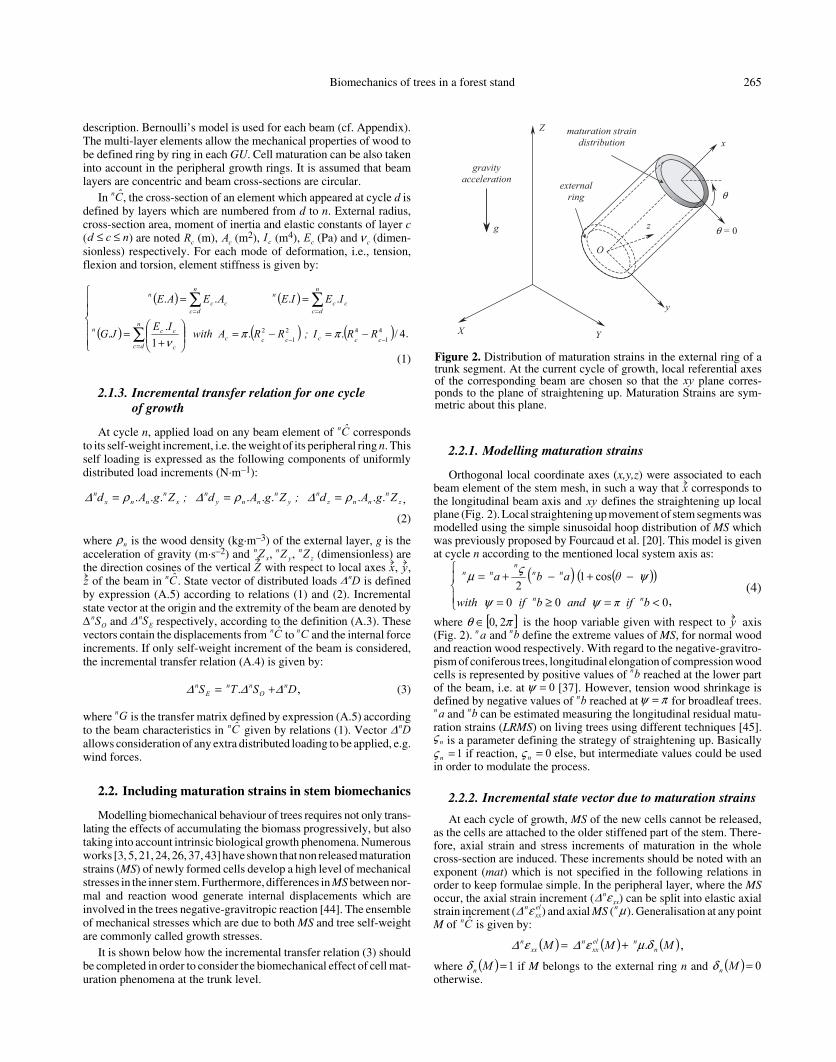
Orthogonal local coordinate axes (x,y,z) were associated to eachbeam element of the stem mesh, in such a way that corresponds tothe longitudinal beam axis and defines the straightening up localplane (Fig. 2). Local straightening up movement of stem segments wasmodelled using the simple sinusoidal hoop distribution of MS whichwas previously proposed by Fourcaud et al. [20]. This model is givenat cycle n according to the mentioned local system axis as:
(4)
where is the hoop variable given with respect to axis(Fig. 2). and define the extreme values of MS, for normal woodand reaction wood respectively. With regard to the negative-gravitro-pism of coniferous trees, longitudinal elongation of compression woodcells is represented by positive values of reached at the lower partof the beam, i.e. at [37]. However, tension wood shrinkage isdefined by negative values of reached at for broadleaf trees.
and can be estimated measuring the longitudinal residual matu-ration strains (LRMS) on living trees using different techniques [45].
is a parameter defining the strategy of straightening up. Basically if reaction, else, but intermediate values could be used
in order to modulate the process.
2.2.2. Incremental state vector due to maturation strains
At each cycle of growth, MS of the new cells cannot be released,as the cells are attached to the older stiffened part of the stem. There-fore, axial strain and stress increments of maturation in the wholecross-section are induced. These increments should be noted with anexponent (mat) which is not specified in the following relations inorder to keep formulae simple. In the peripheral layer, where the MSoccur, the axial strain increment ( ) can be split into elastic axialstrain increment ( ) and axial MS ( ). Generalisation at any pointM of is given by:
,
where if M belongs to the external ring n and otherwise.
Cn
ncd ≤≤ cR cA cI cE cν
( ) ( )
( ) ( ) ( )
−=−=
+
=
==
−−=
==
∑
∑∑
4/..1
..
....
41
421
2cccccc
n
dc c
ccn
n
dccc
nn
dccc
n
RRI ; RRA withIE
JG
IEIE AEAE
ππν
.
Cn
zn
nnzn
yn
nnyn
xn
nnxn ZgAd; ZgAd; ZgAd ......... ρ∆ρ∆ρ∆ ===
nρx
nZ ynZ z
nZZ x y
z Cn Dn∆
OnS∆ E
nS∆Cn Cn
DST S nO
nnE
n ∆∆∆ += .
Gn
Cn Dn∆
Figure 2. Distribution of maturation strains in the external ring of atrunk segment. At the current cycle of growth, local referential axesof the corresponding beam are chosen so that the plane corres-ponds to the plane of straightening up. Maturation Strains are sym-metric about this plane.
xy
xxy
( ) ( )( )
<=≥=
−+−+=
000
cos12
bπ if and b if with
θ a b a
nn
nnn
nn
ψψ
ψςµ
,
[ ]πθ 2,0 ∈ yan bn
bn
0=ψbn πψ =
an bn
nς n 1=ς n 0=ς
xxnε∆
elxx
nε∆ µnCn
( ) ( ) ( )M M M nnel
xxn
xxn δµε∆ε∆ .+=
( ) 1=Mnδ ( ) 0=Mnδ

266 P. Ancelin et al.
The symmetry assumption of MS distribution, with respect to the plane, allows the maturation effects to be restricted to the superpo-
sition of generalised strain increments of longitudinal tension ( )and bending around the axis ( ). Consequently, the total axialstrain increment at point M(x, y, z) can be written under the followingform:
.
Denoting E(M) the longitudinal Young’s modulus at point M (Pa), theaxial stress increment (Pa) at point M is given by:
(5)
This axial stress field is self balanced in any beam cross-section area, i.e., there are no internal forces due to the maturation [2]. It follows:
and . (6)
Generalised tensile and bending strain increments due to the matura-tion are deduced by substituting from relation (5) the longitudinalstress increment in (6). The orthogonal local coordinate axes (x,y,z)corresponding to inertia principal axes of the beam, it becomes:
, (7)
where is the cross section area of the peripheral ring n.Using the MS model (4) in integral equations (7), generalised strain
increments due to maturation can be expressed as:
By definition, the incremental state vector due to maturation containssix displacement components and six internal force increments. Thelatter are denoted as zero as maturation does not induce internal forces.Generalised displacement increments are obtained by integratingstrain compatibility equations of the Bernoulli’s model. We obtain:
.
Finally, incremental state vector due to maturation in is given fora beam of length L by:
.
For a beam submitted to both distributed load increment and peripheralmaturation strains, the incremental transfer relation (3) takes the fol-lowing form:
. (8)
2.3. Stages of the Incremental Transfer Matrix Method
In , tree trunk shape is discretized by n beam elements of length (i = 1… n) (m). These elements are connected together by structural
nodes numbered along the stem from the base to the top (i = 1… n+1).Convention states that element is on the left and element i is onthe right of node i. The ITMM uses the state vectors which are
expressed on the left and on the right of each node i of the structure(Fig. 3) by:
and . (9)
Components of and are expressed in the local coordinatesystem of elements and i, respectively. and containthe generalised displacements of node i whereas contains theforces which are transmitted by node i on element and con-tains the forces which are exerted by node i on element i. The ITMMallows increments of nodal displacements and internal forces to bedetermined during the cycle n.
2.3.1. Node equilibrium and element changing
Let be the 3 × 3 direction cosine matrix which is used to trans-form vector coordinates from element to the element i coordinatesystem. The vectors which contain the six generalised displacementincrements on the left and on the right of node i are linked by the matrixrelation:
with . (10)
Furthermore, let denote the vector of external force incrementsconcentrated at node i, e.g. crown weight or wind forces. The mechan-ical equilibrium at node i in the local coordinate system of element iis written as:
. (11)
According to relations (10) and (11), we infer incremental state vec-tor expression on the right of node i in step with its expression on the left:
, (12)
with and .
xyε∆ n
z znK∆
( ) znn
xxn Ky M ∆ε∆ε∆ .−=
( ) ( ) ( ) ( ) ( )( )M KyMEMMEM nn
znnel
xxn
xxn δµ∆ε∆ε∆σ∆ .... −−==
An
( )∫ =An
xxn dAM 0.σ∆ ( )∫ =
Anxx
n dAMy 0.. σ∆
( ) ( ) ∫∫−
==nA
nn
nz
n
nA
nn
nn dAyIE
EK; dA
AEE
...
..
µ∆µε∆
nA
( )( )
( )( )( )
−−−=
−+=
− ψςπ∆
ςε∆
cos..6
..
2..
31
3 RR a b IE
EK
a baAE
AE
nnnn
nn
n
zn
nnn
nn
nnn
xK ; xK v; x u zn
zn
znnnn .
2..
2
∆ω∆∆∆ε∆∆ ===
Cn
t
zn
znnn |LKLKLM 000000.000
2..
2
∆∆ε∆∆ =
MDST S nnO
nnE
n ∆∆∆∆ ++= .
Cn
iL
1−i
Lin
n
Lin
FQ
S,
,
=∆∆∆
Rin
n
Rin
FQ
S,
,
=∆∆∆
LinS ,∆ Ri
nS ,∆1−i Li
nQ ,∆ RinQ ,∆
LinF ,∆1−i Ri
nF ,∆
in B
1−i
Lin
in
Rin QK Q ,, .∆∆ =
=
×
×
in
in
in
BBK
33
33
00
inCL∆
in
Lin
in
Rin CLFK F ∆∆∆ +−= ,, .
in
Lin
in
Rin CSP S ∆∆∆ += ,, .
−
=×
×
in
in
in
KK
P66
66
00
=
ini
n
CLC
∆∆ 60
Figure 3. Functional scheme of the Incremental Transfer MatrixMethod (ITMM) applied on a growing tree trunk. The stem is discre-tized with beam elements which are connected to each other bynodes. The ITMM consists of determining the state vectors tracing thestructure node by node. Considering element i, state vector of thebeam origin (node i) is determined using the equilibrium equationwith the previous adjacent element . State vector of the extremitynode is calculated using the transfer relation on element i.
1−i1+i
.
Biomechanics of trees in a forest stand 267
2.3.2. Incremental transfer on element
The matrix relation, which allows the incremental state vector onthe left of node to be expressed according to the incremental statevector on the right of node i, is directly inferred from relation (8) andwritten as:
, (13)
where , and are given by , and expressionsusing self characteristics of element i.
2.4. Incremental application of crown weight on stem structure
Most of the static loads which are applied on a tree are due to thecrown biomass increments resulting from addition and loss ofbranches. As the crown structure of simplified trees is not explicitlyknown, the weight increment distribution along the stem uses anempirical form, which can depend on the tree species. The notationsused in order to detail the application of crown weight increment ontree stem are set out in Table I.
2.4.1. Global balance of crown biomass increment at cycle n
At cycle n, the global tree crown biomass increment is formallygiven by the difference between the current and the previous totalweight of the crown: . This weight incrementalso results from the balance between the positive increment of new
vegetative biomass provided from growth and the negative incrementensuing from branch loss, so that: . Loss ofcrown biomass is assumed to be mainly due to pruning of lowestbranches. The stem can therefore be split into three zones:
where the positive weight increment is distributed;where the negative weight due to loss of biomass is
applied; , not directly loaded by the crown weight.
2.4.2. General procedure for applying crown weight increment
Distribution of crown weight increment along the stem is given atcycle n by the discontinuous function with regardto the following procedures:
– The negative increment of weight is calculated at height considering the local total biomass which has been removed betweencycles n–1 and n. This local weight is explicitly determined by thecumulative formula:
.
– The total loss of biomass due to pruning in the region induces
a reduction of weight which is given by: .
– The addition of weight due to the crown growth is given by. This weight is distributed along the zone
using an analytical function which must fulfil the followingcondition:
. (14)
Note that .Function is related to the crown biomass balance between twoconsecutive cycles of growth. This function is therefore associatedwith crown architecture and gives the spatial and temporal distributionof biomass, as well as the local vigour of growth. It is not easy to esti-mate with regard to the global crown shape only. This functionhas to be determined empirically for each species of interest. An alter-native is to use architectural models, such as those developed byAMAP [34, 35], which allow the structural variability to be considered.
In practice, function is given as a discrete form and repre-sents concentrated forces which are applied at stem nodes . Theresulting vector of nodal forces is thus incorporatedinto equation (11). Condition (14) becomes:
. (15)
Moreover, these concentrated forces define an approximation of realloads whereas branch topology and mass distribution in the crown arenot given explicitly.
2.5. Final ways to achieve the biomechanical analysis of tree stem
2.5.1. Particular procedures related to stem growth
The numerical developments and subsequent simulations weremainly concerned by secondary biomechanical processes due to celldifferentiation. For this reason, the influence of apical reorientation isnot discussed here, even if this phenomenon can be strongly involvedin tree stem movement and defects [18, 19, 44]. We will therefore
Table I. Summary of notations used to apply crown weight incre-ments on tree stem.
Notationa Unit Definition
kg Global crown weight increment
kg Total weight of the crown
kg Positive crown weight increment due to growth
kg Negative crown weight increment due to pruning
m Total tree height
m Crown base height
— Current crown zone on the stem
— Intermediate pruned zone
— Stem zone without branches
— Number of stem nodes in the crown(in )
m Height in the tree
kg·m–1 Discontinuous distribution of crown wei-ght increment
kg·m–1 Distribution of crown weight increment due to growth
kg Discrete form of for nodes i of
a The n exponent means that notations are used at cycle of growth n.
CWIn
CWTn
+CWIn
−CWIn
Hn
CBHn
[ ]HCBHCZ nnn ,=
[ ]CBHCBHPZ nnn ,1−=
[ ]CBHSZ nn 1,0 −=
CNn
CZn
[ ]Hh n,0∈
( ) [ ]Hh hW nn ,0, ∈∆
( ) CZ h hw nn ∈,
in w ( )hwn CZn
1+i
in
in
Rin
in
Lin MDST S ∆∆∆∆ ++=+ ,,1 .
inT i
nD∆ inM∆ Tn Dn∆ Mn∆
CWTCWTCWI nnn 1−−=
−+ += CWICWICWI nnn
CZn +CWIn
PZn −CWIn
SZn
( ) [ ]HhhW nn ,0, ∈∆
PZ h n∈
( ) ( )∑−
=
−=1
1
n
i
in hWhW ∆∆
PZn
( )∫ ∑
−=−
=
−
PZn
n
i
in dhhWCWI1
1
∆
−+ −= CWICWICWI nnn CZn
( )hwn
( ) =∫ dhhwCZn
n . +CWIn
CWIn + ≥ CWIn
( )hwn
( )hwn
( )hwn
CZi n∈( )in
in wfCL =∆
∈
=∑ wCZn i
in +CWIn

268 P. Ancelin et al.
consider that the new apical GU is formed in the same direction of thebearing element.
The secondary straightening up is induced by a differential of mat-uration strains in the plane of flexion which is due to the presence ofreaction wood. Stimuli of reaction wood formation are not well-known. However, the secondary reorientation criterion can be givenas a function of the stem leaning angle [1, 37, 42, 44, 46]. It can alsobe dependent on other variables, such as the stress (or strain) field forinstance [11]. The geometrical criterion which was used in softwareAMAPpara [20] was chosen to control the negative-gravitropism inour model. A threshold angle (with respect to the vertical direction)was used once to indicate the beginning of the stem straightening up.Moreover, a second threshold angle was defined to control thestraightening up of each GU. The reorientation process was simulatedat each cycle n according to the following algorithm: from the begin-ning of tree growth, we have in the law (4) for every GU, i.e.the stem cannot react; during cycles of growth, if the leaning angle ofone GU at least is greater than then the trunk starts to react; then foreach GU, a reaction occurs ( ) if its leaning angle is greater than
and there is no reaction otherwise ( ). Note that the thresholdangle , which is the same for every GU, can be defined for each cycleof growth, e.g. to be assimilated to the Gravitropic Set-point Angledefined by Digby and Firn [15]. Nevertheless, it will be assumed con-stant during growth in the results section: . Moreover, as men-tioned above, intermediate values of could be used in order to mod-ulate the straightening up intensity. This parameter could be particularlygiven as a function of the leaning angle allowing the correlationbetween negative-gravitropism intensity and stem inclination to betaken into account [42, 44, 46].
2.5.2. Starting of the stem analysis method
Each trunk is considered as a tapered cantilever. It is assumed tobe perfectly embedded in the soil with a free extremity. The 12 asso-ciated boundary conditions (BC) are given by:
(16)
Six components of incremental state vectors at the right of node 1 andsix components at the left of node are determined by these con-ditions. The Transfer Matrix Method consists of finding a linear sys-tem allowing the six unknown components of each vector to be solved.Going stepwise from the first till the last node, and using successivelythe transfer relations (13) and (12), allows this system to be estab-lished. After operating all matrix products and using BC (16), it cantake the following symbolic form:
.
This system allows the boundary state vectors to be completelyknown. In particular, the reaction forces at the fixed base are:
. From , the stepwise procedure mentionedabove allows the incremental state vector to be determined at all nodesof the structure. This process is the general method and leads a startingpoint for isostatic or hyperstatic problems. For a cantilever problem,it is easier to determine the reaction forces at the embedded base byexpressing the global trunk equilibrium, i.e. calculating the resultingforces and moments due to external loading.
2.5.3. Outputs of the trunk biomechanical model
The increments of nodal displacements are computed in a localcoordinate system, crossing step by step beam elements of trunk withrelations (12) and (13). After transforming these displacements in theglobal coordinate axes, the new stem shape, which corresponds to thenew configuration , is determined. At each cycle, the location ofreaction wood sectors in the current ring is saved. A post treatmentallows cartographies of normal and reaction wood to be mapped atchosen positions along the stem. Furthermore, our model providesinternal growth stresses which are linked with the current stem shape.Increment of stress is determined by computing generalised strainincrement and using the material behaviour law of each wood layer,according to equation (5). The total field of stresses (Pa) depends onthe growth and loading history according to the cumulative relation[19]:
,
where is the apparition cycle of the layer c of beam element i.
2.6. Evaluation of the simplified tree model
2.6.1. Description of reference trees
Simulations of tree growth were performed with the softwareAMAPpara and its biomechanical function AMAPméca. The com-puted structure was taken as a reference in order to carry out a numer-ical evaluation of the ITMM biomechanical model. The advantage ofthis approach was to control both structural and mechanical parame-ters used for the calculations.
The reference tree corresponded to a model of Maritime pine (Pinuspinaster Ait.) which was already used by Fourcaud et al. [20]. Stemwood was considered to be homogeneous and isotropic. Young mod-ulus E was equal to 11 GPa in all the rings and wood density ρ wasequal to 700 kg·m–3. The maturation strain model (4) was used with
for normal wood and for compression wood.These values were in good agreement with those measured by Alteyracet al. [1] on a 17 year-old Maritime pine. The stem was considered tohave an initial leaning angle of 30°. The computed distribution of crownbiomass increments was recorded at each step of calculation. Threestrategies of biomechanical behaviour were considered (Fig. 4). TreeT1 was computed without a negative-gravitropic response, i.e. taking
in equation (4). This extreme case is of course not realistic but
α
βn
0=ςn
α1=ςn
βn 0=ςnβn
ββ =n
ςn
top eerf ta BC mechanical
base ixedf ta BC lgeometrica
F
Q
Lnn
Rn
6
6
0
0
,1
,1
⇒
⇒
=
=
+∆
∆.
1+n
+
=
+
Fn
Qn
Rn
FFn
FQn
QFn
QQn
Lnn
BB
FAAAAQ
,1
,1 0.
0 ∆∆
Fn
FFn
Rn BA F .1
,1−−=∆ R
nS ,1∆
Cn
∑=
=n
icd d
icd
icn
,
,, σ∆σ
icd ,
Figure 4. Reference trees have been computed with the softwareAMAPpara. Different final shapes were obtained using three strate-gies of straightening up. Tree T1 was performed without consideringsecondary straightening up, whereas trees T2 and T3 were submittedto maturation stresses inducing a stem negative-gravitropism.Results are shown at 20th cycle of growth.
% a 02.0−= % b 1.0=
0=ςn

Biomechanics of trees in a forest stand 269
it allows several models of crown mass distribution to be evaluatedwithout any other influencing parameters. Secondary reorientationprocesses of trees T2 and T3 were controlled with threshold parameters
and respectively, according tothe straightening up strategy described in the previous section. In allthe simulations, a new GU was placed in the prolongation of the stemtip, i.e. primary reorientation was not considered.
2.6.2. Loading functions for crown weight increments
The ITMM was tested taking into consideration the biomass incre-ments of the reference tree at each cycle of growth. Crown incrementof mass and stem growth parameters (GU length and ring width) weretaken from AMAPpara at each step. The crown biomass was givenunder a natural discrete form at each stem whorl. In the calculations,stem discretization was achieved so that generated nodes coincidedwith the whorl set and were numbered from the stem base to the tip.At cycle n, the number of stem nodes, including the embedded trunkbase, is thus n+1 and the number of whorls bearing living branches isdenoted . Crown weight increments were applied considering thefollowing functions of weight distribution (Fig. 5):
– Single concentrated load (SC): the crown weight increment can be condensed as a single resultant force which occurs to the centreof crown mass increments. Positive and negative increments and are not used in that case. It is assumed that this centre ofmass is located at a node of the stem line which is given by AMAP-para. This hypothesis allows the load to be applied at a relative locationwith regard to the current deformed structure. This choice is necessaryto compare ITMM results with AMAPméca calculations as the inter-mediate reference configurations are not identical (cf. Fig. 6 forinstance). The loading due to crown weight is therefore determinedby = . This aggregated model has been considered becauseof its simplicity. This is indeed the first model which comes to mindfor applications at the stand scale.
– Real load distribution per whorl (RW): crown weight increment is distributed in accordance with the real distribution of branch
biomass which is explicitly given by AMAPpara for each stem whorl.This distribution includes negative values which are applied to the
( ) ( )°°= 04522 ,,βα ( ) ( )°°= 103533 ,,βα
Figure 5. Distributions of crown biomassincrements along the stem. DU: discreteuniform distribution. DL: discrete lineardistribution. DSR: discrete square root dis-tribution. DQ: discrete quadratic distribu-tion.
CNn
CWIn
+CWIn
−CWIn
cN
wcn CWIn
Figure 6. Stem shape resulting from 20 calculation steps of tree T1using different distribution modes of crown biomass increments inthe ITMM procedure. RW: real distribution per whorl. SC: single con-centrated load. DU: discrete uniform distribution. DL: discrete lineardistribution. DSR: discrete square root distribution. DQ: discrete qua-dratic distribution.
CWIn

270 P. Ancelin et al.
pruned whorls. Positive and negative increments and are not directly used in this case. Nevertheless they can be deducedsumming the contribution of each whorl.
– Discrete uniform load distribution (DU): the function of weight
distribution is given by for all nodes . Condition (15)
gives .
– Discrete linear load distribution (DL): the function of weight dis-
tribution is given by , . Condition (15)
gives .
– Discrete square root load distribution (DSR): the function of
weight distribution is given by , , giving
.
– Discrete quadratic load distribution (DQ): the function of weight
distribution is given by , , giving
.
3. RESULTS AND DISCUSSION
3.1. ITMM validation for a non-branching growing stem
Numerical validation of our biomechanical model has beenachieved by comparing the results of calculations obtained withAMAPméca for a reference growing stem without branches.Two cases were studied: firstly, loading due to the stem self-weight was only considered, and secondly, the negative-grav-itropic response due to differential maturation strains was takeninto account. In both cases, the computed displacement incre-ments and cumulated growth stresses inside the stem were iden-tical between the two models. The ITMM based biomechanicalmodule has thus been correctly formulated and implemented,and it is therefore considered numerically validated. Withregard to the finite element method, the computation methodused does not involve differences in the calculated stemresponse.
3.2. Evaluation of the simplified tree model
The model presented in this paper and the module AMAP-méca share the same biomechanical assumptions: the use of ahomogeneous and isotropic material for stem wood, thedescription of stem internal structure using multi-layer 3Dstraight beam elements with circular cross-sections and con-centric layers, the sinusoidal hoop distribution of maturationstrains in the peripheral wood ring and the geometrical strategyof the negative-gravitropic response using two constant thresh-old angles, are common for the two models. Hence, as theITMM provided the same results for non-branching stems as
those obtained with the finite element method used in AMAP-méca, the only difference between our biomechanical modeland AMAPméca is the crown description. This description wassimplified and aggregated here, while AMAPpara allows bio-mechanical calculations to be achieved using architectural treestructures. As shown above, our ITMM based model uses the-oretical discrete distributions of concentrated loads allowingthe application of crown weight on the tree stem.
3.2.1. Model evaluation without secondary straightening up
First results were obtained using AMAPpara reference treeT1, i.e. without taking into consideration secondary straighten-ing up (Fig. 6). At a given stage, stem shape results from a step-wise calculation during which increments of weight wereapplied progressively. However, as already explained by Four-caud et al. [20], large resulting curvature is not due to stem flex-ibility but originates from a geometrical effect as the primarygrowth occurred at each cycle on a deformed shape. In the fol-lowing discussions, it should be kept in mind that shape diver-gence which could be noted at a given stage resulted fromcumulated differences during the stepwise calculation.
The ITMM result using loading RW does not show as goodaccuracy as was expected. This can be explained by the fact thatbranch weights were resumed to resultant forces applied tostem whorls, neglecting residual moments which were alsotransmitted to the trunk. SC loading led to a solution which wasmuch straighter than the reference stem bending. Weight repar-tition along the stem was not taken into account and explainsa part of this difference. Moreover, resultant moments werealso neglected due to the hypothesis that the centres of massincrements were placed on the stem line. For large deflections,this assumption becomes not valid and the crown weight effecttends to be underestimated.
In view of the repartition of biomass increments (Fig. 5), itis clear that the best results (Fig. 6) were obtained with modelsfitting well the reference biomass at the top part of the crown.Loading model DL led on the best approximation at 20 cyclesfor instance. On the contrary, DU and DSR gave non-satisfac-tory responses even if they fitted well the biomass distributionat the crown base. This statement is not surprising as beam stiff-ness decreases significantly from the base to the tip accordingto the stem taper. Moreover it is well-known that cantileverbeam deflection is more sensitive to loads which are appliednear the free extremity.
3.2.2. Model evaluation with negative-gravitropic response
Reference trees T2 and T3 (Fig. 4), which are associated withtwo different strategies of secondary straightening up, wereused to evaluate the ITMM in more realistic situations. Trunkshape evolution shows that basal curvature is initiated at thefirst stages of growth. During this period, the stem fine extrem-ity bends gradually under action of branch weight acting closeto the tip. Primary lengthening, which is achieved in the pro-longation of the stem, tends to amplify this deformation. Duringthe following cycles, secondary growth increases beam stiff-ness, reducing significantly movements of the basal part of the
+CWIn −CWIn
win = 0an CZi n∈
10 −=
+
CNCWIa n
nn
= win ( )1.1 +− inan CZi n∈
∑=
+
=CNn
k
nn
k
CWIa
1
1
= win ( )1.2 +− inan CZi n∈
∑=
+
=CNn
k
nn
k
CWIa
1
2
= win ( )23 1. +− inan CZi n∈
∑=
+
=CNn
k
nn
k
CWIa
1
23
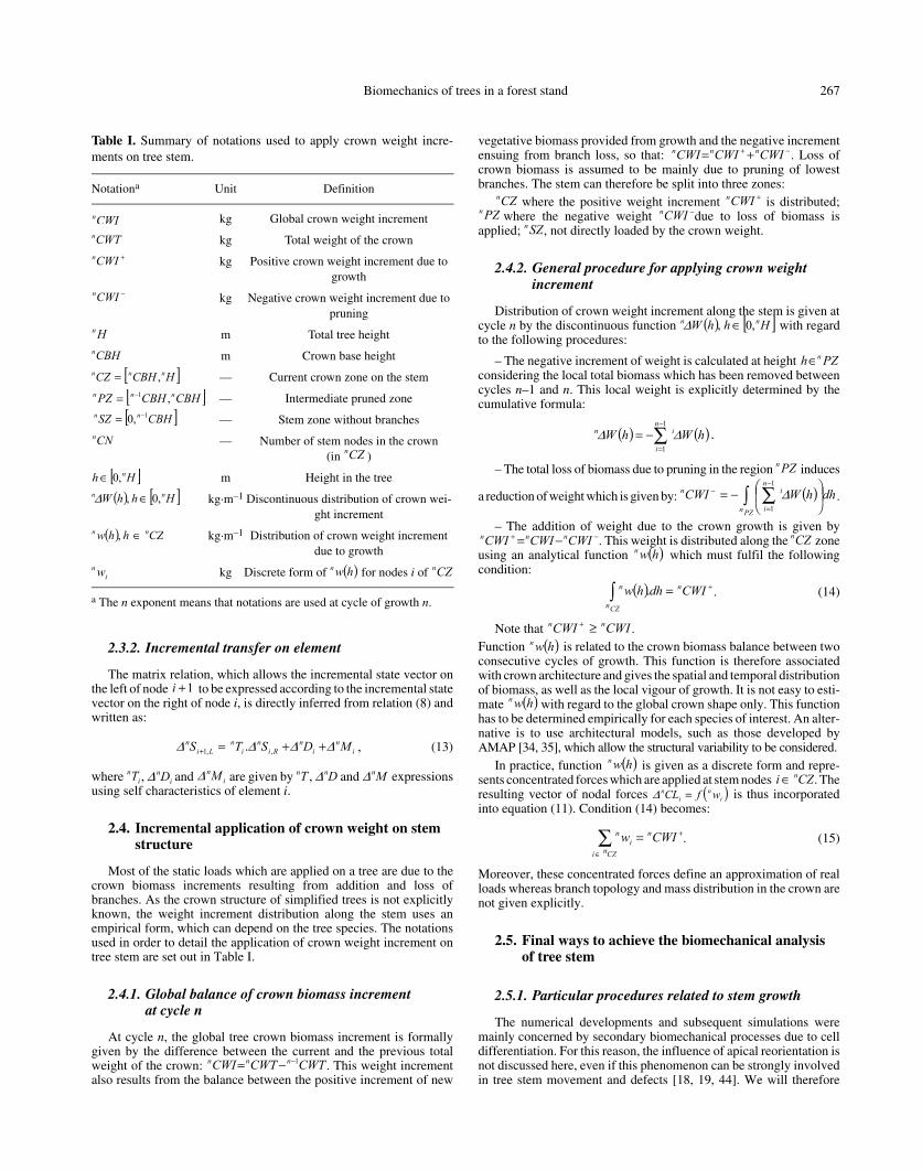
Biomechanics of trees in a forest stand 271
trunk. Inversion of stem curvature appears when the leaningangle of young terminal GUs reaches the stem straightening upthreshold . The tree apex then tends to return to a vertical posi-tion. Maximum stem curvatures, from which location thusdepend generally on this angle , are situated at half stemheight for tree T2 and one third of trunk height for tree T3.
Only crown loading models SC, RW and DL were appliedin order to test ITMM, as other distributions were shown not tobe satisfying. Fairly good agreements can be seen in the lowertwo thirds of the trunk for both strategies T2 and T3 (Fig. 7).In each case, the three ITMM calculations reach a maximumcurvature at the same location on the trunk, except for SCapplied on tree T2. Radii of curvature are also very close in eachtest. Nevertheless, results are globally better for tree T3 forwhich the model DL is very good. These responses can beexplained by looking at the previous results relative to tree T1.Models SC and RW, underestimating the real bending, reach thethreshold of straightening up later than the reference tree,whereas model DL, which overestimates this bending, starts toreact earlier. Consequently, delay or advance of the reactionprocess involves divergence of mechanical response. It can alsobe noticed that the sooner stem verticality is reached the lessvisible the differences between models. Stem closeness fromthe vertical position indeed limits bending moments which aregenerally responsible for the recorded shape differences.
Model evaluation was also concerned with the calculationof longitudinal growth stresses (LGS). These stresses werecomputed for both trees T2 and T3 using the ITMM and con-sidering crown loading models SC and DL. Results were com-pared with those obtained by AMAPméca. Good agreementswere found concerning the LGS general radial profiles in thepart of the stem which is situated below the straightening upzone, i.e. under the maximum curvature (Fig. 8). Nevertheless,maximum tensile LGS at the stem base is not always located at
the same distance of the pith and their intensity is significantlydifferent for tree T3. These gaps can be explained by the delayor advance of the reaction processes. Differences of stressintensity can also result from the different positions of the upperpart of the stem (Fig. 7) which involve different bendingmoments due to the crown weight. Basal growth units showmore LGS divergence as they have a longer growth history andthus support more stress increments. For the same reason, dif-ferences can also be visible in the more internal growth rings.LGS profiles are not comparable in cross-sections closed to thezone of maximum curvature. No more accordance of LGS dis-tribution is observed in cross sections in the upper part of thestem. Leaving radial distribution out of account and consider-ing only the maximum and minimum LGS values, it is inter-esting to notice the strong accordance of the results for tree T2(Fig. 9) as well as in the first half of tree T3.
4. CONCLUSION
The ITMM is a simple and efficient method to simulate thebiomechanical behaviour of growing trees. Nevertheless, theuse of numerical methods at the forest stand scale, i.e. on a largenumber of trees, necessitates representing the influence of thecrown weight using an aggregated form. It was shown that thissimplification is not trivial. At each cycle of growth, locationof newly appeared biomass as well as position of lost materialinto the crown is highly species dependent. Furthermore, thestem negative-gravitropism can significantly modify the valid-ity of load application models, giving more or less acceptableresults in terms of stem shape or inner LGS. Quality of calcu-lation outputs depends on criteria that are used for applicationsat the stand scale. In order to characterise timber quality inAquitaine maritime pine forests for instance, foresters oftenlook at the stem base leaning and intensity of the basal curvaturewhich provide good indicators of pith eccentricity and theamount of compression wood. On the other hand, growthstresses in broadleaf trees are often considered as the mostimportant factor responsible for log end-splitting or criticalsawn board distortions. Evaluation of models with regard to theexpected output for specific applications is therefore of greatinterest. It has been shown that severe simplifications of crownloading can provide relatively good agreements in terms of bothshape and LGS distribution, at least in the valuable part of thetrunk. Architectural models allow typical tree structures to begenerated. These virtual trees would be useful to determinemore adapted models of biomass repartition, to be used on sim-plified trees at the stand scale for a given purpose.
The objective of future studies will be to perform numericalanalyses of stem shape variability and wood quality, taking intoconsideration environmental constraints, i.e. spatial competi-tion or the silvicultural scenario used. For this purpose, theITMM will be coupled with spatial competition models devel-oped in CAPSIS.
Acknowledgements: This work was carried out during a PhD thesiswhich was funded by INRA-FMN and Région Aquitaine. We wish tothank Alexia Stokes and Neal Harries for their corrections andlanguage review. We also thank two anonymous reviewers for theircomments and suggestions.
α
α
Figure 7. Stem shape resulting from 20 calculation steps of A/ treeT2 and B/ tree T3 using different distribution modes of crown bio-mass increments in the ITMM procedure. RW: real distribution perwhorl. SC: single concentrated load. DL: discrete linear distribution.

272 P. Ancelin et al.
APPENDIX: BASICS OF THE TRANSFER MATRIX METHOD OF 3D STRAIGHT BEAMS
A full description of the strength of materials, including elas-ticity and beam theories, is given by Timoshenko [38]. TheTransfer Matrix Method is described by Tuma [40] and its for-mulation with 3D straight beams is detailed by Ancelin [2].
A1. Kinematics
3D straight beam is characterised by associated vectors ofgeneralised displacements ( , , , , , ) and generalisedinternal forces ( , , , , , ), according to the beamlocal reference axes , , (Fig. 10). Euler-Bernoulli assump-tions in beam theory give how a beam cross section rotates.Defining normals as the lines perpendicular to the beam’s
Figure 8. Radial distribution of longitudi-nal growth stresses in the plane of leaning,resulting from 20 steps of calculation andusing two distribution modes of crownbiomass increments in the ITMM proce-dure. SC: single concentrated load. DL:discrete linear distribution. Location ofgrowth units along the stem of trees T2and T3 is shown in Figure 7.
u v w xω yω zωxN yV zV xM yM zM
x y z

Biomechanics of trees in a forest stand 273
neutral fibre, assumptions stipulate these normals remain straight,unstretched and normal.
A2. Equilibrium
Equilibrium equations of the Static Fundamental Principledefine generalised internal forces according to uniformly dis-tributed loads , , :
. (A.1)
By using strain compatibility of Bernoulli’s model, weobtain the equations which define generalised displacementsaccording to generalised internal forces:
(A.2)
where E is the Young’s modulus and the shearmodulus, being Poisson’s coefficient. The moments of inertiaof the cross-section are defined with respect to the beam localreference axes , , by:
, where A isthe beam cross-section area.
A3. Transfer matrix method
We consider a 3D beam of length L with a circular cross-section. Moments of inertia of this cross-section verify
and . By integrating equations (A.1) and (A.2)between extremity nodes and , we obtain general-ised internal forces and generalised displacements at the beamnodes. State vectors at the beam origin and at the beamextremity are defined by:
(A.3)
The transfer relation links to and is written [2]:
, (A.4)
where T is the transfer matrix of the beam and D is the statevector of distributed loads. T and D matrices are given by:
; (A.5)
Figure 9. Maximal and minimal longitudi-nal growth stresses (LGS) along the stemfor A/ tree T2 and B/ tree T3. Results obtai-ned from 20 steps of calculation using twodistribution modes of crown biomass incre-ments in the ITMM procedure. SC: singleconcentrated load. DL: discrete linear dis-tribution.
Figure 10. Generalised displacements and internal forcesin a 3D straight beam subjected to distributed loads. , ,are the local reference axes of the beam. , , are the posi-tive translations of cross-section centre (m); , , arethe positive rotations of cross-section normal (radians). ,
, are the distributed loads (N·m–1), and are positive inthe local directions. (normal force, N), , (shear for-ces, N), (torsion moment, N.m), , (bendingmoments, N.m) are the positive internal forces.
x y zu v w
xω yω zωxd
yd zdxN yV zV
xM yM zM
xd yd zd
zz
yy
xx ; d
dxdV
; ddx
dV; d
dxdN
−=−=−=
yz
zyx V
dxdM
; Vdx
dM;
dxdM
−=== 0
yyx ;
dxdw;
dxdv;
AEN
dxdu
.−=== ωω
z
zz
y
yyxx
IEM
dxd
; IE
Mdx
d;
JGM
dxd
...===
ωωω ,
( )ν+= 12/EGν
y z x( )∫∫∫ +=== zy dAzyJ; dAyI; dAzI ... 2222
III zy == IJ 2=0=x Lx =
OS ES
=
−−−−−−=t
zEyExEzEyExEzEyExEEEEE
t
zOyOxOzOyOxOzOyOxOOOOO
M M M V V N | w v uS
M M M V V N | w v uS
ωωω
ωωω
.
ES OS
DSTS OE += .
TTTT
T
=
2221
1211 2
1
=
DD
D

274 P. Ancelin et al.
where:
;
;
;
;
REFERENCES
[1] Alteyrac J., Fourcaud T., Castera P., Stokes A., Analysis and simu-lation of stem righting movements in Maritime pine (Pinus pinasterAit.), in: Proc. Connection between silviculture and wood qualitythrough modelling approaches and simulation software, ThirdWorkshop of IUFRO WP S5.01-04, La Londe-Les-Maures, France,September 5–12, 1999, pp. 105–112.
[2] Ancelin P., Modélisation du comportement biomécanique de l’arbredans son environnement forestier. Application au pin maritime,Thèse de Doctorat, Université de Bordeaux I, France, N° 2343, 2001,182 p.
[3] Archer R.R., Growth Stresses and Strains in Trees, Springer VerlagSeries in Wood Science, Timell T.E. (Ed.), 1986.
[4] Biging G.S., Dobbertin M., Evaluation of competition indices inindividual tree growth models, Forest Sci. 41 (1995) 360–377.
[5] Boyd J.D., Compression wood: force generation and functionalmechanics, New Zeal. J. Forest Sci. 3 (1973) 240–258.
[6] Cannell M.G.R., Morgan J., Murray M.B., Diameters and dryweights of tree shoots: effect of Young's modulus, taper, deflectionand angle, Tree Physiol. 4 (1988) 219–231.
[7] Castéra P., Morlier V., Growth patterns and bending mechanics ofbranches, Trees-Struct. Funct. 5 (1991) 232–238.
[8] Cescatti A., Modelling the radiative transfer in discontinuous can-opies of asymmetric crowns. I. Model structure and algorithms,Ecol. Model. 101 (1997) 263–274.
[9] Cluzeau C., Dupouey J.L., Courbaud B., Polyhedral representationof crown shape. A geometric tool for growth modelling, Ann. Sci.Forest. 52 (1995) 297–306.
[10] Coligny (de) F., Ancelin P., Cornu G., Courbaud B., Dreyfus P.,Goreaud F., Gourlet-Fleury S., Meredieu C., Saint-André L., CAP-SIS: Computer-Aided Projection for Strategies in Silviculture:advantages of a shared forest-modelling platform, in: Amaro A.,Reed D., Soares P. (Eds.), Modelling Forest Systems, CABI Pub-lishing, Wallingford, UK, 2003, pp. 319–323.
[11] Constant T., Ancelin P., Fourcaud T., Fournier M., Jaeger M., TheFrench project SICRODEF: a chain of simulators from the treegrowth to the distortion of boards due to the release of growthstresses during sawing: First results, in: Proc. Connection betweensilviculture and wood quality through modelling approaches andsimulation software, Third Workshop of IUFRO WP S5.01-04, LaLonde-Les-Maures, France, September 5–12, 1999, pp. 377–386.
[12] Courbaud B., Goreaud F., Dreyfus P., Bonnet F.R., Evaluating thin-ning strategies using a Tree Distance Dependent Growth Model:some examples based on the CAPSIS software “Uneven-AgedSpruce Forests” module, For. Ecol. Manag. 145 (2001) 15–28.
[13] Courbaud B., Coligny (de) F., Cordonnier T., Simulating radiationdistribution in a heterogeneous Norway spruce forest on a slope.Agric. For. Meteorol. 116 (2003) 1–18.
[14] Courbet F., Houllier F., Modelling the profile and internal structureof tree stem. Application to Cedrus atlantica Manetti, Ann. For. Sci.59 (2002) 63–80.
[15] Digby J., Firn R.D., The gravitropic set-point angle (GSA): the iden-tification of an important developmental controlled variable govern-ing plant architecture, Plant Cell Environ. 59 (1995) 1434–1440.
[16] Dreyfus P., Bonnet F.R., CAPSIS (Computer-Aided Projection ofStrategies in Silviculture): an interactive simulation and comparisontool for tree and stand growth, silvicultural treatments and timberassortment, in: Proc. Connection between silviculture and woodquality through modelling approaches and simulation software.IUFRO WP S5.01-04 second workshop, Berg-en-Dal, KrugerNational Park, South Africa, August 26–31, 1996, pp. 57–58.
[17] Ford E.D., Sorrensen K.A., Theory and models of inter-plant com-petition as a spatial process, in: DeAngelis D.L., Gross L. (Eds.), Pop-ulations, Communities and Ecosystems, Individual-Based Modelsand Approaches in Ecology, Chapman & Hall, New York, 1992,pp. 363–407.
[18] Fourcaud T., Défauts de forme et structure interne du Pin maritime,in: Actes du 5e colloque “De la forêt cultivée à l’industrie de demain– Propriétés et usages du Pin maritime”, ARBORA, 2–3 décembre,Bordeaux, France, 1999, pp. 77–84.
[19] Fourcaud T., Lac P., Numerical modelling of shape regulation andgrowth stresses in trees. Part I: an incremental static finite elementformulation, Trees-Struct. Funct. 17 (2003) 23–30.
−=
10000001000000100000100
00010000001
11L
L
T
−
−−
−
−
−
=
EIL
EIL
EIL
EIL
GJL
EIL
EIL
EIL
EIL
EAL
T
0002
0
002
00
00000
02
06
00
2000
60
00000
2
2
23
23
12
=
000000000000000000000000000000000000
21T
−−−
−−
−−
=
1000001000001000000100000010000001
22
LL
T
t
yzzyx
EIdL
EIdL
EIdL
EIdL
EAdL
D66
024242
33442
1−−
=
t
yzzyx
dLdLLdLdLdD
220
22
2−
−−−= .

Biomechanics of trees in a forest stand 275
[20] Fourcaud T., Blaise F., Lac P., Castéra P., Reffye (de) P., Numericalmodelling of shape regulation and growth stresses in trees. Part II:implementation in the AMAPPARA software and simulation of treegrowth, Trees-Struct. Funct. 17 (2003) 31–39.
[21] Fournier M., Bordonne P.A., Guitard D., Okuyama T., Growth stresspatterns in tree stems – A model assuming evolution with the treeage of maturation strains, Wood Sci. Technol. 24 (1990) 131–142.
[22] Fournier M., Baillères H., Chanson B., Tree biomechanics: growth,cumulative prestresses, and reorientations, Biomimetics 2 (1994)229–251.
[23] Gardiner B., Peltola H, Kellomäki S., Comparison of two models forpredicting the critical wind speeds required to damage coniferoustrees, Ecol. Model. 129 (2000) 1–23.
[24] Gillis P.P., Theory of growth stresses, Holzforschung 27 (1973)197–207.
[25] Hallé F., Oldemann R.A.A., Tomlinson P.B., Tropical trees and for-ests, Springer Verlag, Berlin, 1978.
[26] Kubler H., Growth Stresses in Trees and Related Wood Properties,For. Abs. 48 (1987) 130–189.
[27] Lemoine B., Growth and yield of maritime pine (Pinus pinasterAit.): the average dominant tree of the stand, Ann. Sci. Forest. 48(1991) 593–611.
[28] Milne R., Blackburn P., The elasticity and vertical distribution ofstress within stems of Picea sitchensis, Tree Physiol. 5 (1989) 195–205.
[29] Morgan J., Cannell M.G.R., Structural analysis of tree trunks andbranches: tapered cantilever beams subject to large deflections undercomplex loadings, Tree Physiol. 3 (1987) 365–374.
[30] Morgan J., Cannell M.G.R., Support cost of different branchdesigns: effects of position, number, angle and deflection of laterals,Tree Physiol. 4 (1988) 303–313.
[31] Morgan J., Cannell M.G.R., Shape of tree stems – a re-examinationof the uniform stress hypothesis, Tree Physiol. 14 (1994) 49–62.
[32] Peltola H., Nykänen M.L., Kellomäki S., Model computations on thecritical combination of snow loading and wind speed for snow dam-age of Scots pine, Norway spruce and Birch sp. at stand edge, For.Ecol. Manage. 95 (1997) 229–241.
[33] Pukkala T., Methods to describe the competition process in a treestand, Scand. J. For. Res. 4 (1989) 187–202.
[34] Reffye (de) P., Fourcaud T., Blaise F., Barthélémy D., Houllier F.,A functional model of tree growth and tree architecture, Silva Fenn.31 (1997) 297–311.
[35] Reffye (de) P., Houllier F., Blaise F., Fourcaud T., Essai sur les rela-tions entre l’architecture d’un arbre et la grosseur de ses axes végéta-tifs, in: Modélisation et Simulation de l’architecture des végétaux,INRA Ed., Sciences Update, 1997, pp. 255–423.
[36] Sorrensen-Cothern K.A., Ford E.D., Sprugel D.G., A model of com-petition incorporating plasticity through modular foliage and crowndevelopment, Ecol. Monogr. 63 (1993) 277–304.
[37] Timell T.E., Compression Wood in Gymnosperms, Springer Seriesin Wood Science, Springer-Verlag, Berlin, 3 vol., 1986.
[38] Timoshenko S.P., Résistance des matériaux, Dunod ed., Paris (trans-lated from: Strength of materials, D. Van Nostrand Company Inc.,Princeton), 1968.
[39] Tomé M., Burkhart H.E., Distance-dependent competition measuresfor predicting growth of individual trees, For. Sci. 35 (1989) 816–831.
[40] Tuma J.J., Structural analysis, McGraw-Hill, 1968.
[41] West P.W., Jackett D.R., Sykes S.J., Stresses in, and the shape of,tree stems in forest monoculture, J. Theor. Biol. 140 (1989) 327–343.
[42] Wilson B.F., Gartner B., Lean in red alder (Alnus rubra): growthstress, tension wood and righting response, Can. J. For. Res. 26(1996) 1951–1956.
[43] Yamamoto H., Okuyama T., Analysis of the generation process ofgrowth stresses in cell walls, Mokuzai Gakkaishi 34 (1988) 788–793.
[44] Yamamoto H., Yoshida M., Okuyama T., Growth stress controlsnegative gravitropism in woody plant stems, Planta 216 (2002) 280–292.
[45] Yang J.L., Waugh G., Growth stress, its measurements and effects,Austral. Forestry 62 (2001) 127–135.
[46] Yoshida M., Okuda T., Okuyama T., Tension wood and growthstress induced by artificial inclination in Liriodendron tulipiferaLinn. and Prunus spachiana Kitamura f. ascendens Kitamura, Ann.For. Sci. 57 (2000) 739–746.
To access this journal online:www.edpsciences.org