Embed Size (px)
Citation preview

energies
Article
Modelling, Testing and Analysis of a RegenerativeHydraulic Shock Absorber System
Ruichen Wang *, Fengshou Gu, Robert Cattley and Andrew D. Ball
School of Computing and Engineering, University of Huddersfield, Queensgate, Huddersfield HD1 3DH, UK;[email protected] (F.G.); [email protected] (R.C.); [email protected] (A.D.B.)* Correspondence: [email protected]; Tel.: +44-01484-473640
Academic Editor: Paul StewartReceived: 31 March 2016; Accepted: 12 May 2016; Published: 19 May 2016
Abstract: To improve vehicle fuel economy whilst enhancing road handling and ride comfort, powergenerating suspension systems have recently attracted increased attention in automotive engineering.This paper presents our study of a regenerative hydraulic shock absorber system which converts theoscillatory motion of a vehicle suspension into unidirectional rotary motion of a generator. Firstly amodel which takes into account the influences of the dynamics of hydraulic flow, rotational motionand power regeneration is developed. Thereafter the model parameters of fluid bulk modulus, motorefficiencies, viscous friction torque, and voltage and torque constant coefficients are determinedbased on modelling and experimental studies of a prototype system. The model is then validatedunder different input excitations and load resistances, obtaining results which show good agreementbetween prediction and measurement. In particular, the system using piston-rod dimensions of50–30 mm achieves recoverable power of 260 W with an efficiency of around 40% under sinusoidalexcitation of 1 Hz frequency and 25 mm amplitude when the accumulator capacity is set to 0.32 Lwith the load resistance 20 Ω. It is then shown that the appropriate damping characteristics requiredfrom a shock absorber in a heavy-haulage vehicle can be met by using variable load resistancesand accumulator capacities in a device akin to the prototype. The validated model paves the wayfor further system optimisation towards maximising the performance of regeneration, ride comfortand handling.
Keywords: suspension; shock absorber; modelling; power regeneration; parameter identification
1. Introduction
Vehicle energy harvesting and the improvement of energy efficiency have been of concern forthe last two decades. In 2013, road transport accounted for 74% (39.3 million tonnes of oil equivalent)of the total transport energy consumption in the UK [1]. For commercial vehicles, only 10%´20%of fuel energy is used to propel the vehicle, as most of the energy is wasted by the resistance fromroad roughness, friction of moving parts and thermal losses, but the kinetic energy loss in the shockabsorbers is also one of the notable causes of energy loss in vehicles [2]. Conventional hydraulic shockabsorbers convert the vibrational energy into heat to ensure ride comfort and road holding and thisheat energy is then lost to the atmosphere.
Since the late 1970s, researchers have analysed the feasibility of regenerative shock absorberswhich attempt to recover energy and hence decrease energy consumption whilst assuring highperformance and reliability. Karnopp et al. [3] showed that a reduction in vehicle energy consumptioncan be achieved with energy regeneration in a conventional passive shock absorber, in particular forelectric, hybrid electric and fuel cell vehicles. The energy dissipation for a four wheeled vehicle on anirregular road has been estimated to be 200 W [4,5]. A General Motors ‘impact’ model estimated theaverage recoverable energy for each wheel to be 100 W in highway driving conditions, and hence that
Energies 2016, 9, 386; doi:10.3390/en9050386 www.mdpi.com/journal/energies

Energies 2016, 9, 386 2 of 24
5% of the propulsion power could potentially be recovered, as reported by Hsu et al. [6]. By theoreticalmodelling of road roughness and vehicle dynamics, Zuo and Zhang [7] investigated potential energyregeneration and found that 10–400 W can be recovered from a conventional shock absorber designat a driving speed of 60 miles per hour (mph) on equivalent USA Class B and C roads, and up to1600 W on bad roads. Particularly, approximate power potential of 1–10 kW can be regenerated inlight/heavy-duty vehicles, railways and buses under different road conditions [8]. The regenerativepower techniques can increase the fuel efficiency of 1%–4% in a traditional vehicle and up to 8%in electric and hybrid vehicles [9]. As a major part of power consumption in an electric vehicle,the peaks of up to 10 kW of power can be consumed by all electronic devices such as energy storage,passive/active safety systems, lights and climate control system etc. [10]. These theoretical models andothers indicate that suspension system has great potential to achieve the power regeneration purposein vehicles by recharging the energy storage or repowering the automotive electronic devices.
The oscillation in shock absorbers can be converted into recoverable electricity that can powerother devices or recharge the battery by means of a rotary or linear electromagnetic motor. Suda andNakano et al. [11,12] applied two linear DC motors to improve ride comfort by self-powered activecontrol. In Nakano’s studies, one motor worked as a generator to power the other which acted asan actuator to modify the vibratory to behaviour. Arsem [13] first proposed a ball screw in a vehiclesuspension system as a regenerative damper to convert mechanical energy into electricity whichcan be stored in a battery. Then, Suda et al. [14] demonstrated an electromagnetic damper which iscomprised of a DC motor, a planetary gearbox and a ball screw mechanism. The DC motor can rotatein both directions to supply power and hence recover energy. Li et al. [15] proposed a permanentmagnetic (PM) generator and a rack and pinion mechanism based system to improve gear transmissionand energy harvesting. At 30 mph, 19 W on average can be captured by this device. In addition,Zabzehgar [16] proposed a novel energy-regenerative suspension mechanism using an algebraic screwlinage mechanism which converts the translational vibration into reciprocating rotary motion to drivethe generator through a planetary gearhead. Power regeneration can be achieved by integrating arotary or linear DC motor into a shock absorber to harvest the vibrational energy directly. However,the regenerative capability in such an approach is limited by the excitation velocity.
To improve translational efficiency and to adapt to high excitation velocities, hydraulictransmission has been proposed to convert linear motion into rotary motion and hence produceelectricity by a generator/electric motor. A team of Massachusetts Institute of Technology (MIT)students [17,18] patented an energy-harvesting shock absorber that captured energy resulting fromrelative motion of a vehicle suspension system. This device employs the reciprocating motion of acylinder with designed hydraulic circuit so unidirectional fluid is generated to drive the hydraulicmotor and generator for more power from bump due to road unevenness. Fang et al. [19] applied ahydraulic electromagnetic shock absorber prototype which includes an external hydraulic rectifierand accumulators, but the energy efficiency was only 16.6% at 10 Hz/3 mm harmonic excitation.Although an algorithm based on a quarter-car model has been proposed for a hydraulic electromagneticshock absorber to estimate the optimal load resistance and the damping ratio for maximising theenergy-recyclable power, the nonlinear effects of the hydraulic electromagnetic shock absorber wereneglected [20].
Li and Tse [21] fabricated an energy-harvesting hydraulic damper that directly connects thehydraulic cylinder and the motor and three-stage parameter identification was introduced. However,without considering the nonlinearities of the system parameters and high-frequency noise in theparameter identification process, the parameter assumptions in an electromechanical model are thatall parameters are constants, which cannot always be valid. Li et al. [22] designed and fabricateda hydraulic shock absorber prototype with a hydraulic rectifier to characterise and identify themechanical and electrical parameters of an electromechanical model. Zhang et al. [23] introduced ahydraulic pumping regenerative suspension model for a medium-size sport-utility vehicle (SUV) toestimate optimal regenerative power and hydraulic efficiency.

Energies 2016, 9, 386 3 of 24
To compromise between ride health and safety and energy regeneration, automotive researchershave paid considerable attention to active-regenerative suspension. Zheng and Yu [24,25] proposed anovel energy-regenerative active suspension. The study focuses on the performance improvement inride comfort and the energy regeneration from road vibration. The results show that the proposedactive suspension with control method would be a feasible approach for a better trade-off betweenactive control and energy regeneration. Furthermore, Xu, Tucker and Guo [26–28] proposed similarapproaches and mechanisms as the MIT design to study an active shock absorber for energyregeneration. Afterwards, the dynamic features and the feasibility were investigated by theoreticalstudy and preliminary tests. The damping performance, power regeneration and ride health and safetywere estimated at this initial stage in an attempt to provide an overview of a regenerative hydraulicsuspension system [29].
Although several previous studies utilised a hydraulic rectifier to obtain unidirectional rotationof motion for power regeneration, parametric studies are necessary to enhance the adaptabilityand stability of such a dynamic model. A prototype must be fabricated for model validation andperformance study.
In this paper, a more comprehensive and accurate model of a regenerative hydraulic shockabsorber system is proposed which precisely considers the effects of valve flow, fluid bulk modulusvariation, accumulator smoothing, the influence of generator features, and losses and leakage ofthe motor. System parameter identification is used to model the device accurately the proposedmodel is then validated under different excitations and load resistances. Thereafter, the influencesof accumulator capacity are evaluated in terms of the pulsation of the entire system, finally theasymmetric damping characteristics for a conventional hydraulic shock absorber are obtained byadjusting load resistance and accumulator capacity.
The structure of this paper is as follows: In Section 2, the system schematic of a regenerativeshock absorber system is proposed. Section 3 describes and analyses the mathematical model ofa regenerative shock absorber system which consists of linear oscillations, flow dynamics, rotarymotions, and power regeneration processes. Section 4 presents the prototype system development andthe determination of the system parameters. The evaluation and comparison between prediction andmeasurement are then presented in Section 5, and the effects of accumulator capacity are analysed andstudied before conclusions are drawn in Section 6.
2. System Schematic
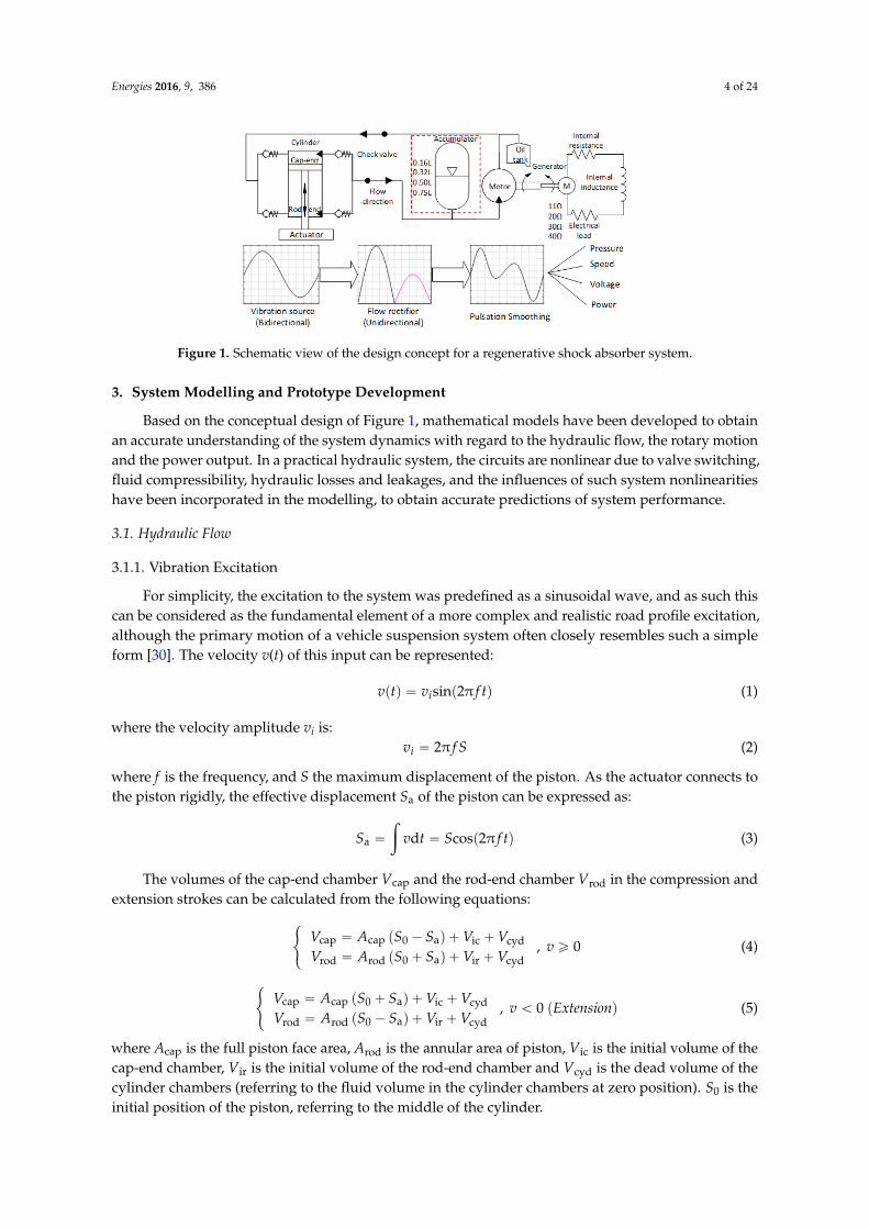
As shown in Figure 1, a schematic design of a regenerative shock absorber which consists of adouble-acting hydraulic cylinder, a hydraulic rectifier in the form of four check valves, a hydraulicaccumulator, a hydraulic motor, a permanent magnetic generator, pipelines and an oil tank is proposed.The key component of the system is the hydraulic cylinder that represents a traditional shock absorber.In the conceptual design, the end of the shock absorber body is fixed to a stationary frame and thepiston rod is connected to a hydraulic actuator which provides oscillatory excitations to representtravel over uneven roads, moving the piston reciprocally. In this paper, the upwards and downwardsmotions of the piston are described as compression and extension, respectively.
The cylinder was designed to have four ports symmetrically distributed at both sides of thecylinder body. As shown in Figure 1, these ports connect to four check valves which act as a hydraulicrectifier. Through rectification, the fluid in both compression and extension motions passes throughthe hydraulic motor in a single direction.
The hydraulic motor is directly coupled to the generator via a shaft and driven by the pressurisedflow. The hydraulic motor converts the linear motion of the piston into rotary motion by transferringoil from the high-pressure side to the low-pressure side, and the subsequent rotation of the motorshaft drives the generator to produce electricity. Road excitation is simulated by a computer controlledactuator, which can be controlled to input several types of excitations, although in this study asinusoidal wave is used as the main excitation input.
Energies 2016, 9, 386 4 of 24
Energies 2016, 9, 386 3 of 23
To compromise between ride health and safety and energy regeneration, automotive
researchers have paid considerable attention to active-regenerative suspension. Zheng and Yu
[24,25] proposed a novel energy-regenerative active suspension. The study focuses on the
performance improvement in ride comfort and the energy regeneration from road vibration. The
results show that the proposed active suspension with control method would be a feasible approach
for a better trade-off between active control and energy regeneration. Furthermore, Xu, Tucker and
Guo [26–28] proposed similar approaches and mechanisms as the MIT design to study an active
shock absorber for energy regeneration. Afterwards, the dynamic features and the feasibility were
investigated by theoretical study and preliminary tests. The damping performance, power
regeneration and ride health and safety were estimated at this initial stage in an attempt to provide
an overview of a regenerative hydraulic suspension system [29].
Although several previous studies utilised a hydraulic rectifier to obtain unidirectional rotation
of motion for power regeneration, parametric studies are necessary to enhance the adaptability and
stability of such a dynamic model. A prototype must be fabricated for model validation and
performance study.
In this paper, a more comprehensive and accurate model of a regenerative hydraulic shock
absorber system is proposed which precisely considers the effects of valve flow, fluid bulk modulus
variation, accumulator smoothing, the influence of generator features, and losses and leakage of the
motor. System parameter identification is used to model the device accurately the proposed model
is then validated under different excitations and load resistances. Thereafter, the influences of
accumulator capacity are evaluated in terms of the pulsation of the entire system, finally the
asymmetric damping characteristics for a conventional hydraulic shock absorber are obtained by
adjusting load resistance and accumulator capacity.
The structure of this paper is as follows: In Section 2, the system schematic of a regenerative
shock absorber system is proposed. Section 3 describes and analyses the mathematical model of a
regenerative shock absorber system which consists of linear oscillations, flow dynamics, rotary
motions, and power regeneration processes. Section 4 presents the prototype system development
and the determination of the system parameters. The evaluation and comparison between prediction
and measurement are then presented in Section 5, and the effects of accumulator capacity are
analysed and studied before conclusions are drawn in Section 6.
2. System Schematic
As shown in Figure 1, a schematic design of a regenerative shock absorber which consists of a
double-acting hydraulic cylinder, a hydraulic rectifier in the form of four check valves, a hydraulic
accumulator, a hydraulic motor, a permanent magnetic generator, pipelines and an oil tank is
proposed. The key component of the system is the hydraulic cylinder that represents a traditional
shock absorber. In the conceptual design, the end of the shock absorber body is fixed to a stationary
frame and the piston rod is connected to a hydraulic actuator which provides oscillatory excitations
to represent travel over uneven roads, moving the piston reciprocally. In this paper, the upwards
and downwards motions of the piston are described as compression and extension, respectively.
Figure 1. Schematic view of the design concept for a regenerative shock absorber system. Figure 1. Schematic view of the design concept for a regenerative shock absorber system.
3. System Modelling and Prototype Development
Based on the conceptual design of Figure 1, mathematical models have been developed to obtainan accurate understanding of the system dynamics with regard to the hydraulic flow, the rotary motionand the power output. In a practical hydraulic system, the circuits are nonlinear due to valve switching,fluid compressibility, hydraulic losses and leakages, and the influences of such system nonlinearitieshave been incorporated in the modelling, to obtain accurate predictions of system performance.
3.1. Hydraulic Flow
3.1.1. Vibration Excitation
For simplicity, the excitation to the system was predefined as a sinusoidal wave, and as such thiscan be considered as the fundamental element of a more complex and realistic road profile excitation,although the primary motion of a vehicle suspension system often closely resembles such a simpleform [30]. The velocity v(t) of this input can be represented:
vptq “ visinp2π f tq (1)
where the velocity amplitude vi is:vi “ 2π f S (2)
where f is the frequency, and S the maximum displacement of the piston. As the actuator connects tothe piston rigidly, the effective displacement Sa of the piston can be expressed as:
Sa “
ż
vdt “ Scosp2π f tq (3)
The volumes of the cap-end chamber Vcap and the rod-end chamber Vrod in the compression andextension strokes can be calculated from the following equations:
#
Vcap “ Acap pS0 ´ Saq `Vic `VcydVrod “ Arod pS0 ` Saq `Vir `Vcyd
, v ě 0 (4)
#
Vcap “ Acap pS0 ` Saq `Vic `VcydVrod “ Arod pS0 ´ Saq `Vir `Vcyd
, v ă 0 pExtensionq (5)
where Acap is the full piston face area, Arod is the annular area of piston, Vic is the initial volume of thecap-end chamber, Vir is the initial volume of the rod-end chamber and Vcyd is the dead volume of thecylinder chambers (referring to the fluid volume in the cylinder chambers at zero position). S0 is theinitial position of the piston, referring to the middle of the cylinder.

Energies 2016, 9, 386 5 of 24
The areas and velocity of the piston are regarded as known parameters. The cap-end pressure Pcap
and the rod-end pressure Prod act on both sides of the piston to generate compression and extensiondamping forces (Fcap and Frod), which are intended to absorb the vibration from road roughness.Hence, the damping force is directly proportional to the pressure output from the shock absorber,meaning that the piston forces can expressed as:
Fcap “ Pcap Acap and Frod “ Prod Arod (6)
where Fcap is the compression piston force and Frod is the extension piston force.To investigate the capability of power regeneration, the power of the piston motion is considered
as the total input power as follows:
Pin “ Pcap Acap |vptq| ` Prod Arod |vptq| (7)
where Pin is the total input power of the piston motion, and |vptq| denotes the instantaneous velocityof the piston.
However, the reciprocating motion of the piston forced by the predefined excitation can generatethe damping force and input power. The fluid will pass through the check valves to rectify the flowand then convert linear motion into unidirectional flow in the pipeline.
3.1.2. Flow across Check Valves
Figure 2 shows the processes of fluid flows in the compression and extension strokes. The effect ofthe check valves is to rectify the cylinder flows Qcout and Qrout from the cap-end and rod-end chambers,hence the flow into the pipelines can be calculated based on Bernoulli’s principle according to:
For flow from the shock absorber :$
’
’
’
’
’
&
’
’
’
’
’
%
Qcout “ Cd Acvsgn`
Pcap ´ Pm ´ Pcv˘
c
2|Pcap´Pm´Pcv|ρ , Pcap ą pPm ` Pcvq ;
Qcout “ 0, Pcap ď pPm ` Pcvq
Qrout “ Cd Acvsgn pProd ´ Pm ´ Pcvq
b
2|Prod´Pm´Pcv|ρ , Prod ą pPm ` Pcvq ;
Qrout “ 0, Prod ď pPm ` Pcvq
(8)
For flow returen to the shock absorber :$
’
’
’
’
’
&
’
’
’
’
’
%
Qcin “ Cd Acvsgn`
Pr ´ Pcap˘
c
2|Pr´Pcap|ρ , Pr ą Pcap;
Qcin “ 0, Pr ď Pcap
Qrin “ Cd Acvsgn pPr ´ Prodq
b
2|Pr´Prod|ρ , Pr ą Prod;
Qrin “ 0, Pr ď Prod
(9)
The flows for returning oil to refill the two cylinder chambers, Qcin and Qrin are shown inEquation (9), where Cd is the discharge coefficient, Acv is the area of the effective check valve port,Pcv is the pre-load pressure of the check valves, Pcap, Prod and Pm represent the pressures at thehigh pressure side of the motor for the cap-end chamber, the rod-end chamber and the motor inletrespectively. ρ is the density of hydraulic fluid. Pr is the total return pressure in the low-pressure side,it is the sum of the return pressures to the cylinder chambers (cap-end chamber: Pcin and rod-endchamber: Prin) during the compression and extension: Pr “ Pcin ` Prin.
Considering the compressibility of hydraulic fluid with the effective bulk modulus in variablechambers, the pressures out of the cylinder chambers during the compression and the extension strokescan be described:
dPcap
dt“βcap
`
Acapv ptq ´Qcout `Qcin˘
VcappCompressionq (10)
Energies 2016, 9, 386 6 of 24
dProddt
“βrod pArod p´v ptqq ´Qrout `Qrinq
VrodpExtensionq (11)
where βcap and βrod are the effective bulk modulus values for the cap-end and rod-end chambers.
Energies 2016, 9, 386 6 of 23
rod rod rout rinrod
rod
βd
d
A v t Q QP
t V
(Extension) (11)
where βcap and βrod are the effective bulk modulus values for the cap-end and rod-end chambers.
With the motion of the piston, the pressurised fluid passes through a set of check valves, the
rectified unidirectional flow is then moved forward to experience the smoothing effect of the
accumulator before passing through the hydraulic motor.
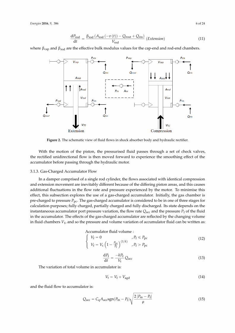
Figure 2. The schematic view of fluid flows in shock absorber body and hydraulic rectifier.
3.1.3. Gas-Charged Accumulator Flow
In a damper comprised of a single rod cylinder, the flows associated with identical compression
and extension movement are inevitably different because of the differing piston areas, and this
causes additional fluctuations in the flow rate and pressure experienced by the motor. To minimise
this effect, this subsection explores the use of a gas-charged accumulator. Initially, the gas chamber is
pre-charged to pressure Ppc. The gas-charged accumulator is considered to be in one of three stages
for calculation purposes; fully charged, partially charged and fully discharged. Its state depends on
the instantaneous accumulator port pressure variation, the flow rate Qacc and the pressure Pf of the
fluid in the accumulator. The effects of the gas-charged accumulator are reflected by the changing
volume in fluid chambers Vf, and so the pressure and volume variation of accumulator fluid can be
written as:
f f pc
1
pc
f c f pc
f
Accumulator fluid volume:
0 ,
1 ,
k
V P P
PV V P P
P
(12)
f f
acc
t
d
d
P k PQ
t V
(13)
The variation of total volume in accumulator is:
t f agdV V V (14)
and the fluid flow to accumulator is:
m f
acc q acc m f
2sgn( )
ρ
P PQ C A P P
(15)
Figure 2. The schematic view of fluid flows in shock absorber body and hydraulic rectifier.
With the motion of the piston, the pressurised fluid passes through a set of check valves,the rectified unidirectional flow is then moved forward to experience the smoothing effect of theaccumulator before passing through the hydraulic motor.
3.1.3. Gas-Charged Accumulator Flow
In a damper comprised of a single rod cylinder, the flows associated with identical compressionand extension movement are inevitably different because of the differing piston areas, and this causesadditional fluctuations in the flow rate and pressure experienced by the motor. To minimise thiseffect, this subsection explores the use of a gas-charged accumulator. Initially, the gas chamber ispre-charged to pressure Ppc. The gas-charged accumulator is considered to be in one of three stages forcalculation purposes; fully charged, partially charged and fully discharged. Its state depends on theinstantaneous accumulator port pressure variation, the flow rate Qacc and the pressure Pf of the fluidin the accumulator. The effects of the gas-charged accumulator are reflected by the changing volumein fluid chambers Vf, and so the pressure and volume variation of accumulator fluid can be written as:
Accumulator fluid volume :$
&
%
Vf “ 0 , Pf ď Ppc
Vf “ Vc
´
1´ PpcPf
¯p1kq, Pf ą Ppc
(12)
dPfdt
“´kPf
VtQacc (13)
The variation of total volume in accumulator is:
Vt “ Vf `Vagd (14)
and the fluid flow to accumulator is:
Qacc “ Cq AaccsgnpPm ´ Pfq
d
2 |Pm ´ Pf|
ρ(15)

Energies 2016, 9, 386 7 of 24
where Vt and Vagd are the total variable volume in the accumulator and the accumulator dead volumerespectively, Aacc is the area of the accumulator inlet port and k is the gas specific heat ratio of thegas-charged accumulator. Certain assumptions have been made to simplify the calculations:
(1) The gas-charged accumulator is assumed to be adiabatic, ignoring the heat exchange thathappens between the gas and oil under conditions of rapid-cycling.
(2) There are no frictions or thermal losses occurring during the charge/discharge cycles in theaccumulator model. When the accumulator is running under variable pressure, thermal lossescaused by variation in the gas temperature will inevitably influence gas behaviour.
(3) The pressures in the fluid chamber instead of those in the gas chamber are used for flow ratecalculation, which is reasonable because of the transient pressure balance inside the accumulator.
However, Equations (14)–(19) indicate that the volume variation of the accumulator fluidchamber can smooth the flow oscillations and hence help to minimise the instability of the fluidflow. The gas-charged accumulator utilises compressed gas to maintain balance between the fluidchamber and the gas chamber, then to stabilise the flow rate through the motor inlet.
3.1.4. Flow through the Hydraulic Motor
With the accumulator mounted upstream of the inlet of the hydraulic motor, the total volume VT
upstream of the motor inlet includes the hydraulic accumulator fluid chamber Vf and the fluid volumeof the pipeline Vl. The pressure loss Ploss in the moving fluid at different flow rates across the pipelineis considered based on the Darcy-Weisbach Equation [31], hence the pressure dPm/dt at the inlet ofthe hydraulic motor is as follows:
dPm
dt“βm pQcout `Qrout ´Qm ´Qaccq
VT(16)
where the volume variation before the motor inlet is:
VT “ Vf `Vl (17)
and the pipeline volume is:Vl “ Ap L (18)
The internal flow leakage in the motor is considered as a development and a more accuratehydraulic motor flow rate can be expressed [32]:
Qm “Dmωm
2π` KlkPm (19)
using the Hagen-Poiseuille coefficient KHP [32]:
KHP “Dmωnom p1´ ηVq σnomρ
Pnom(20)
and the dynamic viscosity of hydraulic oil is:
µ “ σρ (21)
Thereafter, the hydraulic motor leakage coefficient is a mathematical expression of theeffectiveness of the motor leaking and can be written as follows [32]:
Klk “KHP
µ(22)
Energies 2016, 9, 386 8 of 24
with pressure loss in the pipeline of:
Ploss “32σLρpQcout `Qroutq
D2p Acv
(23)
where βm is the effective bulk modulus of the motor chamber, Ap is the cross section of area of the pipe,L is the length of the pipe, Dm is the displacement of the hydraulic motor,ωm is the shaft speed of thehydraulic motor and generator, ηv is the volumetric efficiency of the hydraulic motor, σ is the kineticviscosity of the hydraulic oil, µ is the dynamic viscosity of the hydraulic oil, ωnom is the nominalmotor angular velocity, Pnom is the nominal motor pressure, σnom is the nominal kinetic viscosity ofthe hydraulic oil, ρ is the density of the hydraulic oil, KHP is the Hagen-Poiseuille coefficient, Klk is themotor leakage coefficient and Dp is the diameter of the pipe.
3.2. Rotational Motion
Due to the pressurised flow Qm, the hydraulic motor will rotate with driving torque Tm accordingto the following expression [19]:
Tm “Dm pPm ´ Plossq ηm
2π(24)
where ηm is the mechanical efficiency of the hydraulic motor. To be able to obtain an accuraterepresentation of the rotary motion, a rotational friction torque component Trf was incorporated as aform of mechanical loss, simplified as follows [33]:
Trf “ Cvωm (25)
where Cv is the viscous friction coefficient, andωm is the shaft speed.Using Newton’s second law of motion, the rotary motion can then be written as:
dωm
dt“
Tm ´ Tl ´ TrfJt
(26)
where Jt is the moment of inertia of the shaft and Tl is the electromagnetic torque (described inSection 3.3).
3.3. Electrical Power
In the regenerative power unit of an equivalent DC generator, the electromagnetic torquecoefficient Tl can be expressed using the torque constant coefficient kT and the electric current Ias follows [20]:
Tl “ kT I (27)
and the electromotive force (EMF) E is given by [20]:
E “ kVωm (28)
where kV is the electromotive voltage constant.The dynamic model for the equivalent permanent magnetic DC generator depends on Kirchhoff’s
voltage law [34]. Assuming that the magnet susceptibility at any temperature is constant, as the fluxestablished by the PM poles, the rate of change of current can be expressed as:
dIdt“
E´ pRin ` RLq ILin
(29)
where Lin is the internal inductance of the DC generator, which can be calculated based on measuredvoltages, RL is the load resistance and Rin is the internal resistance.

Energies 2016, 9, 386 9 of 24
The most intuitive means of quantifying the power regeneration is from the instantaneous poweroutput and the power efficiency. In modelling, the regenerated power output Preg can be calculatedfrom the I2R. In testing, the instantaneous voltage U “ RL I at terminals of the load resistance can bemeasured to estimate the potential power output, hence an equivalent expression for Preg can be:
Preg “ I2RL “U2
RL(30)
The regenerated power conversion efficiency ηreg can be defined as the total efficiency of thehydraulic regenerative shock absorber system which can be considered to be the total efficiency andcan be expressed using Equations (27) and (30) as follows:
ηreg “Preg
Pin(31)
3.4. Fabrication of the Prototype
The prototype system was fabricated based around a traditional shock absorber/damper from atypical articulated heavy haulage truck. For such a damper, it has been estimated that the potentialpower that can be recovered is approximately 100–1500 Watts depending on road conditions andtruck loading [35]. Based on the schematic shown in Figure 1, key system components were selectedas summarised in Table 1. Based on the maximum pressure of the cylinder and the motor torque(Equation (24), it was found that an internal gear hydraulic motor meets the requirements of hightorque at low rotational speed.
Table 1. The specifications of main components.
Name Specification
Cylinder Middle point, S0 = 100 mm,Full stroke, 200 mm
Piston area, Dcap = 50 mm,Annulus area, Drod = 30 mm Max. pressure, 200 bar
Motor Displacement,Dm = 8.2 cc (cm3/rev) Max. speed, 245 rad/s Max. power, <6000 W
Generator Internal inductance,Lin = 0.015 H
2.33 Phase magnetic field,Built in rectifier,
Max. speed, 215 rad/s
Max. current, 10 A,Max. power, <2450 W
Accumulator Diaphragm accumulator Port diameter,Dacc = 12.7 mm
Pre-charge pressure,Ppc = 20 bar
Check Valve Diameter: 3/81
(«9.525 mm), BSPP Max. pressure, 350 bar Preload pressure,Pcv = 0.7 bar
Four Post Simulator Maximum velocity, 1.9 m/s Static load, 550 kg Preload, 60 kg
Hose Hose diameter, Dh = 3/81 Length, L = 1 m Max. pressure, 800 bar
Shock Absorber Oil Density, ρ = 872 kg/m3 Viscosity, σ = 22 cSt -
A high inertia PM generator was selected to provide the additional benefits of rotational kineticenergy storage and improved the stability of rotary motion, contributing to the efficiency of powerregeneration. A diaphragm accumulator suitable for a low volume system was connected in front ofthe hydraulic motor to smooth the fluid flow on the high-pressure side by reducing the pulsationsin pressure. According to the damping forces in a conventional shock absorber for a heavy haulagetruck [35], a peak pressure of 35 bar was estimated. The pre-charge pressure in the accumulator wasset at 60% of the working pressure (of 20 bar) to provide pressure pulsation damping.
According to Equations (20)–(23), low viscosity shock absorber oil was used to minimise thelosses in the hydraulic motor and pipework.

Energies 2016, 9, 386 10 of 24
3.5. Test System and Measurement
Via trial and error, numerous refinements were made to the prototype system to permit morereliable and accurate simulation. For example, air bubbles in the fluid within the test system leadto changes in oil viscosity and the bulk modulus, consequently, an air vent valve was employed tominimise the volume of air in the hydraulic fluid and to stabilise the bulk modulus of the oil [36]Furthermore, energy is consumed through compression of the spring in the check valve and to minimisethis effect, the length of the check valve spring was reduced by one-third to reduce pressure losses andimprove dynamic response. In addition, the moving-mass orifices in the check valve were enlargedto allow a greater flow rate and hence to offset valve losses. Finally, based on Equations (19)–(24),the length of the hoses was reduced to minimise pressure losses in the pipelines.
Figure 3 shows how the pressure characteristics of the test system were analysed using twopressure transducers mounted upstream of the diaphragm accumulator port and upstream of thehydraulic motor inlet. A U-shaped micro photo sensor mounted on the shaft coupling was used tomeasure the shaft speed. An electronic load bank was used to vary the load and a voltage transducermeasured the electrical output for analysis of power regeneration and conversion efficiency. All of themeasured outputs were fed into a multi-channel data acquisition system which sampled the data at10 kHz with 14 bit resolution. The measured signals could be observed during experiments in realtime to ensure the correct functioning of the test rig.
Energies 2016, 9, 386 10 of 23
pressure losses and improve dynamic response. In addition, the moving-mass orifices in the check
valve were enlarged to allow a greater flow rate and hence to offset valve losses. Finally, based on
Equations (19)–(24), the length of the hoses was reduced to minimise pressure losses in the pipelines.
Figure 3 shows how the pressure characteristics of the test system were analysed using two
pressure transducers mounted upstream of the diaphragm accumulator port and upstream of the
hydraulic motor inlet. A U-shaped micro photo sensor mounted on the shaft coupling was used to
measure the shaft speed. An electronic load bank was used to vary the load and a voltage transducer
measured the electrical output for analysis of power regeneration and conversion efficiency. All of
the measured outputs were fed into a multi-channel data acquisition system which sampled the data
at 10 kHz with 14 bit resolution. The measured signals could be observed during experiments in real
time to ensure the correct functioning of the test rig.
Real road profiles are often represented as a combination of a number of individual sinusoidal
waves but in this study, for simplicity, a single sinusoidal wave representing the fundamental
frequency of a road surface was used as the system input for both modelling and testing. Such an
approach is not unusual [37], because a single sinusoidal input allows analysis to be performed in a
highly accurate manner and hence a general understanding of the dynamic performances of the
proposed modelling and prototype system can be obtained. During the experimentation, one corner
of a four-post servo-hydraulic ride simulator with a digital control was employed as the source of
vibration to excite the shock absorber system.
Figure 3. Key components of regenerative shock absorber system.
4. Parameter Studies
According to the setup of this prototype system shown in Figure 3, model parameters
associated with geometric dimensions were determined by direct measurement, as shown in Table 2.
The table also shows that discharge and flow coefficients (Cd and Cq) and the specific heat ratio of air
k are parameters where volumes are known.
Figure 3. Key components of regenerative shock absorber system.
Real road profiles are often represented as a combination of a number of individual sinusoidalwaves but in this study, for simplicity, a single sinusoidal wave representing the fundamental frequencyof a road surface was used as the system input for both modelling and testing. Such an approachis not unusual [37], because a single sinusoidal input allows analysis to be performed in a highlyaccurate manner and hence a general understanding of the dynamic performances of the proposedmodelling and prototype system can be obtained. During the experimentation, one corner of afour-post servo-hydraulic ride simulator with a digital control was employed as the source of vibrationto excite the shock absorber system.

Energies 2016, 9, 386 11 of 24
4. Parameter Studies
According to the setup of this prototype system shown in Figure 3, model parameters associatedwith geometric dimensions were determined by direct measurement, as shown in Table 2. The tablealso shows that discharge and flow coefficients (Cd and Cq) and the specific heat ratio of air k areparameters where volumes are known.
Table 2. Hydraulic parameters used in modelling.
Name Symbol Value Unit Name Symbol Value Unit
Accumulator inlet area Aacc 1.27 ˆ 10´4 m2 Flow coefficient Cq 0.7 -
Full piston face area Acap 1.96 ˆ 10´3 m2 Specific heat ratio k 1.4 -
Check valve area Acv 3.93 ˆ 10´5 m2 Cylinder dead volume Vcyd 1 ˆ 10´8 m3
Pipe area Ap 7.85 ˆ 10´5 m2 Accumulator dead volume * Vagd 1%¨Vc m3
Annular area of piston Arod 1.26 ˆ 10´3 m2 Initial volume of cap-end chamber Vic 3.93 ˆ 10´4 m3
Discharge coefficient Cd 0.7 - Initial volume of rod-end chamber Vrc 6.38 ˆ 10´4 m3
* Vc is the accumulator capacity. 0.16 L, 0.32 L, 0.50 L and 0.75 L were used in this study.
The table also shows that there are, however, a number of system parameters whose values areuncertain hence they need to be estimated. As shown in Figure 4, such parameters and variables canbe categorised in two: (1) Parameters related to power generation, including the voltage constantcoefficient kV, the torque constant coefficient kT and the rotational friction torque Trf; and (2) Variablesassociated with hydraulic flow which are the effective bulk modulus of the fluid β (which will bedifferent for the four locations βcap or βrod or βm), the mechanical efficiency ηm and the volumetricefficiency ηv of the hydraulic motor. The objective of this section is to obtain accurate parametersvalues for those parameters in the system which cannot be predetermined. A series of online testswere performed to estimate kV, kT, Rin and Trf in the power regeneration unit. Furthermore, an offlinetest for the generator was designed to confirm the validity of kV and kT. In addition, to determinemore accurately the system behaviour and power output, fluid losses and friction were consideredin modelling and thus ηm and ηv can be calculated for further improvement of the prototype system.From a fluid dynamics modelling standpoint, it is necessary to determine an appropriate bulk modulusmodel of the fluid that is in the hydraulic circuit; this is especially important for high pressurehydraulic systems.
Energies 2016, 9, 386 11 of 23
Table 2. Hydraulic parameters used in modelling.
Name Symbol Value Unit Name Symbol Value Unit
Accumulator inlet area Aacc 1.27 × 10⁻⁴ m2 Flow coefficient Cq 0.7 -
Full piston
face area Acap 1.96 × 10⁻³ m2 Specific heat ratio k 1.4 -
Check valve area Acv 3.93 × 10⁻⁵ m2 Cylinder dead volume Vcyd 1 × 10⁻⁸ m3
Pipe area Ap 7.85 × 10⁻⁵ m2 Accumulator dead volume * Vagd 1%∙Vc m3
Annular area
of piston Arod 1.26 × 10⁻³ m2
Initial volume of
cap-end chamber Vic 3.93 × 10⁻⁴ m3
Discharge coefficient Cd 0.7 - Initial volume of
rod-end chamber Vrc 6.38 × 10⁻⁴ m3
* Vc is the accumulator capacity. 0.16 L, 0.32 L, 0.50 L and 0.75 L were used in this study.
The table also shows that there are, however, a number of system parameters whose values are
uncertain hence they need to be estimated. As shown in Figure 4, such parameters and variables can
be categorised in two: (1) Parameters related to power generation, including the voltage constant
coefficient kV, the torque constant coefficient kT and the rotational friction torque Trf; and (2) Variables
associated with hydraulic flow which are the effective bulk modulus of the fluid β (which will be
different for the four locations βcap or βrod or βm), the mechanical efficiency ηm and the volumetric
efficiency ηv of the hydraulic motor. The objective of this section is to obtain accurate parameters
values for those parameters in the system which cannot be predetermined. A series of online tests
were performed to estimate kV, kT, Rin and Trf in the power regeneration unit. Furthermore, an offline
test for the generator was designed to confirm the validity of kV and kT. In addition, to determine
more accurately the system behaviour and power output, fluid losses and friction were considered
in modelling and thus ηm and ηv can be calculated for further improvement of the prototype system.
From a fluid dynamics modelling standpoint, it is necessary to determine an appropriate bulk
modulus model of the fluid that is in the hydraulic circuit; this is especially important for high
pressure hydraulic systems.
Figure 4. Known and uncertain parameters and variables in power regeneration unit and hydraulic system.
4.1. Power Regeneration System
According to Equations (27)–(31), the performance of the equivalent DC generator to the
rectified alternator used in the study is dependent upon the internal resistance Rin, the voltage constant
coefficient kV and the torque constant coefficient kT. Based on an inverse estimation approach [38],
these parameters were obtained with reference to online speed, current and voltage measurements
under different external loads. Solving Equation (29) obtains the electrical current and then provides
the voltage prediction Upre(kV,i,Rin,j) across the external resistances under a number of incremental voltage
constants kV,i and internal resistances Rin,j. The minimum value of the least square error between the
measured and the predicted voltage according to Equation (32) can then be derived as follows:
Figure 4. Known and uncertain parameters and variables in power regeneration unit andhydraulic system.

Energies 2016, 9, 386 12 of 24
4.1. Power Regeneration System
According to Equations (27)–(31), the performance of the equivalent DC generator to the rectifiedalternator used in the study is dependent upon the internal resistance Rin, the voltage constantcoefficient kV and the torque constant coefficient kT. Based on an inverse estimation approach [38],these parameters were obtained with reference to online speed, current and voltage measurementsunder different external loads. Solving Equation (29) obtains the electrical current and then providesthe voltage prediction Upre(kV,i,Rin,j) across the external resistances under a number of incrementalvoltage constants kV,i and internal resistances Rin,j. The minimum value of the least square errorbetween the measured and the predicted voltage according to Equation (32) can then be derivedas follows:
errorpkV, Rinq “
mÿ
i“1
nÿ
j“1
U ´UprepkV,i, Rin,jq(2 (32)
where U is the measured voltage, Upre represents the voltage prediction for the calculation of theelectrical parameters study, m and n are the numbers of the search processes, and i and j define thesearch starting points.
Figure 5a shows the relationship between the voltage constant and the internal resistance obtainedfrom measurements made directly on the test rig (referred to hereafter as online measurements), andusing four different external resistances. Clearly the optimal internal resistance Rin and the voltageconstant coefficient kV are clearly at the intersection point in Figure 5a, is kV = 0.9256 and Rin = 5.6 Ω.
Energies 2016, 9, 386 12 of 23
2
V in pre V, in,
1 1
error( , ) ( , )m n
i j
i j
k R U U k R
(32)
where U is the measured voltage, Upre represents the voltage prediction for the calculation of the
electrical parameters study, m and n are the numbers of the search processes, and i and j define the
search starting points.
Figure 5a shows the relationship between the voltage constant and the internal resistance obtained
from measurements made directly on the test rig (referred to hereafter as online measurements), and
using four different external resistances. Clearly the optimal internal resistance Rin and the voltage
constant coefficient kV are clearly at the intersection point in Figure 5a, is kV = 0.9256 and Rin = 5.6 Ω.
Figure 5. (a) Online voltage constant coefficient vs internal resistance; (b) online fitted torque
constant coefficient, kT.
Figure 5b shows the relationship between the effective motor torque and instantaneous current,
the gradient of which is the torque constant kT. A parameter that plays an important role in the rotary
motion of the motor and generator unit is the rotational friction torque Trf, and this was given
priority in the estimation of kT. In Equation (25), it can be seen that Trf is proportional to the viscous
friction coefficient and the shaft speed. To obtain an accurate relationship between rotary motion
and regenerative power, a set of online open circuit measurements were taken to find the viscous
coefficient. In these measurements the flow energy or the motor torque Tm is just balanced by the
frictional torque, considering low rate increase process the dynamic torque Jt(dωm/dt) can be
ignored, which leads to the relationship of Equation (33)–(37):
m m loss m
m H m
H m H
H fm
ηη
2π
(1 η )
D P PT T
T T
T T
(33)
where TH is the total output torque of the hydraulic motor and Tfm is the torque due to internal viscous
drag of the hydraulic motor. It will be included into the total friction loss Tf of the system by redefining:
f rf fm v mωT T T C (34)
For the quasi static and open circuit experiments, and hence that Equation (26) can be reset to
dωm/dt ≈ 0 and T1 = 0, the relationship of the torques can then be written as:
m rf 0T T (35)
H fm rf 0T T T (36)
Both Tfm and Trf are due to the friction, which is regarded as the effect of viscous loss:
Figure 5. (a) Online voltage constant coefficient vs internal resistance; (b) online fitted torque constantcoefficient, kT.
Figure 5b shows the relationship between the effective motor torque and instantaneous current,the gradient of which is the torque constant kT. A parameter that plays an important role in therotary motion of the motor and generator unit is the rotational friction torque Trf, and this was givenpriority in the estimation of kT. In Equation (25), it can be seen that Trf is proportional to the viscousfriction coefficient and the shaft speed. To obtain an accurate relationship between rotary motion andregenerative power, a set of online open circuit measurements were taken to find the viscous coefficient.In these measurements the flow energy or the motor torque Tm is just balanced by the frictional torque,considering low rate increase process the dynamic torque Jt(dωm/dt) can be ignored, which leads tothe relationship of Equations (33)–(37):
Tm “Dm pPm´Plossqηm
2π “ THηm“ TH ´ p1´ ηmqTH
“ TH ´ Tfm
(33)
Energies 2016, 9, 386 13 of 24
where TH is the total output torque of the hydraulic motor and Tfm is the torque due to internal viscousdrag of the hydraulic motor. It will be included into the total friction loss Tf of the system by redefining:
Tf “ Trf ` Tfm “ Cvωm (34)
For the quasi static and open circuit experiments, and hence that Equation (26) can be reset todωm/dt « 0 and T1 = 0, the relationship of the torques can then be written as:
Tm ´ Trf “ 0 (35)
TH ´ Tfm ´ Trf “ 0 (36)
Both Tfm and Trf are due to the friction, which is regarded as the effect of viscous loss:
TH “ Tfm ` Trf “ frictional torque “ Cvωm (37)
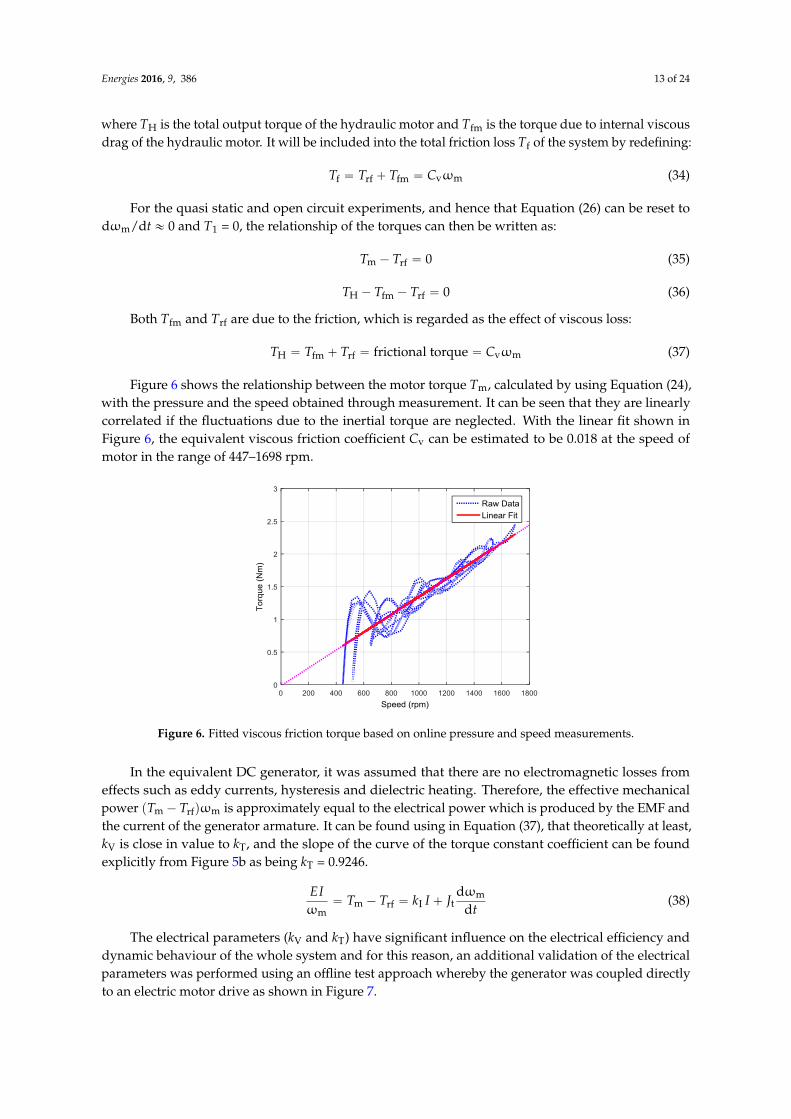
Figure 6 shows the relationship between the motor torque Tm, calculated by using Equation (24),with the pressure and the speed obtained through measurement. It can be seen that they are linearlycorrelated if the fluctuations due to the inertial torque are neglected. With the linear fit shown inFigure 6, the equivalent viscous friction coefficient Cv can be estimated to be 0.018 at the speed ofmotor in the range of 447–1698 rpm.
Energies 2016, 9, 386 13 of 23
H fm rf v mfrictional torque ωT T T C (37)
Figure 6 shows the relationship between the motor torque Tm, calculated by using Equation (24),
with the pressure and the speed obtained through measurement. It can be seen that they are linearly
correlated if the fluctuations due to the inertial torque are neglected. With the linear fit shown in
Figure 6, the equivalent viscous friction coefficient Cv can be estimated to be 0.018 at the speed of
motor in the range of 447–1698 rpm.
Figure 6. Fitted viscous friction torque based on online pressure and speed measurements.
In the equivalent DC generator, it was assumed that there are no electromagnetic losses from
effects such as eddy currents, hysteresis and dielectric heating. Therefore, the effective mechanical
power m rf m( )ωT T is approximately equal to the electrical power which is produced by the EMF
and the current of the generator armature. It can be found using in Equation (37), that theoretically at
least, kV is close in value to kT, and the slope of the curve of the torque constant coefficient can be
found explicitly from Figure 5b as being kT = 0.9246.
m
m rf I t
m
dω
ω d
E IT T k I J
t (38)
The electrical parameters (kV and kT) have significant influence on the electrical efficiency and
dynamic behaviour of the whole system and for this reason, an additional validation of the electrical
parameters was performed using an offline test approach whereby the generator was coupled
directly to an electric motor drive as shown in Figure 7.
Figure 7. View of experimental generator test set up.
In the directly coupled offline test, an electrical load was set to values of 11, 20, 30 and 40 Ω, and
the mean voltage and current were measured at 150, 300, 450, 600, 750 and 900 rpm for each value of
resistance. The average torque was calculated by a programmable logic controller (PLC), and the
results are shown in Figure 8a,b.
Figure 6. Fitted viscous friction torque based on online pressure and speed measurements.
In the equivalent DC generator, it was assumed that there are no electromagnetic losses fromeffects such as eddy currents, hysteresis and dielectric heating. Therefore, the effective mechanicalpower pTm ´ Trfqωm is approximately equal to the electrical power which is produced by the EMF andthe current of the generator armature. It can be found using in Equation (37), that theoretically at least,kV is close in value to kT, and the slope of the curve of the torque constant coefficient can be foundexplicitly from Figure 5b as being kT = 0.9246.
EIωm
“ Tm ´ Trf “ kI I ` Jtdωm
dt(38)
The electrical parameters (kV and kT) have significant influence on the electrical efficiency anddynamic behaviour of the whole system and for this reason, an additional validation of the electricalparameters was performed using an offline test approach whereby the generator was coupled directlyto an electric motor drive as shown in Figure 7.

Energies 2016, 9, 386 14 of 24
Energies 2016, 9, 386 13 of 23
H fm rf v mfrictional torque ωT T T C (37)
Figure 6 shows the relationship between the motor torque Tm, calculated by using Equation (24),
with the pressure and the speed obtained through measurement. It can be seen that they are linearly
correlated if the fluctuations due to the inertial torque are neglected. With the linear fit shown in
Figure 6, the equivalent viscous friction coefficient Cv can be estimated to be 0.018 at the speed of
motor in the range of 447–1698 rpm.
Figure 6. Fitted viscous friction torque based on online pressure and speed measurements.
In the equivalent DC generator, it was assumed that there are no electromagnetic losses from
effects such as eddy currents, hysteresis and dielectric heating. Therefore, the effective mechanical
power m rf m( )ωT T is approximately equal to the electrical power which is produced by the EMF
and the current of the generator armature. It can be found using in Equation (37), that theoretically at
least, kV is close in value to kT, and the slope of the curve of the torque constant coefficient can be
found explicitly from Figure 5b as being kT = 0.9246.
m
m rf I t
m
dω
ω d
E IT T k I J
t (38)
The electrical parameters (kV and kT) have significant influence on the electrical efficiency and
dynamic behaviour of the whole system and for this reason, an additional validation of the electrical
parameters was performed using an offline test approach whereby the generator was coupled
directly to an electric motor drive as shown in Figure 7.
Figure 7. View of experimental generator test set up.
In the directly coupled offline test, an electrical load was set to values of 11, 20, 30 and 40 Ω, and
the mean voltage and current were measured at 150, 300, 450, 600, 750 and 900 rpm for each value of
resistance. The average torque was calculated by a programmable logic controller (PLC), and the
results are shown in Figure 8a,b.
Figure 7. View of experimental generator test set up.
In the directly coupled offline test, an electrical load was set to values of 11, 20, 30 and 40 Ω, andthe mean voltage and current were measured at 150, 300, 450, 600, 750 and 900 rpm for each valueof resistance. The average torque was calculated by a programmable logic controller (PLC), and theresults are shown in Figure 8a,b.Energies 2016, 9, 386 14 of 23
Figure 8. (a) Offline fitted voltage constant; (b) offline fitted torque constant.
The offline tests provided the following values for voltage constant coefficient and torque
constant coefficient, kV = 0.9303 and kT = 0.9274, these compare to online estimations of kV = 0.9256 and
kT = 0.9246, showing that there is close agreement between the estimation approaches and also that
kV and kT are very similar in value.
4.2. Hydraulic System
In this study, the mechanical and volumetric efficiencies in the hydraulic motor and the
effective bulk modulus of the hydraulic fluid, were determined by modelling of the hydraulic
system. In modelling, the assumptions made during this process were as follows:
Firstly, the hydraulic cylinder was assumed to be frictionless and without leakage.
Secondly, in Equation (20), the mean values of the time-varying pressure and speed of the
motor were taken as the nominal pressure drop (for the calculation of the hydraulic motor
leakage coefficient) and the nominal shaft speed, respectively.
Thirdly, the values of kT and kV were used as determined in Subsection 4.1, meaning that
there are no additional electrical losses in the generator model to be accounted for, hence it
can be assumed that the hydraulic motor power output Pm is equal to the power captured in
the generator Pcap.
Mechanical and volumetric losses are the main influences on the hydraulic motor’s efficiency.
Based on the above-mentioned assumptions, the mechanical efficiency ηm can be expressed as:
m m loss rf
m
m m loss
( ) 2πη
( )
D P P T
D P P
(39)
The ratio of the Pcap to the initial input power Pin is defined as generator captured efficiency ηcap
and expressed by Equation (41). The volumetric efficiency ηv of the motor was calculated using the
captured power efficiency ηcap in the generator and the mechanical efficiency ηm in the hydraulic
motor. Therefore, the ηv can be defined as:
2
cap in L( )P I R R (40)
cap
cap
in
ηP
P (41)
cap
v
m
ηη
η (42)
The effective bulk modulus of the fluid is representative of its compressibility and is the gauge
of stiffness within the hydraulic system; this will vary with temperature and the amount of
Figure 8. (a) Offline fitted voltage constant; (b) offline fitted torque constant.
The offline tests provided the following values for voltage constant coefficient and torque constantcoefficient, kV = 0.9303 and kT = 0.9274, these compare to online estimations of kV = 0.9256 andkT = 0.9246, showing that there is close agreement between the estimation approaches and also that kV
and kT are very similar in value.
4.2. Hydraulic System
In this study, the mechanical and volumetric efficiencies in the hydraulic motor and the effectivebulk modulus of the hydraulic fluid, were determined by modelling of the hydraulic system.In modelling, the assumptions made during this process were as follows:
‚ Firstly, the hydraulic cylinder was assumed to be frictionless and without leakage.‚ Secondly, in Equation (20), the mean values of the time-varying pressure and speed of the motor
were taken as the nominal pressure drop (for the calculation of the hydraulic motor leakagecoefficient) and the nominal shaft speed, respectively.
‚ Thirdly, the values of kT and kV were used as determined in Section 4.1, meaning that there are noadditional electrical losses in the generator model to be accounted for, hence it can be assumedthat the hydraulic motor power output Pm is equal to the power captured in the generator Pcap.

Energies 2016, 9, 386 15 of 24
Mechanical and volumetric losses are the main influences on the hydraulic motor’s efficiency.Based on the above-mentioned assumptions, the mechanical efficiency ηm can be expressed as:
ηm “DmpPm ´ Plossq ´ 2πTrf
DmpPm ´ Plossq(39)
The ratio of the Pcap to the initial input power Pin is defined as generator captured efficiency ηcap
and expressed by Equation (41). The volumetric efficiency ηv of the motor was calculated using thecaptured power efficiency ηcap in the generator and the mechanical efficiency ηm in the hydraulicmotor. Therefore, the ηv can be defined as:
Pcap “ I2pRin ` RLq (40)
ηcap “Pcap
Pin(41)
ηv “ηcap
ηm(42)
The effective bulk modulus of the fluid is representative of its compressibility and is the gauge ofstiffness within the hydraulic system; this will vary with temperature and the amount of entrained air.In any hydraulic system, hydraulic fluid is always accompanied by a small amount of non-dissolvedand entrained gas, which can be quantified by the gas ratio α. Any entrained air will cause airbubbles that will significantly reduce the bulk modulus value and hence adversely affect the powerregeneration capability. The effective bulk modulus was estimated to vary nonlinearly with pressure,as shown in Figure 9, and as described below.
Energies 2016, 9, 386 15 of 23
entrained air. In any hydraulic system, hydraulic fluid is always accompanied by a small amount of
non-dissolved and entrained gas, which can be quantified by the gas ratio α. Any entrained air will
cause air bubbles that will significantly reduce the bulk modulus value and hence adversely affect the
power regeneration capability. The effective bulk modulus was estimated to vary nonlinearly with
pressure, as shown in Figure 9, and as described below.
Figure 9. (a) Bulk modulus variation with motor pressure; (b) predicted motor pressures for
different bulk modulus values.
The effects of entrained air and mechanical compliance can be determined from direct
measurements then using fundamental effects, the entrained air as proposed by Backe and
Murrenhoff [39] in the following formulae for the isentropic bulk modulus of liquid-air mixtures
(air ratio α), can be calculated as follows:
a
a
e ref 1/
aref1
a
1 α
β β
1 α β
( )
k
k
k
P
P P
P
n P P
(43)
where Pa is the atmospheric pressure, n is the gas specific heat ratio, and P is the relevant pressure
(Pcap, Prod or Pm).
Generally, there are a several empirical determinations for effective bulk modulus. Boes’s
model [40] is the one of the more commonly used for a hydraulic cylinder based system, and has
been used in this study because of its simplicity and specific application to low pressure systems
(under 100 bar). In accordance with the guidelines for hydraulic system modelling from the Institute
for Fluid Power Drives and Controls, Rheinisch-Westfälische Technische Hochschule (RWTH)
Aachen, Germany [39,40], the application specific parameter values of 0.5, 99 and 1 in Equation (44)
were selected because the system in a low pressure system [40].
The Boes’ Model used is hence:
e ref
ref
β 0.5 β log 99 1P
P
(44)
In the Boes’ model, the reference bulk modulus βref and the reference pressure Pref are constants
and the values used are 1.2 × 10⁹ Pa and 1 × 10⁷ Pa respectively, again selected using the guideline in
[40]. To calculate the effective bulk modulus, the gas ratio α was set to values of 0, 0.01, and 0.02
which are typical of a hydraulic cylinder [39]. For the same operating conditions, the smaller the
predefined air ratio, the larger the motor pressure due to the reduced compressibility of the fluid. In
real applications, it can be difficult to define a proper air ratio due to the variable solubility of the
gas, which is dependent on both temperature and working pressure, and in Figure 9, the Boes’ bulk
Figure 9. (a) Bulk modulus variation with motor pressure; (b) predicted motor pressures for differentbulk modulus values.
The effects of entrained air and mechanical compliance can be determined from directmeasurements then using fundamental effects, the entrained air as proposed by Backe andMurrenhoff [39] in the following formulae for the isentropic bulk modulus of liquid-air mixtures(air ratio α), can be calculated as follows:
βe “ βref
1`α´
PaPa`P
¯
1`α Pa1k
n¨pPa`Pqk`1
kβref
(43)

Energies 2016, 9, 386 16 of 24
where Pa is the atmospheric pressure, n is the gas specific heat ratio, and P is the relevant pressure(Pcap, Prod or Pm).
Generally, there are a several empirical determinations for effective bulk modulus. Boes’smodel [40] is the one of the more commonly used for a hydraulic cylinder based system, and has beenused in this study because of its simplicity and specific application to low pressure systems (under100 bar). In accordance with the guidelines for hydraulic system modelling from the Institute forFluid Power Drives and Controls, Rheinisch-Westfälische Technische Hochschule (RWTH) Aachen,Germany [39,40], the application specific parameter values of 0.5, 99 and 1 in Equation (44) wereselected because the system in a low pressure system [40].
The Boes’ Model used is hence:
βe “ 0.5 ¨βref ¨ logˆ
99P
Pref` 1
˙
(44)
In the Boes’ model, the reference bulk modulus βref and the reference pressure Pref are constantsand the values used are 1.2 ˆ 109 Pa and 1 ˆ 107 Pa respectively, again selected using the guidelinein [40]. To calculate the effective bulk modulus, the gas ratio α was set to values of 0, 0.01, and 0.02which are typical of a hydraulic cylinder [39]. For the same operating conditions, the smaller thepredefined air ratio, the larger the motor pressure due to the reduced compressibility of the fluid. Inreal applications, it can be difficult to define a proper air ratio due to the variable solubility of thegas, which is dependent on both temperature and working pressure, and in Figure 9, the Boes’ bulkmodulus shows a large variation from 9860 bar to 12,450 bar. The expressions for the determinedeffective bulk modulus are values shown in Equations (45)–(47):
βcap “ 0.5 ¨βref ¨ logˆ
99 ¨Pcap
Pref` 1
˙
pCap´ endchamberq (45)
βrod “ 0.5 ¨βref ¨ logˆ
99 ¨ProdPref
` 1˙
pRod´ endchamberq (46)
βm “ 0.5 ¨βref ¨ logˆ
99 ¨Pm
Pref` 1
˙
pHydraulicdmotorchamberq (47)
At this point, all of the parameter originally identified in Figure 4 as “To Be Determined” can nowbe quantified, and expressions have been determined for all of the variables as follows in Figure 10:
Energies 2016, 9, 386 16 of 23
modulus shows a large variation from 9860 bar to 12,450 bar. The expressions for the determined
effective bulk modulus are values shown in Equations (45)–(47):
cap
cap ref
ref
β =0.5 β log 99 1P
P
(Cap-end chamber) (45)
rod
rod ref
ref
β =0.5 β log 99 1P
P
(Rod-end chamber) (46)
m
m ref
ref
β =0.5 β log 99 1P
P
(Hydraulic motor chamber) (47)
At this point, all of the parameter originally identified in Figure 4 as “To Be Determined” can
now be quantified, and expressions have been determined for all of the variables as follows in Figure 10:
Figure 10. Determined parameters and variables in power regeneration unit and hydraulic system.
5. Results and Discussion
To validate the model predicted behaviour, the test facility described in Section 3.5 was used
under different excitations and load resistances. In addition, the effects of the accumulator capacity
were also considered. In both modelling and testing, the predefined excitations are consistent with
the open circuit measurements for the estimation of the viscous friction coefficient in Section 4.1.
5.1. Validation Using Excitations
Clearly, the main source of vibration of a vehicle is the excitation input from the road surface.
For this reason the first model validation applied different excitations of 0.5 Hz, 25 mm and 1 Hz,
20 mm, both using an accumulator volume of 0.16 L and a load resistance of 11 Ω. The performance
study focused on the variations between the motor pressure drop and the rotational motion. Using
the refined parameters of the proposed system obtained from the parameter identification study of
Section 4, close agreement between the measured and predicted results was obtained. The hydraulic
motor inlet pressure and the shaft speed differences between prediction and measurement are
shown in Figures 11 and 12. It can be seen that higher excitation causes greater pressure, hence
results in higher motor speed.
Figure 10. Determined parameters and variables in power regeneration unit and hydraulic system.

Energies 2016, 9, 386 17 of 24
5. Results and Discussion
To validate the model predicted behaviour, the test facility described in Section 3.5 was usedunder different excitations and load resistances. In addition, the effects of the accumulator capacitywere also considered. In both modelling and testing, the predefined excitations are consistent with theopen circuit measurements for the estimation of the viscous friction coefficient in Section 4.1.
5.1. Validation Using Excitations
Clearly, the main source of vibration of a vehicle is the excitation input from the road surface.For this reason the first model validation applied different excitations of 0.5 Hz, 25 mm and 1 Hz,20 mm, both using an accumulator volume of 0.16 L and a load resistance of 11 Ω. The performancestudy focused on the variations between the motor pressure drop and the rotational motion. Usingthe refined parameters of the proposed system obtained from the parameter identification study ofSection 4, close agreement between the measured and predicted results was obtained. The hydraulicmotor inlet pressure and the shaft speed differences between prediction and measurement are shownin Figures 11 and 12. It can be seen that higher excitation causes greater pressure, hence results inhigher motor speed.Energies 2016, 9, 386 17 of 23
Figure 11. Predicted and measured pressure at (a) 0.5 Hz frequency and 25 mm amplitude; and (b)
1.0 Hz frequency and 20 mm amplitude (R is equal to the external load RL and V is the same as
accumulator capacity Vc).
Figure 12. Predicted and measured motor speed at (a) 0.5 Hz frequency and 25 mm amplitude; and
(b) 1.0 Hz frequency and 20 mm amplitude.
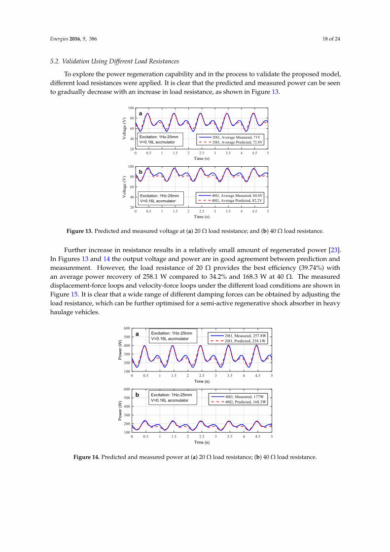
5.2. Validation Using Different Load Resistances
To explore the power regeneration capability and in the process to validate the proposed
model, different load resistances were applied. It is clear that the predicted and measured power can
be seen to gradually decrease with an increase in load resistance, as shown in Figure 13.
Figure 13. Predicted and measured voltage at (a) 20 Ω load resistance; and (b) 40 Ω load resistance.
Figure 11. Predicted and measured pressure at (a) 0.5 Hz frequency and 25 mm amplitude; and(b) 1.0 Hz frequency and 20 mm amplitude (R is equal to the external load RL and V is the same asaccumulator capacity Vc).
Energies 2016, 9, 386 17 of 23
Figure 11. Predicted and measured pressure at (a) 0.5 Hz frequency and 25 mm amplitude; and (b)
1.0 Hz frequency and 20 mm amplitude (R is equal to the external load RL and V is the same as
accumulator capacity Vc).
Figure 12. Predicted and measured motor speed at (a) 0.5 Hz frequency and 25 mm amplitude; and
(b) 1.0 Hz frequency and 20 mm amplitude.
5.2. Validation Using Different Load Resistances
To explore the power regeneration capability and in the process to validate the proposed
model, different load resistances were applied. It is clear that the predicted and measured power can
be seen to gradually decrease with an increase in load resistance, as shown in Figure 13.
Figure 13. Predicted and measured voltage at (a) 20 Ω load resistance; and (b) 40 Ω load resistance.
Figure 12. Predicted and measured motor speed at (a) 0.5 Hz frequency and 25 mm amplitude; and(b) 1.0 Hz frequency and 20 mm amplitude.
Energies 2016, 9, 386 18 of 24
5.2. Validation Using Different Load Resistances
To explore the power regeneration capability and in the process to validate the proposed model,different load resistances were applied. It is clear that the predicted and measured power can be seento gradually decrease with an increase in load resistance, as shown in Figure 13.
Energies 2016, 9, 386 17 of 23
Figure 11. Predicted and measured pressure at (a) 0.5 Hz frequency and 25 mm amplitude; and (b)
1.0 Hz frequency and 20 mm amplitude (R is equal to the external load RL and V is the same as
accumulator capacity Vc).
Figure 12. Predicted and measured motor speed at (a) 0.5 Hz frequency and 25 mm amplitude; and
(b) 1.0 Hz frequency and 20 mm amplitude.
5.2. Validation Using Different Load Resistances
To explore the power regeneration capability and in the process to validate the proposed
model, different load resistances were applied. It is clear that the predicted and measured power can
be seen to gradually decrease with an increase in load resistance, as shown in Figure 13.
Figure 13. Predicted and measured voltage at (a) 20 Ω load resistance; and (b) 40 Ω load resistance. Figure 13. Predicted and measured voltage at (a) 20 Ω load resistance; and (b) 40 Ω load resistance.
Further increase in resistance results in a relatively small amount of regenerated power [23].In Figures 13 and 14 the output voltage and power are in good agreement between prediction andmeasurement. However, the load resistance of 20 Ω provides the best efficiency (39.74%) withan average power recovery of 258.1 W compared to 34.2% and 168.3 W at 40 Ω. The measureddisplacement-force loops and velocity-force loops under the different load conditions are shown inFigure 15. It is clear that a wide range of different damping forces can be obtained by adjusting theload resistance, which can be further optimised for a semi-active regenerative shock absorber in heavyhaulage vehicles.
Energies 2016, 9, 386 18 of 23
Further increase in resistance results in a relatively small amount of regenerated power [23]. In
Figures 13 and 14, the output voltage and power are in good agreement between prediction and
measurement. However, the load resistance of 20 Ω provides the best efficiency (39.74%) with
an average power recovery of 258.1 W compared to 34.2% and 168.3 W at 40 Ω. The measured
displacement-force loops and velocity-force loops under the different load conditions are shown in
Figure 15. It is clear that a wide range of different damping forces can be obtained by adjusting the
load resistance, which can be further optimised for a semi-active regenerative shock absorber in
heavy haulage vehicles.
Figure 14. Predicted and measured power at (a) 20 Ω load resistance; (b) 40 Ω load resistance.
Figure 15. (a) Measured displacement-force loops; (b) measured velocity-force loops, at 11 Ω, 20 Ω,
30 Ω and 40 Ω load resistances.
5.3. The effect of Accumulator Capacity
Testing under 1 Hz frequency and 25 mm amplitude excitation, with an optimal load resistance
of 20 Ω, was then evaluated at different accumulator capacities and the predicted and measured
results are displayed in Figures 16 and 17. The motor pressure and regenerated power shows close
correlation between measurement and prediction. However, there is a slightly greater inconsistency
between the predicted and the measured shaft speeds. With increasing accumulator capacities, the
peak values of the shaft speed corresponding to the cap-end pressure decreased, representing an
inverse variation with those in the modelling, this effect increases with accumulator capacity.
Figure 14. Predicted and measured power at (a) 20 Ω load resistance; (b) 40 Ω load resistance.

Energies 2016, 9, 386 19 of 24
Energies 2016, 9, 386 18 of 23
Further increase in resistance results in a relatively small amount of regenerated power [23]. In
Figures 13 and 14, the output voltage and power are in good agreement between prediction and
measurement. However, the load resistance of 20 Ω provides the best efficiency (39.74%) with
an average power recovery of 258.1 W compared to 34.2% and 168.3 W at 40 Ω. The measured
displacement-force loops and velocity-force loops under the different load conditions are shown in
Figure 15. It is clear that a wide range of different damping forces can be obtained by adjusting the
load resistance, which can be further optimised for a semi-active regenerative shock absorber in
heavy haulage vehicles.
Figure 14. Predicted and measured power at (a) 20 Ω load resistance; (b) 40 Ω load resistance.
Figure 15. (a) Measured displacement-force loops; (b) measured velocity-force loops, at 11 Ω, 20 Ω,
30 Ω and 40 Ω load resistances.
5.3. The effect of Accumulator Capacity
Testing under 1 Hz frequency and 25 mm amplitude excitation, with an optimal load resistance
of 20 Ω, was then evaluated at different accumulator capacities and the predicted and measured
results are displayed in Figures 16 and 17. The motor pressure and regenerated power shows close
correlation between measurement and prediction. However, there is a slightly greater inconsistency
between the predicted and the measured shaft speeds. With increasing accumulator capacities, the
peak values of the shaft speed corresponding to the cap-end pressure decreased, representing an
inverse variation with those in the modelling, this effect increases with accumulator capacity.
Figure 15. (a) Measured displacement-force loops; (b) measured velocity-force loops, at 11 Ω, 20 Ω,30 Ω and 40 Ω load resistances.
5.3. The effect of Accumulator Capacity
Testing under 1 Hz frequency and 25 mm amplitude excitation, with an optimal load resistance of20 Ω, was then evaluated at different accumulator capacities and the predicted and measured resultsare displayed in Figures 16 and 17. The motor pressure and regenerated power shows close correlationbetween measurement and prediction. However, there is a slightly greater inconsistency between thepredicted and the measured shaft speeds. With increasing accumulator capacities, the peak values ofthe shaft speed corresponding to the cap-end pressure decreased, representing an inverse variationwith those in the modelling, this effect increases with accumulator capacity.Energies 2016, 9, 386 19 of 23
Figure 16. (a) Predicted motor pressure; (b) predicted shaft speed; (c) predicted regenerative power;
(d) predicted power regeneration efficiency, at 0.16 L, 0.32 L, 0.50 L and 0.75 L accumulator capacities.
Figure 17. (a) Measured motor pressure; (b) measured shaft speed; (c) measured regenerative power;
(d) measured power regeneration efficiency, at 0.16 L, 0.32 L, 0.50 L and 0.75 L accumulator capacity.
The motor outlet pressure in the test system was not uniform although it had been set as a
constant in the model, and the effective pressure drop in the motor chamber was smaller than that
used in modelling. In Figures 16b and 17b, it can be seen that the average and peak values of the
Figure 16. (a) Predicted motor pressure; (b) predicted shaft speed; (c) predicted regenerative power;(d) predicted power regeneration efficiency, at 0.16 L, 0.32 L, 0.50 L and 0.75 L accumulator capacities.

Energies 2016, 9, 386 20 of 24
Energies 2016, 9, 386 19 of 23
Figure 16. (a) Predicted motor pressure; (b) predicted shaft speed; (c) predicted regenerative power;
(d) predicted power regeneration efficiency, at 0.16 L, 0.32 L, 0.50 L and 0.75 L accumulator capacities.
Figure 17. (a) Measured motor pressure; (b) measured shaft speed; (c) measured regenerative power;
(d) measured power regeneration efficiency, at 0.16 L, 0.32 L, 0.50 L and 0.75 L accumulator capacity.
The motor outlet pressure in the test system was not uniform although it had been set as a
constant in the model, and the effective pressure drop in the motor chamber was smaller than that
used in modelling. In Figures 16b and 17b, it can be seen that the average and peak values of the
Figure 17. (a) Measured motor pressure; (b) measured shaft speed; (c) measured regenerative power;(d) measured power regeneration efficiency, at 0.16 L, 0.32 L, 0.50 L and 0.75 L accumulator capacity.
The motor outlet pressure in the test system was not uniform although it had been set as a constantin the model, and the effective pressure drop in the motor chamber was smaller than that used inmodelling. In Figures 16b and 17b, it can be seen that the average and peak values of the shaft speedare smaller than those used in modelling. In addition, the deflection of the test rig frame leads toan inevitable small misalignment between the motor and generator shaft, which in turn reduces theeffective motor torque and shaft speed.
The inherent characteristics of a diaphragm accumulator are such that it can prevent fluid shocksfrom highly oscillating flows and also balance pulsations of the fluid with only a small amount ofthe pressure consumption. The accumulator is therefore able to operate as a pressure compensationelement or energy storage device in a low pressure process to provide the continuity and stability ofthe pressurised flow. Figures 16a and 17a show that the mean pressure after the accumulator port(which is upstream of the motor inlet) is around 41 bar, and the power outputs and the regenerationefficiency are approximately 260 W and 40%, respectively. It can also be seen from Figures 16 and 17that increase in accumulator capacity from 0.16 L to 0.75 L can improve the stability of the entire systemwithout significantly influencing the average motor inlet pressure, shaft speed or power.
Additionally, based on the experimental work, the volumetric efficiency of the hydraulic motorcan be obtained by using the ratio of actual fluid flow out of the hydraulic motor to total theoreticalfluid flow out of the shock absorber chambers. Therefore, the calculation process is given and shownin Figure 18. It assumes that the total fluid flow QT is equal to the theoretical flows from the shockabsorber body (Qcap,m and Qrod,m) which is actuated by the excitation input v(t). The hydraulic motorflow can be calculated by using the displacement of the motor and measured motor speeds, then theaverage volumetric efficiency can also be estimated for measured results. The measured volumetricefficiency therefore can be provided to validate against the predictions. However, Figure 19 shows thatthe predicted and measured volumetric efficiency are in good agreement. It also indicates that the effectof accumulator capacity can efficiently stabilise the system behaviours with acceptable recoverablepower, and also the volumetric efficiency and the regeneration efficiency are changed very slightly.

Energies 2016, 9, 386 21 of 24
Energies 2016, 9, 386 20 of 23
shaft speed are smaller than those used in modelling. In addition, the deflection of the test rig frame
leads to an inevitable small misalignment between the motor and generator shaft, which in turn
reduces the effective motor torque and shaft speed.
The inherent characteristics of a diaphragm accumulator are such that it can prevent fluid
shocks from highly oscillating flows and also balance pulsations of the fluid with only a small
amount of the pressure consumption. The accumulator is therefore able to operate as a pressure
compensation element or energy storage device in a low pressure process to provide the continuity
and stability of the pressurised flow. Figures 16a and 17a show that the mean pressure after the
accumulator port (which is upstream of the motor inlet) is around 41 bar, and the power outputs and
the regeneration efficiency are approximately 260 W and 40%, respectively. It can also be seen from
Figures 16 and 17 that increase in accumulator capacity from 0.16 L to 0.75 L can improve the
stability of the entire system without significantly influencing the average motor inlet pressure, shaft
speed or power.
Additionally, based on the experimental work, the volumetric efficiency of the hydraulic motor
can be obtained by using the ratio of actual fluid flow out of the hydraulic motor to total theoretical
fluid flow out of the shock absorber chambers. Therefore, the calculation process is given and shown
in Figure 18. It assumes that the total fluid flow QT is equal to the theoretical flows from the shock
absorber body (Qcap,m and Qrod,m) which is actuated by the excitation input v(t). The hydraulic motor
flow can be calculated by using the displacement of the motor and measured motor speeds, then the
average volumetric efficiency can also be estimated for measured results. The measured volumetric
efficiency therefore can be provided to validate against the predictions. However, Figure 19 shows
that the predicted and measured volumetric efficiency are in good agreement. It also indicates that
the effect of accumulator capacity can efficiently stabilise the system behaviours with acceptable
recoverable power, and also the volumetric efficiency and the regeneration efficiency are changed
very slightly.
Figure 18. The calculation process of the measured volumetric efficiency.
Figure 19. Hydraulic motor volumetric efficiency between predictions and measurements at 0.16 L,
0.32 L, 0.50 L and 0.75 L accumulator capacities.
In the measured displacement-force loops and velocity-force loops, which are shown in Figure 20,
it can be seen that the forces on the piston (equivalent to damping forces) are further stabilised and
regulated during the compression stroke by increasing the accumulator capacity and that the peaks
decrease from 11.46 kN to 9.33 kN (close to a 20% reduction). The peak values of the damping forces
at 0.5 L and 0.75 L accumulator volumes are similar in the compression and extension strokes
because these are appropriate accumulator capacities for the magnitude of excitation.
Figure 18. The calculation process of the measured volumetric efficiency.
Energies 2016, 9, 386 20 of 23
shaft speed are smaller than those used in modelling. In addition, the deflection of the test rig frame
leads to an inevitable small misalignment between the motor and generator shaft, which in turn
reduces the effective motor torque and shaft speed.
The inherent characteristics of a diaphragm accumulator are such that it can prevent fluid
shocks from highly oscillating flows and also balance pulsations of the fluid with only a small
amount of the pressure consumption. The accumulator is therefore able to operate as a pressure
compensation element or energy storage device in a low pressure process to provide the continuity
and stability of the pressurised flow. Figures 16a and 17a show that the mean pressure after the
accumulator port (which is upstream of the motor inlet) is around 41 bar, and the power outputs and
the regeneration efficiency are approximately 260 W and 40%, respectively. It can also be seen from
Figures 16 and 17 that increase in accumulator capacity from 0.16 L to 0.75 L can improve the
stability of the entire system without significantly influencing the average motor inlet pressure, shaft
speed or power.
Additionally, based on the experimental work, the volumetric efficiency of the hydraulic motor
can be obtained by using the ratio of actual fluid flow out of the hydraulic motor to total theoretical
fluid flow out of the shock absorber chambers. Therefore, the calculation process is given and shown
in Figure 18. It assumes that the total fluid flow QT is equal to the theoretical flows from the shock
absorber body (Qcap,m and Qrod,m) which is actuated by the excitation input v(t). The hydraulic motor
flow can be calculated by using the displacement of the motor and measured motor speeds, then the
average volumetric efficiency can also be estimated for measured results. The measured volumetric
efficiency therefore can be provided to validate against the predictions. However, Figure 19 shows
that the predicted and measured volumetric efficiency are in good agreement. It also indicates that
the effect of accumulator capacity can efficiently stabilise the system behaviours with acceptable
recoverable power, and also the volumetric efficiency and the regeneration efficiency are changed
very slightly.
Figure 18. The calculation process of the measured volumetric efficiency.
Figure 19. Hydraulic motor volumetric efficiency between predictions and measurements at 0.16 L,
0.32 L, 0.50 L and 0.75 L accumulator capacities.
In the measured displacement-force loops and velocity-force loops, which are shown in Figure 20,
it can be seen that the forces on the piston (equivalent to damping forces) are further stabilised and
regulated during the compression stroke by increasing the accumulator capacity and that the peaks
decrease from 11.46 kN to 9.33 kN (close to a 20% reduction). The peak values of the damping forces
at 0.5 L and 0.75 L accumulator volumes are similar in the compression and extension strokes
because these are appropriate accumulator capacities for the magnitude of excitation.
Figure 19. Hydraulic motor volumetric efficiency between predictions and measurements at 0.16 L,0.32 L, 0.50 L and 0.75 L accumulator capacities.
In the measured displacement-force loops and velocity-force loops, which are shown in Figure 20,it can be seen that the forces on the piston (equivalent to damping forces) are further stabilised andregulated during the compression stroke by increasing the accumulator capacity and that the peaksdecrease from 11.46 kN to 9.33 kN (close to a 20% reduction). The peak values of the damping forces at0.5 L and 0.75 L accumulator volumes are similar in the compression and extension strokes becausethese are appropriate accumulator capacities for the magnitude of excitation.Energies 2016, 9, 386 21 of 23
Figure 20. (a) Measured displacement-force loops; (b) measured velocity-force loops, at 0.16 L, 0.32 L,
0.50 L and 0.75 L accumulator capacities.
Based on the displacement-force loops and velocity-force loops shown in Figures 15 and 20, it
can be seen that appropriately selected load resistance and accumulator capacity are able to provide
adaptive damping characteristics that are suitable for use in a heavy haulage vehicle. However, the
effects of the load resistance and accumulate capacity reveal that the regenerative shock absorber can
allow acceptable damping force to the conventional hydraulic shock absorber which are comparable
to the results for the heavy-duty trucks or buses in [36]. The study of accumulator capacity shows
that adjusting accumulator capacities is a feasible method of achieving more recoverable power
and adjusting to the damping forces during the compression and extension strokes of a hydraulic
shock absorber.
6. Conclusions
This paper presents the design, modelling and analysis of the regenerative hydraulic shock
absorber system in sinusoidal waves. An accurate model has been proposed, which considered the
variations in valve flows and fluid bulk modulus, motor efficiencies, accumulator smoothing and
inevitable system losses, and hence is helpful to fully understand the system behaviours and the
capability of the power regeneration in common used regular waves prior to evaluating the system
under various road surface profiles or road tests.
The uncertain parameters and variables of the hydraulic system and power regeneration unit
have been determined. Both the online and offline determination approaches are sufficient to
characterise the electrical parameters in the generator, ensure the maximum power regeneration and
the accurate system behaviours. The determined rotational friction torque loss shows that it is
conducive to finding the mechanical efficiency of the hydraulic motor in the modelling and the
volumetric efficiency can be found to vary with the ratio between captured power and initial power
input afterwards. Accurate predictive performances have been validated by measurements. The
validation has not only been performed for the variations in motor pressure and shaft speed under
different excitations, but also voltage output and recoverable power under load resistances and they
have been shown to give good agreement between prediction and measurement. These results show
that the excitation has a direct effect on the waveform of the hydraulic motor pressure and shaft
speed. In the meantime, it reveals that the load resistance can be adjusted to give an optimum match
both in values of the damping force and recoverable power.
The influence of the accumulator in a regenerative hydraulic shock absorber system has also
been evaluated and shown to be a means by which the hydraulic behaviour and recoverable power
can be optimised. It has been shown that the damping characteristics of a shock absorber can be
adjusted by varying the load resistance and accumulator capacity. The power output of the developed
facility was approximately 260 Watts with the power efficiency of 40%, making it a realistic probability
for the application in a typical heavy goods vehicle.
Figure 20. (a) Measured displacement-force loops; (b) measured velocity-force loops, at 0.16 L, 0.32 L,0.50 L and 0.75 L accumulator capacities.
Based on the displacement-force loops and velocity-force loops shown in Figures 15 and 20 itcan be seen that appropriately selected load resistance and accumulator capacity are able to provideadaptive damping characteristics that are suitable for use in a heavy haulage vehicle. However, theeffects of the load resistance and accumulate capacity reveal that the regenerative shock absorber canallow acceptable damping force to the conventional hydraulic shock absorber which are comparable

Energies 2016, 9, 386 22 of 24
to the results for the heavy-duty trucks or buses in [36]. The study of accumulator capacity showsthat adjusting accumulator capacities is a feasible method of achieving more recoverable powerand adjusting to the damping forces during the compression and extension strokes of a hydraulicshock absorber.
6. Conclusions
This paper presents the design, modelling and analysis of the regenerative hydraulic shockabsorber system in sinusoidal waves. An accurate model has been proposed, which considered thevariations in valve flows and fluid bulk modulus, motor efficiencies, accumulator smoothing andinevitable system losses, and hence is helpful to fully understand the system behaviours and thecapability of the power regeneration in common used regular waves prior to evaluating the systemunder various road surface profiles or road tests.
The uncertain parameters and variables of the hydraulic system and power regeneration unit havebeen determined. Both the online and offline determination approaches are sufficient to characterisethe electrical parameters in the generator, ensure the maximum power regeneration and the accuratesystem behaviours. The determined rotational friction torque loss shows that it is conducive to findingthe mechanical efficiency of the hydraulic motor in the modelling and the volumetric efficiency can befound to vary with the ratio between captured power and initial power input afterwards. Accuratepredictive performances have been validated by measurements. The validation has not only beenperformed for the variations in motor pressure and shaft speed under different excitations, but alsovoltage output and recoverable power under load resistances and they have been shown to give goodagreement between prediction and measurement. These results show that the excitation has a directeffect on the waveform of the hydraulic motor pressure and shaft speed. In the meantime, it revealsthat the load resistance can be adjusted to give an optimum match both in values of the damping forceand recoverable power.
The influence of the accumulator in a regenerative hydraulic shock absorber system has also beenevaluated and shown to be a means by which the hydraulic behaviour and recoverable power can beoptimised. It has been shown that the damping characteristics of a shock absorber can be adjustedby varying the load resistance and accumulator capacity. The power output of the developed facilitywas approximately 260 Watts with the power efficiency of 40%, making it a realistic probability for theapplication in a typical heavy goods vehicle.
However, the predicted and measured results clearly and consistently show that load resistancedirectly impacts on hydraulic behaviour, rotary motion and power regeneration. The differentaccumulator capacities were shown to reduce pressure pulsation and make the entire regenerativeshock absorber system stable.
Acknowledgments: The authors would like to thank the Centre for Efficiency and Performance Engineering inUniversity of Huddersfield for the technical and financial supports and the staffs in Automotive Laboratory forequipment support.
Author Contributions: Ruichen Wang and Fengshou Gu contributed significantly to the modelling, testing anddata analysis. Robert Cattley contributed to the manuscript preparation. Andrew Ball contributed to the correcterrors in language and technique.
Conflicts of Interest: The authors declare no conflict of interest.
References
1. Khan, S.; Stadnyk, S.; Wilkes, E. Official Statistic: Energy Consumption in the UK; Department of Energy &Climate Change: London, UK, 2013.
2. Zhang, P.-S. Design of Electromagnetic Shock Absorbers for Energy Harvesting from Vehicle Suspensions.Master’s Thesis, Stony Brook University, Stony Brook, NY, USA, 2010.
3. Karnopp, D. Power requirements for vehicle suspension systems. Veh. Syst. Dyn. 1992, 21, 65–71. [CrossRef]

Energies 2016, 9, 386 23 of 24
4. Velinsky, S.A.; White, R.A. Vehicle energy dissipation due to road roughness. Veh. Syst. Dyn. 1980, 9, 359–384.[CrossRef]
5. Segel, L.; Lu, X. Vehicular resistance to motion as influenced by road roughness and highway alignment.Aust. Road Res. 1982, 12, 211–222.
6. Hsu, P. Power recovery property of electrical active suspension systems. In Proceedings of the 199631st Intersociety Energy Conversion Engineering Conference, Washington, DC, USA, 11–16 August 1996;Volume 3, pp. 1899–1904.
7. Zuo, L.; Zhang, P.-S. Energy harvesting, ride comfort, and road handling of regenerative vehicle suspensions.J. Vib. Acoust. 2013, 135. [CrossRef]
8. Zyga, L. Energy harvesting shock absorber technology wins R&D 100 award. Phys. Org. 2011. Availableonline: http://phys.org/news/2011-07-energy-harvesting-absorber-fuel-efficiency-award.html (accessedon 4 May 2016).
9. Li, Z.; Brindak, Z.; Zuo, L. Modeling of an Electromagnetic Vibration Energy Harvester with MotionMagnification. In Proceedings of the ASME 2011 International Mechanical Engineering Congress andExposition, Denver, CO, USA, 11–17 November 2011; pp. 285–293.
10. Kavalchuk, I.; Arisoy, H.; Stojcevski, A.; Than Oo, M.T. Advanced simulation of power consumption ofelectric vehicles. Electr. Comput. Energ. Electron. Commun. Eng. 2015, 9, 53–59.
11. Suda, Y.; Nakadai, S.; Nakano, K. Study on the self-powered active vibration control. In Proceedings of the4th International Conference on Motion and Vibration Control, Zürich, Switzerland, 25–28 August 1998.
12. Nakano, K.; Suda, Y.; Nakadai, S. Self-powered active vibration control using continuous control input.JSME Int. J. Ser. C 2000, 43, 726–731. [CrossRef]
13. Arsem, H.B. Electric Shock Absorber. U.S. Patent US3559027 A, 26 January 1971.14. Suda, Y.; Shiiba, T.; Hio, K.; Kawamoto, Y.; Kondo, T.; Yamagata, H. Study on electromagnetic damper
for automobiles with nonlinear damping force characteristics: (Road test and theoretical analysis).In Proceedings of the International Association for Vehicle System Dynamics Symposium, Kanagawa,Japan, 24–30 August 2003; Volume 41, pp. 637–646.
15. Li, Z.; Zuo, L.; Luhrs, G.; Lin, L.; Qin, Y.X. Electromagnetic energy-harvesting shock absorbers: Design,Modeling, and Road Tests. IEEE Trans. Veh. Technol. 2013, 62, 1065–1074. [CrossRef]
16. Sabzehgar, R.; Maravandi, A.; Moallem, M. Energy Regenerative Suspension Using an Algebraic ScrewLinkage Mechanism. IEEE/ASME Trans. Mechatron. 2014, 19, 1251–1259. [CrossRef]
17. Avadhany, S.; Abel, P.; Tarasov, V.; Anderson, Z. Regenerative Shock Absorber. U.S. Patent US20090260935 A1,22 October 2009.
18. Anderson, Z.; Jackowski, Z.; Bavetta, R. Regenerative Shock Absorber System. U.S. Patent US20100072760 A1,25 March 2010.
19. Fang, Z.; Guo, X.; Xu, L.; Zhang, H. Experimental study of damping and energy regeneration characteristicsof a hydraulic electromagnetic shock absorber. Adv. Mech. Eng. 2013, 5. [CrossRef]
20. Fang, Z.; Guo, X.X.; Xu, L.; Zhang, H. An optimal algorithm for energy recovery of hydraulic electromagneticenergy-regenerative shock absorber. Appl. Math. Inf. Sci. 2013, 7, 2207–2214. [CrossRef]
21. Li, C.P.; Tse, W. Fabrication and testing of an energy-harvesting hydraulic damper. Smart Mater. Struct. 2013,22. [CrossRef]
22. Li, C.; Zhu, R.; Liang, M.; Yang, S. Integration of shock absorption and energy harvesting using a hydraulicrectifier. J. Sound Vib. 2014, 333, 3904–3916. [CrossRef]
23. Zhang, Y.; Zhang, X.; Zhan, M.; Guo, K.; Zhao, F.; Liu, Z. Study on a novel hydraulic pumping regenerativesuspension for vehicles. J. Frankl. Inst. 2015, 352, 485–499. [CrossRef]
24. Zheng, X.; Fan, Y.; Zhang, Y.Z. A novel energy-regenerative active suspension for vehicles. J. ShanghaiJiaotong Univ. Sci. 2008, 13, 184–188. [CrossRef]
25. Zheng, X.; Yu, F. Study on the potential benefits of an energy-regenerative active suspension for vehicles.SAE Trans. 2005, 114, 242–245.
26. Lin, X.; Bo, Y.; Xuexun, G.; Jun, Y. Simulation and performance evaluation of hydraulic transmissionelectromagnetic energy-regenerative active suspension. In Proceedings of the 2010 Second WRI GlobalCongress on Intelligent Systems (GCIS), Wuhan, China, 16–17 December 2010; Volume 3, pp. 58–61.
27. Tucker, C.; Wendell, R.; Anderson, Z.M.; Moen, E.; Schneider, J.; Jackowski, Z.M.; Morton, S. IntegratedEnergy Generating Damper. EP2582976 A2, 24 April 2013.

Energies 2016, 9, 386 24 of 24
28. Guo, K.; Zhang, Y.; Chen, Y.; Liu, Y. Active Pump Type Energy-Regenerative Damping System.CN103470672 A, 25 December 2013.
29. Fang, Z.; Guo, X.X. Energy Dissipation and Recovery of Vehicle Shock Absorbers. SAE Tech. Pap. 2012.[CrossRef]
30. Verros, G.; Natsiavas, S.; Papadimitriou, C. Design optimization of quarter-car models with passive andsemi-active suspensions under random road excitation. J. Vib. Control 2005, 11, 581–606. [CrossRef]
31. Armstrong-Hélouvry, B.; Dupont, P.; De Wit, C.C. A survey of models, analysis tools and compensationmethods for the control of machines with friction. Automatica 1994, 30, 1083–1138. [CrossRef]
32. Hamzehlouia, S.; Izadian, A.; Pusha, A.; Anwar, S. Controls of hydraulic wind power transfer. In Proceedingsof the 37th Annual Conference on IEEE Industrial Electronics Society (IECON 2011), Melbourne, Australia,7–10 November 2011; pp. 2475–2480.
33. Crowe, C.T.; Elger, D.F.; Roberson, J.A. Engineering Fluid Mechanics; Wiley: Hoboken, NJ, USA, 2005.34. Franklin, G.F.; Powell, J.D.; Emami-Naeini, A. Feedback Control of Dynamic Systems; Pearson: London,
UK, 2010.35. Mossberg, J.; Anderson, Z.; Turker, C.; Schneider, J. Recovering Energy from Shock Absorber Motion on
Heavy Duty Commercial Vehicles. SAE Tech. Pap. 2012. [CrossRef]36. Wang, R.; Chen, Z.; Xu, H.; Schmidt, K.; Gu, F.; Ball, A.D. Modelling and validation of a regenerative shock
absorber system. In Proceedings of the 20th International Conference on Automation and Computing(ICAC’14), Cranfield, UK, 12–13 September 2014; pp. 32–37.
37. ISO 8608:1995. Mechanical Vibration. Road Surface Profiles: Reporting of Measured Data; InternationalOrganization for Standardization: Geneva, Switzerland, 1996.
38. Pan, L.; Wu, L. A hybrid global optimization method for inverse estimation ofhydraulic parameters:Annealing-simplex method. Water Resour. Res. 1998, 34, 2261–2269. [CrossRef]
39. Backe, W.; Murrenhoff, H. Fundamentals of Hydraulic Oil Lecture Notes: Institute for Fluid Power Drives andControls; RWTH Aachen University: Aachen, Germany, 1994.
40. Boes, C. Hydraulische Achsantriebe im Digitalen Regelkreis. Ph.D. Thesis, RWTH Aachen University,Aachen, Germany, 1995.
© 2016 by the authors; licensee MDPI, Basel, Switzerland. This article is an open accessarticle distributed under the terms and conditions of the Creative Commons Attribution(CC-BY) license (http://creativecommons.org/licenses/by/4.0/).