Modelling stand development with stochastic

differential equations ∗

Oscar Garcıa†

1 Introduction

This is a progress report on the development of a general methodology forproducing stand models. The methodology must not be understood as apackage of computer programs which are fed with data to automaticallyproduce a growth model. Instead, it tries to be a coherent set of ideasand techniques intended to help in the design and implementation of soundmodels. An intelligent use of these techniques still requires a considerabledose of skill and common sense.

The methodology consists essentially of a general approach to modelling,a class of stand models, and procedures for the estimation of parameters.General applicability is considered to decrease in this same order. The ap-proach to modelling is believed to be essential for any kind of growth models.The models proposed, while being fairly flexible, are by no means the so-lution to all modelling problems. The estimation procedures are specific tothe class of models already mentioned, and even then, are only one amongseveral alternatives.

The first part of the paper develops these ideas, starting with an intro-duction to some concepts from System Theory, within the context of standmodelling. The second part illustrates some of the ideas with partial re-sults from tests with a small data set. In order to preserve continuity inthe presentation, some technical details, extensions, comments and other

∗Pp. 315–333 in Elliott, D A. (Comp.) Mensuration for Management Planning ofExotic Forest Plantations. New Zealand Forest Service, FRI Symposium No. 20. 1979.

†Scientist, Forest Research Institute, N. Z. Forest Service, Rotorua

1

non-essential information has been collected in the Notes at the end of thepaper.

2 Theory

2.1 The State Space Approach

The purpose of building a stand model is to predict future values of certainoutputs, such as volumes of timber, resulting from given inputs, silviculturaltreatments. Both inputs and outputs are functions of time. The outputsat a future time t depend not only on the inputs applied between an initialtime t0 and t, but they depend also on the state of the system at time t0.“Roughly, a state of a system at any given time is the information neededto determine the behaviour of the system from that time on” (Zadeh, 1969).From a slightly different point of view, the outputs depend on the completepast history of inputs to the system. The state may then be “regarded as akind of information storage or memory or an accumulation of past causes”(Kalman et al., 1969), “some compact representation of the past activity ofthe system complete enough to allow us to predict, on the basis of inputs,exactly what the outputs will be, and also to update the state itself” (Paduloand Arbib, 1974).

To be more specific, we will assume that the values of the inputs andof the outputs at a given time t are sets of numbers collected in finite-dimensional vectors u(t) and v(t), respectively. In addition, the state willalso be a finite-dimensional vector. The components of the state vector arecalled state variables. These restrictions are sufficient for most applications.

The behaviour of the system is described by a transition function

x(t) = F (x(t0), u, t − t0) , (2.1.1)

and an output functionv(t) = g(x(t)) , (2.1.2)

where x(t0) is the state at time t0, x(t) is the state at time t ≥ t0, u isthe input (a vector function of time, with only the values for times betweent0 and t affecting the value of (2.1.1) ), and v(t) is the value of the outputvector at time t. In words, a future state is completely determined by aninitial state, the elapsed time, and the values of the input during this time

2

interval. The output is a function of the current state. For the moment weare considering only deterministic systems; the extensions to probabilisticsystems are discussed later.

For our stand model we might take as state variables, for example, thebasal area, stocking (number of stems per hectare), and mean top height. Inmatrix notation, we will write the state as a column vector x = (B, N, H)′,where B is basal area, N is stocking, and H is mean top height. Ourinputs will be silvicultural regimes consisting of thinnings and possibly othertreatments. Usually these treatments occur at discrete points in time, andtheir effect can be regarded as an instantaneous change in the state vector.We can then simplify the discussion by considering the development of thestand only between treatments. Thus, it is sufficient to model the stand asa free system, that is, a system with no inputs or, equivalently, a systemwith just one constant input.

Let us see how good the state vector x = (B, N, H)′ might be for astand model. (It is clear that any one-to-one transformation of x mustalso be regarded as an equivalent state vector). Basically, the state mustdescribe the stand adequately for the purposes for which the model willbe used. Adequately in the sense that two stands with equal states (on agiven site) can always be regarded as practically equivalent in terms of theirpresent condition and of their future behaviour. In other words, the statemust determine, to a satisfactory degree of accuracy, both the future states,according to (2.1.1), and the outputs in which we are ultimately interested,through (2.1.2). The state vector x = (B, N, H)′ seems adequate for es-timating the outputs usually required for management purposes. Volumesfor different products and standards of utilization may be estimated fromx with stand volume equations, or with procedures such as the “stand vol-ume generator” of Goulding and Shirley (1978). As a determinant of futurebehaviour, (B, N, H)′ may be considered as satisfactory if only moderatethinning intensities and pruning heights are used. After a very heavy thin-ning and/or pruning the amount of canopy remaining may not be enough tomake full use of the site potential, at least temporarily. The growth wouldnot be equal then to the growth of another stand which has reached the sameB, N and H values following a different path. For a good prediction of theeffects of heavy thinning and/or pruning it would seem necessary to includean additional state variable, such as the mean green crown level. It is easy tothink of additional variables which might give a more complete descriptionof the stand, such as various characteristics of the d.b.h. distribution, for

3

example. In general, the selection of a state vector must be a compromisebetween, among other things, the prediction requirements, on one hand, andthe availability of data for fitting the model and the information necessaryto use it, on the other.

Having discussed the selection of a state vector, we turn now to thetransition function. Notice that the transition function (2.1.1) must satisfysome natural conditions:

(a) (consistency)

F (x(t), u, 0) = x(t) , for all times t, states x(t) and admissible inputfunctions u.

(b) (Composition or semigroup property)

F (F (x(t0), u, t1 − t0), u, t2 − t1) = F (x(t0), u, t2 − t0), for any t0 <t1 < t2.

That is, the result of projecting the state first from t0 to t1, and thenfrom t1, to t2 must be the same as that of the “one go” projectionfrom t0 to t2.

(c) (Causality)

F (x(t0), u1, t1 − t0) = F (x(t0), u2, t1 − t0) if u1(t) = u2(t) for t0 ≤t ≤ t1.

The most practical way of specifying a transition function with these prop-erties is through a local transition function.

We first make an important distinction between discrete-time systemsand continuous-time systems. A discrete-time system is one in which thetime parameter t takes only integer values. In a continuous-time system tcan take any real values. It may seem natural to model a forest stand asa discrete-time system, defined only when t is an integral number of years.In a stand model we do not attempt to represent the seasonal pattern ofgrowth, so that predictions are strictly valid only at a fixed date within ayear, usually during the vegetative season. We will see, however, that thereare certain advantages in developing the model as a continuous-time system,even if later in the applications we restrict it to integer time values.

In the discrete-time case the local transition function is completelystraightforward. We simply specify how the state and input at some time

4

t determine the state at the next time t + 1 on the discrete-time scale. Wethen observe how the “global” transition function (2.1.1) for any (integer)time interval can be obtained by repeated application of this local “one-step” description. Specifically, from (2.1.1), the state at time t + 1 is givenby

x(t + 1) = F (x(t), u, 1) .

The effect of the input is only through its value at time t (cf. the causalityproperty of F ), so that we can write the local transition function in thesimpler form

x(t + 1) = f(x(t), u(t)) . (2.1.3)

It is clear that this equation can be applied repeatedly to obtain the stateat any future time, given an initial state and the input. In some instancesit is also possible to obtain a closed analytical expression for the globaltransition function (2.1.1) from (2.1.3) (e.g., Goldberg, 1958; Miller, 1968).In any case, the behaviour of the system is completely determined by (2.1.3)and (2.1.2).

For continuous-time systems some mathematical technicalities are in-volved, but it is shown that, under some mild “smoothness” conditions onthe system, a local transition function takes the form of a differential equa-tion

x(t) = f(x(t), u(t)) (2.1.4)

(We use the notation x for the time derivative dx/dt). The changes of stateover any finite time interval, as given by (2.1.1) , can then be obtained byintegration of (2.1.4). As in the discrete-time case, the system’s behaviouris completely specified by (2.1.4) and (2.1.2).

Some words now about stochastic (or probabilistic) systems. In the de-terministic systems discussed above, knowledge of the state x(t0) and of thevalues u(t) of the input for t0 ≤ t ≤ t1 determine exactly the state x(t1). Ina stochastic system only the probability distribution of x(t1) is determined.This leads us to the theory of Markov processes. Alternatively, we mightfit stochastic processes into the standard deterministic System Theory bytaking as the state the probability distribution of x(t), instead of x(t) (re-member that the state can be any mathematical object, not necessarily afinite-dimensional vector).

Instead of using these approaches we will find more convenient to keep allthe concepts about deterministic systems already mentioned, and to model

5

stochastic systems by allowing random inputs. That is, we select a statevector and specify the model by equations of the type (2.1.4) and (2.1.2) (or(2.1.3) and (2.1.2)), where u is a random process of given characteristics.We can also include random variables in (2.1.2), representing measurementerrors.

It is worth mentioning that a restriction to deterministic models is notas strong as it might seem. It is clear that the evolution of the state of aforest stand would be represented more realistically by a stochastic system.However, the expected value or the most likely value or any other pointestimate of the state vector would behave as the state of a deterministicsystem. It is theoretically possible to use the full probability distributionsof the predictions for making decisions. But the state of our knowledgeabout forest stands and about the rest of the relevant aspects of a forestoperation suggest that point estimates will continue to be used for sometime. We will use a stochastic structure mainly for suggesting reasonableestimation procedures, but it is anticipated that the models obtained willbe used mostly as deterministic models.

2.2 A Model

For concreteness, we select the state vector x = (x1, x2, x3)′ = (B, N, H)′,and consider a model for predicting the effects of thinning regimes. Theextensions to other state vectors and other inputs is straightforward. Acontinuous-time model will allow us to deal with the effect of site indexand of measurements taken at different dates during the year in simplerways. Also the theory of differential equations is more developed than thatof difference equations, or at least it is better known. A deterministic modelis considered first.

We model then the development of a stand between thinnings as a freedifferential system (cf. 2.1.4):

x = f(x) . (2.2.1)

(from now on, as is usual, we simplify the notation by dropping the dis-tinction between a function x and its values x(t) when there is no risk ofconfusion). The stand volume equations or stand volume generator (2.1.2)will not be considered as part of the stand model. The development ofequations for estimating the instantaneous change of state produced by a

6

thinning, essentially the change in basal area due to a given change in stock-ing, is relatively simple and will not be discussed here.

It would be nice to use for (2.2.1) equations with a sound ecophysiologicalbasis. Extrapolations outside the range of data are usually less dangerousthis way. However, there are no satisfactory relationships of this type yet,specially so for describing natural mortality. Once we decide on using anempirical model, it is natural to use one which is mathematically convenient,as well as flexible enough for describing the observed development patterns.In particular, it is desirable that (2.2.1) could be integrated analytically.

Linear differential equations can be easily integrated, besides havingsome other properties which might be useful when using the model for sim-ulation or optimisation. Flexibility can be increased by not using the statex directly in the differential equation, but some one-to-one transformationof x instead. A useful class of transformations takes the form

y1 = k1Bc11N c12Hc13

y2 = k2Bc21N c22Hc23 (2.2.2)

y3 = k3Bc31N c32Hc33

Notice that these transformations also take out large part of the arbitrarinessin selecting as states variables basal area and stocking, and not mean d.b.h.and spacing, for example. Many of the variables used in forestry are powerfunctions of B, N and H of the type (2.2.2) (e.g., mean d.b.h., averagespacing, relative spacing, Reineke’s density index, volume when estimatedby a logarithmic stand volume equation, etc.).

We propose then the model

y = Ay + b , (2.2.3)

wherey = (y1, y2, y3)′ ,

yi = xci11 xci2

2 xci33 , i = 1, 2, 3 ,

and A and C = (cij) are 3 × 3 matrices of coefficients and b is a three-dimensional vector of coefficients (the factors ki in (2.2.2) are absorbed intoA and b). Any of the coefficients may be functions of site index.

The transformation may also be denoted more neatly as

y = xC , (2.2.4)

7

definingxC = exp(C lnx) (2.2.5)

(the extension of scalar functions to vectors is understood in the stan-dard way, as the vector of functions of the components: lnx =(lnx1, lnx2, lnx3)′). The inverse transformation can then be written interms of the inverse of C as

x = yC−1.

We will impose the constraints a31 = a32 = c31 = c32 = 0. Then the thirdequation in (2.2.3) takes the form

dHc33

dt= a33H

c33 + b3 . (2.2.6)

This is just one way of writing von Bertalanffy’s growth model (Bertalanffy,1949, 1957; Richards, 1959). This model has been very popular in recentyears for describing height growth in the development of site index equations(e.g., Elliott and Goulding, 1976; Burkhart and Tennent, 1978). In a way,(2.2.3) might be regarded as a multivariate generalisation of Bertalanffy’smodel. This becomes clearer if we write it as

dxC

dt= AxC + b . (2.2.7)

Now we derive a stochastic model by introducing a random input, assuggested at the end of 2.1. The simplest way of doing this is by changing(2.2.7) to

dxC

dt= AxC + b + Bw , (2.2.8)

where B is a 3×3 matrix and w is the standardised three-dimensional Wienerprocess (or Brownian motion, process). The relevant properties of this pro-cess are that the increments wi(t2) − wi(t1) (i = 1, 2, 3) are independentrandom variables, normally distributed with mean 0 and variance |t2 − t1|,and that increments over non-overlapping time intervals are independent(see for example Karlin, 1966).

The important assumptions here are that the random input (which maybe thought as representing the effects of environmental variation and ofthe approximate nature of the model) enters additively in (2.2.8), and thatthe increments are independent. The matrix B accounts for correlation

8

between the components of the random process, and the proportionality ofthe covariance matrix to |t2 − t1| is a consequence of the independence ofthe increments. It can be shown (Gihman and Skorohod, 1972, Theorem 1)that if we assume that w is continuous, the normality of the distributionfollows.

It must be admitted that the assumptions of additivity and of indepen-dent increments are not very realistic. For one thing, there are climaticperiodicities (Tomlinson, 1976). However, the stochastic structure of themodel is intended only for the development of estimation procedures. Gen-eral statistical experience suggests that in most cases the performance ofestimators is not too affected by moderate deviations from the distributionalassumptions.

2.3 Estimation

We are confronted now with the problem of estimating the parameters ofthe model using permanent sample plot data. The parameters are the coef-ficients of A, b, C and B (or rather BB′, see below). Some of the coefficientsmay actually be functions of the site index, containing other parameters tobe estimated; more on this later.

The method of Maximum Likelihood (M.L.) provides a convenientmethodology for this purpose. The M.L. estimators usually perform well,and some optimum asymptotic properties can be proven (assuming thatthe model used is the “true” one, whatever this means). More important,the method has two very useful characteristics. First, given a model anddata, no matter how complicated the model, the method of M.L. specifiesa well-defined procedure for estimating the parameters: we “simply” setup the likelihood function (the probability density for the observed data,considered as a function of the parameters) and select the values of theparameters for which the function has a maximum. Second, the followinginvariance property is true: if θ is a M.L.E. of θ then g(θ) is a M.L.E. ofg(θ), for any function g(θ) of θ (Zacks, 1971). This means that parametertransformations have no effect, and that any quantities computed from themodel with the M.L. estimates substituted for the parameters will be M.L.estimates for those quantities.

To find the likelihood function we first make another assumption, thatobservations from different plots are statistically independent. This is an

9

approximation, since observations for different plots made in a same yearwill tend to be correlated. If the number of measurement periods is largeenough we might expect the assumption to be acceptable.

We use pairs of successive measurements with no thinnings betweenthem. Let x1 be the first measurement and x2 the second measurementfor one of these pairs. Given the conditional probability density f(x2|x1)of x2 given x1, from the assumptions of independent increments and of in-dependence between plots it follows that the likelihood function is just theproduct of the f(x2|x1) over all the pairs. It is more convenient to workwith the logarithm of the likelihood function,

lnL =∑

ln f(x2|x1) , (2.3.1)

where the sum is over all the pairs of successive measurements withoutthinnings between them.

To find f(x2|x1), consider a measurement pair with x1 being the stateat time t1 and x2 the state at time t2. According to our model, given x1,x2 is obtained by integration of

dxC

dt= A(xC − a) + Bw (2.3.2)

between t1, and t2 with initial condition x(t1) = x1. Here a = −A−1b,an asymptote or equilibrium point for xC . There is no loss of generality inassuming that A has distinct eigenvalues, so that it can be factorised as

A = P−1ΛP , (2.3.3)

where

Λ =

⎡⎢⎣

λ1 0 00 λ2 00 0 λ3

⎤⎥⎦ ,

the λi are the eigenvalues, and the rows of the 3× 3 matrix P are the (left)eigenvectors of A. The eigenvalues are assumed to be real, since complexeigenvalues imply an oscillatory behaviour which is unacceptable for oursystem.

Writingz = P (xC − a) (2.3.4)

10

and ∆t = t2 − tl, the integration of (2.3.2) is equivalent to integrating

z = Λz + PBw (2.3.5)

between 0 and ∆t, with the initial condition z(0) = P (xC1 −a). The solution

takes the formz(∆t) = eΛ ∆tz(0) + ε , (2.3.6)

where, conditional on x1, ε is multivariate normal with mean 0 and covari-ance matrix

V =∫ ∆t

0eΛsPBB′P ′eΛs ds (2.3.7)

(Erickson, 1971).Note:

eΛs =

⎡⎢⎣

eλ1s 0 00 eλ2s 00 0 eλ3s

⎤⎥⎦ .

Performing the integration in (2.3.7) we find

V = eΛ∆tSeΛ∆t − S , (2.3.8)

where the elements of S are sij = σij/(λi + λj), and σij are the elements ofthe matrix Σ = PBB′P ′.

Sinceε = P (xC

2 − a) − eΛ ∆tP (xC1 − a) , (2.3.9)

the probability density f(x2|x1) can be obtained by multiplying the proba-bility density of ε by the absolute value of the Jacobian of the transformation(2.3.9). The Jacobian is the determinant

∣∣∣∣ ∂ε

∂x2

∣∣∣∣ = |P |∣∣∣∣∣∂xC

2

∂x2

∣∣∣∣∣ = |P | |diag(xC2 )C diag(x−1

2 )|

= |P | |C| |diag(xC−I2 )| .

We finally get for the log-likelihood (2.3.1):

lnL = −12(np ln 2π +

∑ln |V | +

∑ε′V −1ε) (2.3.10)

+n[ln abs(|P | · |C|)] + 1′(C − I)∑

lnx2 ,

where 1 = (1, 1, 1)′, the sums are over all observation pairs, n is the numberof observation pairs, p = 3 is the length of the state vector, V is given by(2.3.8), and ε is given by (2.3.9).

11

The parameters for the third equation of the model, (2.2.6), are bestestimated separately. Note that H alone is a perfectly adequate state vectorwhen the outputs of interest are functions of H. The mean top heightdevelopment may then be regarded as a self-contained subsystem which canbe studied in isolation.

Initially, the site indices for the different plots are unknown. Some orall of the coefficients in (2.2.6) may then differ between plots, being func-tions of the unknown site quality. Also, assuming as usual that thinnings donot affect mean top height, all the measurements and also the ages of mea-surement carry information on height growth, not only the periods withoutthinnings as in the case of the other state variables. All this makes the prob-lem of estimating the parameters of the height growth submodel differentand more complicated than the estimation of parameters for the rest of themodel. A method has been developed for modelling the height growth andsite index relationships, and it will be published elsewhere.

Once estimates for the site indices and for the parameters in (2.2.6) areavailable (some or all of them functions of site index), they are substitutedinto (2.3.10). Note that a33 = λ3, and b3 = −λ3a3. Since the eigenvectorsare defined only up to a actor of proportionality, we normalise them arbi-trarily by setting P11 = P22 = P33 = 1. The constraints c31 = c32 = 0 anda31 = a32 = 0 mentioned in section 2.2 are enforced (these last ones resultin P31 = P32 = 0). Finally, we must ensure that V is always a symmetricpositive-definite matrix. The easiest way of doing this is by substitutingV = TT ′, where T is a lower-triangular matrix. This also simplifies thecomputation of |V | and of the quadratic form in (2.3.10) (see Martin et al.,1971). Some of the remaining parameters may actually be functions of siteindex, containing other parameters to be estimated. Now M.L. estimatesfor the parameters can be obtained by finding a maximum of (2.3.10), us-ing any of the procedures available for unconstrained nonlinear optimisation(Chambers, 1973; Murray, 1972; Jacoby et al., 1972).

The selection of a good starting point for the optimisation is important.A possible approach is to first select C, by guessing or from previous ex-perience with other sets of data, and then to fit (2.2.3) by ordinary linearregression, using central finite differences to approximate the derivatives.This is assuming that after introducing the site index we still have a modellinear on the parameters. As a second stage, a restricted version of (2.3.10)may be maximised. Specifically, if Σ in (2.3.8) is taken as a diagonal matrix,then its M.L.E. can be obtained explicitly by equating to zero the partial

12

derivatives of (2.3.10), resulting in

σii =1n

∑ε2i /Ri(∆t) , (i = 1, 2, 3) , (2.3.11)

where

Ri(∆t) =e2λi ∆t − 1

2λi.

V can then be eliminated from (2.3.10), so that the terms∑

ln |V | +∑

ε′V −1ε

reduce top∑

i=1

[n ln σii +∑

lnRi(∆t)] + np . (2.3.12)

3 Results

3.1 Data

The permanent sample plots for radiata pine in Southland Conservancywere used. The main reasons for choosing this particular set of data werethat it was readily available (a preliminary analysis had been carried out byB. Manley), and that the amount of data seemed about right for developingthe estimation procedures at a reasonable cost in computing resources.

The data was screened by examining scattergrams displaying the meantop height, basal area, stocking and mean d.b.h. measurements, and alsoannual increments for the same variables computed from successive mea-surements. All measurements showing inconsistent or highly suspect valueswere eliminated. In the case of increments where it was not clear whichof the two measurements was in error both measurements were eliminated.Two complete plot series with numerous inconsistencies were left out of thestudy. Since the time was limited and the main purpose was to developmethods, no attempt was made at tracing inconsistencies to the originalrecords or to the individual tree measurements. A considerable amount ofdata was discarded.

It seemed useful to introduce some kind of correction for reducing partof the variation caused by differences in dates of measurement. The only

13

data found on seasonal growth patterns for radiata pine was in Jackson etal. (1976) and in unpublished reports by J. Beekhuis (pers. comm.), bothfor the central North Island. The accumulated growth as a fraction of ayear’s growth was plotted against the months of measurement, with theorigin in July. Corrections to be applied to the age were obtained for eachmonth by reading from the graph back onto the growth axis. The basalarea growth follows a pattern different from that of the height growth, buta reasonable compromise was found for the months of February to October.For November to January the corrections become large and different forheight and basal area, so that the few measurements taken in these monthswere discarded. The corrections used, to be added to the age, are:

February -0.2 July 0.0March -0.2 August 0.1April -0.1 September 0.2May -0.1 October 0.3June 0.0

Figure 1:

The data used for the height growth model included 58 plots, with atotal of 247 measurements. Figure 1 shows the data, together with the siteindex curves.

14

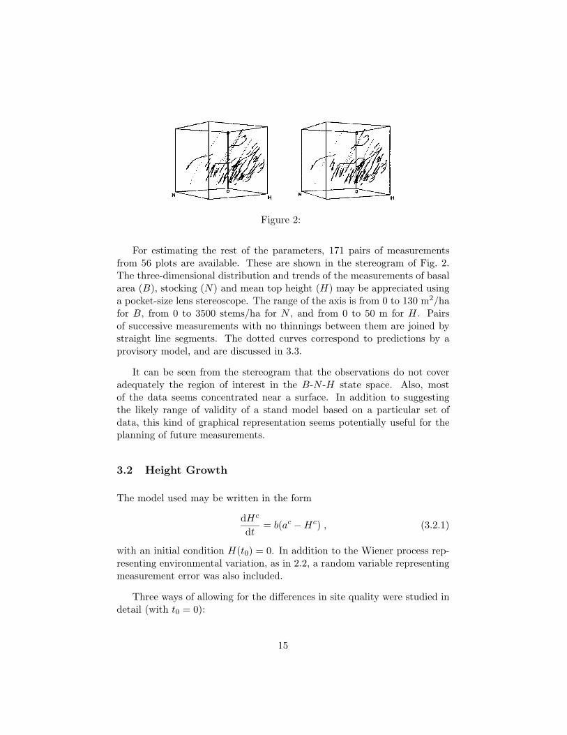
Figure 2:

For estimating the rest of the parameters, 171 pairs of measurementsfrom 56 plots are available. These are shown in the stereogram of Fig. 2.The three-dimensional distribution and trends of the measurements of basalarea (B), stocking (N) and mean top height (H) may be appreciated usinga pocket-size lens stereoscope. The range of the axis is from 0 to 130 m2/hafor B, from 0 to 3500 stems/ha for N , and from 0 to 50 m for H. Pairsof successive measurements with no thinnings between them are joined bystraight line segments. The dotted curves correspond to predictions by aprovisory model, and are discussed in 3.3.

It can be seen from the stereogram that the observations do not coveradequately the region of interest in the B-N -H state space. Also, mostof the data seems concentrated near a surface. In addition to suggestingthe likely range of validity of a stand model based on a particular set ofdata, this kind of graphical representation seems potentially useful for theplanning of future measurements.

3.2 Height Growth

The model used may be written in the form

dHc

dt= b(ac − Hc) , (3.2.1)

with an initial condition H(t0) = 0. In addition to the Wiener process rep-resenting environmental variation, as in 2.2, a random variable representingmeasurement error was also included.

Three ways of allowing for the differences in site quality were studied indetail (with t0 = 0):

15

(a) Parameters a and c were forced to be the same for every plot, and bfree to take a different value for each plot. This produces site indexcurves with a common upper asymptote (the asymptote is a).

(b) Parameters b and c the same for every plot, and a free. This producesanamorphic site index curves.

(c) Parameters a and b related by a = α + βS, with α, β and c commonfor all plots. S is the predicted height at age 20 years for each plot.and involves the free parameter b. This covers (a) and (b) as partic-ular cases (β = 0 and α = 0, respectively), at the cost of one extraparameter.

The “measurement” variance was allowed to take different values for eachof the plots, and the “environmental” variance was taken as proportionalto b, with the same proportionality constant for all plots. No appreciableimprovements were observed when t0 was allowed to take values differentfrom zero.

The following guides may be used to compare models in terms of the like-lihood function. Edwards (1972) considers that a difference of about twounits in the log-likelihood might be taken as “significant”. When compar-ing models with different numbers of parameters, Akaike (1975) and Stone(1977) suggest subtracting one unit for each additional parameter. Only dif-ferences in the log-likelihood matter; the exact values are largely irrelevant.

The following results were obtained for each of the models:

(a) Log-likelihood = 374.6a = 74.8c = 0.783

(b) Log-likelihood = 377.3b = 0.0267c = 0.775

(c) Log-likelihood = 377.9α = -46.3β = 5.08c = 0.774

There are no large differences in goodness of fit between the three models,although the data gives slightly better support to hypothesis (b). Graphical

16

comparison of the height-age curves shows little practical differences up tothe age of 30 years. Over 30 years the three models tend to diverge for lowand for high site indices. This suggests that the data do not define well thetrends in those regions (see Fig. 1), and any of the models must be regardedas unreliable for old stands in extreme sites.

Model (a) was selected, since it greatly simplifies the development of therest of the stand model. The resultant site index curves are shown in Figure1 (heights and site indices are in metres). These curves agree closely withthose obtained by Burkhart and Tennent (1978) using a different approach.

3.3 Full Model

Basal area, stocking and mean top height were adopted as the state variables.Three state variables is certainly a minimum for a satisfactory stand model(Garcia, 1968, 1974). As mentioned in 2.1, it might be desirable to add thegreen crown level and perhaps other variables. The green crown level mightimprove the performance of the model when heavy thinning or pruning areinvolved, and also improve the estimation of outputs by explaining part ofthe variation in log quality and in stem form. However, only a small part ofthe permanent sample plots available include measurements of crown level.It seems better at this stage to use the simpler three-dimensional state vectorand to assess the need for adjustments later (see 3.4).

A problem in implementing the model is to decide in what form the siteindex should enter in it. A convenient assumption is that the trajectories fol-lowed by stands in the state space (Fig. 2) do not depend on site index, onlythe speed of movement along a trajectory depending on it. In other words,the effect of the site index is a change in the time scale. Similar-assumptionshave often been used in forestry, for example in Beekhuis (1966). The modelof Elliott and Goulding (1976) does not make this assumption, but even so,the predicted trajectories differ remarkably little among site indices. Itseems useful to adopt this as a working hypothesis and to check it later atthe validation stage.

The height growth model with common asymptotes is compatible withthe time-scaling effect hypothesis, and this is the main reason why it wasselected. In terms of the stand model (2.3.2), the hypothesis implies thatonly the eigenvalues of A are functions of the site index; all the other pa-rameters are constants. Also, the eigenvalues depend on site index through

17

a proportionality factor which is the same for all the eigenvalues. An easyway of handling the effect of the site index when fitting the model is thento multiply the age by this factor, which can be taken as λ3. λ3 is the sameas −b in 3.2, and is a known function of the site index for each plot.

Two algorithms were tried for maximising the log-likelihood: a quasi-Newton procedure using finite difference approximations for the derivatives,coded in Algol (Lill, 1970), and a Fortran implementation of Nelder andMead’s (1965) Simplex method (O’Neill, 1971). Both algorithms were cho-sen mainly because they do not require derivatives and were readily avail-able. Quasi-Newton procedures (also known as Davidon-type or variable-metric methods) are usually very efficient, with good rates of convergence,specially near the optimum. The Simplex procedure is more robust, oftensucceeding with difficult functions when other methods fail, but it is gener-ally regarded as slower, specially when the number of variables is large.

Attempts using Lill’s program failed repeatedly, with the procedure ex-iting after a few iterations without reaching an optimum. It was foundlater that it also fails in the some way with a simple test function, for somestarting points. No errors have been detected in the transcription from thepublication, but some misprint is suspected.

With the Simplex method a rapid initial improvement in the functionvalue was generally obtained, but convergence was extremely slow after-wards. Several attempts with different starting points using the full function(2.3.10) (20 variables) were discontinued because of slow convergence.

Somewhat better results were obtained with a stage-wise approach, assuggested at the end of 2.3. First, some values were selected for C, andinitial estimates for the other parameters were obtained by linear regressionwith finite-difference approximations. Then the optimisation procedure wasapplied using (2.3.12). In addition, in this second stage the matrix A was alsorestricted to be diagonal (which implies P = I) . This reduces the number ofvariables (parameters) to 10. Much better values of the log-likelihood thanbefore were obtained, but still convergence was not complete after severalthousand function evaluations. In a third stage, the constraint P = I waslifted, increasing the number of variables to 14, and the optimisation wasrestarted. The computation was discontinued after about 6000 functionevaluations, with the log-likelihood still decreasing at a very slow but roughlylinear rate.

This seems to confirm the slow ultimate convergence of the Simplex

18

method for functions of many variables. It is hoped that the use of otherquasi-Newton procedures will produce much better results. The computingtime on the ICL 2980 computer, with the full 20-variables function (2.3.10),is approximately 1.3 minutes per thousand function evaluations, for our sam-ple of 171 observation pairs. The total optimisation time may be expectedto be roughly proportional to the number of observations.

Although their discrepancy from the M.L. estimates is unknown, thebest parameter values obtained until now way be used to illustrate somecharacteristics of the model and possible methods of validation.

According to the concepts explained in 2.1 and 2.2, the model defines afield of velocities and a set of trajectories or flow-lines that fill completely theB-N -H state space. Through each point in this space, passes one and onlyone trajectory. No matter how a stand arrives to a point, it will follow thecorresponding trajectory until the next thinning. The effect of a thinningis a jump from one trajectory onto another. Observing the paths followedby stands in Figure 2, and considering the natural variability in this kind ofdata, these ideas do not seem entirely unrealistic.

A few trajectories predicted by the provisional model are included inFigure 2 as dotted curves. Each dot corresponds to one year growth forsite index 23. They do not seem too unreasonable, except for the higherdensities where one would expect heavier mortality. It might be observedthat there are very few plots in this region, and their trends are somewhaterratic.

Figure 3 represents two “cuts” through Figure 2, showing projections ofthe predicted velocity field at the planes H = 15 m and H = 30 m. The linesegments represent the directions in which stands at different points in thestate space would move. The length of the line segments corresponds to two-years’ growth on site 23. 0f course, reliable prediction is only possible withinthe area covered by the data. In particular, the increases in stocking shownfor the region of high stocking and low basal area are clearly impossible. Thepossibility that predictions would be improved by constraining the model tofeasible behaviour over all or part of the state space is still an open question.

19

Figure 3:

3.4 Validation

The discussion is limited to demonstrating a particular technique whichseems useful for assessing results obtained with models of the type describedin 2.2. For other validation methods which could also be used see Goulding(1978).

From (2.3.6), note that the M.L.E. for the logarithms of the absolutevalues of the zi are linear functions of time. We might then plot the ln |zi|computed from the data versus t, and look for systematic deviations fromlinearity.

It seems better, instead, to plot ln |zi| vs. ln |zj | for all the combinations

20

of i and j. These relationships still tend to straight lines, and it might beexpected that large part of the variation due to year-to-year differences ingrowth rates would be eliminated. In addition, with the particular assump-tion on the effect of site index made in 3.3, the slopes λi/λj must be thesame for all plots.

The data have been plotted in this way in Figure 4. Successive mea-surements with no thinnings between have been joined with straight linesegments. The same data is also shown three-dimensionally in the stere-ogram in Figure 5. In addition, in Figure 4 the plots have been groupedin three site index classes and distinguished with different line types: siteindices less than 22.5 with dotted lines, 22.5 to 23.5 with dashed lines, andover 23.5 with continuous lines. The small triangles mark measurementsimmediately following a thinning.

In general, the trajectories seem to follow reasonably well the theoreticalpattern of parallel straight lines. Some notable exceptions correspond to theplots with high density and erratic mortality already mentioned. There is noevidence of systematic differences in slope or in curvature between site indexclasses; the site index hypothesis seems satisfactory. The graphs also givesome information on the effect of thinnings. In most cases the trajectoriesimmediately after thinnings (triangles) are not appreciably different fromthose for other measurements, but there are several instances in which clearlythis is not so. Identification of these measurements and examination of theplot records might show if there is anything special about them, if theycorrespond to exceptionally heavy thinnings or perhaps high prunings, andindicate if adjustments to the model become necessary.

Notes

Section 2.1

System Theory has been developing as an independent discipline duringthe 1970s and late ’60s, embracing and extending what was the “state spaceapproach” in the Control Theory of the ’60s. In turn, Control Theory derivedmainly from part of what was called Cybernetics in the ’50s. For furtherdetails the following sequence of readings can be recommended:

Garcia (1974), Chapter 1 of Bellman and Kalaba (1965), Chapter 1 of

21

Figure 4:22

Figure 5:

Wiberg (1971), and Padulo and Arbib (1974). Patten (1971) and Bellmanand Kalaba (1960) are also useful.

Many efforts in modelling stands have suffered from failures in selectingappropriate states and transition functions. The model of Beekhuis (1966)is remarkable in being perhaps the first model for managed stands with asound structure. It had an adequate state vector, and its transition function“almost” satisfied the semigroup property. The same can be said of manylater models (e.g., Elliott and Goulding, 1976), but some ones with seriousdeficiencies continue to be produced. It is felt that a better appreciationof system-theoretic ideas might help to clarify the issues involved (Garcia,1968, 1974).

The discussion of systems in section 2.1 has actually been restricted totime-invariant systems. This is not considered important, since time-varyingsystems, that is those whose behaviour depends explicitly on time, can beformulated as time-invariant ones by including time as an additional statevariable.

Section 2.2

What we have called the Bertalanffy model is frequently referred to as theChapman-Richards model in the forestry literature. It seems to have beenfirst proposed by Bertalanffy (1949, 1957), and later its properties exten-sively analysed by Richards (1959). The usual reference for Chapman isChapman (1961), where the model is used but nothing new about it isadded.

23

A useful reference for linear differential systems is Wiberg (1971).

The notation for the stochastic differential equation (2.2.8) follows Er-ickson (1971). Strictly speaking it might be considered as incorrect, becausethe Wiener process is not differentiable. More correct and more usual (forstochastic differential equations) would be

dxC = (AxC + b) dt + B dw

(Gihman and Skorohod, 1972). However, (2.2.8) has been used because itlooks more familiar for most people.

Section 2.3

Instead of permanent sample plot data, stem analysis could be used if someway of estimating mortality is available. A combination of both types ofdata is also possible.

Many authors define a likelihood function only up to a factor of propor-tionality (which can depend on the data).

A maximum of the likelihood function may do not exist. In practice thisusually indicates an inadequate formulation of the model. More troublesomeis the possibility of local maxima (see Chambers, 1973).

All the results of sections 2.2 and 2.3 are valid for state vectors with anynumber of components.

It may be sometimes desirable to impose constraints on some of theparameters when maximising the log-likelihood. Many constraints can easilybe implemented by transformations of parameters. For example, parametersconstrained to be non-negative may be replaced by the square of a newparameter. In fact, any constraint can be enforced through transformations,possibly at the cost of adding new variables. Alternatively, a NonlinearProgramming algorithm may be used.

Section 3.2

The guides suggested for comparing models on the basis of likelihoods mustbe regarded only as a rough aid to intuition, and used in conjunction with

24

other knowledge or sources of evidence, if possible. In general, the wholeproblem of Statistical Inference tends to be an ill-defined one. See Barnett(1973) for a good review of some of the issues involved.

An unexpected result was that in all cases the estimate for the “environ-mental” variance was zero. However, the estimated correlations between theestimates for the two variances were fairly high. This suggests that the datadoes not allow a reliable partition of the variation into “environmental” and“measurement” components.

Section 3.3

A practical way of simulating the development of a stand with the model isas follows. First, compute the one-year transition matrix corresponding tothe appropriate site index as

T = P−1eΛP ,

and the vector h = a−Ta. Compute y(t0) = xC for the initial state vectorx = x(t0). Then project forward by repeatedly applying the recursion

y(t + 1) = Ty(t) + h .

The states are recovered through x = yC−1. Note that the zeros in the

matrices allow for some simplification in the computations.

It seems evident that to develop a reliable stand model a fair amount ofdata, well distributed over the state space, is required. A possible strategyfor developing local models for regions where the data are inadequate mightbe the use of “adapted” models. This means that part of the parameters,for example the matrix C and perhaps also P , are taken from other regionwhere a good model is already available. Then the optimization, possiblyusing the simplified log-likelihood given by (2.3.12), is carried out over theremaining parameters using the local data.

References

Akaike, H. 1973: Information Theory and an extension of the maximum like-lihood principle. In: Petrov, B.N. and Czaki, G. (eds), 2nd InternationalSymposium on Information Theory. Akademia Kiado, Budapest.

25

Barnett, V. 1973: Comparative Statistical Inference. Wiley, London.

Beekhuis, J. 1966: Prediction of yield and increment in Pinus radiata standsin New Zealand. Technical Paper No. 49, Forest Research Institute, N. Z.Forest Service.

Bellman, R. and Kalaba, R. 1960: Dynamic Programming and AdaptiveProcesses: Mathematical foundation. IRE Transactions on AutomaticControl, AC–5, 5–10. (Reprinted in: Bellman, R. and Kalaba, R. (eds)Selected papers on mathematical trends in Control Theory. Dover, NewYork, 1964).

Bellman, R. and Kalaba, R. 1965: Dynamic Programming and modern Con-trol Theory. Academic Press, New York.

Bertalanffy, L. von 1949: Problems of organic growth. Nature, 163 : 156–158.

Bertalanffy, L. von 1957: Quantitative laws in metabolism and growth. TheQuart. Rev. Biol., 32 : 217–231.

Burkhart, H.B. and Tennent, R.B. 1978: Site index equations for Radiatapine in New Zealand. N .Z. J. For. Sci. 7 : 408–416.

Chambers, J. M. 1973: Fitting nonlinear models: Numerical techniques.Biometrika, 60 : 1–13.

Chapman, D. G. 1961: Statistical problems in population dynamics. Proc.Fourth Berkeley Symp. Math. Stat. and Prob. University of CaliforniaPress, Berkeley.

Edwards, A. W. F. 1972: Likelihood. Cambridge Univ. Press.

Elliott, D. A. and Goulding, C .J. 1976: The Kaingaroa growth model forRadiata pine and its implications for maximum volume production (ab-stract). N. Z. J. For. Sci., 6 : 187.

Erickson, R. V. 1971: Constant coefficient linear differential equations drivenby white noise. Ann. Math. Statist., 42 : 820–823.

Garcia V., O. 1968: Problemas y modelos en el manejo de las plantacionesforestales. U. of Chile, Esc. Ing. Forestal. (thesis).

26

Garcia V., O. 1974: Sobre modelos matematicos de rodal. Informe Tecnico48, Instituto Forestal, Chile (English translation available at the F.R.I.library).

Gihman, I. J. and Skorohod, A. V. 1972: Stochastic Differential Equations.Springer-Verlag, New York.

Goldberg, S. 1958: Introduction to Difference Equations. Wiley, New York.

Goulding, C. J. and Shirley, J .W. 1978: A method to predict the yield of logassortments for long term planning. (Paper presented at this Symposium).

Goulding, C. J. 1978: The validation of growth models used in forest men-suration. (Submitted for publication to the N. Z. J. of Forestry).

Jackson, D. S., Gifford, H. H. and Chittenden, J. 1976: Environmentalvariables influencing the growth of Radiata pine: (2) Effects of Seasonaldraught on height and diameter increment. N. Z. J. For. Sci. 5 : 265–286.

Jacoby, S. L. S., Kowalik, J. S. and Pizzo, J .T. 1972: Iterative methods fornonlinear optimization problems. Prentice-Hall, Englewood Cliffs, N.J.

Kalman, R. E., Falb, P. L. and Arbib, M. A. 1969: Topics in MathematicalSystem Theory. McGraw-Hill, New York.

Karlin, S. 1966: A first course in Stochastic Processes. Academic Press, NewYork.

Lill, S. A. 1970: Algorithm 46: A modified Davidon method for findingthe minimum of a function using difference approximation for derivatives.Computer J., 13 : 111–113 (and corrections in 14, 106).

Martin, R. S., Peters, G. and Wilkinson, J. H. 1971: Symmetric decompo-sition of a positive definite matrix. In: Wilkinson, J. H. and Reinsch, C.(eds). Linear Algebra – Handbook for Automatic Computation, VolumeII Springer - Verlag, Berlin.

Miller, K. S. 1968: Linear Difference Equations. Benjamin, New York.

Murray, W. 1972 (ed). Numerical methods for unconstrained optimization.Academic Press, London.

Nelder, J. A. and Mead, R. 1965: A simplex method for function minimiza-tion. Computer J., 7 : 308–313.

27

O’Neill, R. 1971: Algorithm AS47 – Function minimization using a simplexprocedure. Appl. Statist., 20 : 338–345 (corrections and changes in 23,250–252 and 25, 97).

Padulo, L. and Arbib, M. A. 1974: System Theory. Hemisphere Pub. Co.,Washington, D.C.

Patten, B. C. 1971: A primer for ecological modelling and simulation withanalog and digital computers. In: Patten, B. C. (ed) System Analysis andsimulation in Ecology. Academic Press, New York.

Richards, F. J. 1959: A flexible growth function for empirical use. J. Expt.Botany, 10 : 290–300.

Stone, M. 1977: An asymptotic equivalence of choice of model by cross-validation and Akaike’s criterion. J. R. Statist. Soc., B, 39 : 44–47.

Tomlinson, A. I. 1976: Short period fluctuations of New Zealand rainfall. N.Z. J. of Science 19 : 149–161.

Wiberg, D. M. 1971: State space and linear systems. Shaum’s Outline Series,McGraw-Hill, New York.

Zacks, S. 1971: The theory of Statistical Inference. Wiley, New York.

Zadeh, L. A. 1969: The concepts of system, aggregate, and state in systemtheory. In: Zadeh, L. A. and Polak, E. (eds). System Theory. McGraw-Hill, New York.

28