Modelling spatial patterns of distribution and abundance of mussel

Statistics & Operations Research TransactionsSORT 34 (1) January-June 2010, 67-78

Statistics &Operations Research

Transactionsc© Institut d’Estadıstica de [email protected]: 1696-2281

www.idescat.net/sort

Modelling spatial patterns of distribution andabundance of mussel seed using Structured

Additive Regression models

Marıa P. Pata1, Marıa Xose Rodrıguez-Alvarez2,3, Vicente Lustres-Perez1

Eugenio Fernandez-Pulpeiro1, Carmen Cadarso-Suarez2,3

Abstract

As mussel farming depends on sources of natural mussel seed, knowledge of factors is requiredto regulate both the spatial distribution and abundance of this resource. These spatial patternswere modelled using Bayesian STructured Additive Regression (STAR) models for categoricaldata, based on a mixed-model representation. We used Bayesian penalized splines for modellingthe continuous covariate effects and a Markov random field prior for estimating the spatial effects.

MSC: 62F15, 62G08, 62P12, 92D40.

Keywords: Mussel seed, Bayesian structured additive regression (STAR) models, spatial effects,Bayesian P-splines.

1. Introduction

Knowledge of spatial patterns of distribution and abundance of species is essentialin order to understand the ecological processes that have generated such processes(Underwood, Chapman and Connell (2000)). In the case of marine resources, knowledgeof these patterns is of crucial interest.

Mussel farming is widely developed along most of Galicia’s Atlantic coastline, andindeed this region is the largest producer in Europe (200,000 MT/year). As mussel

1 Departamento de Zoologıa y Antropologıa Fısica, Universidade de Santiago de Compostela (USC), Spain.2 Unidad de Bioestadıstica, Departamento de Estadıstica e Investigacion Operativa, USC, Spain.3 Instituto de Investigacion Sanitaria de Santiago (IDIS), Santiago de Compostela, Spain.Received: November 2009Accepted: May 2010

68 Modelling spatial patterns of distribution and abundance of mussel seed using STAR models

farming depends on natural mussel seed resources, knowledge of its distribution andabundance is fundamental to prevent depletion of natural populations.

In ecology, Generalized Linear Models (GLM, McCullagh and Nelder (1997))are the most widely used statistical models to assess relationships between speciesdistribution and environment. In recent years, however, biomedical researchers haveshown a great interest in the use of Generalized Additive Models (GAM, Hastieand Tibshirani (1990); Wood (2006)), due the latter’s ability to cover the complexnon-linear effects had by continuous covariates on the outcome of interest. Recentapplications of GAMs in ecology (see, for instance, Austin (2002), Austin (2007),Guisan, Edwards and Hastie (2002)) show that GAM regression models are useful toolsfor analysing relationships between species’ distributions and their environment. Yet,spatial autocorrelation often exists in the data because the sample points are close to oneanother and subject to the same environmental factors (see Kneib, Muller and Hothorn(2008)). Since spatial correlation is difficult to handle within a GAM framework, a moregeneral regression model is thus called for.

Accordingly, this study modelled the spatial distribution of mussel seed within aBayesian STructured Additive Regression Model (STAR, Fahrmeir and Lang (2001))framework. Inference was based on a mixed-model representation (Kneib and Fahrmeir(2006)). The use of STAR models affords several advantages when analysing spatialdata, including, among others, the possibility of incorporating: (a) flexible forms ofthe effects of continuous covariates, by using Bayesian P-splines (Eilers and Marx(1996), Lang and Brezger (2004)); (b) flexible spatial effects; and, (c) random effectsto explain the overdispersion caused by unobserved heterogeneity or the presence ofautocorrelation in spatial data (Fahrmeir and Lang (2001)). Models that enable smootheffects of continuous covariates and spatial effects with flexible forms to be incorporatedare known as geoadditive models (Kammann and Wand (2003)). In this paper, we useda geoadditive multicategorical regression model (Kneib and Fahrmeir (2006)), in whichthe response variable was assumed to follow a multinomial distribution.

The paper is structured as follows: the mussel seed data are introduced in Section 2;the statistical methodology is described in Section 3; the results from fitting the proposedSTAR models to mussel seed data are shown in Section 4; and the paper concludes witha Discussion Section.

2. The mussel seed data

This study was undertaken during spring tides at 62 sites along Galicia’s Atlanticseaboard, between 43◦21′ N, 8◦21′ W and 42◦44′ N, 9◦04′ W, from March to Septemberin 2005 and 2006.

At each site, a transect perpendicular to the coastline was placed in the intertidalzone. A sample quadrant (20×20 cm) was set at 50-centimetre intervals and thepercentage cover of mussel seed then measured. Information from a set of covariates

Marıa P. Pata et al. 69

was taken in order to explain the distribution pattern of the mussel seed. These covariateswere tidal height (in metres), percentage of pools, and positioning related to cardinalpoints divided into the following five categories: NN; NE; SE; SW; and NW.

For study purposes, the outcome of interest was percentage cover (from 5% upwards,in multiples of 5%). This variable was treated as categorical, and the following fourcategories were established:

Category 1: low abundance, [0% - 5%]. This was used as the reference category;Category 2: medium, (5% - 25%];Category 3: high, (25% - 50%];Category 4: very high, > 50%.

Within the STAR framework, several approaches can be used to analyse categoricalresponses, such as the multinomial model for nominal categories or the cumulative logitprobit models, among others, for ordered categories. Despite the fact that a better optionmight have been the cumulative model, we nevertheless chose to use a multinomialmodel in view of the biological interest that this option could afford.

All computations were performed using the BayesX package (Belitz et al. (2009)).

3. Statistical methodology: geoadditive multicategoricalregression model

In multicategorical data the response variable Y is observed in categories r ∈ (1, . . . ,k).Analysis of this type of data calls for an appropriate model to take into account theadditional information supplied by these categories (Boeck and Wilson (2004)). In thispaper, a multinomial logit model was considered, with the probability of the category rexpressed as follows:

P(Y = r|u) = π(r) = h(r)(η(1), . . . ,η(q)

)=

exp(η(r))

1+∑qs=1 exp

(η(s)) , r = 1, . . . ,q = k−1,

with k as reference category, and the linear predictor η(r) = u′α(r), depending oncovariates u and category-specific vector of regression coeficients α(r). It is possibleto obtain the general multinomial model

π= h(η) , η=Vγ,

by defining the design matrix

V =

⎛⎜⎝υ

′1...υ

′q

⎞⎟⎠=

⎛⎜⎝

u′

0. . .

0 u′

⎞⎟⎠


and the overall vector of regression parameters (Kneib (2006); Kneib and Fahrmeir(2006))

γ=(α(1), . . . ,α(q)

).

To take into account the spatial information for each unit (administrative areas in ourexample), the following geoadditive multicategorical model (defined by the geoadditivepredictor) is then considered

η(r)i = u

′iα

(r) + f (r)1 (xi1)+ . . .+ f (r)l (xil)+ f (r)spat (si) ,

where f (r)1 , . . . , f (r)l are unknown smooth functions of the covariates x1, . . . , xl , and

f (r)spat is the non-linear effect of spatial index si ∈ {1, . . . , S} (administrative area in ourexample).

This specification of the model allows for flexible incorporation of non-linear ef-fects of continuous covariates and spatial effects. Furthermore, the different types ofcovariates are considered in a unified framework (Fahrmeir and Lang (2001); Kneib andFahrmeir (2006)).

Since spatial correlation and/or heterogeneity due to unobserved spatially varyingcovariates are usually present in spatial data, it seems appropiate for the spatial effectto be broken down into a spatially correlated part (structured part: fstr) and a spatiallyuncorrelated part (unstructured part: funstr):

f (r)spat (s) = f (r)str (s)+ f (r)unstr (s) .

This representation of the spatial effects makes it possible to distinguish between the twokinds of unobserved covariates, namely, those that display a strong spatial structure andthose that are present locally (Besag, York and Mollie (1991); Fahrmeir et al. (2003)).

To estimate smooth effect functions and model parameters, an empirical Bayesianapproach based on mixed model representation is used. Assigning appropriate priorsfor parameters and functions is crucial. For the fixed effects parameter γ, diffuse priorsp(γ) ∝ const are asssumed.

For specifying smoothness priors for continous covariates, a Bayesian version of theP-splines approach of Eilers and Marx (1996) is used (Lang and Brezger (2004)). Thisapproach assumes that the effect f of a covariate x can be approximated by a polinomialspline of degree l defined on a set of equally spaced knots xmin = ξ0 < ξ1 < .. . < ξr−1 <

ξr = xmax. This can be written in terms of a linear combination of Mj = r j + l j B-splinebasis functions

f j (x) =Mj

∑m=1

β jmBm (x) ,

where β j is the vector of the unknown regression coefficients.


The main problem when dealing with these splines lies in the selection of the numberof knots and their placement. The idea of P-splines is to select a generous number ofknots and define a roughness penalty on adjacent regression coefficients to regularisethe problem and avoid overfitting (Eilers and Marx (1996)). In the frequentist approach,first- or second-order differences are usually used. From a Bayesian perspective, theseare replaced by their stochastic analogues, namely, first-or second-order random walks.For the purposes of this study, we used second-order random walks for the regressioncoefficients, defined as

β jm = 2β j,m−1 −β j,m−2 +u jm,

with Gaussian errors u jm ∼ N(0,τ2

j

). (Lang and Brezger (2004)). The variance param-

eter τ2j controls the amount of smoothnes.

Since the spatial locations are clustered in connected geographical regions, a MarkovRandom Field prior (Besag et al. (1991)) is selected for the structured spatial effects.This spatial smoothness prior is defined by

{fstr(s)| fstr(s′); s �= s′,τ2

}∼ N

(∑s∈δs

fstr(s′)Ns

,τ2

Ns

),

where Ns is the number of adjacent sites, s ∈ δs ndicates that site s′is neighbour of site

s, that is, they share a common boundary (Fahrmeir and Lang (2001), Kneib (2006)).The unstructured spatial effects are assumed to be i.i.d. random effects funstr(s) ∼

N(0,τ2

)(Fahrmeir et al. (2004); Kneib and Fahrmeir 2006).

Inference is performed with empirical Bayes (EB) posterior analysis based on gen-eralized linear mixed model (GLMM) methodology, once an appropiate reparameteri-zation of the regression terms is given. For empirical Bayes inference, the variances τ2

j

are considered as unknown constants to be estimated from their marginal likelihood.Based on the GLMM approach regression and variance parameters can be estimatedusing iteratively weighted least squares (IWLS) and (approximate) restricted maximumlikelihood (REML) developed for GLMM’s. For detailed description of the estimationprocedure see Fahrmeir et al. (2004) and Kneib and Fahrmeir (2006).

4. Results

To analyse the spatial distribution of mussel seed with respect to the relevant explanatoryvariables, a geoadditive multinomial logit model was applied. The parametric effects ofsites’ positioning in terms of cardinal points as well as the smooth effects of tidal heightand percentage of pools were included in the model.


A summary of the estimated effects of site positioning for each category is shownin Table 1. The category with the highest frequency, SW, was chosen as the referencecategory. As can be seen from Table 1, the results were only significant for Category2 (mussel seed abundance of 5%-25%), and as NN-, NE- and NW-positioning of sitesreduced the presence of this category, SW-positioning was therefore the best for thepresence of Category 2.

Table 1: Estimates, standard deviations (S.D) and 95% credible confidence interval for the fixed effects.Category 1 (< 5%) is taken as reference category.

Estimated effects S.D. 95%CI

Category 2 (5%-25%]

NN −1.73 0.662 −3.02 −0.43NE −0.86 0.179 −1.21 −0.51SE −0.17 0.280 −0.72 0.37NW −0.36 0.161 −0.68 −0.04

Category 3 (25%-50%]

NN −0.04 0.435 −0.86 0.54NE −0.03 0.365 −0.74 0.68SE 0.41 0.441 −0.44 0.44NW 0.06 0.251 −0.42 0.25

Category 4 > 50

NN −0.49 0.687 −1.04 0.06NE −0.09 0.769 −1.60 1.41SE 0.36 0.784 −1.16 1.90NW 0.44 0.553 −0.64 1.53

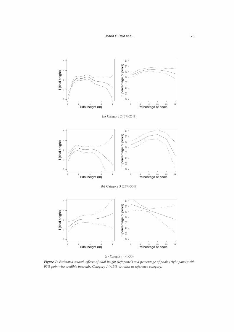
The estimated smooth effects of tidal height and percentage of pools on the presenceof mussel seed are shown in Figure 1. As can be seen, these are complex nonlineareffects. Hence, the use of purely linear models to describe such data could lead toestimations and, by extension, conclusions that were erroneous. STAR models enableflexible forms of the effects of continuous covariates to be incorporated in the responseand better knowledge of the biological process so obtained.

The effect of tidal height appeared to be similar for the above three categories inthe initial metres, with a much more pronounced shape for Category 2. The functionincreased until a tidal height of about two metres, and then decreased from 4 metres. Itseems that the most suitable tidal heights for the presence of mussel seed range from 2to 4 metres, particularly for Category 2. For Category 3, tidal height appeared to haveno effect from a height of about 2 metres.

The effects of percentage of pools are depicted in the right panels of Figure 1. For thepresence of Categories 2 and 3, which plotted similar patterns, sites with 15% to 20%of pools would seem to be more suitable. The presence of these categories decreased


Tidal height (m)

f (tid

al h

eigh

t)−

4−

20

24

0 2 4 6 8

Percentage of pools

f (pe

rcen

tage

of p

ools

)−

2.5

−2.

0−

1.5

−1.

0−

0.5

0.0

0.5

1.0

5 10 15 20 25 30

(a) Category 2 (5%-25%]

Tidal height (m)

f (tid

al h

eigh

t)−

4−

20

24

0 2 4 6 8

Percentage of pools

f (pe

rcen

tage

of p

ools

)−

2.5

−2.

0−

1.5

−1.

0−

0.5

0.0

0.5

1.0

5 10 15 20 25 30

(b) Category 3 (25%-50%]

Tidal height (m)

f (tid

al h

eigh

t)−

4−

20

24

0 2 4 6 8

Percentage of pools

f (pe

rcen

tage

of p

ools

)−

2.5

−2.

0−

1.5

−1.

0−

0.5

0.0

0.5

1.0

5 10 15 20 25 30

(c) Category 4 (>50)

Figure 1: Estimated smooth effects of tidal height (left panel) and percentage of pools (right panel),with95% pointwise credible intervals. Category 1 (<5%) is taken as reference category.


thereafter but posterior probabilities were non-significant above 20%. For Category 4(very high abundance), in contrast, the presence of mussel seed decreased linearly withpercentage of pools.

Figure 2 displays the spatial effects on a grey scale, after controlling for the covari-ates: white colour refers to a positive spatial effect signifying higher abundance of thecategory, while dark colour refers to a negative effect signifying lower abundance. Thesignificance of the structured spatial effects are shown in the third column of Figure2, with black areas indicating strictly negative credible intervals, white ones indicatingstrictly positive, and grey areas indicating no effect. In cases where the structured spatialeffects proved non-significant, the map of posterior probabilities is not shown.

As can be seen from the maps (Figure 2, first row), the structured spatial effectsfor Categories 3 and 4 displayed a clear regional pattern but were not significant forCategory 2. There is a descending south-north gradient, with southern regions appearingto be more appropriate and northern areas unsuitable for the presence of mussel seed.These results seem to be plausible because the northern areas are extremely exposed andsteep, and even the nature of the substrate is less suitable for settlement and, by the sametoken, a higher abundance of mussel seed.

In the maps of unstructured effects (Figure 2, second row), the dashed areas denoteregions in which unstructured effects are not estimated. No clear pattern in unstructuredeffects is displayed in these maps and, compared to the structured effects, the localeffects were smaller. Moreover, the posterior probabilities (maps not shown) indicatethat no region has a significant effect on response.

5. Conclusions

This study proposes a novel application of STAR models to the field of marine resources.The use of geoadditive multicategorical models for mussel seed data demonstrates thatthese models can be very useful tools for fitting this type of biological data. STARmodels enable flexible non-linear effects of covariates as well spatial effects to be in-corporated. Moreover, since spatial effects can be split into spatially correlated and un-correlated parts, it becomes possible to distinguish between unobserved covariates thatdisplay a strong spatial structure and those that are only present locally. Our data re-vealed marked, downward, south-north spatial pattern. However, since the unstructuredeffects were not significant, the distribution of the mussel seed would not seem to beaffected by locally present covariates.

As pointed out in Section 2 above, though the response variable was treated asnominal (with multinomial distribution) in this study, this outcome could also beconsidered ordinal, in which case other STAR models, such as cumulative probit/logitmodels, could be used in our application. Future extensions of our work include astatistical comparison of categorical versus cumulative models for fitting mussel seeddistribution.


0 00 −0.73 0.620

(a) Category 2 ( 5%-25% ]

−1.23 1.530 −0.43 0.690

(b) Category 3 ( 25%-50% ]

−1.32 0.970 −0.32 0.430

(c) Category 4 ( >50%)

Figure 2: From left to right, averages estimates of the structured spatial effects (first column), unstructuredspatial effects (second column) and posterior probabilities (third column). Category 1 (<5%) is taken asreference category. For category 2 the map of posterior probabilities is not shown since the structuredspatial effects proved non-significant.


Finally, an additional advantage of using STAR models for fitting ecological data liesin the flexibility of incorporating temporal effects in a simple manner, something thatmakes it possible to offer flexible spatio-temporal models, which are of great interest inmany biomedical fields.

Acknowledgements

The authors would like to express their gratitude for the support received in the form ofthe Spanish MEC Grant MTM2008-01603 and the Galician Regional Authority (Xuntade Galicia) projects INCITE08PXIB208113PR and 07MMA001200PR. We are alsograteful to the referee for her/his valuable comments and suggestions, which servedto make a substancial improvement to this paper.

References

Austin, M. P. (2002). Spatial prediction of species distribution: an interface between ecological theory andstatistical modelling. Ecological Modelling, 157, 101-118.

Austin, M. P. (2007). Species distribution models and ecological theory: a critical assessment and somepossible new approaches. Ecological Modelling, Review, 200, 1-19.

Belitz, C., Brezger, A., Kneib, T. and Lang, S. (2009): BayesX - Software for Bayesian inference in struc-tured additive regression models. Version 2.0.

Besag, J., York, J. and Mollie, A. (1991). Bayesian image restoration with two applications in spatial statis-tics (with discussion). Annals of the Institute of Statistical Mathematics, 43, 1-59.

Boeck, P. and Wilson, M. eds. (2006). Explanatory Item Response Models: A Generalized Linear and Non-linear Approach. Springer, New York.

Eilers, P. H. C. and Marx, B. D. (1996). Flexible smoothing using B-splines and penalties (with commentsand rejoinder). Statistical Science, 11, 89-121.

Fahrmeir, L. and Lang, S. (2001). Bayesian inference for generalized additive models based on Markovrandom field priors. Applied Statistics, 50 (2), 201-220.

Fahrmeir, L., Kneib, T. and Lang, S. (2004). Penalized structured additive regression for space-time data: aBayesian perspective. Statistica Sinica, 14, 731-761.

Guisan, A., Edwards, T. C. and Hastie, T. (2002). Generalized linear and generalized additive models instudies of species distributions: setting the scene. Ecological Modelling, 157, 89-100.

Kammann, E. E. and Wand, M. P. (2003). Geoadditive models. Journal of the Royal Statistical Society C,52, 1-18.

Kneib, T. (2006). Mixed model based inference in structured additive regression. PhD thesis, Dr.Hut-Verlag.Kneib, T. and Fahrmeir, L. (2006). Structured additive regression for categorical space-time data: a mixed

model approach. Biometrics, 62, 109-118.Kneib, T., Muller, J. and Hothorn, T. (2008). Spatial smoothing techniques for the assessment of habitat

suitability. Environmental and Ecological Statistics, 15, 343-364.Lang, S. and Brezger, A. (2004). Bayesian P-splines. Journal of Computational and Graphical Statistics,

13, 183-212.McCullagh, P., Nelder, J. A. (1997). Generalized Linear Models, second ed. Chapman and Hall, London.


Underwood, A. J., Chapman, M. G. and Connell, S. D. (2000). Observation s in ecology: you can’t makeprogress on processes without understanding the patterns. Journal of Experimental Marine Biologyand Ecology, 250, 97-115.

Wood, S. N. (2006). Generalized additive models: an introduction with R. CRC Press, Boca Raton, FL.

Documents

Modelling spatial patterns of distribution and abundance of mussel