Journal of Mathematical Biology (2019) 78:815–835https://doi.org/10.1007/s00285-018-1293-z Mathematical Biology

Large scale patterns in mussel beds: stripes or spots?

Jamie J. R. Bennett1 · Jonathan A. Sherratt1

Received: 5 February 2018 / Revised: 13 June 2018 / Published online: 5 September 2018© The Author(s) 2018

AbstractAn aerial view of an intertidal mussel bed often reveals large scale striped patternsaligned perpendicular to the direction of the tide; dense bands ofmussels alternate peri-odically with near bare sediment. Experimental work led to the formulation of a setof coupled partial differential equations modelling a mussel–algae interaction, whichproved pivotal in explaining the phenomenon. The key class of model solutions to con-sider are one-dimensional periodic travelling waves (wavetrains) that encapsulate theabundance of peak and trough mussel densities observed in practice. These solutionsmay, or may not, be stable to small perturbations, and previous work has focused ondetermining the ecologically relevant (stable) wavetrain solutions in terms of modelparameters. The aim of this paper is to extend this analysis to two space dimensionsby considering the full stripe pattern solution in order to study the effect of transversetwo-dimensional perturbations—a more true to life problem. Using numerical con-tinuation techniques, we find that some striped patterns that were previously deemedstable via the consideration of the associated wavetrain solution, are in fact unstableto transverse two-dimensional perturbations; and numerical simulation of the modelshows that they break up to form regular spotted patterns. In particular, we show thatbreak up of stripes into spots is a consequence of low tidal flow rates. Our consider-ation of random algal movement via a dispersal term allows us to show that a higheralgal dispersal rate facilitates the formation of stripes at lower flow rates, but alsoencourages their break up into spots. We identify a novel hysteresis effect in musselbeds that is a consequence of transverse perturbations.

Jamie J. R. Bennett’s work was supported by The Maxwell Institute Graduate School in Analysis and ItsApplications, a Centre for Doctoral Training funded by the UK Engineering and Physical SciencesResearch Council (Grant EP/L016508/01), the Scottish Funding Council, Heriot-Watt University, and theUniversity of Edinburgh.

B Jamie J. R. Bennettjjb1@hw.ac.uk

Extended author information available on the last page of the article

123

816 J. J. R. Bennett, J. A. Sherratt

Keywords Mussels · Mussel–algae interaction · Activator-inhibitor ·Self-organisation · Pattern formation · Turing–Hopf bifurcation · Two-dimensionalstability · Tranverse perturbations

Mathematics Subject Classification 35Q92 · 35K57 · 35B36 · 35C07

1 Introduction

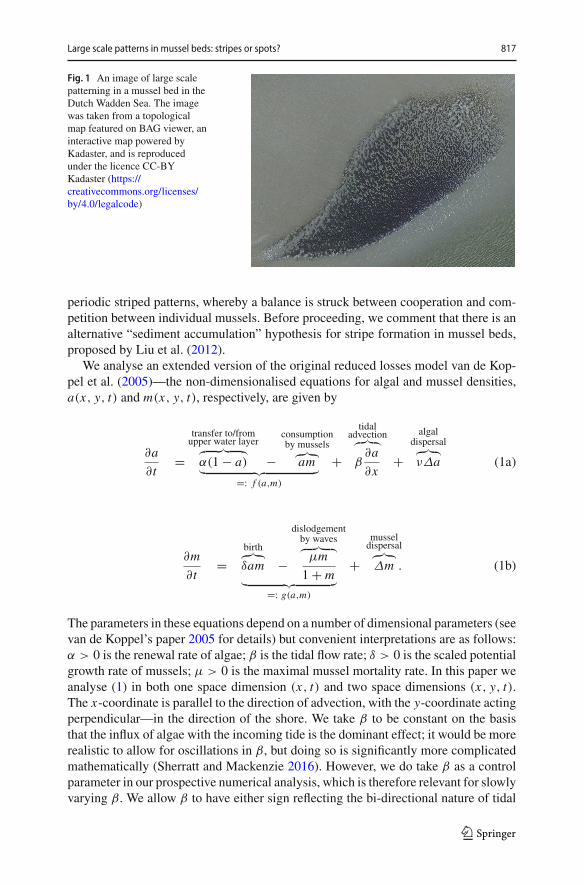
Blue mussels (Mytilus edulis) are often known as the common mussel because oftheir persistence in abundance across various intertidal regions. They usually playimportant roles in biodiverse ecosystems as major food sources for aquatic and terres-trial animals, and also form the foundations of many shallow water, benthic habitats.One important role is the circulation of nutrients via filter feeding—water is siphonedover the gills where suspended biomass, such as algae, enters the digestive system.The excrements provide nutrients for other marine animals, and bi-products (pseud-ofaeces) become a form of enriched sediment, thought to increase species diversity(Dame et al. 1991). A comprehensive overview of the blue mussel has been collatedin an online archive (Tyler-Walters 2008) by The Marine Biological Association. Theecological and agricultural significance of the blue mussel has prompted numerousempirical (Christensen et al. 2015; Dobretsov 1999; Capelle et al. 2014; Okamura1986; Hughes and Griffiths 1988; Guiñez and Castilla 1999), as well as mathematical(van de Koppel et al. 2005; Liu et al. 2012; Sherratt 2016; Cangelosi et al. 2015;Ghazaryan and Manukian 2015; Holzer and Popovic 2017), studies on mussel aggre-gation. Though sessile for the majority of their lives, individuals are able to repositionthemselves—they anchor onto substrate by extending new byssus threads, which areshortened so that the main body of the mussel is dragged into position. Young musselsare particularly mobile, often settling away from older mussels to limit competition forfood (Newell 1989), and, collectively, forming large beds on soft sediment by adher-ing to one another and ocean debris. Their local movement creates the opportunity forself organisation into large scale patterns. In this paper, we focus on periodic stripedpatterns in soft sediment mussel beds, observed in both the DutchWadden Sea (van deKoppel et al. 2005) and theMenai Strait (UK) (Gascoigne et al. 2005).We demonstratehow mussels can reorganise themselves from striped formations into spotted, patchyformations when the bed is subject to ecological change, providing insight into theorigin of patterns such as that shown in Fig. 1, which is an aerial photograph takenover the Wadden Sea.

In this paper, we study amathematical model based on the “reduced losses” hypoth-esis for striped mussel beds, which was proposed by van de Koppel et al. (2005).Mussels adopt a “strength in numbers” approach by forming dense aggregations toreduce their dislodgement by waves, and defend against predation. Soft-sediment bedsare heavily influenced by the algal concentration in the benthic boundary layer, andthis is the limiting factor for mussel growth (Dolmer 2000; Øie et al. 2002). Therefore,tidal currents play a significant role in pattern formation: the algal supply is simultane-ously depleted and transported with the tide, inducing a long range inhibition betweenmussels. This, coupled with a short range activation to reduce losses, is the origin of

123

Large scale patterns in mussel beds: stripes or spots? 817

Fig. 1 An image of large scalepatterning in a mussel bed in theDutch Wadden Sea. The imagewas taken from a topologicalmap featured on BAG viewer, aninteractive map powered byKadaster, and is reproducedunder the licence CC-BYKadaster (https://creativecommons.org/licenses/by/4.0/legalcode)

periodic striped patterns, whereby a balance is struck between cooperation and com-petition between individual mussels. Before proceeding, we comment that there is analternative “sediment accumulation” hypothesis for stripe formation in mussel beds,proposed by Liu et al. (2012).

We analyse an extended version of the original reduced losses model van de Kop-pel et al. (2005)—the non-dimensionalised equations for algal and mussel densities,a(x, y, t) and m(x, y, t), respectively, are given by

∂a

∂t=

transfer to/fromupper water layer

︷ ︸︸ ︷

α(1 − a) −consumptionby mussels

︷︸︸︷

am︸ ︷︷ ︸

=: f (a,m)

+

tidaladvection︷︸︸︷

β∂a

∂x+

algaldispersal︷︸︸︷

νΔa (1a)

∂m

∂t=

birth︷︸︸︷

δam −

dislodgementby waves︷ ︸︸ ︷

μm

1 + m︸ ︷︷ ︸

=: g(a,m)

+musseldispersal︷︸︸︷

Δm . (1b)

The parameters in these equations depend on a number of dimensional parameters (seevan de Koppel’s paper 2005 for details) but convenient interpretations are as follows:α > 0 is the renewal rate of algae; β is the tidal flow rate; δ > 0 is the scaled potentialgrowth rate of mussels; μ > 0 is the maximal mussel mortality rate. In this paper weanalyse (1) in both one space dimension (x, t) and two space dimensions (x, y, t).The x-coordinate is parallel to the direction of advection, with the y-coordinate actingperpendicular—in the direction of the shore. We take β to be constant on the basisthat the influx of algae with the incoming tide is the dominant effect; it would be morerealistic to allow for oscillations in β, but doing so is significantly more complicatedmathematically (Sherratt and Mackenzie 2016). However, we do take β as a controlparameter in our prospective numerical analysis, which is therefore relevant for slowlyvarying β. We allow β to have either sign reflecting the bi-directional nature of tidal

123

818 J. J. R. Bennett, J. A. Sherratt

flow, so that sign changes in β correspond to the tide changing direction at either highor low tide. Note however that (1) is unchanged by changes in the signs of β and x .The parameter ν � 1 is a ratio of algal and mussel dispersal rates. In the originalreduced losses model (van de Koppel et al. 2005) algal movement is solely describedby an advection term that mimics tidal flow and the transport of algae along withit. Cangelosi et al. (2015) extended the model by assuming a random movement ofalgae represented by a diffusive term, but their subsequent work focused on the specialcase where β = 0. Equation (1) is the extended version of the reduced losses model,including both transport and dispersal terms.

We can study pattern formation by considering pattern solutions of (1). Mathemat-ically, we do this by changing coordinate system to a frame of reference that movesin the direction of the pattern. This allows (1) to be reduced to a set of ordinary dif-ferential equations that are more easily analysed. In the real world, mussel beds aresubject to disturbances, which we can model by adding small perturbations to oursolutions. We are interested in determining which striped patterns are stable to thesesmall disturbances, since they will persist in the disorderly and changeable setting ofreal mussel beds. For simplicity, we can categorise perturbations as either 1D—actingin the direction of water flow, or, 2D—acting, additionally, in a direction parallel tothe shoreline. Previous work (Wang et al. 2009; Sherratt 2013a) has focused on theeffects of 1D disturbances and the determination of ecologically relevant patterns bymeans of analysing (1), though we are unaware of any advances that consider sta-bility to both 1D and 2D perturbations—a more accurate representation of the realworld problem. Specifically, we study how the flow rate and algal dispersal rate affectstability. We pose the question; of those striped patterns that are stable to 1D distur-bances, which are stable to 2D disturbances, and what is the fate of the 2D unstablepatterns? We use numerical continuation techniques to determine those 1D stripedpatterns that will persist in their 2D setting, and verify that regular spotted patternsarise from those that are 2D unstable; we do this through numerical simulation of(1). In all numerical simulations we solve (1) on a unit square with periodic bound-aries; utilising a spectral method (we used the fft2 and ifft2 routines from thePython library, NumPy) to remove the stiffness associated with diffusion terms, andan exponential time-differencing Runge-Kutta scheme which is described in Cox andMatthews (2002). Our work builds on a study of the stability of banded vegetationpatterns observed in semi-arid desert regions by Siero et al. (2015).

In Sect. 2 we discuss the necessary conditions for the formation of striped patternsfrom a homogeneous steady state of (1). The remainder of the paper focuses on thestability of existing striped patterns and in Sect. 3 we detail a numerical methodologyfor testing 2D stability of striped mussel beds. In particular we produce a graphicalrepresentation of the rationale behind the process which we implement in Sect. 4 toobtain results about how tidal flow affects stability. In particular we identify a new typeof hysteresis in the model that is a consequence of transverse 2D perturbations andwe confirm this in numerical simulations of (1). The meaning of the term ‘hysteresis’varies among authors; we use it to mean that the model solution has a dependency onits history, i.e. a change in state of the system due to a parameter decrease (increase)is non-reversible with a subsequent parameter increase (decrease) back to its initialvalue. In Sect. 5 we discuss the ecological implications of our findings.

123

Large scale patterns in mussel beds: stripes or spots? 819

2 Onset of striped patterns in the extended reduced losses model

Equations (1) have two homogeneous steady states; an algae only steady state,(a,m) = (1, 0); and a co-existence steady state,

(as,ms) =(

μ − δα

δ(1 − α),α(δ − μ)

μ − δα

)

, (2)

which we require to be positive. For the ecologically relevant parameters used in ourstudy (1,0) is a saddle point, and therefore not of interest when considering the patternforming tendencies of the model—we focus on (2). Mathematically, pattern solutionsof (1) arise through a Turing–Hopf bifurcation (Turing bifurcation when β = 0). Forthis, we require (2) to be stable against homogeneous perturbations, and unstable toheterogeneous perturbations. A simple sufficient condition for (2) to be positive andstable to homogeneous perturbations is

4 > δ > μ > δα (3)

(see Sherratt and Mackenzie (2016) for a detailed explanation).At this point, we mention that we are able to neglect 2D perturbations when

determining the onset of pattern formation. Siero et al. (2015) proved, for a gen-eral class of systems that includes (1), that primary destabilisation of (2) occurs forperturbations that are constant in the y-direction. Consequently, these perturbationsgrow quickest and, with our assumption of a supercritical Turing–Hopf bifurcation,form a striped pattern perpendicular to the direction of advection. Hence, we takeΔ = ∂2/∂x2, since the onset of patterns in 1D is identical to the onset of patternsin 2D. We perform a Turing analysis by linearising (1) about (2), and substitut-ing (a − as,m − ms) = exp(ikx)(a, m), which yields an equation of the form,(∂/∂t)(a, m)T = M(a, m)T , where

M =(−α − ms + iβk − νk2 −as

δms δas − μ/(1 + ms) − μms/(1 + ms)2 − k2

)

, (4)

and k is the wavenumber of perturbations in the x-direction. Non-trivial solutionsrequire det(M − λI ) = 0, and this gives the decay rate of perturbations, λ, as afunction of the various model parameters and k. In previous studies, it was shown thatthe onset of pattern formation occurs at a critical flow rate. In the extended modelthis is the case for low values of algal dispersal as seen in Fig. 2a, however for largervalues pattern formation is independent of flow rate, and patterns exists for all β, asseen in Fig. 2b.

Thus, we can determine the origin of striped patterns in terms of parameters. Forthe remainder of this paper, we aim to study how they are affected by tidal flow andalgal dispersal, and so we fix the parameters α, δ and μ; specifically

α = 0.6667, δ = 0.15, μ = 0.1333. (5)

123

820 J. J. R. Bennett, J. A. Sherratt

(a) (b)

Fig. 2 Pattern formation in (1) with (5) for two values of algal dispersal rate, ν. We calculate the dispersionrelation given by the determinant of (4) and plot the maximum real part of the eigenvalues, λ, as a functionof wavenumber, k. We show plots for different tidal flow rates, β = 0, 10, 20, in both panels, with the arrowdenoting increasing β. In (a), a critical β exists that marks the onset of pattern formation, before which, nopatterns will be observed; in (b), pattern formation is independent of β and occurs for all values. Note thatdue to symmetry, onset of patterns for β < 0 is equivalent

These parameters were calculated by Wang et al. (2009), based on estimates of theirconstituent ecological quantities, and satisfy condition (3), giving a co-existence statethat is stable to homogeneous perturbations. Striped patterns may then be generatedbut they may not be stable; in the subsequent sections we aim to show how β and ν

affect their stability.

3 Methodology

Through a Turing–Hopf instability of the homogeneous steady state, we explainedthe origin of striped patterns in Sect. 2. Such solutions may or may not be stable intheir own right, and consequently we now focus on the stability of the heterogeneousstriped pattern solution. The flow rate, β, is likely to be the most variable parameterof (1), as it reflects the periodic advancing and receding of the ocean. Accordingly,we make β our primary concern by selecting it as a control parameter, with the aim ofestablishing how stability changes when β is varied. We can assess how the dispersalrate of algae affects stability by repeating the methodology described in this sectionfor different values of ν.

In this section, we first review 1D stability by taking a = a(x, t), m = m(x, t)and Δ = ∂2/∂x2 in (1). We shall see how the results can be used as a starting pointfor our main calculation of 2D stability in Sect. 3.2. For simplicity, we transform to amoving frame of reference ξ = x − ct , where c is the speed of the migrating pattern.Travelling waves, a(x, t) = A(ξ) and m(x, t) = M(ξ), of (1) are then solutions of

0 = νd2A

dξ2+ (c + β)

dA

dξ+ f (A, M) (6a)

0 = d2M

dξ2+ c

dM

dξ+ g(A, M). (6b)

Note this rescaling yields an advection-diffusion equation, with advection terms nowfeaturing in both component equations of (6). By assuming a travelling wave solutionform, we can automatically impose the boundary condition A(L) = A(0), M(L) =

123

Large scale patterns in mussel beds: stripes or spots? 821

M(0), where L is the wavelength. Therefore, without loss of generality, we take ourdomain length to include one period of the solution by letting 0 < ξ < L . Travellingwave solutions now depend not only on β, but also on c. For each fixed value of β, afamily of limit-cycle solutions (i.e. periodic patterns) exist beyond a critical value of c.

3.1 1D stability: the spectrum

In one space dimension, striped pattern solutions of (1) are periodic travelling wavesand the associated stability problem is equivalent to that of the travellingwave solutionsof (6). In general, to assess the (linear) stability of a solution, onemust first apply small,spatio-temporal perturbations. In our moving frame of reference solutions of (6) aretime-independent solutions of

∂ a

∂t= ν

∂2a

∂ξ2+ (c + β)

∂ a

∂ξ+ f (a, m) (7a)

∂m

∂t= ∂2m

∂ξ2+ c

∂m

∂ξ+ g(a, m), (7b)

where a = a(ξ, t), m = m(ξ, t). For small a(ξ) and m(ξ), substitution of the perturbedtravelling wave solutions

a(ξ, t) = A(ξ) + a(ξ) eλt , m(ξ, t) = M(ξ) + m(ξ) eλt , (8)

into (7), applying (6) and subsequently linearising about A(ξ), M(ξ) gives the eigen-function equations,

λa = ν∂2a

∂ξ2+ (c + β)

∂ a

∂ξ+ a

∂ f

∂a(A, M) + m

∂ f

∂m(A, M), (9a)

λm = ∂2m

∂ξ2+ c

∂m

∂ξ+ a

∂g

∂a(A, M) + m

∂g

∂m(A, M), (9b)

whereλ is an eigenvalue and a, m are eigenfunction components; these are all complex-valued. The notation ∂ f

∂a (A, M) (for example) is the derivative of f with respect toa, evaluated at the travelling wave solution A(ξ ), M(ξ). Whilst the travelling wavesolution of (7)must be periodic by definition, the eigenfunction need not be. That beingsaid, although we pose the problem on 0 < ξ < L , our results must hold on an infinitedomain. One can derive appropriate boundary conditions for a, m using Floquet theory(Deconinck and Kutz 2006; Rademacher et al. 2007; Fiedler 2002)—for some realvalued constant γ ,

a(L) = a(0) eiγ , m(L) = m(0) eiγ . (10)

This ensures that the complex amplitude of the eigenfunction is the same at both endsof the domain, preventing unbounded growth when applied to the infinite domain case.A phase shift is, however, permissible via the imaginary exponent—because of thecoupling in (9) the phase shift must be identical across all real and imaginary parts of

123

822 J. J. R. Bennett, J. A. Sherratt

(a) (b) (c)

Fig. 3 Spectra of the travelling wave solutions of (6) with ν = 300. In (a), β = 10 and the spectrumis contained in the left of the complex λ plane indicating that the solution is stable. In (c), β = 50which corresponds to an unstable solution since there exist perturbations with positive growth rate. In (b),β = 16.22 and the solution is marginally stable. The transition (a)–(c) is an illustration of an Eckhausinstability, where destabilisation occurs via a change of curvature at the origin. One can trace out contoursof zero curvature in parameter space as in Fig. 5 to mark the boundary between 1D stable and unstablesolutions

the eigenfunction components. This means that for a given travelling wave solutiondefined on 0 < ξ < L , a perturbation can be characterised by γ , and we can assesswhether it grows or decays by studying the associated λ. It now becomes clear thatnumerical continuation is a powerful way of testing stability since one can track thevalues of λ by using γ as a continuation variable.

Stability can be determined by calculating the spectrum; for general spatio-temporalsolutions, this will contain both the discrete “point spectrum” and the continuous“essential spectrum”, but in the specific case of travelling wave solutions, the pointspectrum is empty (see Chapter 3.4.2 in Fiedler 2002). Therefore, the spectrum is justthe essential spectrum given by the set of λ values such that (9) with (10) has a non-trivial solution. We plot some spectra of travelling wave solutions in Fig. 3. For all, weobserve that the spectrum passes through the origin, which is the case for all travellingwave solutions and reflects the neutral stability of waves to translation. Therefore, weassert that a solution is (spectrally) stable if Re(λ) < 0 for all λ except λ = 0 (allperturbations will decay over time), and unstable if λ values exist with Re(λ) > 0(a range of perturbations will grow over time). Points in the complex λ plane thatsatisfy max(Re(λ)) = 0 (excluding the origin) indicate a marginally stable solution.In Fig. 3a, we have a stable solution, meaning that the corresponding solution of theoriginal PDE model will persist. In many cases, destabilisation is a result of a changeof curvature at the origin, and so it is sufficient to examine the spectrum close to theorigin. This type of destabilisationmechanism is known as an “Eckhaus” or “sideband”instability and is illustrated in Fig. 3. Wemention that in general instability can also beof “Hopf” type, meaning that destabilisation occurs away from the origin; however,numerical work suggests that for (1) we need only consider the Eckhaus case.

3.2 2D stability: the envelope of the spectrum

Tomotivate this section, we give a brief analogy. Consider learning to ride a bicycle, inparticular, the stability of the cyclist. One might start by using stabilisers—this is nowa 1D problem and all the cyclist has to worry about is falling forwards or backwards.

123

Large scale patterns in mussel beds: stripes or spots? 823

Hopefully, the cyclist is 1D stable, and can eventually remove their stabilisers, openingthem up to a whole new set of perturbations acting in a perpendicular direction to themotion of the bicycle. This is the full 2D problem and though the cyclist may be stableto 1D perturbations, they could be unstable to 2D perturbations, causing them to fallsideways. In this section, we describe the basic framework necessary for 2D stabilityby using a simple 2D analogue of (9). We then describe how this new equation can beanalysed numerically, using (9) as a starting point.

We begin by taking a = a(x, y, t), m = m(x, y, t), and Δ = ∂2/∂x2 + ∂2/∂ y2

in (1). Since striped patterns are constant in the y-direction, they are solutions of (6)with a trivial redefinition A(ξ, y), M(ξ, y). In contrast, to determine stability we mustassume the solution is non-constant in the y-direction due to the addition of smallperturbations. Therefore, in the same vein as Sect. 3.1, striped pattern solutions aret-independent, y-independent solutions of

∂ a

∂t= ν

(

∂2a

∂ξ2+ ∂2a

∂ y2

)

+ (c + β)∂ a

∂ξ+ f (a, m), (11a)

∂m

∂t= ∂2m

∂ξ2+ ∂2m

∂ y2+ c

∂m

∂ξ+ g(a, m), (11b)

where a = a(ξ, y, t), m = m(ξ, y, t). Like the periodic travelling waves consideredin Sect. 3.1, striped patterns are periodic in the x-direction and perturbations must berepresentedby ageneral eigenfunction equation.However, because of the homogeneityin the y-direction, one can decompose the eigenvector (see Sect. 2), and representcorresponding perturbations using the wavenumber, �. Thus we perturb the stripedpattern solution as

a(ξ, y, t) = A(ξ, y) + a(ξ) ei�y+λt , m(ξ, y, t) = M(ξ, y) + m(ξ) ei�y+λt , (12)

for small a(ξ), m(ξ). The linear eigenvalue problem is obtained by substituting (12)into (11) and linearising about the striped pattern solution, giving,

λa = ν

(

∂2a

∂ξ2− �2a

)

+ (c + β)∂ a

∂ξ+ a

∂ f

∂a(A, M) + m

∂ f

∂m(A, M), (13a)

λm = ∂2m

∂ξ2− �2m + c

∂m

∂ξ+ a

∂g

∂a(A, M) + m

∂g

∂m(A, M). (13b)

This is simply a generalisation of (9): when � = 0, perturbations are constant in they-direction, and the problem is equivalent to the 1D case already considered in (9).These inherently 1D perturbations now work in tandem with a heterogeneity in thetransverse direction when � �= 0, with certain pairings having a possible positivegrowth rate, leading to destabilisation of the solution. The aim now is to determinewhich combination of 1D and 2D perturbations has the maximum Re(λ)—if thismaximum is negative, we can conclude that the solution is stable in both 1D and 2D,otherwise the solution is either 1D stable and 2D unstable, or, unstable in both 1D and2D. We now outline a numerical algorithm that can be used to test stability.

123

824 J. J. R. Bennett, J. A. Sherratt

Outline of numerical computation

To begin with, we rewrite the equations described in previous sections for numericalcontinuation—all our continuations are implemented using AUTO 07p (Doedel et al.2007), for which equations must be in the form u′ = H(u). We are not aware of anypublications detailing this calculation, though related work is described by Siero et al.(2015). We can easily write (6) and (13) as first order systems, respectively:

dA

dξ= B,

dM

dξ= N

dB

dξ= −1

ν((c + β)B + f (A, M)) ,

dN

dξ= − (cN + g(A, M)) ,

⎫

⎪⎪⎪⎪⎪⎪⎬

⎪⎪⎪⎪⎪⎪⎭

(14)

da

dξ= b,

dm

dξ= n,

db

dξ= 1

ν

(

λa + �2a − (c + β)b − a∂ f

∂a(A, M) − m

∂ f

∂m(A, M)

)

,

dn

dξ= λm + �2m − cn − a

∂g

∂a(A, M) − m

∂g

∂m(A, M),

⎫

⎪⎪⎪⎪⎪⎪⎪⎬

⎪⎪⎪⎪⎪⎪⎪⎭

(15)

with boundary conditions calculated from (10). Note that AUTO 07p does not allowfor the continuation of complex variables, meaning that (15) corresponds to eightequations when one takes the constituent real and imaginary parts.

Parameters can be numerically continued, but the method first requires an initialsolution from which to start the computation. To find one, we note that for γ = 0(9) can be discretised in ξ and written as a matrix eigenvalue problem. Standardnumerical techniques can then be implemented to obtain a discrete set of approximatedeigenvalues. For stability, we are only interested in the eigenvalues that have thelargest Re(λ). Sorting the numerically computed eigenvalues with respect to Re(λ)

and choosing the largest 10 (say), together with their corresponding eigenvectors,gives us a set of starting points for continuation. The blue points in Fig. 4a are ourinitial eigenvalues with γ = 0, and using the method of Rademacher et al. (2007),continuation of each of these points in 0 < γ < 2π allows us to “fill in the gaps”, andtrace out the full spectrum.

The reason one must perform a continuation from each initial λ is that the spec-trum is often not made up of one continuous curve; instead, it consists of severalbranches. In fact, isolated islands of spectrum are common (see Fig. 4a), especiallynear the critical region for the determination of stability. Consequently, we are assum-ing the following: for every disconnected subset of spectrum, there exists at least oneeigenvalue with γ = 0 contained within it. In principle, this assumption might nothold, however, we are not aware of any examples where this is not the case and insimpler systems the existence of such islands has been disproved (Rademacher et al.2007).

123

Large scale patterns in mussel beds: stripes or spots? 825

(a) (b)

(c)

Fig. 4 Panels show the numerical continuation methodology for testing stability in two space dimensionsusing (14)–(16). In (a), we plot the spectrum of a 1D stable solution (� = 0) in grey, and mark the pointswhere γ = 0 (blue circles) and γ = π (red circles). In (b), we increase the � parameter (coloured curves)from zero to include transverse 2D perturbations, and search for turning points with Re(λl ) = 0—saving thesolution with maxRe(λ). In (c), we trace out contours of maxima by imposing the condition, Re(λl ) = 0,and continuing in γ . This contour is the envelope (black curve) of the 1D spectrum and represents the mostunstable combinations of 1D and 2D perturbations. Because the original 1D spectrum in (a) is containedin the left half of the complex plane, but a section of the envelope overlaps into the right, we conclude thatthe solution is 1D stable, 2D unstable. The inset in (c) is a blow up of the region Re(λ) ∈ [0.0009, 0.0015],Im(λ) ∈ [− 0.00003, 0.00003]. The red and blue crosses represent the twomain destabilisationmechanismsand correspond to the marginal stability curves of the same colours in Fig. 5 (colour figure online)

We can now calculate the spectrum for any fixed �, and the starting point for 2Dstability is the spectrum that determines 1D stability, for which � = 0. Suppose wehave a 1D stable solution; one could generate spectra for different fixed values of � untilone finds a perturbation that destabilises the solution. It can then be concluded that thisspecific pattern is 1D stable, 2D unstable. Aside from this being a long and tediousprocess, a conclusion cannot be drawn about 2D stability unless one can determinesuch a value of �. Instead, we must be able to calculate the most unstable point of thespectrum, over all values of �. We implement this idea by letting a, m, b, n and λ bedependent on both γ and �. Then we can consider the quantity λl := ∂λ/∂� througha third set of equations:

123

826 J. J. R. Bennett, J. A. Sherratt

daldξ

= bl ,dml

dξ= nl ,

dbldξ

= 1

ν

(

λl a + λal + 2�a + �2al − (c + β)bl

− al∂ f

∂a(A, M) − ml

∂ f

∂m(A, M)

)

,

dnldξ

= λl m + λml + 2�m + �2ml − cnl

− al∂g

∂a(A, M) − ml

∂g

∂m(A, M),

⎫

⎪⎪⎪⎪⎪⎪⎪⎪⎪⎪⎪⎪⎪⎪⎪⎪⎬

⎪⎪⎪⎪⎪⎪⎪⎪⎪⎪⎪⎪⎪⎪⎪⎪⎭

(16)

that are obtained by differentiating (15) with respect to �—subscripts denote par-tial differentiation. Together with (14) and (15), and noting again that (16) containscomplex quantities, this gives us a set of twenty real equations in total to be usedin the continuation. The required boundary conditions for (16) can be obtained bydifferentiating (10) with respect to �.

We begin by picking a starting point on the 1D spectrum corresponding to a specific1D perturbation. These points are represented in Fig. 4a as coloured circles. From apractical point of view, a fundamental function of AUTO 07p is the ability to detectand save user defined restart information from which a subsequent continuation canbe done. We perform continuations in the � parameter for fixed γ , and look for turningpoints by detecting solutions with Re(λ�) = 0. Of the turning points, the value of λ

with the largest real part must be saved as a new starting point for the next stage inthe algorithm. Of course, for cases where there is more than one maximum, care mustbe taken to select the largest. This is a particular issue in the neighbourhood of theorigin.

A visual representation of these � continuations can be seen in Fig. 4b as colouredcurves, the end points of which represent the most unstable point for each fixed γ .If no maximum is detected, one must assume the maximum occurs at � = 0. Oncea maximum is determined, we can fix Re(λ�) = 0, and trace out the envelope ofthe spectrum with a continuation in γ , which is illustrated in Fig. 4c. If the envelopeoverlaps into the right hand half of the λ complex plane, this implies that a rangeof perturbations with a transverse heterogeneity are the source of instability. Thisis the case in Fig. 4c and we can conclude that the solution is 1D stable and 2Dunstable. If the envelope is contained within the left half of the λ complex plane, wehave stability against both 1D and 2D perturbations, meaning the striped pattern willpersist.

4 Results and simulation

The envelope of the spectrum (see Sect. 3) allows one to calculate the most unstable2D perturbation for any given striped pattern, from which one can infer stability.For each fixed β a range of stable solutions may exist that can be characterised bytheir wavenumber. Previous work (Rademacher et al. 2007; Sherratt 2012, 2013b)

123

Large scale patterns in mussel beds: stripes or spots? 827

(a) (b)

(c) (d)

Fig. 5 Stability of existing striped patterns in young mussel beds. Striped pattern solutions of (1) arerepresented in terms of their tidal flow rate, β, and their wavenumber, k, as a pair in (β, k) parameter spacefor different algal dispersal rates, ν. The thin black curves are Turing–Hopf bifurcation loci that bound thepattern forming region (union of all coloured sub-regions). The thick black line is the Eckhaus curve thatseparates 1D stable patterns (union of green and dark grey sub-regions) from 1D unstable patterns (lightgrey sub-region). Patterns unstable in 1D are also unstable in 2D. The red/blue curves form the basis of thispaper, and partition the 1D stable region into 2D stable (green) and 2D unstable (dark grey) sub-regions.Striped patterns in the dark grey region destabilise and form spotted patterns (colour figure online)

has detailed how one can map out marginal stability boundaries associated with 1Dsolutions in parameter space. In this section we explore how the flow rate affects the2D stability of striped patterns by mapping stable solutions in the (β, k) parameterplane, where k is the wavenumber of the initial striped pattern. To determine the 2Dstable patterns we first must consider the set of 1D stable patterns, and so in Fig. 5 wetrace out the Eckhaus marginal stability curve that separates 1D stable and unstablepatterns. We now must partition the 1D stable region into 2D stable and unstableregions.

123

828 J. J. R. Bennett, J. A. Sherratt

The calculation of the 1D (Eckhaus) boundary is dependent on the fact that allspectra of travelling waves pass through the origin of the complex λ plane. In contrast,for 2D stability we consider the envelope where this is not necessarily the case (seeFig. 4c). Suppose we calculate the envelope for a particular stripe pattern solution—thiswill tell us the stability of that solution for a particular fixedβ. Iterating this processwith a gradual change in β will slowly alter the shape and position of the envelope untilwe obtain a solution that ismarginally stable to 2D perturbations, i.e. max(Re(λ)) = 0.This solution marks the boundary between stable and unstable striped patterns and weobserve that it occurs at λ = 0, exactly. To be clear, unlike 1D Eckhaus stability whereone observes a change in curvature at the origin of the spectrum (see Fig. 3), we findthat 2D instability occurs via a translation of the envelope through the origin. Moreconcretely, we find that marginal stability always seems to occur for points on theenvelope where either γ = 0 or γ = π , which has previously been reported (for adifferent model) by Siero et al. (2015), and in particular the points on the 1D spectrumfromwhich they originate are: λ = 0 (γ = 0), or the value of λ �= 0 obtained after onecontinuation of γ ∈ [0, π ] from λ = 0. The consideration of the corresponding pointson the envelope alone, whichwe illustrate in Fig. 4cwith coloured crosses, allows us tosimplify our calculation considerably. Computationally, we deal with these two pointsseparately. Once we have found the most unstable 2D perturbation for our chosenfixed β, we impose the condition Re(λ�) = 0 and vary β (allowing � to vary) untilwe find a critical value where λ = 0. Finally, continuation in both β and k with theadditional constraints that λ = 0 and λ� = 0 traces out marginal stability boundariesas seen in Fig. 5. We trace out the boundaries for both the γ = 0 and γ = π caseswhich separates the 1D stable region into 2D stable and 2D unstable sub-regions.

Through numerical simulation of (1) we find that perturbed 1D stable, 2D unstablestripe solutions breakup to form regular spotted patterns. The striped solution is peri-odic and stable in the x direction, and homogeneous but unstable in the y direction,with the instability (similar to onset discussed in Sect. 2) inducing an additional peri-odicity in the y direction. The two γ –destabilisation mechanisms initiate two distincttypes of break up of stripes. For γ = 0 ‘square’ break-up occurs meaning that spotsalign in both the x and y directions. For γ = π ‘rhombic’ break-up occurs whichgenerates a spotted pattern where columns of spots are out of phase in the x direction;this is visible in Figs. 6c and 7b, h and n, for example. Tracing out the γ -curves revealsthat for our chosen parameter set the primary break up mechanism is almost alwaysthe γ = π curve (giving rhombic patterns); this is the curve that (almost always)bounds the 2D unstable region in Fig. 5. This is confirmed in numerical simulationsof (1), which also reveals that rhombic break up is the dominant mechanism if bothdestabilisation criteria are met. For very large wavelength stripes the curves brieflyintersect in Fig. 5b and c, and the γ = 0 destabilisation mechanism becomes relevant,presenting the opportunity for square break up; however the relevant region for spottedpatterns is insignificantly small and corresponds to very weakly unstable solutions.Numerical simulations in this region do generate faint square 2D patterns, but fullbreak up never occurs so that spots are not seen in practice.

In Fig. 5 we find that the 2D unstable region is always present at comparativelylow flow rates, implying that stripe break up into spots may be a significant processin mussel beds when considering the oscillatory nature of the tide. A realistic rate

123

Large scale patterns in mussel beds: stripes or spots? 829

(a) (b) (c) (d) (e)

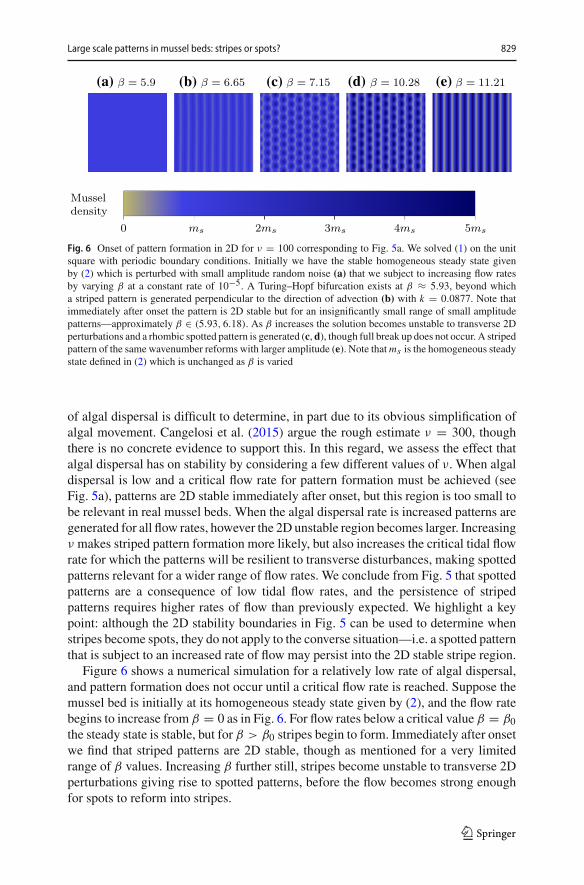
Fig. 6 Onset of pattern formation in 2D for ν = 100 corresponding to Fig. 5a. We solved (1) on the unitsquare with periodic boundary conditions. Initially we have the stable homogeneous steady state givenby (2) which is perturbed with small amplitude random noise (a) that we subject to increasing flow ratesby varying β at a constant rate of 10−5. A Turing–Hopf bifurcation exists at β ≈ 5.93, beyond whicha striped pattern is generated perpendicular to the direction of advection (b) with k = 0.0877. Note thatimmediately after onset the pattern is 2D stable but for an insignificantly small range of small amplitudepatterns—approximately β ∈ (5.93, 6.18). As β increases the solution becomes unstable to transverse 2Dperturbations and a rhombic spotted pattern is generated (c, d), though full break up does not occur. A stripedpattern of the same wavenumber reforms with larger amplitude (e). Note thatms is the homogeneous steadystate defined in (2) which is unchanged as β is varied

of algal dispersal is difficult to determine, in part due to its obvious simplification ofalgal movement. Cangelosi et al. (2015) argue the rough estimate ν = 300, thoughthere is no concrete evidence to support this. In this regard, we assess the effect thatalgal dispersal has on stability by considering a few different values of ν. When algaldispersal is low and a critical flow rate for pattern formation must be achieved (seeFig. 5a), patterns are 2D stable immediately after onset, but this region is too small tobe relevant in real mussel beds. When the algal dispersal rate is increased patterns aregenerated for all flow rates, however the 2D unstable region becomes larger. Increasingν makes striped pattern formation more likely, but also increases the critical tidal flowrate for which the patterns will be resilient to transverse disturbances, making spottedpatterns relevant for a wider range of flow rates. We conclude from Fig. 5 that spottedpatterns are a consequence of low tidal flow rates, and the persistence of stripedpatterns requires higher rates of flow than previously expected. We highlight a keypoint: although the 2D stability boundaries in Fig. 5 can be used to determine whenstripes become spots, they do not apply to the converse situation—i.e. a spotted patternthat is subject to an increased rate of flow may persist into the 2D stable stripe region.

Figure 6 shows a numerical simulation for a relatively low rate of algal dispersal,and pattern formation does not occur until a critical flow rate is reached. Suppose themussel bed is initially at its homogeneous steady state given by (2), and the flow ratebegins to increase from β = 0 as in Fig. 6. For flow rates below a critical value β = β0the steady state is stable, but for β > β0 stripes begin to form. Immediately after onsetwe find that striped patterns are 2D stable, though as mentioned for a very limitedrange of β values. Increasing β further still, stripes become unstable to transverse 2Dperturbations giving rise to spotted patterns, before the flow becomes strong enoughfor spots to reform into stripes.

123

830 J. J. R. Bennett, J. A. Sherratt

We investigated history dependence in mussel beds by using Fig. 5b to informour numerical simulations. Figure 7 shows the results of a simulation in which weslowly oscillated β between maximum and minimum flow rates at a constant rate,which reveals that a number of distinct striped patterns can exist for the same β. Thishysteresis effect is novel due to the fact that transitions are purely a result of transverseinstabilities and are consequently unreported in the literature. If one considered a 1Dtreatment of the problem resulting in the Eckhaus curve alone, onewould conclude thatthe transformation from one striped pattern to another would be a consequence of highflow rates. In contrast, our results provide a more relevant destabilisation mechanismwhen considering the transition between flood and ebb currents during a period oftidal oscillation. Figure 7 also demonstrates that spotted patterns themselves are notnecessarily stable; the spotted pattern in Fig. 7b breaks up, and a new spotted patternemerges in Fig. 7e.

5 Ecological implications and discussion

We have analysed an extended reduced losses model (1) for striped mussel beds thatwas originally posited in two space dimensions (van de Koppel et al. 2005). Nonethe-less, much of the mathematical analysis has focused on the one dimensional case;assuming results can be applied trivially in 2D. The one dimensional solutions areperiodic travelling waves which we extend in two space dimensions as stripe patterns,and analyse using numerical continuation techniques and simulation. Specifically wehave examined how the tidal flow rate affects the resilience of stripes, and we sum-marise the ecological implications as follows.

(i) Our main result is that large scale spotted patterns in mussel beds are a con-sequence of low tidal flow rates. Once a striped pattern has formed, a criticalminimum flow rate must be attained for ecological resilience, otherwise, thestriped pattern is an effective transitional phase in the formation of spotted pat-terns. An ecologist interested in determining resilient striped patterns should notethat β must be stronger than previously thought in this regard. If not, stripes willbreak up and a patchy appearance of the mussel bed may be observed in practice,as seen in Fig. 1. The authors in Siero et al. (2015) determined that striped vegeta-tion patterns in semi-deserts were more resilient on steeper slopes (an equivalentadvection coefficient to β is used to increase the flow rate of water down theslope); in this regard our results are in correspondence.

(ii) A higher rate of algal dispersal in the lower water layer permits the generation ofperiodic stripe patterns at lower flow rates, though additionally it encourages theirbreak up. Although the model we consider incorporates a simple approximationof true algal movement, we can still hypothesise what physical attributes of thesystem might influence ν. The random movement of algae is determined bycomplex mixing processes in the ocean caused by turbulence—primarily on themillimetre scale. Physical properties of the ecosystem that might influence theseprocesses in intertidal regions include: temperature, roughness of the seabed andwave action (Dower et al. 1997).

123

Large scale patterns in mussel beds: stripes or spots? 831

(a)

(c)

(d)

(e)

(f)(g)

(h)

(i)

(j)

(k)

(l)(m)

(n)

(o)

(p)

(b)

Fig. 7 2D hysteresis effects in mussel beds caused by changing tidal currents for ν = 300. We solved (1)on the unit square with periodic boundary conditions. Panels are snapshots of a single numerical simulationof (1), where β varies at a constant rate of 10−4 back and forth between β = ± 40. The relevant stabilitydiagram can be seen in Fig. 5b. Initially, we have a pattern with wavenumber k = 0.04 repeated fivefold(a). As the flow weakens, a spotted pattern emerges (b), breaks up (c), (d) and forms a new regular spottedpattern (e). As the direction of flow changes and strengthens, a striped pattern begins to reform with defects(f) that subsequently disappear leaving a pattern with k = 0.064 (g). As β is varied from −40 to 40 wesee spots (h) that become distorted into droplet shapes (i) and destabilise (j), (k) into a different spottedpattern (l). This pattern reforms into a striped pattern with k = 0.088 (m). Repeating the process using thesolution in (m) as a starting point generates spotted patterns like those in (n), (o), but the reformed stripedpattern (p) is identical to that in (m). Note that in the absence of history dependence one would expect thesame patterns for ±β due to symmetry in (1). Therefore, the red boxed panels demonstrate three distinctstriped patterns for, essentially, the same flow rate

123

832 J. J. R. Bennett, J. A. Sherratt

(iii) We have identified a new type of hysteresis affect in mussel beds that is a resultof small disturbances perpendicular to the direction of tidal flow. Building onprevious work (Sherratt 2013b), our consideration of transverse 2D perturbationsof stripes has revealed new destabilisation mechanisms which cause their breakup. With guidance from the stability map in Fig. 5 we simulated (1) numericallyfor slowly varying β in two space dimensions and find that transitions betweendistinct striped patterns occur as a consequence of the 2D instability. Each stripedpattern is dependent upon the previous state of the system.

The factors mentioned in (ii) that influence the dispersal of algae occur concurrentlyto generate eddies that affect the mixing of algae in a complicated way, the variationof which is crudely reflected in (1) with a change in algal dispersal rate. Due to theobvious model simplification ν is very difficult to estimate, therefore we performedour calculations for a range of values. An interesting direction for further work in thisregard would be to incorporate a more realistic model for the random movement ofalgae, not only in the x and y directions, but also between water layers. Experimentalwork could also aid in the determination of a more informed choice of ν that couldbe used in our calculations. Nevertheless, an extension of the original reduced lossesmodel to include a simplistic random movement term for algae is a more accuraterepresentation of the real world problem, and the consideration of a range of dispersalrates leads us to the conclusion set out in (ii).

The most changeable parameter in (1) is the tidal flow rate, though our analysis hasfocused on the casewhereβ is constant;making our resultsmost relevantwhenβ variesslowly. In reality, the flow rate in intertidal regions oscillates much faster and in a moresinusoidal fashion. Furthermore, a unidirectional flow causes a constant collectivepattern migration in the opposite direction, though there is no evidence to support this.An oscillatory, bidirectional flow ensures that no net migration occurs (Sherratt 2016).Simulations of (1) for a sinusoidal flow rate with maximum amplitude βmax revealsthat stripes may withstand brief intervals of low flow rate. This is dependent on βmax

which, assuming a constant period of oscillation, affects the rate of change of β andthe duration that stripes are subject to the low, destabilising flow rates. Figure 8 showshow βmax affects the long term evolution of stripes when subject to tidal oscillation,and demonstrates how Fig. 5 can be used to roughly gauge the outcome. Note thatapart from β this simulation is identical to that in Fig. 7 and we find that the samewavelength pattern is generated in Fig. 8a as seen in Fig. 7l. For more rigorous results,further work could focus on performing our analysis on (1) with β = β(t). Despitethis shortcoming in our analysis, we believe that (iii) will still be significant in realmussel beds because of slower tidal variations throughout the year. Of course, thereis a regular oscillation of the tidal flow rate during a day, but there are also biweeklyspring and neap tides known for their more extreme tide highs and lows that result inlarger and smaller βmax respectively Lalander et al. (2013); to an extent that dependson the geographical context, for instance basin geometry. Additionally, the relativeposition of the Earth and Moon in their collective elliptic orbit of the Sun gives rise toboth abnormally strong perigean and weak apogean currents that occur three or fourtimes annually (Cartwright 1999). This means that a striped pattern that is resilient toan oscillatory flowwith a particular βmax may be susceptible to break up later on in the

123

Large scale patterns in mussel beds: stripes or spots? 833

(a) (b) (c)

Fig. 8 The effects of oscillating tidal flow are shown through simulation of (1) with β = βmax cos(2π t/T )

for three different values of βmax . Parameters and domain size are identical to that in Fig. 8 with theexception of β, and we use Fig. 5b to inform our choices of βmax . We assume a semi-diurnal tide wheretwo tidal oscillations occur per day, which corresponds to the nondimensionalised time period: T = 2000.Panels are the solutions after 100 tide oscillations (50days) with the addition of random noise every fewtime steps. In all cases a pattern with wavenumber k = 0.088 (identical to that observed in Fig. 7m) emergesquickly. After this: (a) stripes persist despite short intervals of low flow rate, (b) stripes break up to form aspotted pattern which maintains its structure during subsequent oscillations, (c) stripes break up to form aspotted pattern with defects that persist. We solved (1) on the unit square with periodic boundary conditions

year because of a change in βmax . Onemight therefore expect to see a larger proportionof striped mussel beds around the time of a perigean spring tide, and spotted/patchymussel beds around the time of an apogean neap tide. This slow variation in βmax

presents the opportunity for break up and reformation of stripes and the possibility ofobserving the history dependence that we have reported.

In general, testing theoretical predictions aboutmussel beds is certainlymore plausi-ble than formany other ecological systems, e.g. spotted patterns in coral reefs (de Paoliet al. 2017), rows of trees in the ribbon forest (Bekker et al. 2009), banded vegetationin semi-arid desert regions (Klausmeier 1999). This is because pattern generation inyoung mussel beds is relatively fast and small-scale in comparison with the previousexamples. Mussel patterns actually occur on multiple spatial scales (Liu et al. 2014)and previous experiments on small-scale mussel patterns have been possible under labconditions (Van de Koppel et al. 2008). Though harder to implement at the ecosys-tem scale, recent work (de Paoli et al. 2017) has included the seeding of mussel bedsinto various initial formations of large and small scale patterns in order to observehow mussel numbers are affected over time—this enabled the authors to validate thetheoretical prediction that self–organisation increases the resistance of mussel bedsto disturbances. We believe a similar field experiment could be implemented to test(i)—the key feature of this would be to control and measure maximum flow rate. Wepoint out that spotted patterns will be unlikely to form at very low flow rates since thereplenishment of algae would be minimal in reality, leading to the breakdown of themodel and, hence, of our predictions.

Acknowledgements We would like to thank Johan van de Koppel for kindly providing the photograph inFig. 1.

123

834 J. J. R. Bennett, J. A. Sherratt

Open Access This article is distributed under the terms of the Creative Commons Attribution 4.0 Interna-tional License (http://creativecommons.org/licenses/by/4.0/), which permits unrestricted use, distribution,and reproduction in any medium, provided you give appropriate credit to the original author(s) and thesource, provide a link to the Creative Commons license, and indicate if changes were made.

References

Bekker MF, Clark JT, Jackson M (2009) Landscape metrics indicate differences in patterns and dominantcontrols of ribbon forests in the Rocky Mountains, USA. Appl Veg Sci 12(2):237–249

Cangelosi RA, Wollkind DJ, Kealy-Dichone BJ, Chaiya I (2015) Nonlinear stability analyses of turingpatterns for a mussel–algae model. J Math Biol 70(6):1249–1294

Capelle JJ,Wijsman JW, Schellekens T, van StralenMR,Herman PM, SmaalAC (2014) Spatial organisationand biomass development after relaying of mussel seed. J Sea Res 85:395–403

Cartwright DE (1999) Tides: a scientific history. Cambridge University Press, CambridgeChristensenHT, Dolmer P, Hansen BW,HolmerM, Kristensen LD, Poulsen LK, Stenberg C, Albertsen CM,

Støttrup JG (2015) Aggregation and attachment responses of blue mussels, Mytilus edulis—impactof substrate composition, time scale and source of mussel seed. Aquaculture 435:245–251

Cox SM, Matthews PC (2002) Exponential time differencing for stiff systems. J Comput Phys 176(2):430–455

Dame R, Dankers N, Prins T, Jongsma H, Smaal A (1991) The influence of mussel beds on nutrients in theWestern Wadden Sea and Eastern Scheldt estuaries. Estuaries 14(2):130–138

DeconinckB,Kutz JN (2006)Computing spectra of linear operators using the Floquet–Fourier–Hillmethod.J Comput Phys 219(1):296–321

de Paoli H, van der Heide T, van den Berg A, Silliman BR, Herman PM, van de Koppel J (2017) Behav-ioral self-organization underlies the resilience of a coastal ecosystem. In: Proceedings of the nationalacademy of sciences, p 201619203

Dobretsov SV (1999) Effects of macroalgae and biofilm on settlement of blue mussel (Mytilus edulis L.)larvae. Biofouling 14(2):153–165

Doedel EJ, Fairgrieve TF, Sandstede B, Champneys AR, Kuznetsov YA,WangX (2007) Auto-07p: continu-ation and bifurcation software for ordinary differential equations. http://citeseerx.ist.psu.edu/viewdoc/summary?doi=10.1.1.423.2590

Dolmer P (2000) Algal concentration profiles above mussel beds. J Sea Res 43(2):113–119Dower JF, Miller TJ, Leggett WC (1997) The role of microscale turbulence in the feeding ecology of larval

fish. Adv Mar Biol 31:169–220Fiedler B (2002) Handbook of dynamical systems, vol 2. Gulf Professional Publishing, HoustonGascoigne JC, Beadman HA, Saurel C, Kaiser MJ (2005) Density dependence, spatial scale and patterning

in sessile biota. Oecologia 145(3):371–381Ghazaryan A, Manukian V (2015) Coherent structures in a population model for mussel–algae interaction.

SIAM J Appl Dyn Syst 14(2):893–913Guiñez R, Castilla JC (1999) A tridimensional self-thinning model for multilayered intertidal mussels. Am

Nat 154(3):341–357Holzer M, Popovic N (2017) Wavetrain solutions of a reaction–diffusion–advection model of mussel–algae

interaction. SIAM J Appl Dyn Syst 16(1):431–478Hughes R, Griffiths C (1988) Self-thinning in barnacles and mussels: the geometry of packing. Am Nat

132(4):484–491Klausmeier CA (1999) Regular and irregular patterns in semiarid vegetation. Science 284(5421):1826–1828Lalander E, Thomassen P, Leijon M (2013) Evaluation of a model for predicting the tidal velocity in Fjord

entrances. Energies 6(4):2031–2051Liu QX, Weerman EJ, Herman PM, Olff H, van de Koppel J (2012) Alternative mechanisms alter the

emergent properties of self-organization in mussel beds. In: Proceedings of the royal society, TheRoyal Society, London, p rspb20120157

LiuQX,Herman PM,MooijWM,Huisman J, SchefferM,Olff H, VanDeKoppel J (2014) Pattern formationat multiple spatial scales drives the resilience of mussel bed ecosystems. Nat Commu 5:ncomms6234

Newell RI (1989) Species profiles: life histories and environmental requirements of coastal fishes andinvertebrates (north andmid-atlantic): blue mussel. Tech. rep., Army EngineerWaterways Experiment

123

Large scale patterns in mussel beds: stripes or spots? 835

Station, Vicksburg, MS (USA); National Wetlands Research Center, Slidell, LA (USA); MarylandUniv., Cambridge, MD (USA). Horn Point Environmental Labs

Øie G, Reitan KI, Vadstein O, Reinertsen H (2002) Effect of nutrient supply on growth of blue mussels(mytilus edulis) in a landlocked bay. In: Vadstein O, Olsen Y (eds) Sustainable increase of marineharvesting: fundamental mechanisms and new concepts. Springer, Berlin, pp 99–109

Okamura B (1986) Group living and the effects of spatial position in aggregations of Mytilus edulis.Oecologia 69(3):341–347

Rademacher J, Sandstede B, Scheel A (2007) Computing absolute and essential spectra using continuation.Physica D 229:166–183

Sherratt JA (2012) Numerical continuation methods for studying periodic travelling wave (wavetrain) solu-tions of partial differential equations. Appl Math Comput 218(9):4684–4694

Sherratt JA (2013a) Generation of periodic travelling waves in cyclic populations by hostile boundaries.Proc R Soc Lond Ser A 469:20120756. https://doi.org/10.1098/rspa.2012.0756

Sherratt JA (2013b) History-dependent patterns of whole ecosystems. Ecol Complex 14:8–20Sherratt JA (2016) Invasion generates periodic traveling waves (wavetrains) in predator-prey models with

nonlocal dispersal. SIAM J Appl Math 76:293–313Sherratt JA, Mackenzie JJ (2016) How does tidal flow affect pattern formation in mussel beds? J Theor Biol

406:83–92Siero E, Doelman A, EppingaMB, Rademacher JDM, RietkirkM, Siteur K (2015) Striped pattern selection

by advective reaction-diffusion systems: resilience of banded vegetation on slopes. Chaos 25:036411.https://doi.org/10.1063/1.4914450

Tyler-Walters H (2008) Mytilus edulis. Common mussel. Marine life information network: biology andsensitivity key information sub-programme. Plymouth Marine Biological Association of the UnitedKingdom

van de Koppel J, Rietkerk M, Dankers N, Herman PM (2005) Scale-dependent feedback and regular spatialpatterns in young mussel beds. Am Nat 165(3):E66–E77

Van de Koppel J, Gascoigne JC, Theraulaz G, Rietkerk M, Mooij WM, Herman PM (2008) Experimentalevidence for spatial self-organization and its emergent effects in mussel bed ecosystems. Science322(5902):739–742

Wang RH, Liu QX, Sun GQ, Jin Z, van de Koppel J (2009) Nonlinear dynamic and pattern bifurcations ina model for spatial patterns in young mussel beds. J R Soc Interface 6(37):705–718

Affiliations

Jamie J. R. Bennett1 · Jonathan A. Sherratt1

Jonathan A. Sherrattj.a.sherratt@hw.ac.uk

1 Department of Mathematics and Maxwell Institute for Mathematical Sciences, Heriot-WattUniversity, Edinburgh EH14 4AS, UK

123