Modelling of Wet Gas flow in Venturi Meters to Predict the

34th International North Sea Flow Measurement Workshop 25-28 October 2016

1

Modelling of Wet Gas flow in Venturi Meters to Predict the Differential Pressure

H.R.E. van Maanen, Hint B.V. H. de Leeuw, Shell Global Solutions B.V.

1 INTRODUCTION Fossil fuels will remain to provide a large fraction of the world’s energy needs in the decades to come. As natural gas is a relatively clean fuel and because of its abundance, it is expected to be a major contributor. However, virtually all gas-wells produce not only gas, but also liquids, both hydrocarbon condensates as well as water. The latter consists of condensed water and often also formation water. Such flows of gas and liquids are usually referred to wet-gas. In this paper, we will use the term wet-gas for such flows where the Lockhart-Martinelli (LM) parameter is below 0.35 and the flow is not slugging or unstable (e.g. churn flow). Flow rate measurement of wet-gas streams with a dedicated multi-phase/wet-gas flow meter would be beneficial as this is simpler and cheaper than the use of test-separators. We think the performance of such flow meters in general could improve significantly, but it would require a much better understanding of the physics governing the measurement process than is currently available in the public domain. This paper is intended to make a start by disclosing our models for horizontal and vertical Venturis. We hope this will inspire others to come forward with further contributions bringing our collective understanding to a higher level. 2 THE BASIC EQUATIONS Differential pressure flow meters are based on the Bernoulli equation, which states that specific kinetic energy and pressure (specific static energy) are interchangeable:

Cvp =+ 2

21 ρ

(1)

Differential pressure flow meters are designed in such a way that the velocity of the fluid is changed, leading to a change in pressure. The differential pressure is a measure for the flow rate:

ρβ

βε pACQ DD

∆

−= 2

1 4

2

(2)

The actual gas volume fraction is defined as:

liquidgas

gasa QQ

QGVF

+=

(3)

The superficial velocities are defined as:

D

lglsg A

Qv ,

, = (4)


2

The gas Froude number is defined as:

gD

vFr

gl

sgg )(

2

ρρρ−

= (5)

The liquid Froude number is defined as:

gD

vFr

gl

sll )(

2

ρρρ

−=

(6)

With the Lockart-Martinelli parameter defined as:

l

g

g

l

g

l

g

l

g

l

sg

sl

g

l

w

w

Q

Q

v

v

Fr

FrLM

ρρ

ρρ

ρρ ====

(7)

The overreading of a differential pressure flow meter in wet-gas is defined as:

go

tp

p

pgOverreadin

∆∆

= (8)

It is possible to derive the overreading analytically under the assumption that the flow is either fully stratified or when it is a homogeneous mist flow in which the liquid is fully dispersed as small droplets. The results are given below without derivation. These can be found elsewhere. The overreading in a stratified flow is:

LMgOverreadin += 1 (9)

The correlation of Murdock[1] is based on this equation, but a constant was added to fit his experimental data better. The overreading of a mist flow is:

25.05.0 ])()[(1 LMLMgOverreading

l

l

g +⋅++=ρρ

ρρ

(10)

Note that the overreading of the stratified flow can be rewritten as:

2002 ])()[(1211 LMLMLMLMLMgOverreading

l

l

g +⋅++=+⋅+=+=ρρ

ρρ

(11)

The overreading has been described in several correlations and we will discuss two of these here. The first is the correlation of Chisholm[2]. His correlation reads:

225.025.0 ])()[(1 LMLMgOverreading

l

l

g +⋅++=ρρ

ρρ

(12)

As Chisholm did the experiments, on which his correlation is based, at relatively low pressures and with air-water, it is likely that his flow regime was stratified entrained. So his value of 0.25 in the above equation, halfway between zero and 0.5, seems not unrealistic. De Leeuw[3], having gathered a large set of experimental data up to higher pressures and gas Froude numbers and subsequently building on the above equations, modified it by introducing a parameter “n”:


3

2])()[(1 LMLMgOverreadin n

g

ln

l

g +⋅++=ρρ

ρρ

(13)

In which n is taken as a function of the gas Froude number:

41.0=n 5.15.0 << gFr

)1(606.0 746.0 gFren −−⋅= 5.1>gFr

Both the correlations of Chisholm and De Leeuw predict the overreading in the limiting cases of LM ↓ 0 and the dense phase ρg ↑ ρl correctly. An interesting

aspect of the correlation of De Leeuw is that it predicts an overreading above the overreading for the homogeneous mist flow which, at first sight, seems to be the upper limit for the overreading. We will park this question for the moment and come back to this issue later. We will first discuss the limitations of correlations. 3 THE LIMITATIONS OF CORRELATIONS Correlations are basically mathematical curve fits through experimental data points. Some correlations, like those of Chisholm and De Leeuw, use a basic equation for the phenomenon they want to curve-fit, whereas others, like the one of Steven[4], use equations which are not necessarily related to a basic equation. Although some speak of “models” in this case, this is incorrect as it is not based on physics. Strictly speaking, correlations are only valid within the range of the experimental data on which they are based and validated. Therefore it is possible that correlations do not predict limiting cases correctly when these lay outside the range of the experimental data. As stated before, the correlations of Chisholm and De Leeuw predict the limiting cases correctly and a requirement for correlations could be that these include the limiting cases for which the behaviour is known. However, a large problem with correlations is that these include a number of parameters to enable the use of the correlations with fluids with different physical properties. The selection of the parameters is educated guesswork and is often enforced by the limitation of the fluid properties which could be used during the experiments on which the correlation is based. However, there is no guarantee that all essential parameters are included in the correlation. In general, it is impossible to include all important properties in the experiments: the number of required data-points will simply become too large. So unless a better understanding of the physics, which govern the measurement process, is obtained, no guarantee can be given that correlations give correct and accurate predictions when the physical properties of the fluids used in the application are different from those in the experiments (and they always will). As a consequence, a narrow fit in a tested range does not imply any accuracy in other ranges and or other fluids. Only when there is a good understanding of the governing physics, the essential physical properties can be revealed and it will become possible to predict the overreading in application with different conditions, e.g. pipe diameters, different β-ratios and different fluids. Also, applications outside the range of the experimental data become more trustworthy, thereby greatly extending the possibilities to apply wet-gas flow rate measurement in practice.


4

To avoid the use of correlations this paper presents the models developed for a wet gas flow through a horizontal Venturi and through a vertical upward Venturi. Both models will be described in the sections below. 4 THE EXTENSION OF THE BERNOULLI EQUATION The Bernoulli equation is only valid for systems with no energy loss. When energy losses do occur, correction term(s) need to be added. This is illustrated by e.g. the orifice meter. It is well known that the discharge coefficient of an orifice is roughly 0.6, which can be interpreted in the following way:

dBO ppp ∆+∆=∆ (14)

It can be remarked that (eq. 2)

ODB pCp ∆=∆ 2

(15)

Reworking the two equations above yields:

ODd

dODO

pCp

ppCp

∆⋅−=∆

∆+∆=∆

)1( 2

2

(16)

So with a discharge coefficient of 0.6, the contribution of the ideal Bernoulli equation to the differential pressure is 36% and 64% is generated by dissipation. This explains why the pressure recovery of an orifice is only minor. A Venturi with a discharge coefficient of 0.995 thus has only 1% of the differential pressure generated by dissipation, so it is expected that its pressure recovery is significantly higher than that of an orifice. However, in the divergent section, significant turbulence is generated, leading to additional dissipation. Which is why the Venturi still has a noticeable total pressure loss, which depends on its construction. Therefore it is clear that, in order to describe the differential pressure of a Venturi in a wet-gas flow, a dissipation term needs to be added to the Bernoulli equation. Implicitly, the rising of the “n” value above 0.5 in the correlation of De Leeuw is the inclusion of such a dissipation term. It does, however, not describe the size and the cause(s) of the dissipation. The given that the “n” value can become larger than 0.5 and knowing that the total pressure loss ratio of a Venturi is in a wet-gas flow significantly higher than in a single phase flow, reveal that already energy is dissipated upstream of the throat pressure tap. This will have to be included in the model. It is to be expected that the dissipation mechanisms in a horizontal and a vertical upward Venturi are different. Because of the size limitation, it is not possible to include all the details and all the required equations into this paper. The crucial steps, however, will be described and discussed. For more details, the authors can be approached. As we do not have the possibilities to develop these models further on our own, we welcome any person or institution to bring this work further. We can provide the current state of the development and may provide data-sets from tests under realistic conditions. 5 MODELLING OF HORIZONTAL FLOW IN VENTURIS The modelling of the differential pressure inlet – throat is based on an extension of the Bernoulli equation and will include the contributions by the gas, the


5

dispersed liquid(s), dissipation terms and some smaller contributors. This approach leads to the following equation:

[ ] p + N + N + N + Av + Av + Av

2

1 = N dissplstlflf

2

llgd2

lgg2

gt ρρρ (17)

Note that for the calculation of vg, Ag, vd, Alg, vlf and Alf the local hold-up is required. Its calculation has been done by the authors, but this not included in this paper to limit its length. The challenge is to determine the different contributors to this equation under realistic conditions. To indentify these, several parameters need to be known. Therefore, we will give a description of the wet-gas flow upstream and moving into the Venturi up to the throat pressure tap. Upstream of the Venturi, a partly entrained, partly stratified-wavy flow regime is maintained. The energy of the moving fluids upstream of the Venturi is dependent on the entrained fraction. Correlations for the entrained fraction can be found in literature[7], we used the Shell Vassiliadou relationship[5]:

factor + 1

factor E = E Mf

(18)

in which:

w

w - w 0, = El

cl,lM max

(19)

and factor is:

f v ) ( g ) - (

1.27 = factor sgsg51.5

gllgl

g ρρσρρρ

η

(20)

and fsg is the friction factor, smooth pipe, turbulent flow, based on superficial gas velocity:

Re

0.046 = f

sg0.2sg

(21)

and Resg is:

η

ρ

g

gsgsg

D v = Re

(22)

Once the entrained fraction is determined, the energy of the moving fluids can be found using the quasi Lockhart-Martinelli parameter, derived in Appendix 1:

LM

LM + 1 v ) E - (1

2

1 + )LM + (1 v

2

1 = E

q

qsl

22flqmixs,

2mix ρρ

(23)

When the fluids move into the convergent section of the Venturi, the gas will start to accelerate. Due to the inertia of the droplets, these will lag the gas. This has two major consequences: the first is dissipation because of an increase in the velocity difference between the gas and the droplet, the second is an increase of the drag force on the droplet. When the drag force exceeds the surface tension,


6

the droplet is no longer able to withstand the increasing force and it will break up into smaller droplets. In the calculation, this is approximated by the split of the droplet into two with identical sizes. This phenomenon also explains why the Venturi acts like a nozzle and the average droplet diameter in the throat is smaller than upstream of the Venturi. A major consequence of this description is that the surface tension is an important parameter, which now will be included. The accelerating gas also creates an increasing shear on the gas-liquid interface, which will enhance the entrainment of droplets itself. The Vassiliadou relationship yields unrealistically high values for the entrained fraction, certainly at higher liquid loadings, as it is impossible to entrain so much liquid in the short time that the fluids stay in the convergent section of the Venturi. However, no reference which describes these phenomena has been found the in the open literature, therefore, a novel correlation has been introduced, based on the SINTEF and CEESI data-sets:

ρρ

l

g

0.29

0.285 = er (24)

Note that the entrainment rate has the dimension of m/s, in order to calculate the actual volumetric entrainment, the value needs to be multiplied by the surface area from which the entrainment takes place. The entrainment rate thus shows to be a shallow function of the ratio of the gas and liquid densities. Although these assumptions are only an approximation of reality, we think that this is the best approach available at the moment, although we realise that future work might bring better relationships. However, the complete model described here has been tested with experimental data from K-lab with a different Venturi, a different β-ratio and different fluids and it performed very well. 5.1 The Dissipation of the Gas Flow Around the Droplets The normalised dissipation energy Ndiss has two contributing components:

N + N = N srdgdiss (25)

The above described mechanisms enables the calculation of the contribution to the differential pressure by the Bernoulli effect of the gas, the entrained liquid and the liquid in the film and the dissipation due to the gas flow around the droplets. However, the contributions caused by the dissipation due to the interfacial roughness, the increase in potential energy of the stratified liquid (the throat is at an elevated level) and the energy stored in the surface tension (in the throat more and smaller droplets are present) still need to be included. The drag force on the droplet is equal to:

v

2

1 d

4

1 C = F 2

rg2

wd ρπ (26)

The drag coefficient is found from:

0.44 +

Re

24 = C w

(27)


7

in which Re is:

η

ρ

g

gr d v = Re

(28)

This is a well-known and often used correlation for spherical bodies and has been used here[6]. 5.2 Other Contributors to the Differential Pressure It is assumed that the entrainment and deposition of the droplets upstream of the Venturi are in equilibrium and that at the entrance of the convergent section of the Venturi the droplets move with the gas velocity. If they would not, the gas would exert a force on the droplet until they did. This assumption does not take into account that the droplets have a limited "lifetime", i.e. are created with a velocity below the average gas velocity and are re-deposited in the liquid film after a certain time (which is probably random). However, the entrained fractions in the pipe, upstream of the Venturi, are relatively low and therefore the error in the determination of the kinetic energy of the entrained liquid will be small. On top of this, the kinetic energy of the moving fluids upstream of the Venturi is only a small term in the energy balance and hence has a small effect, except for a relatively large β-ratio (say > 0.7). The droplets which are entrained in the convergent section of the Venturi are given an initial velocity equal to the velocity of droplets already entrained. Although this is not completely realistic, it is a reasonable assumption and it simplifies the calculations. Note that the surface of the liquid layer, from where the droplets are torn from the liquid film, has a velocity which is roughly twice the average velocity of the liquid film due to the linear velocity profile in the liquid film. On top of that, the gas velocity close to the gas-liquid interface is lower than the average gas velocity, due to the friction at the gas-liquid interface. Thus, the velocity difference between the newly entrained droplets and the gas surrounding these, should therefore be in the same order of magnitude as that of the already entrained droplets. This velocity difference is more important than the absolute velocity and in case it would be significantly larger, it would result in break-up of the droplets. The liquid film in the convergent section and the throat gives rise to a rough surface, which causes viscous dissipation in a similar way as in normal pipe flow. The surface roughness is taken as 0.085 m; m = liquid film thickness; the film is assumed to have a constant thickness across the circumference. However, the contribution to the dissipation is small but increases with decreasing gas density. The reason is that at the lower gas densities the hold-up is higher and the entrained fraction is lower. Both result in an increased surface roughness and thus friction factor. The surface tension of the droplets represents an amount of energy, which increases as the total surface of the droplets increases when the fluids move through the Venturi up to the throat. The calculation of this contribution can be found in Appendix 3. When the liquid is lifted from the lower half of the pipe into the throat of the Venturi, the potential energy of the liquid increases. This energy is delivered by the flow, thus increasing the pressure change. The liquid will -in the majority of the cases- be partly stratified. The potential energy of the liquid which stays in


8

the liquid layer at the bottom will increase due to the higher level of the throat. The potential energy of the liquid, entrained into the gas, increases even more as it is lifted from the liquid layer. This results in relatively more significant contributions at the low gas Froude numbers. At the lowest gas Froude number, the liquid is damming up against the throat, which means that the raise in potential energy is already partly completed by the time the liquid reaches the upstream pressure tap as is illustrated in fig. 1.

Figure 1: The damming of the liquid up against the throat. Note the compression

of the horizontal scale to elucidate the effect. Note that due to this liquid build-up, the gas velocity at the upstream pressure tap is higher than without it. So far, this phenomenon is not included in the model and could give rise to an over-prediction of the differential pressure at low gas Froude numbers. 6 MODELLING OF UPWARD FLOW IN VENTURIS In a vertical upward wet-gas flow, the gas is the “continuous phase”. The liquids are partly dispersed as droplets in the gas, partly moving as a film at the wall. Due to turbulence in the gas core, droplets will be deposited in the film at the wall and droplets will be torn off the wavy gas-liquid interface. Due to gravity, the liquids will move slower than the gas as the gas has to lift the liquids against the gravitational force. We will refer to this velocity difference as the “slip velocity”. The realization of the inlet-throat differential pressure has a number of different contributors: • The Bernoulli dP caused by the gas • The Bernoulli dP caused by the liquid droplets • The Bernoulli dP caused by the liquid film • The dissipation of the gas flow around the droplets • The dissipation due to viscous forces in the liquid film • The increase in potential energy of the liquid • The energy, stored in the surface tension of the droplets The modeling will require a description to quantify the different contributions. Note that some contributions are irreversible, which means that the total pressure loss (ratio), the outlet-inlet differential pressure, will be larger than in a single-phase system. The modeling will be described below in several separate steps. 6.1 The Dissipation of the Gas Flow Around the Droplets The droplets are lifted against gravity by the friction of the gas flow around them. However, there are some limitations. The first question is the maximum droplet diameter which will occur in such a flow under the given conditions.


9

Basically, there are three forces acting on the droplet: the drag force of the gas flow around the droplet, the gravitational force and the surface tension. With increasing droplet diameter, the gravitational force increases rapidly (with the third power of its diameter), which has to be balanced by the same increase in the drag force. But this force is acting on the surface of the droplet and it is not hard to see that at a given diameter the surface tension is no longer able to maintain the integrity of the droplet: the drag force simply tears it apart. Using this reasoning, we can predict the maximum size of the droplet: it is the diameter at which the surface tension balances the drag force (which balances the gravitational force). The gravitational force, acting on the droplet, consists in itself on two forces: one is the gravitational force, caused by its mass and the Earth’s gravitational acceleration, the second is the hydrostatic force because the droplet is immersed in gas phase. It is not hard to combine these two and the result (net) gravitational force is:

F d gg l g= −

πρ ρ

63 ( )

(29)

The drag force, acting on the droplets is proportional to the cross-sectional area of the droplet, the kinetic energy of the gas phase, relative to the droplet velocity, i.e. the slip velocity and the so-called drag coefficient. In equation;

F C d vd w g r= ( )( )

πρ

4

1

22 2

(30)

We will use the same drag coefficient as in the model for the horizontal Venturi. The surface tension creates a pressure differential with the surrounding gas, which is described for a stationary (relative to the gas) spherical droplet given by the Young-Laplace equation:

∆ p

rd

= σ ( )2

(31)

The force can be found by multiplying the pressure differential by the surface area, but we are not talking about a stationary droplet, but a droplet which is moving through the gas phase. Also, we are looking at a droplet which is at its maximum diameter under such conditions, i.e. at the verge of break-up. Therefore we need to take into account that the surface tension is counteracting the drag force, which acts on the lower half of the droplet and that the droplet, under these conditions, is not spherical anymore, but elongated. Therefore, the Young-Laplace equation cannot be used directly and a different radius has been chosen, related to the lower half of the surface area and the volume related to it to compensate for the above mentioned effects:

r

r

rre

d

dd= =

43

3

22

2

3

ππ

.

. (32)

This radius represents the curvature at the “tip” of the ellipsoid, we will use for the radius at middle of the ellipsoid (where the drag force is the largest and will split the droplet as twice this value. The force subsequently becomes

∆ p r

rr

rr dd

ed

dd. . (

.). . ( ). . . .2

2

22

22

3

22 2

43

2π σ π σ π π σ= = = (33)

Equating this with the drag force yields:


10

C d v dw g r( )( ) . .

πρ π σ

4

1

2

3

22 2 =

(34)

or

C d vw g r( ) .

1

262ρ σ=

(35)

which is the equation used to determine the maximum diameter of the droplet under dynamic conditions. We will also use this equation to determine the locations of break-up of droplets in the accelerating flow in the convergent section of the Venturi, which will be discussed below. The relation between vr and d can be found by balancing the equations for the drag and gravitational forces and solving Cw from these:

C d g d vw g g g r= − − − −( )( ) ( )( )

πρ ρ π ρ

6

423 2 1 2

(36)

from which follows:

C d g vw l g g r= − − −4

31 2( )ρ ρ ρ

(37)

Multiply both sides with Re2:

C d g vv d

w l g g r

r g

g

Re ( )2 1 2

2 2 2

2

4

3= − − −ρ ρ ρ

ρη

(38)

Substituting the correlation for Cw in the above equation yields:

(Re

. ) Re ( )24

0 444

32 3 2+ = − −d gl g g gρ ρ ρ η

(39)

Using this quadratic equation, Re can be solved directly at a given diameter and thus vr, yielding starting values for the determination of the maximum diameter using e.g. the Newton-Raphson technique. A correction is applied for the elongated shape of the droplets. Under the assumptions, described above, the mass of the droplet is twice of that of a spherical droplet with the same radius of curvature at the bottom. The dissipation around the droplet is calculated in the same way as in the model for a horizontal Venturi as described in Appendix 2. This algorithm is also used in the convergent section of the Venturi. The contribution to the differential pressure is found by multiplying the energy dissipation for each (initial drop) with the number of drops per m3. However, two problems arise at this point: • not all the liquid is entrained as droplets as a part is flowing in the liquid film

at the wall, so the “entrained fraction” needs to be determined and • the droplets move slower than the gas, which needs to be corrected for. The first is rather trivial, the second less, but it can be understood by looking at a situation in which the gas velocity is so low that it can not lift the droplets (i.e. vg = vr). In such a case, the dissipation for each droplet would be infinite, as the dissipation will continue, but the droplet will never pass the throat tap.


11

There is a further complication as the gas velocity is higher than the superficial gas velocity. But is also higher than the superficial gas velocity divided by the gas volume fraction (GVF), because that would only be valid if gas and liquid would move with the same velocity. But because the liquid lags the gas, a correction needs to be made by the hold-up or slip between the phases. Note that because of the high GVF in wet-gas flows (>95 %), the corrections are not very large, so we can use some approximations: • we will assume that all liquid is entrained as droplets • we will use the superficial gas velocity to do the initial calculation of the slip

velocity Using these approximations, the gas velocity can be calculated using:

v

v Qv

vQ

Qg

gs g

gs

dl

g

=+.( . )

(40)

If desired, one can use this value as a first estimate for the actual gas velocity and subsequently use this value to get a better estimate for the gas velocity by replacing vgs / vd by vg / vd as this yields a more accurate result. However, even at 95% GVF and a gas velocity only three times the slip velocity, the second iteration is only 0.2% different from the first value, which is a negligible difference as in most other cases the correction will even be smaller. The contribution of the dissipation to the differential pressure inlet-throat of the Venturi thus becomes:

∆ p P E N

v

vd d f d

g

d

= . . .( ) (41)

The number of droplets per cubic meter of gas can be found directly from the liquid volume fraction (LVF) and the droplet diameter:

NQ

Q Q dd

l

l g

=+( ).( )

π6

3

(42)

6.2 The Liquid Film Modeling To model the liquid, flowing in the film at the wall, is the most difficult part of the wet-gas modeling. Therefore, we will first give a qualitative description of the phenomena, which take place and subsequently describe how these can be quantified. There are four forces acting on the liquid, flowing in the film: • the gravitational force • the shear force, caused by the gas flowing along the gas-liquid interface • viscous forces, caused by the velocity gradient in the liquid film, a

consequence of the stationary wall. • Pressure forces due to the Kelvin-Helmholtz phenomenon. The gravitational force will tend to induce a downward flow in the liquid, which is counteracted by the shear of the upward moving gas at the gas-liquid interface. To get a feeling for these forces, let us write down the basic equations under the


12

assumption that the thickness of the liquid layer is very small, compared to the internal pipe diameter. The gravitational force will then be:

F D D L gg lf l= π ρ. . . . .

(43)

The shear force can be calculated using the pressure drop for pipe flow:

∆ p f

L

Dv vg g i= −4

1

22( )( ( ) )ρ

(44)

From this, the wall shear stress can be derived using the balancing of the wall shear stress and the pressure drop:

πρ π τ

44

1

22 2D f

L

Dv v D Lg g i i( )( ( ) ) . . .− =

(45)

from which follows:

τ ρi g g i

fv v= −

22( ) (46)

So the problem boils down to the calculation of the Fanning friction factor f. In literature, the Colebrook correlation[8] is often used. It is an implicit correlation, which, however, gives good results. The Colebrook correlation reads:

12

37

2 5110f f

kD= − +.log (

( )

.

.

Re) (47)

In this case, the waves on the gas-liquid interface act as the surface roughness for the gas flow. We will assume that the amplitude of the waves is 0.75 times the average thickness of the liquid layer, so the peak-to-peak value is 1.5 times the average thickness and we will use this value for the surface roughness k. Basically, the internal diameter should be corrected for the reduction due to the liquid film, which has a double influence on the Reynolds number: both by the internal diameter and the gas velocity. But because the Fanning friction factor is, at higher Reynolds number, virtually independent of the Reynolds number, we can use the “dry” internal diameter and the superficial gas velocity. The Colebrook correlation can be solved by iteration. Usually, within 4 or 5 steps, the result has converged to its final value. This is simpler than using the Newton-Raphson method and about as fast. Using the thus obtained value of the Fanning friction factor, we can calculate the maximum liquid film thickness which can be held up by the interfacial shear stress against gravity. By assuming that vi is 0 (zero) both the interfacial wall shear stress and the gravitational force can be calculated. Using the Newton-Raphson method, the maximum thickness can be calculated. Good starting values are e.g. 0.1, 1 and 5 mm thickness for the liquid film. The shear on the interface, however, can tear off droplets from the liquid film. We will model this as follows: • The wavelength of the waves on the gas-liquid interface is proportional to the

amplitude (and thus of the liquid film thickness, as we assume that the amplitude is 0.75 times the average liquid film thickness, see above) and proportional to the dynamic viscosity of the liquid.


13

• When the shear force exceeds the surface tension at the wave crest, a droplet is torn off, which will thus limit the liquid film thickness.

It is not unrealistic to assume that the waves scale with the liquid film thickness and as the waves induce liquid motion, it is likely that the wavelength will increase with the liquid viscosity. Whether this is proportional is not unrealistic, but unproven. However, as the range of viscosities in wet-gas well flows is not that high, it is likely to be a good starting point. As a starting value, to be refined by validation with experimental values, we will use the viscosity of water at 20oC as reference value. The equation for the wavelength is:

λ πη

η= 2 0 7520

. .( . ),

d lfl

w (48)

The rw is the radius of curvature at the wave crest is:

r

aw =λπ

2

24 (49)

By using the Young-Laplace equation in its two-dimensional form:

∆ pr rw y

= +σ ( )1 1

(50)

and noting that ry, the curvature in the tangential direction, is very high, it can be written as:

∆ pr

a

dw lf

w

l

= = =σπ σλ

σ ηη( )

..( )

,1 4

0 75

2

2

20 2

(51)

When this value exceeds the wall shear stress, droplets are torn off, thus limiting the liquid film thickness. As the wall shear stress also depends on dlf, the use of the Newton-Raphson method to find the maximum liquid film thickness, allowed by the surface tension, is recommended. The third limitation for the thickness of the liquid layer at the wall comes from the velocity gradient in the liquid layer in combination with the liquid viscosity. We will assume that we have a linear velocity gradient in the liquid layer and the shear stress at the wall is given by:

τ η

∂∂w l

zv

r=

.

. (52)

In a steady-state condition, this is equal to the interfacial shear stress and the gravitational force on the liquid. Assuming a linear velocity profile in the liquid film, vi becomes:

v

v

rdi

zlf=

∂∂.

..

(53)

As vi increases with increasing dlf, (vg – vi) decreases. As the interfacial shear stress decreases with decreasing (vg – vi), this puts an upper limit on the liquid film thickness, which can be determined using the Newton-Raphson method. The downward force in the liquid film consists of two components: the gravitational force and the viscous force due to the velocity gradient in the film. If we assume a linear velocity profile in the film, the viscous force is equal to:


14

Fv

dD Lv

i

lfl= . . . .η π

(54)

The gravitational force is equal to:

F D L d gg lf l= π ρ. . . . .

(55)

The total downward force thus becomes:

Fv

dd g D Ldt

i

lfl lf l= +[ . . . ]. . .η ρ π

(56)

Now an interfacial velocity needs to be chosen which balances the downward force and is just not able to tear off droplets from the interface:

τ η ρii

lfl lf l

v

dd g= +. . .

(57)

The criterion for the tearing of droplets from the film is:

τσ η

ηilf

w

ld=

0 7520 2

..( )

,

(58)

Equating both equations to eliminate the interfacial shear stress yields:

v

dd g

di

lfl lf l

lf

w

l

. . ..

.( ),η ρ

σ ηη+ =

0 7520 2

(59)

which is an explicit equation of the liquid film thickness as a function of the interface velocity. From this follows:

0 75 0 752 20 2. . . ( ) . .

,g d vl lf

w

li lρ σ

ηη η= −

(60)

The interface velocity can be calculated using the equation above and the Colebrook correlation.

τ ρi g g i

fv v= −

22( ) (61)

The Fanning friction factor is a function of the liquid film thickness and the liquid viscosity. So combining this equation with the equation for the downward force yields:

v

dd g

fv vi

lfl lf l g g i. . . ( )η ρ ρ+ = −

22

(62)

is an explicit equation for vi with a given dlf. A fourth mechanism is responsible for the limitation of the liquid film thickness, especially at higher velocities. This is caused by the Kelvin-Helmholtz mechanism. An undulation on the liquid film will lead to a pressure undulation because the gas velocity will vary. When this pressure undulation exceeds the surface tension, it will tear off droplets and thus reduce the film thickness. This can be quantified by the equations below. For the derivation of the equations, we will first assume that the waves at the gas-liquid interface are encircling the complete circumference of the pipe. The concept is that the force, generated by the increase of the gas velocity over the wave crests, has to be balanced by the surface tension. If this force exceeds the


15

surface tension, drops will be torn off the surface, reducing the liquid film thickness. The differential pressure, generated by the surface tension, has been derived above:

∆ pd lf

w

l

=σ η

η0 7520 2

..( )

,

(63)

The differential pressure, caused by the Kelvin-Helmholtz effect is equal to:

∆ p v vg g= −1

22 1

22ρ ρmax min (64)

v

Q

Dg

maxmin

= π4

2

(65)

v

Q

Dg

minmax

= π4

2

(66)

in which:

D D d lfmin ,max= − ⋅2

D D d lfmax ,min= − ⋅2

(67)

Using the assumption that the wave amplitude is 0.75 of the average liquid film thickness (see above), the following relations hold:

D D d lfmin .= − ⋅35

D D d lfmax .= − ⋅05

(68)

When we square these diameters we will assume that dlf « D , we will ignore terms of dlf

2 which results in:

D D D d lfmin ( )2 7≈ ⋅ − ⋅

D D D d lfmax ( )2 ≈ ⋅ −

(69)

Knowing that

Q D vg sg= π

42

(70)

we obtain:

vD

D dv

lfsgmax ( )2 2 2

7=

− ⋅ (71)

vD

D dv

lfsgmin ( )2 2 2=

− (72)

Again ignoring the quadratic terms of the small fractions and using the approximation:

1

11

−≈ +δ δ

(73)

when δ « 1, we obtain:


16

∆ p

d

Dvg

lf

sg=⋅

12

212

ρ (74)

If we assume that the wave covers only ¼ of the circumference of the wall, the equation becomes:

∆ p

d

Dvg

lf

sg= 32

2ρ (75)

Equating this to the differential pressure, created by the surface tension leads to:

32

2 20 2

0 75ρ

σ ηηg

lf

sglf

w

l

d

Dv

d=

..( )

,

(76)

Solving dlf from this equation and putting 1.125 ≈ 1 (as there are a number of “guessed” values in this number anyway), we obtain:

dD

vlfg sg

w

l

=⋅⋅

σρ

ηη2

20.( )

,

(77)

The determination of the liquid film thickness using the Kelvin–Helmholtz mechanism limits the liquid film thickness at the higher liquid flow rates and results in more realistic entrained fractions. In this way, a fourth criterion for the determination of the liquid layer is introduced. The criteria so far are: 1. The balance of the gravitational force, the wall shear stress and the gas-liquid

interfacial shear force. 2. The transportation capacity of the liquid film as determined by the first

criterion. 3. The tearing of droplets from the gas-liquid interface due to the shear force. 4. The liquid film thickness as determined by the Kelvin–Helmholtz mechanism. It is obvious that the lowest value of the four limitations on the maximum thickness should be chosen. Once this has been done, the liquid velocity (vi) at the gas-liquid interface can be determined. From this, the volumetric flow rate of the liquid in the film can be calculated under the assumptions of the linear velocity profile in the film and dlf << D, the internal pipe diameter:

Q D d

vlf lf

i= π. . .2 (78)

Note that because the above mentioned assumptions the average velocity in the liquid film is vi / 2. The entrained fraction is:

l

lflf Q

QQE

−=

(79)

Note that the entrained liquid moves as droplets, dispersed in the gas. 6.3 The Prediction of the Differential Pressure of the Venturi Using the above obtained information, the actual gas velocity, the velocity of the droplets, dispersed in the gas and the velocity of the liquid in the film can be calculated and the Bernoulli contributions to the differential pressure can be


17

calculated, taking the break-up of the droplets in the Venturi into account. Similarly, the dissipation contribution can be calculated as described in sec. 3.2 and also the contribution of the surface tension (note that the significant drop in the diameter of the droplets increases the energy, stored in the surface tension). The raise in potential energy can also be calculated, but one should realize that the for the droplets, the difference in density between the gas and the liquid needs to be used whereas for the liquid in the liquid film, the liquid density only should be used, because it is not immersed in the gas. The final contribution comes from the friction of the liquid at the pipe wall because of viscosity. The Bernoulli contributions For the calculations of the Bernoulli contributions of the different phases, several aspects need to be taken into account. These are: 1. The actual velocities of the phases need to be used, both in the pipe as in the

throat of the Venturi. 2. The fraction of the cross sectional area, taken up by the phases need to be

included in the calculation. 3. The contribution of the liquids needs to be separated in the entrained liquid

and the film. Both require the weighted average density of the liquid, which is different for the film and the droplets.

4. It is assumed that the phases do not change while traveling through the Venturi, i.e., no gas comes out of solution from the oil and the entrained fractions remain the same.

Ad 1 As the kinetic energy directly depends on the velocity, this is logical. So the superficial velocities need to be converted to actual velocities. For the gas, this means that the effective diameter of the pipe is reduced, due to the presence of the liquid film and the gas velocity is further increased because of the presence of droplets, which also move slower than the gas. The latter acts as an increase of the liquid volume fraction. Both effects can be described by the following equation:

vQ

D d

v

v vE LVFg

g

p lf

g

g sf=

−+

−π4

21

2( )( . . )

(80)

Note that the entrained fraction in the above equation is the entrained fraction for the total liquid flow rate. The same holds for the liquid volume fraction. The calculation of the liquid film thickness and the slip velocity needs to be done for the pipe and the throat and the resulting velocities need to be used for the calculation of the Bernoulli contribution of the gas, which subsequently needs to be corrected for the fraction of the cross sectional area, taken up by the gas (see Ad 2 below). The slip velocities for the droplets can be calculated using the equations as described in sec. 3.1 and 3.2. Note that the slip velocity in the pipe is influenced by the parameter (currently chosen to be 0.7, see sec. 3.4.2 below) which corrects for the droplet size distribution and that the droplet velocity in the throat still lags the equilibrium velocity. The average velocity of the liquid film is the interface velocity divided by 2. The interface velocity in the throat is significantly different from that in the pipe, but both can be calculated using the theory as described in sec. 3.3.


18

Ad 2 The contribution to the Bernoulli differential pressure needs to be corrected for the fraction of the cross-sectional area, taken up by the fluid. This is logical, because if that would not be done, a few drops of liquid would result in a major increase in the differential pressure, which is not realistic. The following equations can be used:

A A Ag d lf+ + = 1

(81)

Av

vg

sg

g

= (82)

A E LVFv

v vd f

g

g s

=−

. .( ) (83)

Ad

Dlf

lf

p

=4

(84)

The resulting dPB thus becomes:

dP A dP A dP A dPB g Bg d Bd lf Blf= + +

(85)

Ad 3 Because the liquid consists of two immiscible fluids (oil and water), with different entrained fractions, the weighted densities of the liquid in the film at the wall and dispersed as droplets in the gas are different. These can be calculated using:

ρρ ρ

d

o f o o w f w w

o f o w f w

Q E Q E

Q E Q E=

++

. .

. ., ,

, , (86)

ρρ ρ

lf

o f o o w f w w

o f o w f w

Q E Q E

Q E Q E=

− + −− + −

( ) ( )

( ) ( ), ,

, ,

1 1

1 1 (87)

Ad 4 When the fluids move through the Venturi, the velocities and pressure change. Also, the geometry is not “straightforward”, which –in principle- all have an effect on the gas-liquid ratio and entrained fractions. The drop in pressure between the inlet and the throat of the Venturi will lead to gas, coming out of solution from the oil. This process is very hard to describe on the time scales of the fluids moving through the Venturi and therefore, it is recommended that the pressure changes are modest, compared to the absolute pressure (< 2%). In this way, it is expected that the effects remain negligible. In the convergent section of the Venturi, several phenomena will take place. Because of the decrease of the cross-sectional area, droplets will be deposited in the liquid film at the wall, but because of the increase in the gas velocity, droplets will be torn off the liquid film more easily. The entrance of the throat will act as a nozzle, increasing the entrained fraction. This is very hard to model and therefore, because of the countering effects, we will assume that the net-effect is zero. 6.4 Refinement of the Initial Conditions Direct application of the equations, as outlined above, will result in a droplet diameter at the entrance of the Venturi which is at its maximum. This is probably


19

not realistic as due to turbulence, differences will occur. In general, the droplets will show a size distribution with a maximum value as calculated above. But it is very hard to measure the droplet size distribution. Using a droplet size distribution would also complicate the calculations so it is simplified by using a single value of the droplet diameter at the entrance of the Venturi, albeit smaller than the maximum value. A diameter, which is 0.7 times the maximum possible diameter will be used. Fortunately, the calculated dissipation is not strongly dependent on the initial conditions, but it tends to decrease slightly with decreasing diameter at the entrance of the Venturi. It may require some “fine tuning” using experimental data. 6.5 Refinement of the Presence of Three Phases In reality, the flow will be three-phase (gas, oil and water). The question is what will happen to the liquid phase as oil and water are immiscible. Modelling with different alternatives yields, of course, different results, but for the time being, the best results have been obtained when the liquid density is taken as the flow rate weighted average of oil and water. Similarly for the surface tension. It is not unlikely that the strong mixing forces in an upward wet-gas flow lie at the basis for this result, but it is certainly a subject for further study and modelling. 6.6 Contribution Due to the Surface Tension of the Droplets The Young – Laplace equation for the differential pressure of a droplet is

∆ p

rd

= σ ( )2

(88)

This translates for the pressure itself as:

∆ p

rE OVF

rE WVFo g

df o w g

df w= +σ σ, , , ,( ) . ( ) .

2 2

(89)

It is assumed (see above) that the droplet diameters of the oil and water droplets are identical. The surface tension used is the flow rate weighted average of the gas – oil and gas – water values. 6.7 Contribution Due to the Wall Shear Stress The wall shear stress yields a pressure loss which is equal to

∆ pv

d

L

Di

lfl= 4( ) ( )η

(90)

which has to be integrated from the pipe (upstream) pressure tap to the throat pressure tap. An impression of the different contributions to the differential pressure as predicted by the model for one of the conditions at 20 bar: Potential energy 46 Pa Dissipation 12,191 Pa Bernoulli gas 19,430 Pa Bernoulli droplets 26,414 Pa Bernoulli liquid film 864 Pa Total modelled differential pressure 58,945 Pa


20

7 COMPARISON WITH TEST-LOOP DATA For the initial calibration and verification of the model for the horizontal flow, the data from the Sintef facility in Norway, on which the correlation of De Leeuw was based, have been used. The fluids were Nitrogen and diesel. The same Venturi, 4”, β-ratio of 0.4, was subsequently tested at CEESI as part of the wet-gas JIP. Although the fluids at CEESI were significantly different from those at Sintef , the fluids were natural gas and Decane, the model predicted the overreading very well. The next comparison was with a newly built 6”, β-ratio 0.739 Venturi which was tested at K-lab, together with a vertical upward Venturi. The fluids at K-lab were natural gas, Sleipner condensate and water. No modifications to the model were made. The physical properties of the fluids were calculated using the Shell STFlash software, a PVT simulator. 7.1 Horizontal Venturi Comparison The model predicted the overreading of the horizontal Venturi correctly for a wide range of conditions. The results are shown in the six figures below, which are a representative sample of the test points at K-lab at respectivily 25 bar, 55 bar

and 90 bar.

Figure 2: Overreading comparison between the measured data, the Venturi model, and the De Leeuw correlation.

Figure 3: Overreading comparison between the measured data, the Venturi

model, and the De Leeuw correlation.


21

Figure 4: Overreading comparison between the measured data, the Venturi

model, and the De Leeuw correlation. 7.2 Vertical Venturi Comparison The model for the vertical upward Venturi was developed with a limited propriety data-set. Verification of the model was done using the Shell data-set acquired at K-lab. The fluids and pressures were different from those which were used to develop the model. The results are shown in the figures below.

Figure 5: Horizontal axis: Lockhart-Martinelli parameter, vertical axis: ratio of modelled differential pressure and measured differential pressure. 25 bar.


22

Figure 6: Horizontal: Lockhart-Martinelli parameter, vertical: ratio of modelled

differential pressure and measured differential pressure. 55 bar.

Figure 7: Horizontal: Lockhart-Martinelli parameter, vertical: ratio of modelled

differential pressure and measured differential pressure. 90 bar. These results show that the predictions deviate when the gas Froude number is low and the Lockhart-Martinelli parameter is high. There is also a trend with the water cut. The gas density plays a role too as the deviations are larger at 25 bar than at 55 and 90 bar. However, these differences can be understood.


23

Both models assume a “steady state” flow of the three phases. In a horizontal flow line, this condition is fulfilled as long as any intermittent flow regime is avoided. For horizontal wet-gas flows this means that the Lockhart-Martinelli parameter should be below 0.35. For the vertical upward flow, however, this alone is an insufficient requirement. As the liquid has to be transported upward by the gas, hence only specifying that the LM-parameter should be below 0.35 includes the conditions with low gas flow rates: the LM parameter is based on the ratio of the liquid and gas flow rates. It is easy to see that at low flow rates the gas will be unable to lift the liquid in a steady fashion. At that moment, the flow becomes intermittent (e.g. churn). In a qualitative way, this is confirmed by a typical two-phase flow map, taken from the internet. See figure 8 below. As can be seen, there is a minimum gas flow rate requirement for non intermittent conditions, possibly expressed by the gas Froude number.

Figure 8: Two-phase flow map of vertical upward flow (Dahl, 2005). As stated above, modelling of the liquid layer is the most difficult part. One of the modelled parameters is the velocity of the liquid at the gas-liquid interface. At a high gas velocity, the liquid will have a distinct velocity in the upward direction. However, lowering the gas velocity will mean a lower velocity in the liquid layer, down to a point where, theoretically speaking, the liquid in the wall layer will come to a stand-still because the friction from the gas moving upward balances the gravitational force downward. But it is obvious that in a realistic system, such a standstill will not occur, but this will be the onset to instability. When the predicted differential pressure starts to deviate from the measured value, the model calculates a virtual standstill of the liquid in the wall layer, corresponding to instability in realistic systems. We can therefore conclude that the model is unable to predict the differential pressure of the Venturi at those conditions, but it is able to predict the onset of instability. It shows that with low gas velocities and at low liquid loadings, the model predictions are in agreement with the measured values. When the LM-parameter is lower than 0.04, the amount of liquid is probably small enough to be transported by droplets, dispersed in the gas, and there is no build-up of liquid, inducing the instability. At least at the gas velocities / gas Froude numbers which have been covered by these tests.


24

In general, the higher the gas density, the lower the gas velocity can be before the onset of instability and the higher the LM-parameter value can be. Although the number of data-points is limited, it seems that at higher water-cuts, the maximum allowable LM-parameter values before the instability starts, are lower. Whether this is caused by the higher density of water or the higher surface tension with the gas or both remains to be seen. Further modelling and experiments should shed light on this question. When the predictions are in line with the measured differential pressure, a small but systematic difference can be discerned: the predicted differential pressure is a bit too small. There are a number of contributors to this phenomenon: 1. The discharge coefficient of the vertical upward Venturi is unknown. It has

been taken as 1 (one) in the model predictions. When a value of 0.995 would be used, the predicted differential pressure should be increased by 1%, a value of 0.99 would result in a 2% correction.

2. It should be noted that the pressure, temperature and physical properties of the fluids are determined at the location of the horizontal Venturi during these tests. As the vertical upward Venturi was located downstream of the horizontal Venturi, the wedge meter and the V-cone meters, the conditions at the vertical upward Venturi were systematically different from the conditions at which the physical properties of the fluids were determined: lower pressure, thus higher volumetric gas flow rate and lower density of the gas. In differential pressure flow meters, the differential pressure is inversely proportional to the density at the same mass flow rate, so this has a systematic effect on the measured differential pressure.

3. It is not unlikely that also the gas volumetric flow rate was further increased by gas, coming out of solution from the oil. This would also have consequences for the oil density. Both would have a systematic influence on the results, both in the same direction as can be discerned from the tests.

8 DISCUSSION The modelling of the differential pressure, generated by a wet-gas flow in a Venturi, both horizontally and vertically upward, has shown to be successful. Comparison with test-loop data show a good (vertical) or an excellent (horizontal) agreement, which underpin the physics included in the models. Only a few, low level relationships are required to overcome the limited knowledge of some aspects. E.g. the drag force on droplets has been described with the correlation used for decades and can be regarded as well-established. The correlation, used for the entrainment rate in the accelerating flow in the convergent section of the horizontal Venturi, is novel and this could be subject to further study and investigation. The model for the vertical upward Venturi requires less closure relationships than the model for the horizontal Venturi. It includes the Colebrook correlation for the friction factor on the rough gas-liquid interface[8], this correlation is well established. The modelling reveals which physical properties are essential to calculate the differential pressure. Therefore, the model includes physical properties, hitherto not, or only in an obscure way, included in the wet-gas overeading correlations.


25

For example, the models make clear why, and in what respect, the surface tension between gas and the liquids is important. At the same time, it explains why the differential pressure can be higher than in the case of a homogeneous mist flow. On the other hand, the models show that the essential physical properties of the fluids have been included in the model. Something which one can never be sure of when a correlation is made. Because the modelling includes the physics which govern the measurement process, these are not limited to the range of the verification data. So the models can be used for more significantly different conditions as well, as can happen in reality. As the overreading of a horizontal Venturi is, at the same conditions, always smaller than that of a vertical upward Venturi, it is possible to combine the two in order to create a wet-gas flow meter. This will yield two equations with two unknowns, which can be solved. As the overreadings, calculated by the models, are more accurate and reliable than those, predicted by correlations, the results for the gas and liquid flow rates will also be more accurate. Possibly, by using additional information, like the total pressure loss ratios of the Venturis, it might become possible to estimate the water flow rate as well. The modelling of the total pressure loss of a Venturi in a wet-gas flow can basically be modelled in a similar way. This has not been done by the authors. However, the authors hope that their results, presented here, will inspire and stimulate others to develop such models. This would further enhance the possibilities of creating a wet-gas flow meter. 9 CONCLUSIONS, WAY FORWARD The present paper has shown that physical modelling of wet-gas flow though horizontal and vertical Venturis is feasible. The models are capable of predicting the differential pressure generated by a three-phase wet gas flow in both cases. Comparison with test-loop data show an excellent agreement, which underpins the physics included in the models. Moreover, the modelling reveals which physical properties are essential to calculate the differential pressure. The models can be applied outside the range of experimental data in pressure, temperature and physical properties of the fluids and still provide useful results. This is a major improvement over correlations, which rarely include all the required physical properties. Further work to improve the understanding could include a better understanding of the entrainment in the convergent section of the horizontal Venturi and a better understanding of the physics of the water-oil mixture in the vertical upward flow. The flow measurement community is challenged to publish further contributions to these models, which would benefit the overall performance of multi-phase flow meters. 10 NOTATION

a Wave amplitude m

AD Cross sectional area of pipe m2

Ad Fraction of cross-sectional area, occupied by the droplets


26

Ag Fraction of cross-sectional area, occupied by the gas

Ale Fraction of cross-sectional area, occupied by the liquid film

Alf Fraction of cross-sectional area, occupied by the liquid film

Alg Fraction of cross-sectional area, occupied by droplets

C Constant Pa

CD Discharge coefficient

Cw Drag coefficient

D Pipe internal diameter m

d Diameter of droplet m

Dlf Thickness of liquid film m

dlf Thickness of liquid film m

dlf,max Maximum thickness of liquid film due to the wave m

dlf,min Minimum thickness of liquid film due to the wave m

Dmax Maximum diameter available for the gas flow m

Dmin Minimum diameter available for the gas flow m

dPB Differential pressure contribution, due to Bernoulli effect Pa

dPd Differential pressure contribution, due to Bernoulli effect of the droplets Pa

dPg Differential pressure contribution, due to Bernoulli effect of the gas Pa

dPlf Differential pressure contribution, due to Bernoulli effect of the film Pa

E Energy J

Ef Entrained fraction

Ef,o Entrained fraction of oil

Ef,w Entrained fraction of water

EM Maximum liquid entrainment, modelled as eq. 18

er Entrainment rate m/s

f Fanning friction factor

F Force on sphere N

Fd Force on droplet N

Fg Net gravitational force N

Frg Gas Froude number

Frl Liquid Froude number

fsg Friction factor, smooth pipe, turbulent flow, modelled as eq. 21

g Gravitational acceleration m/s2

GVFa Actual gas volume fraction

h Height above reference surface m

k Surface roughness

L Length of pipe m

LMq Quasi Lockhart-Martinelli parameter

LVF Liquid Volume Fraction

m Mass of sphere kg

Nd Number of droplets per m3 m-3

Nd Number of droplets per m3 of liquid entrained

Ndg Normalised energy of the dissipation of the gas, flowing around the drops Pa

Ndiss Normalised energy of the dissipation Pa

Npl Normalised energy of the potential energy of the liquid Pa


27

Nsr Normalised energy of the dissipation, caused by the interfacial roughness Pa

Nst Normalised energy of the surface tension of the entrained droplets Pa

Nt Normalised total energy Pa

Nt Number of droplets per second s-1

OVF Oil Volume Fraction

p Static pressure Pa

Pst Pressure generated by the surface tension N/m2

Pst,act Actual pressure, generated by the surface tension N/m2

Q Volumetric flow rate m3/s

Qg Gas flow rate at actual conditions m3/s

Qgas Gas volume flow rate at actual conditions m3/s

Ql Liquid flow rate at actual conditions m3/s

Qlf Volumetric flow rate in liquid film at the wall m3/s

Qliquid Liquid volume rate at actual conditions m3/s

Qo Oil flow rate at actual conditions m3/s

Qw Water flow rate at actual conditions m3/s

r Distance to the wall (perpendicular to the wall) m

r Radius of droplet m

ρδ Weighted average density of droplets kg/m3

rd Droplet diameter m

Re Reynolds number of flow around droplet, eq. 28

re Effective radius of droplet under dynamic conditions m

Red Reynolds number of flow around droplet:

Resg Reynolds number, based on the superficial gas velocity, eq. 22

SAd Surface area of droplet m2

t Time s

v Velocity of fluid m/s

vd Velocity of droplets m/s

Vd Volume of droplet m3

ve Terminal velocity of sphere m/s

vg Actual gas velocity m/s

vg Gas velocity at location of droplet m/s

vgs Superficial gas velocity m/s

vi Liquid velocity at the gas-liquid interface m/s

vlf Velocity of liquid in the liquid film m/s

vr Velocity difference between gas and droplet m/s

vr Slip velocity m/s

vr Velocity difference between gas and droplet (= vg - vd) m/s

vs,mix Superficial velocity of the mixture m/s

vsg Superficial gas velocity m/s

vsg,l Superficial gas or liquid velocity m/s

vsl Superficial liquid velocity m/s

vz Liquid velocity in the z (upward) direction m/s

wl Liquid mass flow rate kg/s

wl,c Critical liquid mass flow rate = 0.157 π D kg/s


28

WVF Water volume fraction

∆p Differential pressure due to surface tension at the wave crest Pa

∆pd Differential pressure contribution due to dissipation Pa

ηl Dynamic viscosity of liquid Pa.s

ηg Dynamic gas viscosity Pa s

ηw,20 Dynamic viscosity of water at 20 oC Pa.s

λ Wavelength of wave on gas-liquid interface m

ρd Weighted average density of droplets kg/m3

ρg Gas density kg/m3

ρl Liquid density kg/m3

ρl,f Weighted average density of liquid film kg/m3

ρo Oil density kg/m3

ρw Water density kg/m3

σ Surface tension N/m

σo,g Surface tension oil-gas N/m

σw,g Surface tension water-gas N/m

τw Wall shear stress Pa

Δp Differential pressure Pa

ΔpB Differential pressure caused by the Bernoulli effect Pa

Δpd Differential pressure caused by dissipation Pa

Δpgo Differential pressure if only the gas was flowing Pa

ΔpO Differential pressure over the orifice Pa

Δptp Differential pressure in two or three phase flow Pa

ε Compressibility factor

ρ Density kg/m3

ρl Liquid density, actual kg/m3

ρmix Mixture density, actual kg/m3

11 REFERENCES

1. J.W. MURDOCK, "Two phase flow measurements with orifices", Journal of

Basic Engineering, December 1962. 2. D. CHISHOLM, “Two phase flow through sharp-edged orifices", Research

note, Journal of mechanical engineering science, 1977. 3. H. DE LEEUW, "Liquid correction of Venturi Meter Readings in Wet Gas

Flow", Proceedings of the North Sea Flow Measurement Workshop, October 1997 (Kristiansand, Norway).

4. R. STEVEN, “Wet Gas Metering”, Ph.D. Thesis, University of Strathclyde,

department of Mechanical Engineering, Glasgow, UK, April 2001. 5. E. VASSILIADOU, "A model for liquid entrainment for horizontal annular

and stratified gas/liquid flow based on the data measured in the high pressure gas/condensate test facility at Bacton (UK)", Internal Shell report AMGR.89.243., 1989.


29

6. R.V.A. OLIEMANS, "Applied Multiphase Flows", Delft University of

Technology, Faculty of Applied Sciences, Department of Applied Physics, Kramers' Laboratory (November 1998).

7. TOMIO OKAWA, TSUYOSHI KITAHARA, KENJI YOSHIDA, TADAYOSHI

MATSUMOTO, ISAO KATAOKA, “Novel entrainment rate correlation in annular two-phase flow applicable to wide range of flow condition”, Intnl. Journal of Heat and Mass transfer 45 (2002) pp. 87 – 98.

8. COLEBROOK, C.F. Turbulent flow in pipes with particular reference to the

transition region between the smooth and rough pipe laws. J. Inst. Civil Eng. 11(4), pp. 133–156. 1939.


30

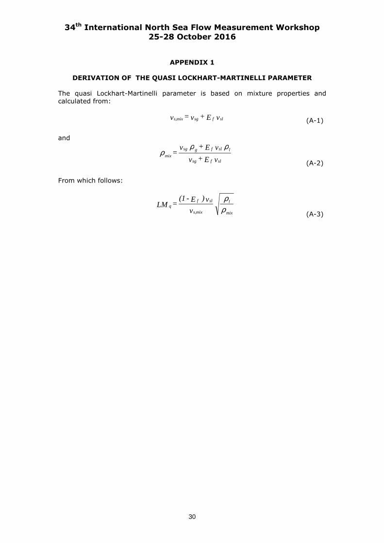
APPENDIX 1

DERIVATION OF THE QUASI LOCKHART-MARTINELLI PARAMETER The quasi Lockhart-Martinelli parameter is based on mixture properties and calculated from:

v E + v = v slfsgmixs, (A-1)

and

v E + v

v E + v =

slfsg

lslfgsg

mix

ρρρ

(A-2)

From which follows:

ρρ

mix

l

mixs,

slfq

v

v ) E - (1 = LM

(A-3)


31

APPENDIX 2

DISSIPATION DUE TO DRAG AROUND THE DROPLETS The droplets are accelerated in the convergent section and the throat of the Venturi and decelerated in the divergent part. The viscous forces which are responsible for these changes in velocity are also responsible for the dissipation of energy. This can be illustrated as follows: Imagine a steel sphere which is moving through a viscous fluid. After a while the sphere will reach its terminal velocity and in that case the forces of gravity and viscous drag are in balance. The dissipation will then equal the loss of potential energy of the sphere per unit time:

v F = mgv =

dt

dh

dh

d(mgh) =

dt

d(mgh) =

dt

dEee (B-1)

In the case of the droplets:

dE = dt )v - vF( ddg (B-2)

and

dt )v - v( F = E dgdd ∫

(B-3)

The force on the droplet is calculated as follows:

( )

2

1 r C = F d

2wd π

(B-4)

The drag coefficient is calculated by:

43 > Re 0.44 +

Re

24 = C d

dw

(B-5)

43 Re 1 = C dw ≤ (B-6)

in which Red is the Reynolds number of flow around droplet:

η

ρ

g

grrd

d v = Re

(B-7)

In order to calculate the Δp caused by this dissipation, the dissipation (which is calculated for an individual droplet) has to be multiplied by the number of droplets per m3 which can be found by calculating the number of droplets per second:

r

3

4E Q

= N3

flt

π (B-8)

and dividing this by the total volume flow rate:

(B-9)

Q + Q = Q glt


32

r

3

4 )Q + Q(

E Q = N

3gl

flv

π (B-10)

For the calculation, the diameter of the droplets is assumed to be equal to the average diameter in the pipe upstream of the Venturi. As soon as the fluids enter the Venturi, the gas will accelerate and thus exert a drag force on the droplet. As soon as the drag force exceeds the surface tension of the droplet, the droplet is assumed to split into two identical droplets. As the drag force on the droplet increases with the droplet diameter (due to the larger surface area and the larger inertia of the droplet) and the surface tension decreases with increasing droplet diameter (due to the reduced curvature, see also Appendix 3), the calculation of the droplet velocity is not very sensitive to the initial value of the droplet diameter: the forces on the droplet will result in droplets of similar diameter, virtually independent on the initial conditions.


33

APPENDIX 3

DIFFERENTIAL PRESSURE CAUSED BY SURFACE TENSION The droplets, dispersed in the gas, represent a potential energy, caused by the surface tension: in order to create a droplet, the surface tension has to be overcome. Imagine a m3 of liquid, split up into droplets with a diameter d (= 2r). The surface area of such a droplet is:

r4 = SA 2d π

(C-1)

The volume of such a droplet is:

r

3

4 = V 3

d π (C-2)

The m3 of entrained liquid thus yields a number of droplets equal to:

r

3

41

= N3

d

π (C-3)

The total surface area of the m3 entrained liquid is:

d

6 =

r

3 =

r3

4r4

= SA N = SA3

2

ddT

π

π

(C-4)

The pressure generated by the surface tension is:

σ

d

6 = Pst

(C-5)

However, the flow is two-phase, and thus the pressure is:

E

d

6 LVF = P factst,

σ

(C-6)

The reason is that the decrease in pressure is independent of the amount of liquid: if the fluid consisted of liquid only, the pressure decrease would be independent whether it was 1 ml or 1 m3. However, the smaller the fraction of liquid dispersed, the less the pressure decreases.

Documents

Modelling of Wet Gas flow in Venturi Meters to Predict the