Modelling of non-equilibrium turbulent flows Tania S. Klein Second Year PhD Student Supervisors: Prof. Iacovides and Dr. Craft School of MACE, The University

Modelling of non-equilibrium turbulent flows

Tania S. KleinSecond Year PhD Student

Supervisors: Prof. Iacovides and Dr. Craft

School of MACE, The University of Manchester

Outline of Presentation

Introduction

Test Cases

Turbulence

Models

Results

Conclusions

Introduction

Non-equilibrium flows: those subjected to rapid changes

Sudden contraction, sudden expansionImposed pressure gradients

They are commonly found in the industry:

Valves, pumps, heat exchangers, curve surfaces

Objective of this work:

Test different turbulence models for several cases in order to evaluate their performance.

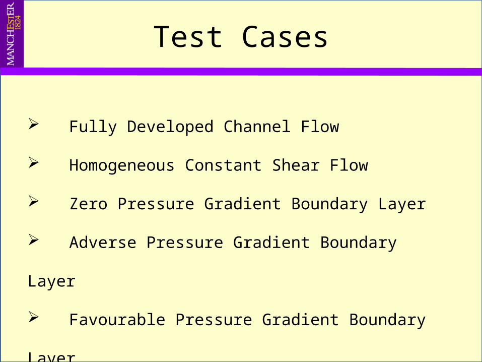
Test Cases

Fully Developed Channel Flow

Homogeneous Constant Shear Flow

Zero Pressure Gradient Boundary Layer

Adverse Pressure Gradient Boundary Layer

Favourable Pressure Gradient Boundary Layer

Contraction/Expansion Flows

Fully Developed Channel Flow

One of the simplest flows:

o 2Do P=cteo U=U(y)

Simulated Cases

ERCOFTACdatabase

Kawamura Lab

Homogeneous Constant Shear Flow

S=dU/dy=cte U = U(y) not wall-bounded

unsteady

Simulated Cases

Zero Pressure Gradient Boundary Layer

Still a simple flow:

o 2Do P=0o U=U(x,y)

Simulated Cases Rwhere data were evaluated

DNS of Spalart (1988) 300 670 1410

Experimental data of Smith (1994)

4981 13052 -

Adverse Pressure Gradient Boundary Layer

Non-equilibrium flow:

o 2Do P > 0o U=U(x,y)o dU/dx < 0

Simulated Cases

Samuel and Joubert (1974)

Marusic and Perry (1995)

S&J M&P

Favourable Pressure Gradient Boundary Layer

Non-equilibrium flow:o 2Do P < 0o U=U(x,y)o dU/dx > 0 o reaches a self-similar prolife

Simulated Cases Acceleration Parameter K

DNS of Spalart (1986) 1.5 x 10-6 2.5 x 10-6 2.75 x 10-6

Contraction/Expansion Flows

Non-equilibrium flow:

o 3Do dV/dy = cteo dW/dz = -cte

Simulated Cases

Tucker and Reynolds (1968)

Gence and Mathieu (1979)

= 0

= /2

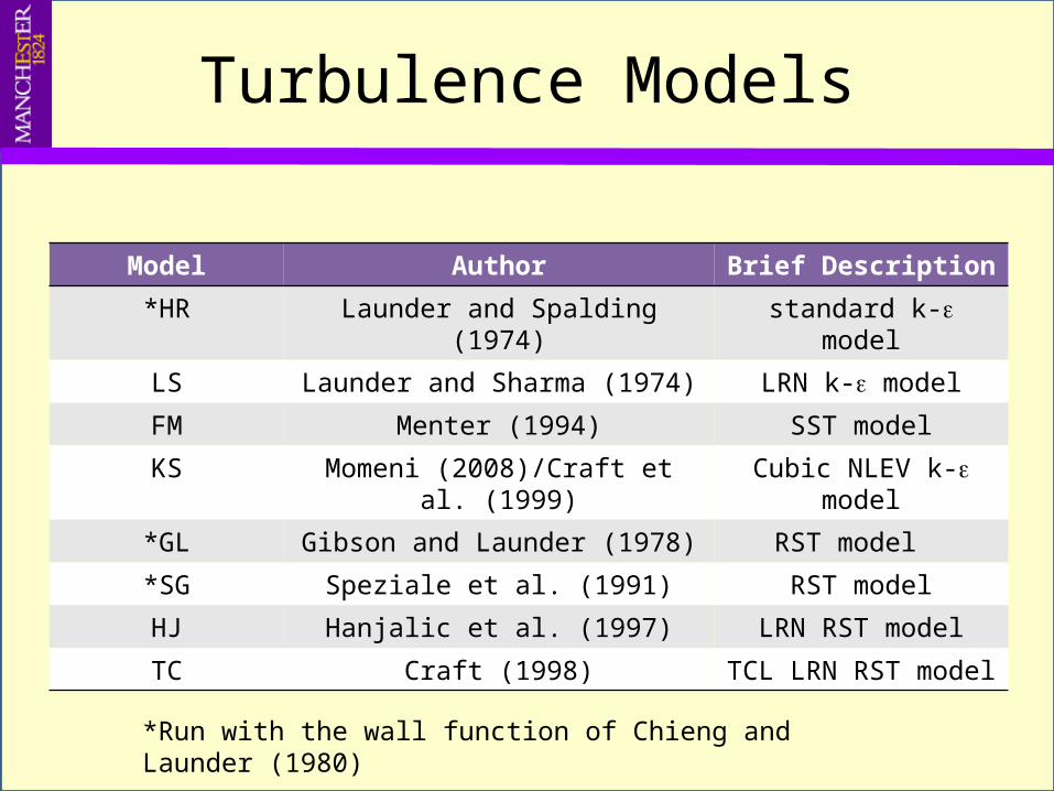
Turbulence Models

Model Author Brief Description

*HR Launder and Spalding (1974) standard k- model

LS Launder and Sharma (1974) LRN k- model

FM Menter (1994) SST model

KS Momeni (2008)/Craft et al. (1999)

Cubic NLEV k- model

*GL Gibson and Launder (1978) RST model

*SG Speziale et al. (1991) RST model

HJ Hanjalic et al. (1997) LRN RST model

TC Craft (1998) TCL LRN RST model

*Run with the wall function of Chieng and Launder (1980)

ResultsFully Developed Channel

FlowGeneral Conclusions

All models predicted the log law reasonably well.

All models predicted the shear Reynolds Stress reasonably

well.

The HJ and TC models best predicted the normal Reynolds

stresses.


FlowRe = 6500


FlowRe = 6500


FlowRe = 41441

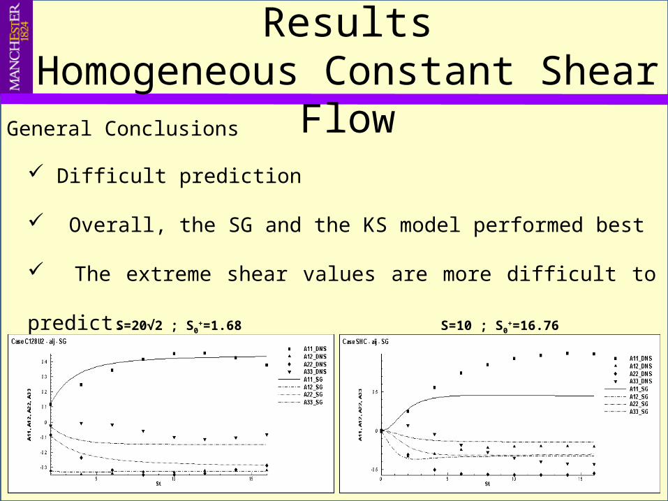
ResultsHomogeneous Constant Shear

FlowGeneral Conclusions

Difficult prediction

Overall, the SG and the KS model performed best

The extreme shear values are more difficult to predict.

S=20√2 ; S0+=1.68 S=10 ; S0

+=16.76


FlowS=20√2S0

+=1.68


FlowS=20√2S0

+=30.75

ResultsZero Pressure Gradient BL

General Conclusions

The tested turbulence models have shown to be sensitive to the inlet conditions, implying bad predictions at low Re values.

The normal Reynolds stresses were better predicted by the RST models, as expected.

One can notice the importance of LRN models for the near wall region predictions.



ResultsAdverse Pressure Gradient BL

General Conclusions

The BL parameters (Cf, , *, and H) were reasonably well predicted by all turbulence models.

The U and uv profiles were captured by all turbulence models up to station T5 in the S&J case. The same has not occurred for the M&P cases.

The RST models best predicted the normal Reynolds stresses, however the best model varies from case to case; station to station…


S&J


M&P


M&P

ResultsFavourable Pressure Gradient

BLGeneral Conclusions

The turbulence model which overall better predicted these flows was the KS model, although it failed to predict the Reynolds stresses.

The KS and LS models are the only ones expected to correctly predict the laminarization process, since they possess a term which accounts for the second derivative of the mean velocities.

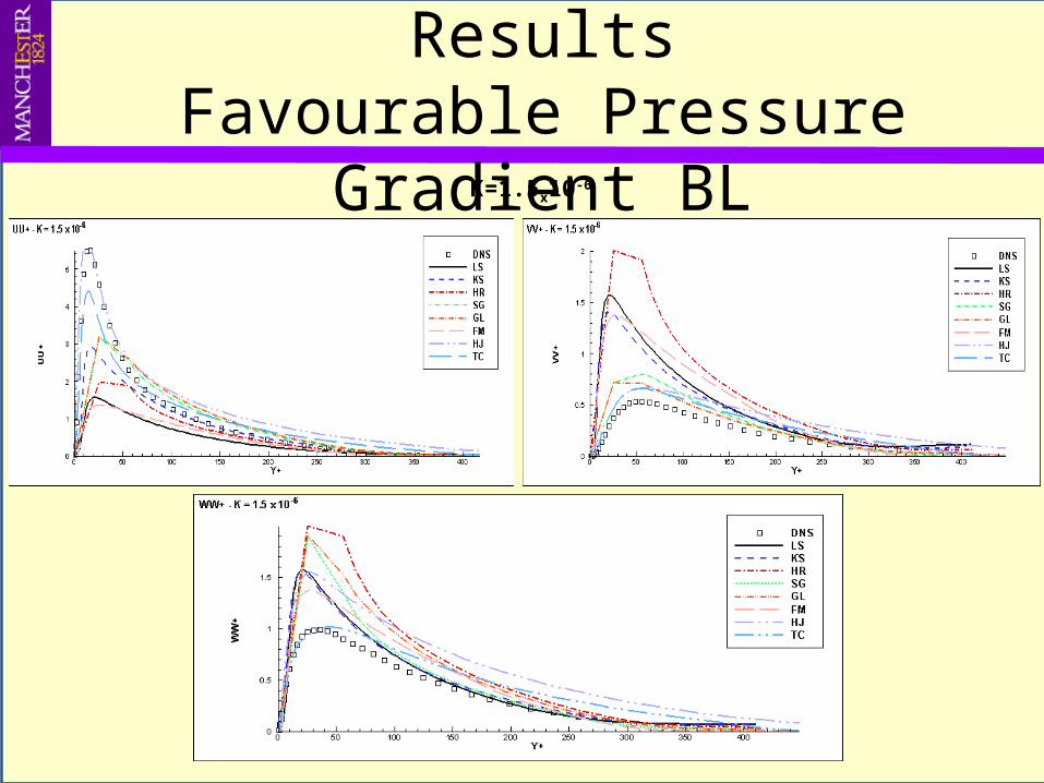
The RST models best predicted the normal Reynolds stresses, specially the TC and HJ models.


BLK=1.5x10-6


BLK=1.5x10-6


BLK=2.5x10-6


BLK=2.5x10-6

ResultsContraction/Expansion Flows

General Conclusions

No turbulence model was able to correctly predict the interruption of the applied strains.

Overall, the GL and the TC models provided the best predictions.

The eddy viscosity formulations clearly failed to predict these flows.

T&R



G&M - = /2

Conclusions

The Channel flow, which is the simplest flow, was reasonably well predicted by all turbulence models as well as the ZPGBL cases at high Re values.

The two not wall-bounded cases – HCS flow and C/E flows – were the most difficult to predict and the RST models performed better, showing the importance of calculating the Reynolds stresses through transport equations.

The APGBL cases could not be well predicted by any model at high P, however the FM model could match the U profile.

The FPGBL cases were better predicted by the KS model which evidenced the importance of a velocity second derivative term to predict laminarization.

Thank you

Documents

Modelling of non-equilibrium turbulent flows Tania S. Klein Second Year PhD Student Supervisors: Prof. Iacovides and Dr. Craft School of MACE, The University