Embed Size (px)
Citation preview

P O S I V A O Y
O l k i l u o t o
F I -27160 EURAJOKI , F INLAND
Te l +358-2-8372 31
Fax +358-2-8372 3709
Ve l i -Mat t i Pu lkkanen
Henr ik Nordman
March 2010
Work ing Repor t 2010 -14
Modelling of Near-Field Radionuclide TransportPhenomena in a KBS-3V Type of Repository for
Nuclear Waste with Goldsim Code – andVerification Against Previous Methods

March 2010
Working Reports contain information on work in progress
or pending completion.
The conclusions and viewpoints presented in the report
are those of author(s) and do not necessarily
coincide with those of Posiva.
Ve l i -Mat t i Pu lkkanen
Henr ik Nordman
V T T
Work ing Report 2010 -14
Modelling of Near-Field Radionuclide TransportPhenomena in a KBS-3V Type of Repository for
Nuclear Waste with Goldsim Code – andVerification Against Previous Methods

MODELLING OF NEAR-FIELD RADIONUCLIDE TRANSPORT PHENOMENA IN
A KBS-3V TYPE OF REPOSITORY FOR NUCLEAR WASTE WITH GOLDSIM CO-
DE - AND VERIFICATION AGAINST PREVIOUS METHODS
ABSTRACT
Traditional radionuclide transport models overestimate significantly some phenomena,
or completely ignore them. This motivates the development of new more precise models.
As a result, this work is a description of commissioning of a new KBS-3V near-field
radionuclide transport model, which has been done with a commercial software called
GoldSim. According to earlier models, GoldSim model usesrz coordinates, but the
solubilities of radionuclides have been treated more precisely.
To begin with, the physical phenomena concerning near-field transport have been in-
troduced according to GoldSim way of thinking. Also, the computational methods of
GoldSim have been introduced and compared to methods used earlier. The actual veri-
fication of GoldSim model has been carried out by comparing the GoldSim results from
simple cases to the corresponding results obtained with REPCOM, a software developed
by VTT and used in several safety assessments. The results agree well.
Finally, a few complicated cases were studied. In these cases, the REPCOM’s limitations
in handling of some phenomena become evident. The differences in the results are caused
especially by the extension of the solubility limit to the whole computational domain, and
the element-wise treatment of the solubilities which was used instead of nuclide-wise
treatment.
This work has been carried out as a special assignment to the former laboratory of Ad-
vanced Energy Systems in Helsinki University of Technology. The work was done at
VTT.

RADIONUKLIDIEN LÄHIALUEEN KULKEUTUMISILMIÖIDEN MALLINN US
KBS-3V LOPPUSIJOITUSTILASSA GOLDSIM MALLILLA - JA VERIFIOINTI
AIKAISEMPIIN MENETELMIIN VERRATEN
TIIVISTELMÄ
Perinteiset radionuklidien kulkeutumismallit yliarvioivat reilusti joitakin ilmiöitä tai jät-
tävät ne kokonaan huomiotta. Tämä motivoi uusien tarkempien mallien kehittämistä.
Tässä työssä kuvataankin uuden GoldSim ohjelmalla tehdyn KBS-3V konseptin mu-
kaisen radionuklidien lähialuekulkeutumismallin käyttöönotto. Aikaisempien mallien ta-
paan GoldSim mallissa käytetäänrz-koordinaatistoa, mutta radionuklidien liukoisuusra-
joitteisuus on käsitelty aiempaa tarkemmin.
Aluksi radionuklidien kulkeutumiseen liittyvät ilmiöt onkuvattu GoldSimin ajatusmal-
lin mukaisesti, laskennalliset menetelmät on esitelty ja näitä on verrattu aiemmin käy-
tettyihin menetelmiin. Varsinainen GoldSim mallin verifiointi on suoritettu vertaamalla
yksinkertaistetuista tilanteista saatuja tuloksia REPCOM-ohjelmalla saatuihin vastaaviin
tuloksiin. REPCOM on VTT:n kehittämä useissa turvallisuusanalyyseissa käytetty ohjel-
ma. Tulokset vastaavat toisiaan hyvin.
Lopuksi yksinkertaisista tilanteista on siirrytty mutkikkaampiin, joissa perinteisen
REPCOM mallin rajat ilmiöiden käsittelyssä tulevat vastaan. Eroja tuloksiin aiheuttavat
erityisesti uudessa mallissa tehtävä liukoisuusrajojen ulottaminen koko laskenta-alueelle
ja rajojen käsitteleminen alkuainekohtaisesti nuklidikohtaisen käsittelyn sijaan.
Tämä työ on tehty erikoistyönä Teknillisen korkeakoulun entiseen Energiatieteiden labo-
ratorioon. Työn tekopaikkana toimi VTT.

1
TABLE OF CONTENTS ABSTRACT TIIVISTELMÄ
1 INTRODUCTION ................................................................................................. 3
2 BACKGROUND ................................................................................................... 4
2.1 Actors in Nuclear Waste Management. ....................................................... 4
2.2 The State of the Finnish Disposal Plan ....................................................... 4
2.3 Radionuclide Transport Computation at VTT. ............................................. 5
3 PHYSICAL PHENOMENA. .................................................................................. 7
3.1 Sorption and Retardation in a Porous Medium ............................................ 7
3.2 Diffusion through a Porous Medium .......................................................... 10
3.3 Solubility Limits ......................................................................................... 11
3.4 Radioactive Decay .................................................................................... 11
3.5 Connecting the Phenomena. .................................................................... 12
4 COMPUTATIONAL METHODS. ........................................................................ 13
4.1 The Approach to the Mass Transport Problem. ......................................... 13
4.2 Discretizing the Diffusion. ......................................................................... 13
4.3 Dealing with Nonlinearity when a Solubility Limit is Reached .................... 14
4.4 The Cell Net Solution Algorithm ................................................................ 16
4.5 Solving the Linear Equations .................................................................... 17
4.6 The REPCOM Approach........................................................................... 17
5 DEVELOPING THE TRANSPORT MODEL ....................................................... 19
5.1 The Geometry ........................................................................................... 19
5.2 The Step by Step Developing Strategy. .................................................... 19
5.3 The Tests with the Stable Verification Nuclides ........................................ 21
5.4 A Simple Decay Chain with Shared Solubilities. ....................................... 25
5.5 Several Chains Computed Simultanously. ................................................ 26
6 DISCUSSION .................................................................................................... 30
6.1 Comparing GoldSim and REPCOM. ........................................................ .30
6.2 Future Prospects. ..................................................................................... 30
REFERENCES ........................................................................................................... 32
APPENDICES............................................................................................................. 34

2
A GRID AND TIMESTEP DETAILS ....................................................................... 34
B RADIONUCLIDE AND MATERIAL PROPERTIES. ............................................ 36
C THE CONTENTS OF THE WASTE. .................................................................. 37
3
1 INTRODUCTION
Nuclear energy has been powering the Finnish industry and households over three decades.
During this time, spent fuel has accumulated in the intermediate storages nearby the
power plants. The Finnish final disposal plan for spent fuel is, in brief, to seal the fuel
rods into iron-copper canisters, surround the canisters with bentonite, a clay-like well-
expanding, diffusion-dominating material, and place the whole package approximately
half kilometer deep into the bedrock. The idea sounds simplebut the planning and the
execution are quite demanding. Due to the long-lasting radioactive waste material and
the public image of nuclear power, the research on disposal must be thorough and ex-
tensive as well as intelligible to authorities and public. The licensing of such a geologic
repository for spent fuel requires, among other things, a safety case, that is, a summary of
all arguments that show that there is reasonable assurance that the spent fuel management
solution remains safe for a long time.
The regulatory requirements for a spent fuel repository at Olkiluoto are set out in the
Government Decision on the safety of the disposal of spent nuclear fuel (STUK, 1999)
and, in more detail, in Guide YVL 8.4 issued by the Finnish regulator STUK (2001).
These requirements are, however, currently under revision. Guide YVL 8.4 distinguishes
between the "environmentally predictable future" (also referred to by the regulator as
"several thousand years"), during which conservative estimates of dose must be made (i.e.
estimates that tend to over-estimate dose where there is uncertainty), and the "era of large-
scale climate changes" when periods of permafrost and glaciations are expected, and
radiation protection criteria are based on constraints on nuclide-specific activity fluxes
from the geosphere, termed "geo-bio flux constraints". YVL 8.4 also gives a qualitative
requirement that: "The barriers shall effectively hinder the release of disposed radioactive
substances into the host rock for several thousands of years."
This report focuses on the radionuclide release and transport model in a case of an early
canister failure, which is very unlikely.

4
2 BACKGROUND
2.1 Actors in Nuclear Waste Management
To understand the context and the needs the modelling is facing, a brief introduction to
the circumstances of nuclear waste management in Finland isneeded. In Finland, the
spent fuel disposal is managed by Posiva Oy. It is owned and funded by the energy
corporations Fortum Oy and Teollisuuden Voima Oy that produce nuclear energy. Posiva
carries out research on its own or contracts it out to external organisations, such as VTT,
Technical Research Centre of Finland. The third party on thedisposal field is STUK,
the Radiation and Nuclear Safety Authority. It regulates the safety of handling, storage
and disposal of nuclear waste. The Ministry of Employment and the Economy handles
the general regulation of the final disposal, decides on principle and establishes the time
schedules to be implemented by the power companies. A schematic presentation of the
counterparties is shown in Figure 2-1.
Finnish Government|
Ministry ofEmployment and
the Economy
Radiation andNuclear
Safety Authority
TeollisuudenVoima Oy
|
FortumPower and Heat Oy
|
POSIVA OY
|Posiva’s network of partners:research institutes, universities,
consultants, contractorsVTT ��3
-Supervision
-Legislation
Licenses
Figure 2-1. The main Finnish nuclear waste management actors and their relations. Thepicture is a replica of a picture at Posiva’s homepage (POSIVA, 2008) with additionalVTT text.
2.2 The State of the Finnish Disposal Plan
The Finnish disposal plan, touched briefly in the introduction, is presented in schematic
pictures in Figure 2-2. Due to the political consensus, the Finnish plan has evolved into

5
Figure 2-2. A picture series of the disposal site. The Finnish plan follows essentiallythe Swedish KBS-3V plan and the picture series is from a Swedish technical report (SKB,2006b).
quite a mature state. The next grand step is to apply a construction license to dispose the
nuclear waste. Posiva plans to submit the application to STUK in 2012. Not surprisingly,
the planning and the research of the disposal is speeding up.At the same time, new
modelling tools arise and computational capabilities improve. As a result, more realistic
and developed models are wanted. However, the models have tobe kept simple enough so
that they can be interpreted clearly. To meet these challenges in the field of radionuclide
transport, VTT has introduced a new simulation program called GoldSim, the main object
of this report.
2.3 Radionuclide Transport Computation at VTT
The principle of conservativeness is used when computatingthe release of the disposed
radionuclides. It means that all simplifying estimates should be made in a way that they
do not underestimate the effects of the release.
At VTT, the radionuclide transport from the repository to biosphere has mostly been
computed with a in-house code called REPCOM, REPository COMpartments. It has
been programmed withfortran77 and is rather old, but it works fine, especially with
modern computers. However, it makes some overly conservative estimates that mask
some significant phenomena. The present-day tendency to make the estimates as real as
possible without loosing the conservativeness is not really followed. One more obstacle

6
preventing the widespread usage of REPCOM is the unclarity of the user interface.
Some tests have been made with a program called PORFLOW to confirm the calculations
made with REPCOM. The results obtained with the programs coincide well and have
been published in the technical report (Nordman and Vieno, 2003).
For further information about the radionuclide transport computing at VTT, contact REP-
COM specialist Lic.Sc. Henrik Nordman or get acquainted with the technical reports
(Nordman and Vieno, 2003), (Nordman and Vieno, 1994), and (Vieno and Nordman,
2000).

7
3 PHYSICAL PHENOMENA
3.1 Sorption and Retardation in a Porous Medium
Porous materials tend to react with nuclides by sorbing themon surfaces. The degree of
sorption is described by the distribution coefficient1 Kd, which is defined as
Kd =ms/Ms
mf/Vf(1)
where
Kd = the distribution coefficient (m3/kg)ms = the mass of the nuclide sorbed on the solid material (kg)Ms = the mass of the solid material (kg)mf = the mass of the nuclide in the fluid (typically water) (kg)Vf = the volume of the fluid (m3).
Partition coefficient can also be defined between two fluids ortwo solids. If the volumes
of fluids and the masses of solids are denoted with quantitiesU , Equation (1) becomes
K1,2 =m1/U1
m2/U2(2)
K1,2 = the distribution coefficient betweenmaterials 1 and 2 (m3/kg or kg/m3 or -)
mi = the mass of the nuclide in materiali (kg)Ui = the quantity of the materiali, m for solids
andV for fluids (kg or m3).
For computational purposes, it is useful to define a reference fluid which all the other
materials are compared to. This is what GoldSim does and, thus, the following notation is
adopted from the GoldSim user’s guide (GoldSim, 2007). For each substance a partition
coefficientKmaterial,ref can be expressed vis-à-vis the reference fluid. Consequently,
the partition coefficient between two substances can be calculated from their reference
partition coefficients:
K1,2 =K1,ref
K2,ref
. (3)
In addition, the units of the reference partition coefficients have units [volume]/[mass]
for solids and [volume]/[volume] for fluids. If, again, the volumesV ’s and the masses
1The distribution coefficient is also called a partition coefficient.

8
M ’s are referred as quantitiesU of medium corresponding the partition coefficients, the
concentration of the nucliden in materiali is
cn,i =Ki
∑
j (KjUj)mn (4)
where
cn,i = the concentration of the nucliden in materiali (kg/m3)Ki = Kd between materiali and the reference fluid (m3/kg, kg/m3 or -)Kj = Kd between materialj and the reference fluid (m3/kg, kg/m3 or -)Uj = the quantity of the materialj (kg or m3)mn = the mass of the nucliden in the volume (kg).
The summation is taken over all the materials in the volume. In this report, all the vol-
umes contain only water and single solid material. Thus, theconcentration in water can
be calculated usingKd from Equation (1) in Equation (4). However, for further use of
the model the above general form of concentration used by GoldSim is introduced.
Retardation of the mass transport through a medium, caused by the sorption and the
pores, is specified by the retardation factorR:
R =mt
mf
=ms + mf
mf
(5)
where
R = the retardation factor (-)mt = the total mass of an element (kg)mf = the mass of an element in the fluid (kg)ms = the mass of an element in the solid (kg).
In a porous material, the retardation factor is
R =mt
mf= 1 +
ms
mf= 1 +
MsKd
Vf= 1 +
(1 − ε)VtρsKd
εVt= 1 +
1 − ε
ερsKd (6)
where

9
ε = the porosity2of the material (-)mt = the total mass of an element (kg)mf = the mass of an element in the fluid (kg)ms = the mass of an element in the solid (kg)Ms = the mass of the solid (kg)Kd = the distribution coefficient (m3/kg)Vf = the volume of the fluid (m3)Vt = the total volume (m3)ρs = the dry density of the solid (kg/m3).
(Nordman and Vieno, 1994) (GoldSim, 2007)
2Geometrically seen, porosity is the percentage of the pore volume in a material. However, in somecases all the pore volume is not available for some substances. For example, anion exclusion reduces thespace for anions in clay. In these cases, the porosity shouldbe considered rather as a diffusion relatedparameter than as a pure geometric property.

10
3.2 Diffusion through a Porous Medium
In a simple fluid, the diffusion obeys Fick’s law
~jf = −Df∇cf (7)
where
~jf = the mass flux3of the substance in a fluidf (kg/(m2·s))
Df = the diffusion coefficient (m2/s)cf = the concentration of the substance in the fluidf (kg/m3)∇ = gradient operator.
In a porous media, the geometry complicates the diffusion and the equation takes the
form
~jporous = ǫδ
τ 2~jf = −ǫ
δ
τ 2Df∇cf = −ǫGDf∇cf = −De∇cf (8)
where
~jporous = the mass flux in the porous media (kg/(m2·s))
δ = the constrictivity (-)τ = the tortuosity (-)G = the factor denoting the geometric properties
of the pores on diffusion4 (-)ε = the porosity (-)Df = the diffusion coefficient of the fluid (m2/s)De = the effective diffusion coefficient of the fluid
in the medium (m2/s).
The mass flow through a surfaceS is obtained by integrating the previous equation over
the surface, i.e.
m = −
∫
S
De∇cf · ~ndS (9)
where~n is the normal vector of the surface.
3As distinct from molic flux presented by capital~J , the mass flux is denoted by lower case~j. Of course,in the molic flux case, also the concentration should be presented in moles.
4GoldSim uses tortuosityτ in the place ofG. This should be noted to avoid mistakes.

11
3.3 Solubility Limits
When an element is dissolved in a fluid, sometimes its concentration is limited by its
solubility. The limit is called the solubility limit. If theamount of the element in a volume
is more than what can be dissolved, the exceeding part precipitates. The solubility limit is
an element property. Thus, the isotopes of an element share the solubility in the isotopic
ratio, and this complicates the mass transport computationa bit.
GoldSim uses mass transport approach, and thus the following equation is needed. Given
a volumeV , the amount of element saturating the fluid ismsat. It can be determined by
msat = nr∑
i
KiUi (10)
where
msat = the mass of the element causing the saturationin the volume (kg)
nr = the solubility limit of the reference fluid (mol/l)Ki = Kd between materiali and the reference fluid (m3/kg, kg/m3 or -)Ui = the quantity of the materiali, m for solids
andV for fluids (kg or m3).
The summation is taken over all the mediums in the volumeV .
3.4 Radioactive Decay
The well-known differential equation for radioactive decay for some nuclide is
N = −λN (11)
where
N = the number of the radioactive nuclei (-)N = the time derivative ofN (1/s)λ = the decay constant (1/s).
The half-life of a nuclide can be derived from:
T1/2 =ln2
λ. (12)
Equation (11) can be written with respect to the mass of a nuclide:

12
m = −λm (13)
where
m = the mass of a nuclide (kg)m = the time derivative ofm (kg/s).
When a radionuclide decays, it becomes another nuclide, called a daughter nuclide. If an
overall mass change of the nuclidei due to the radioactive decay is wanted, the rate of
mass change becomes
mi = −λimi +∑
j
fjRjAi
Ajλjmj (14)
where
λi = the decay constant of nuclidei (1/s)fj = the fraction of the parent nuclidej that decays
to the nuclideiRj = the stoichiometric ratio of moles of nuclidei
produced per mole of nuclidej decayed (1/s)Ai = the atomic weight of the nuclidei (g/mol)
The summation is taken over all the direct parent nuclides ofthe nuclidei.
If a heavy radionuclide decays to a daughter nuclide, the daughter tends to decay further.
Nuclides of this nature form specific decay chains. However,for computational purposes,
it is practical to define a bit larger concept, a decay family.Simply, it consists of all the
decay chains that have nuclides of common elements.
3.5 Connecting the Phenomena
All the preceeding mass change rates can be combined into oneequation. If a volumeV
is considered, the mass change rate is
mV = −λimi +∑
j
fjRjAi
Ajλjmj −
∫
∂V
De∇cf · ~n dV + S (15)
where Equations (14) and (9) have been combined, and a sourcetermS has been added.

13
4 COMPUTATIONAL METHODS
This section is a description of the mass transport solving techniques that GoldSim is
based on5 . The methods used in REPCOM are also discussed here.
4.1 The Approach to the Mass Transport Problem
GoldSim uses a control or finite volume approach to solve the mass transport problem
of the radionuclides. The idea is to divide the region examined in small volumes and
compute the mass changes in them. The small volumes are oftencalled control or finite
volumes, but the GoldSim uses the term cell. Consequently, the term cell is also used in
this report. Further, the computational region, i.e. the cells, is called cell net. The mass of
a nuclide in a cell can change by diffusion to the neighbouring cells, by radioactive decay,
or by the radioactive decay of the parent nuclides. These phenomena are described by
applying Equation (15) to each cell and discretizing the diffusion. Of course, the obtained
equations have to be discretised also timewise. In a cell, the mixing and the sorption of
the nuclides is assumed to happen instantaneously. The cellnet uses cylindrical geometry
without angular dependency.
4.2 Discretizing the Diffusion
When the solubility limit is not reached, the diffusive massflow for a nuclide from a cell
i to a neighbouring cellj is
md,i→j = Qi→j
(
ci −cj
Kji
)
(16)
where
ci = the dissolved concentration of a nuclide in the celli (kg/m3)Qi→j = the diffusive conductance between the cellsi andj (m3/s)Kji = the distribution coefficient between the fluids
in the cellj andi (-).
The diffusive conductance of the celli in thei → j direction with a simple discretization
of the diffusion6 is
Qi,i→j =De,iA
∆xi(17)
5For further details of the GoldSim techniques, see the GoldSim manual (GoldSim, 2007)6The discretazion takes only the nearest neighbours into account. In the orthogonal uniformxy-
coordinates this equals central difference with truncation errorO(∆x2, ∆y2) (Siikonen, 2006)

14
where
A = the diffusive area (m2)∆xi = the diffusive lenght in the celli (m)De,i = the effective diffusion coefficient in the celli (m2/s).
The diffusion conductance in the cellj has the same form. Consequently, these conduc-
tances in series are the conductance between the cells,
Q =A
∆xi
De,i+
∆xj
De,j
. (18)
The mass flow in Equation (16) can be divided into two parts, one of which is dependent
only of the mass in the celli and drives mass from the celli to j. Correspondingly, the
other drives mass from cellj to i and depends only on the mass in cellj. In other words,
the unidirectional diffusive mass flow is calculated assuming that the concentration in
the other cell is zero. The sum of two opposite unidirectional flows equals the whole
mass flow. According to this idea, a unidirectional diffusive flow for a nuclidefi→j is
introduced as
fi→j = tdi→jmi (19)
wheretdi→j is a transfer coefficient for dissolved nuclide from celli to j specified by the
diffusive conductance in Equation (18) and the distribution coefficients of the nuclide in
question between materials in cellsi andj.
4.3 Dealing with Nonlinearity when a Solubility Limit is Rea ched
When the solubility limit is reached, the unidirectional diffusive flow in Equation (19)
becomes
fi→j = tdi→j
nsi
ni
mi (20)
tdi→j = the transfer coefficient (1/s)mi = the mass of the nuclide (kg)ni = the total amount of the element in the celli (mol)ns
i = the solubility limit of the element in the celli (mol).
The equation is non-linear and to solve it, GoldSim applies the first order Taylor expan-
sion at reference points that are chosen to meet the accuracydemands. If the values at a

15
reference point are denoted by an overline (m, n) and the cell indexes are dropped, the
first order expansion of Equation (20) is
f ≈ tdns
nm + tdns
∑
iso
[
∂
∂miso
(m
n
)
ref(miso − miso)
]
(21)
where
tdi→j = the transfer coefficient (1/s)m = the mass of the nuclide (kg)n = the total amount of the element (mol)ns = the solubility limit of the nuclide (mol)miso = the mass of a isotope of the same element
as the nuclide that is being computed (kg).
The summation takes all the isotopes of the element into account and the derivatives are
evaluated at the reference point. The summation term can be further expanded as
∑
isotopes
[
∂
∂miso
(m
n
)
ref(miso − miso)
]
=ms − ms
n−
m
n2
∑
isotopes
miso − miso
Mr,iso
=ms − ms
n−
m
n2
∑
isotopes
miso
Mr,iso
+m
n(22)
whereMr denotes the molecular weight. With the summation (22) and rearranging, the
original Equation (21) can be written as
f ≈ (m + m) tdn
n− m td
n
n2
∑
isotopes
miso
Mr,iso
. (23)
GoldSim uses Equation (19) to calculate the mass transport from cell to another whenever
possible. However, at some point the solubility limit is reached and the program has to
switch to Equation (23) to calculate the diffusion. The problem is when to change the
equation. If the time-step is too long, the solubility limitis exceeded which is physically
not realistic. To avoid the unrealistic result, GoldSim uses fractional time-stepping when
the limit is approached. It shortens the time-steps so that the change is made time-wise
reasonably precisely. With high precision settings the maximum solubility overshoot is
2.5 per cent, and the shortest time-step is 10−8th of the user specified step. For further
information about the precision settings, see appendix A.

16
4.4 The Cell Net Solution Algorithm
When the discretized unidirectional diffusive flows are applied to the whole region, the
mass change Equation (15) for one nuclide can be expressed ina matrix form. However,
because of the decay properties and the element nature of thesolubility, a whole decay
family has to be solved at once. If the masses of each nuclide in each cell are arranged
into a vectorm, an equation
m = [D + T ] m + S (24)
is obtained. The symbols are
m = vector containing the masses of each nuclide of a decay family ineach cell
m = the time derivative ofmD = the matrix which all the decay and ingrowth coefficients7
T = the matrix which contains the mass transfer coefficients between thecells, i.e. the same coefficients as in the unidirectional diffusionequations (19) and (20). Also, direct flow rates can be given to thecells with the mass transfer coefficients, for example, forboundary condition purpose.
S = the vector containing the sources of the nuclides.
GoldSim solves Equation (24) with implicit Euler method, also called first order back-
wards difference formula if looked from another point of view. 8 The method applied to
Equation (24) gives
m(t + ∆t) − m(t)
∆t= [D + T ] m(t + ∆t) + S(t) (25)
where∆t is a time-step. A basic form of Equation (25) is
[I − D∆t − T∆t] m(t + ∆t) = m(t) + S(t)∆t (26)
whereI is the identity matrix. The length of them vector for a decay family is m×n
where m is the number of the nuclides and n is the number of the cells in the cell net. In
consequence, the size of the matricesI, D, andT is (m×n)×(m×n).
7The ingrowth coefficients express the rate at which the parent nuclides decay to the daughters.8The method is unconditionally stable and conserves mass. For further information about the method,
consult any proper book on numerical solutions of partial orordinary differential equations, for example(Smith, 1985), (Larsson and Thomée, 2003), or (Burden and Faires, 1983).

17
4.5 Solving the Linear Equations
Solving the sparse matrix Equation (26) is a matter of numerical linear algebra. GoldSim
uses a two-step, fail-safe approach with iterative methods. Firstly, it solves the system
with the Bi-Conjugate Gradient Stabilized method, BiCGS. If the method fails for any
reason, Generalized Minimum RESidual method, GMRES, is applied. BiCGS is a robust
and efficient method, but not as robust and general as the GMRES. However, BiCGS is
preferred to GMRES as the solution method, because GMRES is somewhat slower. For
further information about the linear algebra, see books (Barrett et al., 1994), (Trefefen
and Bau III, 1997), and webpage (IML++, 2008).
4.6 The REPCOM Approach
This section is a quick review of the methods included in REPCOM for comparison.
REPCOM uses the same kind of diffusion model as GoldSim, i.e.the radionuclides dif-
fuse to the neighbouring compartments (cells) with a rate specified by the concentration
difference, diffusive length, area, and coefficient. However, REPCOM does not take the
solubility limits into account outside the disposal canister. Also, the decay chains are
computed separately. Consequently, the solubility is treated as a nuclide-specific prop-
erty, even though, strictly speaking, it is an element-specific property. These nonrealistic
simplifications may lead to too fast release rates, and so, they are the main reasons to
change REPCOM to GoldSim as a modelling tool. With the simplifications, the equation
to be solved takes the form
dA
dt= B A(t) + S(t) (27)
where
A = the the vector containing the nuclide inventories in the compartmentsB = the diffusive coefficient matrixS = the vector containing the nuclide sources.
REPCOM solves this equation in an unusual manner. It uses thewell-known analytical
solution
A(t) = eB·(t−t0)A(t0) +
∫ t
t0
eB·(t−τ)S(τ)dτ (28)
to the ordinary differential equation, Eq. (27), and calculates the matrix powers with the
eigenvalue decomposition. This is contrary to conventional methods that solve Equation

18
(27) directly. The eigenvalues and -vectors are calculatedwith LAPACK’s dgeev 9
subroutine. The computational cost of finding all the eigenpairs of a large matrix is
considerable compared to solving an equal size linear equation. In consequence, the
method based on the eigenvalue decomposition is not recommended for large problems.
In principle, the exponential of a matrix could be computed in many ways. Methods
involving approximation theory, differential equations,the matrix eigenvalues, and the
matrix characteristic polynomial have been proposed. In practice, consideration of com-
putational stability and efficiency indicates that some of the methods are preferable to
others, but that none are completely satisfactory (Moller and Van Loan, 1978). In a
repository for a nuclear waste the transport of radionuclides is however dominated by
diffusion. It has been noticed that the method used by REPCOMworks well in these
kind of cases. Several verifications against analytical formulas or other computer models
have confirmed this.9LAPACK = Linear Algebra PACKage provided, for example, by webpage (LAPACK, 2008). To
understand the methods LAPACK uses, consult any proper bookconcerning numerical linear algebra, forexample (Trefefen and Bau III, 1997).

19
5 DEVELOPING THE TRANSPORT MODEL
5.1 The Geometry
A schematic presentation of the modelled deposition hole isshown in Figure 5-1. The
damage of the canister is assumed to be severe, and it is presented as a 35 cm high missing
part of the canister at the top of it. The part corresponds theinner wall of the buffer block
B1. In the model, ground water flows in a rock fracture spreading into the disturbed
rock zone next to outer wall of the buffer block B1. The equivalent rate of this flow
is denoted withQF . Respectively, the equivalent ground water flows from the backfill
in the deposition hole and the tunnel section areQDZ andQTDZ , respectively. Some
conservative assumptions are made, like the half a meter high missing buffer part under
the canister. The geometry and some data of the deposition environment in numbers are
presented in Table 5-1. The material properties of the real nuclides have been compiled
in Appendix B. In all the computed cases, the bedrock environment is non-saline and all
the values of the properties follow this assumption.
5.2 The Step by Step Developing Strategy
To make sure that the model under introduction will work properly, a careful step-by-
step developing strategy is used. The idea is to include eachnew property in the model
one by one, and compare the new results to the reference results obtained with another
model. In this case, GoldSim is developed according to the strategy with REPCOM as a
reference model. The REPCOM results were computed by HenrikNordman, following
the approach described in (Nordman and Vieno, 2003).
QDZ
Canister interior
QTDZ
QF
Tunnel Section
B2
B3
B1
Bentonite buffer
Tunnel backfill
Figure 5-1. A side view of the modelled deposition hole (Nordman and Vieno, 2003).
20
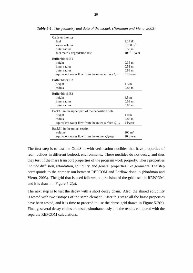
Table 5-1. The geometry and data of the model. (Nordman and Vieno, 2003)
Canister interiorfuel 2.14 tUwater volume 0.700 m3
outer radius 0.53 mfuel matrix degradation rate 10−6 1/year
Buffer block B1height 0.35 minner radius 0.53 mouter radius 0.88 mequivalent water flow from the outer surfaceQF 0.2 l/year
Buffer block B2height 1.5 mradius 0.88 m
Buffer block B3height 4.5 minner radius 0.53 mouter radius 0.88 m
Backfill in the upper part of the deposition holeheight 1.0 mradius 0.88 mequivalent water flow from the outer surfaceQDZ 2 l/year
Backfill in the tunnel sectionvolume 100 m3
equivalent water flow from the tunnelQTDZ 10 l/year
The first step is to test the GoldSim with verification nuclides that have properties of
real nuclides in different bedrock environments. These nuclides do not decay, and thus
they test, if the mass transport properties of the program work properly. These properties
include diffusion, retardation, solubility, and general properties like geometry. The step
corresponds to the comparison between REPCOM and Porflow done in (Nordman and
Vieno, 2003). The grid that is used follows the precision of the grid used in REPCOM,
and it is drawn in Figure 5-2(a).
The next step is to test the decay with a short decay chain. Also, the shared solubility
is tested with two isotopes of the same element. After this stage all the basic properties
have been tested, and it is time to proceed to use the dense grid drawn in Figure 5-2(b).
Finally, several decay chains are tested simultaneously and the results compared with the
separate REPCOM calculations.

21
0 0.2 0.4 0.6 0.8 10
1
2
3
4
5
6
7
8
r (m)
z (m
)
0 0.2 0.4 0.6 0.8 10
1
2
3
4
5
6
7
8
r (m)
z (m
)
(a) the coarse grid (b) the dense grid
Figure 5-2. The grids inrz-coordinates. The details of the grids can be seen in AppendixA. The bold lines on the outer edge present the flow boundary conditions caused by theequivalent flowsQF and QDZ . The inner bold line denotes the length of the canisterwhere the damage has occurred, i.e. there is no wall at that location. The uppermostcells with the upper wall at height 7.3 m neighbour the tunnelwhere the nuclides candiffuse. The tunnel is modelled as a separate volume, and theequivalent flow from thetunnel isQTDZ . All the other boundaries are impenetrable. The diffusive lengths in thecanister and in the tunnel have been conservatively estimated to be negligible, i.e., zeros.
5.3 The Tests with the Stable Verification Nuclides
The stable verification nuclides are of different types: non-sorbing neutral N-S, sorbing
neutral S, anion A, and cation C. The material properties forthese nuclides are shown
in Table 5-2. Two tests were performed for these nuclides. Inthe first one, an instant
release of one mole of each nuclide without solubility limits was simulated. The release
rate from the near-field, i.e. the rate the nuclides diffuse to the flowsQF , QDZ , and
QTDZ, is plotted in Figure 5-3(a). The second test probes the performance of GoldSim in
presence of solubility-limited species. The solubility islimited to 1 mol/l for all nuclides,
and the instant release is 109 moles to make sure that the solubility is limited inside the
canister from the beginning. The results are presented in Figure 5-3(b). For the non-

22
Table 5-2. The verification nuclides
N-S S A C
Speciation Neutral Neutral Anion Cation
Buffer (non-saline)Kd (m3/kg) 0 0.3 0 0.018ε 0.43 0.43 0.17 0.43De (m2/s) 1.2·10−10 1.2·10−10 1·10−11 3·10−10
Backfill (non-saline)Kd (m3/kg) 0 0.3 0 0.0061ε 0.23 0.23 0.23 0.23De (m2/s) 2·10−10 2·10−10 2·10−10 2·10−10
solubility-limited case, the maximum rates and their timesof occurence can be found in
Table 5-3. Also, the equilibrium rates in the limited case have been collected into the
same table.

23
100
102
104
106
10−8
10−7
10−6
10−5
10−4
10−3
The pulse with verification nuclides
time (year)
rele
ase
rate
(B
q/ye
ar)
NSSAC
(a)
100
102
104
106
10−4
10−3
10−2
10−1
100
101
Solubility limited verification nuclides
time (year)
rele
ase
rate
(B
q/ye
ar)
NSSAC
(b)
Figure 5-3. The result with the verification nuclides. The solid lines present the GoldSimresults and the dashed line the REPCOM results. The upper figure is the 1 mole instantrelease case without solubility limit. The lower figure is the solubility limited case withthe large instant release. Some minor differences can be observed especially at the mid-stages of the plots.

24
Table 5-3. The maximum rates and the maximum times for the case with no the solubilitylimits as well as the limits and the times when 90 per cent of the limits are reached forthe limited case.
The non-solubility-limited case withone mole inside canister att=0
time (year) maximum (mol/year)
nuclide GoldSim REPCOM GoldSim REPCOM
N-S 7.29·102 6.30·102 2.34·10−4 2.33·10−4
S 3.99·103 4.36·103 4.19·10−7 4.10·10−7
A 1.24·103 1.20·103 1.61·10−4 1.64·10−4
C 1.06·102 1.06·102 6.53·10−6 6.43·10−6
The solubility limited casetime when 90% is reached (year) limit rate (mol/year)
nuclide GoldSim REPCOM GoldSim REPCOM
N-S 3.62·103 3.71·103 3.04 3.03S >1·107 >1·107 2.78* 2.76*A 4.48·103 5.13·103 0.503 0.508C 1.7·105 1.69·105 4.79 4.69
*The value at the end of the computation that is at 107 years. The real maxima will be reached laterand they will have the same values as the non-sorbing nuclideN-S.

25
5.4 A Simple Decay Chain with Shared Solubilities
The non-decaying calculations presented above are followed by the computation of the
decay chain
U-238−→ U-234−→ Th-230−→ Ra-226 (29)
and separate Np-237 simultaneously with the coarse grid.10 In addition, the uranium
isotopes share the solubility. The inventories and the nuclide related data can be found
in Appendices B and C. The obvious next step is to compute the same nuclides with the
dense grid. All the results obtained with REPCOM as well as coarse and dense grid with
GoldSim have been plotted in Figure 5-4.
100
101
102
103
104
105
106
107
10−6
10−5
10−4
10−3
10−2
10−1
100
101
102
U−238 chain and Np−237
time (year)
rele
ase
rate
(B
q/ye
ar)
Np−237Ra−226Th−230U−234U−238
Figure 5-4. The release rate of the U-238 short chain (29) and Np-237. Thesolidcoloured lines are the GoldSim dense grid results, and the dashed coloured lines arethe GoldSim coarse grid results. The black dash-dot lines are the REPCOM resultscorresponding the nuclides of the GoldSim results nearby. The results agree with eachother with only small differences.
10The nuclides with short half-lives have been neglected in this chain and also in the following chains .

26
5.5 Several Chains Computed Simultanously
After the short chain and Np-237 computations, it is time to proceed to computing the
chains
Cm-246−→ Pu-242−→ U-238ց
Pu-238րU-234−→ Th-230−→ Ra-226 (30)
Cm-245−→ Am-241−→ Np-237−→ U-233−→ Th-229 (31)
Pu-240−→ U-236−→ Th-232 (32)
Am-243−→ Pu-239−→ U-235−→ Pa-231 (33)
simultaneously with GoldSim and dense grid. The inventory and other data of the chains
are shown in Appendices B and C. In the REPCOM modelling, the decay chains have
been simplified in order to optimize the use of computing resources and to facilitate the
treatment of elements appearing in several decay chains. The contribution formed by
the relatively short-living parent nuclides (Pu 240; Cm-245, Pu-241, Am-241; Cm-246,
Pu-242, Pu-238; Am-243, Pu-239) are added to the inventories of the daughters. To be
precise, this means that the activity inventories of U-234,U-235, U-236, Np-237, and
Am-241 at the sealing time of the repository are replaced by their respective maximum
inventories appearing actually later. All plutonium isotopes were calculated simultane-
ously, which means that their solubility is treated correctly inside the canister. The other
elements (Am, Cm, Th, U) appearing in two or more decay chainsare handled separately
using conservative simplifications.
Consequently, with REPCOM the following nuclide groups anddecay chains are com-
puted independently:
• Pu isotopes, U-236, Am-243 and Cm-246 as single nuclides
• chain Cm-245−→ Am-241
• chain Np-237−→ U-233−→ Th-229
• chain U-238−→ U-234−→ Th-230−→ Ra-226
• chain U-235−→ Pa 231.
The results are presented in Figure 5-5. The nuclides that have clear maximums during
the calculation time have been collected into Table 5-4 showing the maximums and the
maximum times. Due the differences in the behaviour betweenGoldSim and REPCOM,
the uranium isotopes have been left out from the table.

27
100
101
102
103
104
105
106
107
10−7
10−6
10−5
10−4
10−3
10−2
10−1
100
101
102
103
104
105
Cm−246 chain
time (year)
rele
ase
rate
(B
q/yr
)
Cm−246Pu−242Ra−226Th−230U−234U−238
100
101
102
103
104
105
106
107
10−7
10−6
10−5
10−4
10−3
10−2
10−1
100
101
102
103
104
105
Cm−245 chain
time (year)
rele
ase
rate
(B
q/yr
)
Am−241Cm−245Np−237Th−229U−233
100
101
102
103
104
105
106
107
10−7
10−6
10−5
10−4
10−3
10−2
10−1
100
101
102
103
104
105
Pu−240 chain
time (year)
rele
ase
rate
(B
q/yr
)
Pu−240Th−232U−236
100
101
102
103
104
105
106
107
10−7
10−6
10−5
10−4
10−3
10−2
10−1
100
101
102
103
104
105
Am−243 chain
time (year)
rele
ase
rate
(B
q/yr
)
Am−243Pa−231Pu−239U−235
100
101
102
103
104
10−4
10−3
10−2
10−1
100
101
102
103
104
105
106
107
108
Sr−90 and Cs−137
time (year)
rele
ase
rate
(B
q/yr
)
Cs−137Sr−90
Figure 5-5. The release rates of the long chains (30)-(33) as well as Cs-137 and Sr-90.The GoldSim results are marked with solid lines and the REPCOM results with dashedlines. The purpose of these figures is rather to demonstrate the coupled effects of thenuclides of the same element than to be a precise comparison of the two models withdiffenrent conservative estimates of the inventories.
As it can be observed from the plots, the results are somewhatdifferent in particular at
short times. However, the differences can be explained and are, in fact, expected. For
example, the Pu-238 inventory in the GoldSim calculation causes the first ’spike’ in the

28
Table 5-4. The maximums of the multichain computation. Only the clear maximums arepresented. The uraniums have been left out, because of the differences in the behaviourbetween the models used.
times (year) maximums (Bq/year)
nuclide GoldSim REPCOM GoldSim REPCOM
Am-241 4.50·104 4.17·104 1.68·10−2 2.15·10−2
Am-243 4.10·104 5.75·104 1.12·100 1.52·100
Cm-245 4.50·104 4.17·104 1.60·10−2 2.04·10−2
Cm-246 3.20·104 3.69·104 2.67−4 3.57·10−4
Pu-238 1.66·103 - 7.0·10−11 -Pu-239 5.60·103 5.75·104 3.59·103 4.52·103
Pu-240 2.60·104 2.57·104 4.08·102 5.20·102
Pu-242 3.20·105 3.02·105 3.80·102 5.75·102
Ra-226 2.30·105 7.94·104 7.88·104 1.31·105
Th-230 2.00·105 3.49·105 2.79·101 4.80·101
Cs-137 4.90·101 5.53·101 2.60·108 3.26·108
Sr-90 2.11·101 3.38·101 9.14·108 7.47·108
U-234 curve and the ’bulge’ in the Th-230 GoldSim graph. Plutonium is thousand times
more soluble than uranium and the distribution coefficient of plutonium is 4 (m3/kg)
compared to the uranium’s 0.5 (m3/kg), making the release of the nuclides appear much
earlier in the GoldSim results than in the REPCOM ones. Also,in GoldSim results, Th-
230 release is decreasing later due to ingrowth of Th-232 which dominates the solubility
limit. The ingrowth of Th-232 from U-236 was not included in REPCOM calculations.
Similarly, the other nuclides that have been simplified in the REPCOM calculations are
the cause of the differences in the release rates of their daughter nuclides.
The overall behaviour of the uraniums is also worth commenting. At first sight the some-
what strange results can be explained by the coupled effectsin the simultaneous GoldSim
calculation. It must also be remembered that REPCOM takes the solubility limits into ac-
count only in the disposal canister i.e. not in the bentonitenor backfill. That is significant
for the nuclides that have parents producing a significant amount of the nuclide outside
the canister, so that these nuclides will have to precipitate in the bentonite. This kind of
nuclides are, for example, uraniums and thoriums. To be moreexact, this behaviour is
seen with U-233, for instance. The solubility of the nuclideis limited in the bentonite in
the GoldSim calculation, whereas with REPCOM it is not.
If the differences in the uranium isotopes between GoldSim and REPCOM are disre-
garded, the results of the other nuclides with high solubilities and short half-lives coin-
cide rather well. Finally and most importantly, the nuclides causing the activity releases,

29
especially Ra-226, behave similarly. Also, the tests with the partly instant released, very
soluble, and almost non-sorbing Cs-137 and Sr-90 in Figure 5-5 show that the transient
behaviours are not too different.

30
6 DISCUSSION
6.1 Comparing GoldSim and REPCOM
The old program REPCOM works, but the new program GoldSim hassome new useful
and crucial features for realistic computing. First of all,the already mentioned user
interface of GoldSim is much easier, more user-friendly, more illustrative and clearer
than the one of REPCOM that it is alone good enough reason to begin using GoldSim
instead of REPCOM. In addition, GoldSim contains many features that have not yet been
introduced and that can be included into the model with ease.On the contrary, all the
extra features in REPCOM should be programmed from scratch.This is significant when
further developing of the model is considered.
The main reason to begin to use GoldSim is the somewhat unrealistic treatment of solu-
bility limits on REPCOM. The lack of the limits in the bentonite and in the backfill along
with the uncoupling of the nuclides of the same element pose athreat to reliable results.
In the case studied in this report, the effects of these deficiencies on the radionuclides sig-
nificant to long-term safety (Ra-226 and the plutonium isotopes)11 are minor. However,
if the chemical environment of the disposal site change, coupling the nuclides of same
elements and limiting the solubility outside the disposal may cause the results to differ
substantially. That is why the GoldSim model or a model with the same kind of coupling
and solubility features should be used from now on, despite the increasing of the comput-
ing times. In addition, the price of the extra computation time caused by the dense grid is
worth paying to make sure the results are precise enough. On the other hand, the model
may need some fine-tuning, if the number of the cases increasesignificantly or Monte
Carlo simulations are needed.
6.2 Future Prospects
The natural way to continue with the model is to compute the release rates when the
whole inventory in the separate parts of the fuel rods are taken into account. The whole
inventory case can be extended to the other cases with different waste types, and further
to the cases with different groundwater and bedrock environments, i.e. to the cases with
different chemical properties. Also, the size of the damageto the canister can be var-
ied, the equivalent flows in the bedrock changed, the time of failure can be assumed to
follow some kind of probability distribution, the degradation rates of the parts where the
nuclides are bound can be differed, and so on. The options arevarious, and the ones seen
11The assesment of the nuclides causing the radiation risks isbased on nuclide behaviour in the bedrockoutside the disposal site. Calculation on this subject can be viewed in (Vieno and Nordman, 1999)

31
neccessary should all be covered. One possibility to get a picture of the overall situation
is to utilize the Monte Carlo simulation properties of GoldSim, if this kind of approach
seems reasonable.
Another way to develop the model is to step outside the near-field to the bedrock and
model the properties of the rock matrix. GoldSim has features that allow this. For exam-
ple, it has tools to model the sorption of the radionuclides into the fracture zones of the
rock matrix during the transport through the bedrock. However, this kind of development
is near the groundwater flow modelling and should be done in co-operation with the re-
searchers of the field. They may have better tools to build themodel, or at least they can
comment on the GoldSim approach.
An alternate way to advance the model is to describe the physical phenomena in a more
accurate manner. For example, chemical reactions between the nuclides and other parti-
cles could be included. Also, an accurate description of sorption and other surface phe-
nomena could be calculated more precisely than now. However, these additions would
increase the computing time substantially and may be worth while just for some test
cases.
Cylindrical geometry without azimuthal symmetry is easy touse and fast to compute
with. However, a real three dimensional model should be madeto validate the results
obtained with the cylindrical model. The cylindrical coordinates make it diffucult to
handle some of the failure cases. Modelling a defect that is located in a geometrically
asymmetric position about thez-axis is not possible in a realistic way. In addition, the
effects of the groundwater flowing only in one direction in a narrow fracture should be
studied. The problem with a 3D model is that it requires significant computational power.
That is why it should be applied only to few simple cases, at least in the beginning.
A program with which the 3D model could be done is COMSOL Multiphysics. An
advantage of the COMSOL is that it is a finite element software, and thus the results
would be achieved with different method thus adding reliability.

32
REFERENCES
Anttila, T., 2005. Radioactive characteristics of the spent fuel of the Finnish nuclear
power plants. Tech. Rep. Working Report 2005-71, POSIVA, Olkiluoto, Finland.
Barrett, R., Berry, M., Chan, T. F., Demmel, J., Donato, J., Dongarra, J., Eijkhout, V.,
Pozo, R., Romine, C., der Vorst, H. V., 1994. Templates for the Solution of Linear
Systems: Building Blocks for Iterative Methods, 2nd Edition. Society for Industrial
and Applied Mathematics, Philadelphia, PA, USA.
Burden, R. L., Faires, J. D., 1983. Numerical Analysis, 5th Edition. PWS PUBLIHING
COMPANY.
GoldSim, 2007. GoldSim Contaminant Transport Module User’s Guide. GoldSim Tech-
nology Group, version 4.20.
IML++, 2008. Iterative Methods Library IML++, version 1.2a.
URL http://math.nist.gov/iml++/
LAPACK, 2008. LAPACK – Linear Algebra PACKage.
URL http://www.netlib.org/lapack/
Larsson, S., Thomée, V., 2003. Partial Differential Equations with Numerical Meth-
ods,2nd Edition. Springer.
Moller, C., Van Loan, C., 1978. Nineteen dubious ways to compute the exponential of a
matrix (SIAM Review 20).
Nordman, H., Vieno, T., 1994. Near-field model repcom. Tech.Rep. YJT-94-12, VTT -
Technical Research Center of Finland.
Nordman, H., Vieno, T., 2003. Modelling of near-field transport on KBS-3V/H type
repositories with PORFLOW and REPCOM codes. Tech. Rep. Working Report 2003-
07, POSIVA.
POSIVA, 2008. Posiva’s homepage.
URL http://www.posiva.fi/
Siikonen, T., 2006. Computational Fluid and Heat Transfer.Helsinki University of Techn-
nology.
SKB, 2006a. Data report for the safety assessment SR-Can. Tech. Rep. TR-06-09,
Swedish Nuclear Fuel and Waste Management Co (SKB), Stockholm, Sweden.
33
SKB, 2006b. Long-term safety for KBS-3 repositories at Forsmark and Laxemar - a first
evaluation. Tech. Rep. TR-06-09, Svensk Karnbranslehantering AB.
Smith, G. D., 1985. Numerical solution of partial differential equations, 3rd Edition.
CLARENDON PRESS, Oxford.
STUK, 1999. Government decision on the safety of disposal ofspent nuclear fuel
(478/1999). Tech. Rep. STUK-B-YTO 195, Radiation and Nuclear Safety Authority
(STUK), Helsinki, Finland.
STUK, 2001. Long-term safety of disposal of spent nuclear fuel. Tech. Rep. Guide YVL
8.4., Radiation and Nuclear Safety Authority (STUK), Helsinki, Finland.
Trefefen, L. N., Bau III, D., 1997. Numerical Linear Algebra. Society for Industrial and
Applied Mathematics, Philadelphia, PA, USA.
Vieno, T., Nordman, H., 1999. Safety assesment of spent fueldisposal in Hästholmen,
Kivetty, Olkiluoto and Romuvaara TILA-99. Tech. Rep. Working Report 99-07, PO-
SIVA.
Vieno, T., Nordman, H., 2000. Updated compartment model fornear-field transport in a
KBS-3 type repository. Tech. Rep. Working Report 2000-41, POSIVA.

34
APPENDICES
A GRID AND TIMESTEP DETAILS
Table A-1. Timestep Details
Time range (year) # steps step lenght (year)
0-103 104 0.1103-104 9·103 1104-105 9·103 10105-106 9·103 100106-107 9·103 1000
Table A-2. The GoldSim precision settings. The settings that were usedare low for theverification nuclides and high for the other cases. The change in isotope ratio means thechange that causes GoldSim to relinearize the unidirectional diffusive flow. (GoldSim,2007)
Precision Setting Low Medium High
Change in isotope ratio 0.50 0.30 0.10Solubility limit overshoot 0.10 0.05 0.025Fractional timesteps 1 4 10Solver tolerance 1·10−6 1·10−7 3·10−9
Solver mass tolerance (g) 1·10−17 1·10−19 1·10−22
Shortest timestep fraction 1·10−6 1·10−7 1·10−8

35
Table A-3. Grid points. The REPCOM grid abovez=6.3 m is divided radially only intotwo parts: 0-53cm and 53-88 cm.
Coarse grid Dense grid REPCOM grid
r (cm) z (m) r (cm) z (m) r (cm) z (m)
0 0 0 0 0 0 0 01 26.5 0.742 18.80482 1.618726 53 1.11 12 53 1.483 31.17086 2.666814 56.18 2.23 23 55.91667 2.225 39.30277 3.345427 59.36 3.34 34 58.83333 2.966 44.65031 3.784814 62.55 4.45 45 61.75 3.708 48.16684 4.069307 65.73 4.80 56 64.66667 4.45 50.47932 4.25351 68.91 5.18 67 67.58333 4.635 52 4.372777 72.10 5.55 78 70.5 4.8 53 4.45 75.27 5.93 89 73.41667 5.175 54 4.5 78.45 6.30 9
10 76.33333 5.55 55.07301 4.55 81.64 1011 79.25 5.925 56.22438 4.6 84.82 1112 82.16667 6.3 57.4598 4.65 88 1213 85.08333 6.8 58.78543 4.7 1314 88 7.3 60.20786 4.75 1415 61.73414 4.8 1516 63.37186 4.85 1617 65.12916 4.903936 1718 67.01477 4.962118 1819 69.03805 5.024881 1920 71.20907 5.092584 2021 73.5386 5.165617 2122 76.03822 5.244399 2223 78.72035 5.329383 2324 81.59832 5.421057 2425 84.68642 5.519949 2526 88 5.626625 2627 5.741699 2728 5.865832 2829 5.999736 2930 6.144183 3031 6.3 3132 6.55 3233 6.8 3334 7.05 3435 7.3 35

36
B RADIONUCLIDE AND MATERIAL PROPERTIES
Table B-1. The properties of the radionuclides. The distribution coefficientsKd’s arebetween the solids (bentonite and backfill) and water. (SKB,2006a)
Kd (m3/ kg)
Nuclide Half-life (year) Bentonite Backfill solubility (mol/l)
Am-241 4.3·102 10 3.2 4.0·10−7
Am-243 7.4·103 10 3.2 4.0·10−7
Cm-245 8.50·103 10 3.1 4.0·10−7
Cm-246 4.70·103 10 3.1 4.0·10−7
Cs-137 3.0·101 0.018 0.0061 ∞
Np-237 2.10·106 4 1.2 1.1·10−9
Pa-231 3.2·104 0.2 0.095 3.0·10−7
Pu-238 8.80·101 4 1.3 1.1·10−6
Pu-239 2.4·104 4 1.3 1.1·10−6
Pu-240 6.5·103 4 1.3 1.1·10−6
Pu-242 3.8·105 4 1.3 1.1·10−6
Ra-226 1.60·103 0.001 0.007 2.2·10−8
Sr-90 2.9·101 0.0009 0.00028 9.1·10−5
Th-229 7.30·103 6 1.9 6.3·10−9
Th-230 7.70·104 6 1.9 6.3·10−9
Th-232 1.4·1010 6 1.9 6.3·10−9
U-233 1.60·105 0.5 0.15 9.5·10−10
U-234 2.40·105 0.5 0.15 9.5·10−10
U-235 7.0·107 0.5 0.15 9.5·10−10
U-236 2.3·107 0.5 0.15 9.5·10−10
U-238 4.50·109 0.5 0.15 9.5·10−10
Table B-2. Buffer and backfill properties. All the nuclides, except cesium, are neutral inthe assumed dilute water environment.(SKB, 2006a)
Speciation neutral anion Cs
Bufferε 0.43 0.17 0.43De (m2/s) 1.2·10−10 1·10−11 3·10−10
Grain density (kg/m3) 2700 2700 2700
Backfillε 0.23 0.092 0.23De (m2/s) 5·10−11 4.2·10−12 1.3·10−10
Grain density (kg/m3) 2700 2700 2700

37
C THE CONTENTS OF THE WASTE
Table C-1. The radionuclide inventory of a single canister containingBWR fuel from theOL1 and OL2 reactors after 30 years of cooling. The assumed burnup is 40 MWd/kgUand enrichment 4.2% (Anttila, 2005)
.
Partitioning
nuclide activity at 30 year (Gbq/tU) fuel matrix instant release
Am-241 1.41·105 1 0Am-243 7.62·102 1 0Cm-245 6.16 1 0Cm-246 1.19 1 0Cs-137 2.36·106 0.95 0.05Np-237 1.30·101 1 0Pa-231 1.40·10−3 1 0Pu-238 8.75·104 1 0Pu-239 1.05·104 1 0Pu-240 1.99·104 1 0Pu-242 7.62·101 1 0Ra-226 3.50·10−4 1 0Sr-90 1.70·106 0.99 0.01Th-229 1.00·106 1 0Th-230 1.60·10−2 1 0Th-232 0 1 0U-233 2.41·10−3 1 0U-234 5.59·101 1 0U-235 7.48·10−1 1 0U-236 1.30·101 1 0U-238 1.16·101 1 0