a

Modelling extensive beef cattle production systems

for computerised decision support in South Africa

By

Hester Elizabeth Johanna Hill

BSc (Agric), Pretoria

Submitted in partial fulfilment of the requirements for the degree

MSc (Agric) (Production Physiology)

in the

Faculty of Natural and Agricultural Sciences

UNIVERSITY OF PRETORIA

Pretoria

2008

(Supervisor: Prof. EC Webb)

©© UUnniivveerrssiittyy ooff PPrreettoorriiaa

b

ABSTRACT

The complicated nature of beef cattle farming necessitated the development of an effective computerised cattle management system (cattle farm planning system). This system was developed and programmed to be a planning and optimising model for maximum profit for the farmer. Farming systems in South Africa differ markedly, and the emerging farmers as well as small-farming communities depend either entirely or partly on agricultural activities for their survival and income generation. The design was mainly focussed on the new group of emerging farmers as well as small-farming communities. Improving the productivity of agriculture has exercised the ingenuity of politicians, planners, researchers, and extension or development agency staff over the last 30 to 40 years (Norman, 1993). For this study the focus was mainly on medium framed cattle (utilised mainly by the emerging farmers). A mathematical model was developed with the use of data from previous researchers, on growth, fertility, mating and calving percentages and data on the dressing percentages, average producer prices as well as other expenses. Growth curves for animals with three different condition score’s was used in conjunction with the expected meat prices and dressing percentages to calculate expected market prices on the hoof. Sales and marketing costs could be viewed on screen in order to show the farmer his profit margin. Using the information in the tables the system also determined the running costs for all cattle on the specific farm. The output of the program worked as follow. First, the marketing strategy was displayed. For each season the number of cattle recommended for sale was graphically displayed, together with the corresponding gross and net income. The user could also select the marketing strategy for a cattle group for the coming two years in each of eight seasons. The herd composition can also be displayed with financial information. The system was developed in order to give the farmer valuable information to help with the management of the farm.

c

OPSOMMING

Die ontwikkeling van ’n gerekenariseerde beesproduksie bestuur sisteem het ’n aanvang geneem as gevolg van die gekompliseerde aard van ekstensiewe vleis bees boerdery. Hierdie sisteem is ontwikkel en geprogrammeer om ’n model te wees vir die beplanning en verbetering vir maksimum wins of voordeel vir die boer. Boerdery sisteme in Suid-Afrika verskil opvallend, en die opkomende boere asook die klein boeregemeenskappe maak heeltemal of net gedeeltelik staat op landboukundige aktiwiteite vir hul oorlewing asook vir inkomste generering. Die ontwerp is hoofsaaklik gefokus op die nuwe groep opkomende boere asook die klein boeregemeenskappe. Die verbetering van produktiwiteit van kleinboerlandbou het die vindingrykheid van politici, beplanners, navorsers en uitbreidings of ontwikkelings-agente beoefen gedurende die laaste 30 tot 40 jaar (Norman, 1993). Vir hierdie studie het die fokus hoofsaaklik op medium raam beeste (gebruik deur die meeste opkomende boere) gebly. ’n Wiskundige model is ontwikkel met behulp van vorige navorsingsdata oor groei, vrugbaarheid, teling asook kalf persentasies en data oor die uitslag persentasie, gemiddelde produksie pryse en ander uitgawes. Groei kurwes vir diere van drie verskillende kondisies is gebruik, asook die verwagte vleispryse en uitslag persentasies om verwagte mark pryse op die hoef te bereken. Verkoop en bemarkings kostes kan getoon word op die skerm om ’n aanduiding van die boerdery se winsgewendheid te gee. Deur gebruik te maak van die inligting in die tabelle kan die sisteem ook die lopende kostes vir al die beeste op die spesifieke plaas bereken. Die program werk op die volgende manier. Eerstens word die bemarkings strategie vertoon. Die aanbevole aantal beeste wat verkoop moet word vir elke seisoen word dan grafies vertoon, tesame met die ooreenkomstige bruto en netto inkomste. Die verbruiker kan ook die bemarkings strategie vir ’n bees groep selekteer vir die opkomende twee jaar in elk van die agt seisoene. Die kudde samestelling kan ook vertoon word met finansiële inligting. Die sisteem is ontwikkel om die boer daar toe instaat te stel om met behulp van waardevolle inligting die plaas beter te bestuur.

d

I declare that this thesis for the degree

M.Sc. (Agric)(Production Physiology) at the University of Pretoria,

has not been submitted by me for a degree at

any other university.

i

Modelling extensive beef cattle production systems for computerised

decision support in South Africa

by

Hester Elizabeth Johanna Hill

Supervisor: Prof. E.C. Webb

Department of Animal and Wildlife Sciences, Faculty of Natural and

Agricultural Sciences, University of Pretoria, Pretoria, 0002

Thesis for the degree: M. Sc. (Agric) (Production Physiology)

Summary:

Livestock development programmes do not succeed in meeting their objectives and the awareness of environmental impacts of animal production, place livestock on the sustainability agenda. The need for a practical problem-solving tool in extensive beef cattle farming was realised. (Udo and Cornelissen, 1998). Research was done in order to develop a mathematical model as a tool to help improve management of cattle farms. In this study, tables were compiled on growth, fertility, mortality rates, mating and calving percentages. Other data on the economics of farming, like dressing percentages, producer prices, as well as market prices and other running costs for farming, were also drawn up in tables. The system calculated the optimal stocking rate, herd composition and a corresponding marketing strategy for maximum profit. The cattle farming programming system was designed to calculate a cash flow projection for the user. The basic mathematical model consisted of a matrix of 260 equations and 412 variables that provide the input for a linear programming based optimiser. The variables represented the number of animals, male and female, of different age groups of three different body conditions (condition score) in eight seasons, which would be in the herd, and also a corresponding number to be marketed in order to get maximum profit.

ii

The output values are displayed graphically. The output consisted of the number of cattle recommended by the system to be sold, as well as the gross and nett income of the farming system. Financial information as well as the herd composition is also displayed. The Cattle Farm Planning System (pilot project) developed provides a practical tool that can help the user to manage his farm in an economically viable manner. Most importantly this management tool provides for different livestock types (major project), production systems and conditions on a site-specific basis, in a user-friendly document driven software environment.

iii

ACKNOWLEDGEMENTS

Many people from different fields made valuable contributions and I wish to thank the

following individuals for their time and effort relating to this project, without which

this study would not have been possible:

· My Father in heaven for giving me the ability to do this.

· My supervisor, Prof. E.C. Webb from the Department of Animal and

Wildlife Sciences at the University of Pretoria for his continual

support, enthusiasm and leadership which enabled this study to be

completed successfully.

· Mr. W. de Boer who made this study possible and who constructed

the whole programming aspect of this thesis.

· Mr. R. Coertze from the Hatfield Experimental Farm at the University

of Pretoria, for his help and advice concerning the statistical analysis

of data.

· My family and friends for their continued support during this study.

· My husband for his support and love through the tough times.

iv

ABBREVIATIONS

˚C Degrees Celsius ˚F Degrees Fahrenheit A1 A carcass of an animal that is in between 0 and 12

months old with almost no fat content on the carcass A2 A carcass of an animal that is in between 0 and 12

months old with an average fat content on the carcass A3 A carcass of an animal that is in between 0 and 12

months old with a thick layer of fat on the carcass AB1 A carcass of an animal that is 1 to 2 years old with

almost no fat content on the carcass AB2 A carcass of an animal that is 1 to 2 years old with an

average fat content on the carcass AB3 A carcass of an animal that is 1 to 2 years old with a

thick layer of fat on the carcass ANOVA Analysis of variance (the classical method of analyzing

data from k independent samples). ARC Agricultural Research Council Bm The number of animals from the breeding herd that

would be culled, thus marketed BSE Bovine somatopin C1 A carcass of an animal that is older than 2 years with

almost no fat content on the carcass C2 A carcass of an animal that is older than 2 years with an

average fat content on the carcass C3 A carcass of an animal that is older than 2 years with a

thick layer of fat on the carcass CD Compact disk GB Gigabites Gh The number of animals in the growing herd Gm The number of animals from the growing herd that

would be marketed HD Hard drive MB Megabites MHz Mega Hertz NRC National Research Council NVNS Nasionale Vleisbees Prestasie en Nageslagtoets Skema RAM Random access memory RNA Riblonucleic acid SAMIC South African Meat Industry Company SS Squared deviations SE Standard error USA United States of America UK United Kingdom

v

TABLE OF CONTENTS CHAPTER 1 JUSTIFICATION FOR DEVELOPING A GUIDELINE INDEX SYSTEM…………………………………..…………………….1 CHAPTER 2 LITERATURE OVERVIEW…………………………….………………5 CHAPTER 3 GROWTH CURVE MODELLING AND DATA………………………54 CHAPTER 4 MATERIALS AND METHODS……………………………………….73 CHAPTER 5 RESULTS AND DISCUSSION……….………………………………107 CHAPTER 6 CONCLUSIONS AND RECOMMENDATIONS…………………….117 REFERENCES ………………………………………………………122

vi

LIST OF FIGURES

Figure 4.1. The decision making cycle…………………………………………...75 Figure 4.2. Decision-information system structure………………………………76 Figure 4.3. A schematic model of beef cattle ranch production………………….81 Figure 4.4. A mathematical model for beef cattle production under

typical farming circumstances………..…………………………....…82 Figure 4.5. A schematic model of a basic cattle farm planning system…………..85 Figure 4.6. A schematic model of the speech recognition unit for a basic

cattle farm planning system…………………………………………..86 Figure 4.7. The growth curve of medium framed female beef cattle

(weights are measured in kilograms)…………………………………90 Figure 4.8. The growth curve of medium framed male beef cattle

(weight was measured in kilograms)…………………………………90 Figure 4.9. Water intake expressed as a function of dry matter

consumption and ambient temperature……………………………….95 Figure 5.1. The cattle farm planning system computer

programme start-up screen.………………………..…………...……108 Figure 5.2. The logon-screen with the available farms for the Cattle

Farm Planning System computer programme.…………...…………109 Figure 5.3. The language selection icon.………………………………………..109 Figure 5.4. General information of the Graslaagte Farm where

S.W. Molaba is the manager………………………………………..110 Figure 5.5. The next screen icon………………………………………………...110 Figure 5.6. The predicted rainfall and temperatures for the Majakaname

Farm of Geelboy Mailula……...…………………………………….111 Figure 5.7. The current herd icon………………………………………………..111 Figure 5.8. The current herd composition of the Graslaagte Farm

of which S.W. Molaba is the manager……………………………....112 Figure 5.9. The large cattle unit icon………………………………….………...112 Figure 5.10. The large cattle unit and general information for the

Majakaname Farm of which Geelboy Mailula is the manager……...113 Figure 5.11. The optimising icon…………………………………………………113 Figure 5.12. The optimising screen……………………………………………….114 Figure 5.13. The sales and marketing cost for all cattle on the Tshehla

Trust Farm where John Tshehla is the manager……………………114 Figure 5.14. The financial position icon………………………………………….115 Figure 5.15. The running cost for all cattle on the Tshehla Trust Farm

where John Tshehla is the manager…………………………….…...115 Figure 5.16. The farming tips icon………………………………………………..115 Figure 5.17. The help feature for the cattle farm planning system

computer programme...……………………………………………...116

vii

LIST OF TABLES

Table 2.1. Roles and functions of the stakeholders in agricultural development………………………………………………9

Table 2.2 The effect of the ewe’s live weight and feeding level from day 30 to day 98 of gestation on the birth weight of lambs…………………..43

Table 2.3 Effect of varying feed intake of ewes during gestation on foetal and placental weight at 135 days after fertilisation…………………..44

Table 3.1. Estimated parameters for five growth models’ least squares breed group means……………………………………………………59

Table 3.2. Parameter estimates and standard errors for growth curves from birth to weaning for Brahman calves of three frame sizes…………...65

Table 3.3. Least-squares means and standard errors for heifer weights (kg) and condition scores to 20 months of age…………………………….67

Table 3.4. The effect of the cow’s age on the weight of the weaned heifer calf.…………………………………………………………………...68

Table 3.5. Least squares means and standard errors for cow weights (kg) and condition scores from 32 months of age to maturity…………….69

Table 3.6. Least-squares means for cow weights (kg) unadjusted and adjusted for condition………………………………………………...70

Table 3.7. Growth curve parameters by cow breed type based on Brody and Richards’ growth models………………………………………..71

Table 4.1. Relative importance of four kinds of meat in the supply of animal protein for human consumption……………………………………....74

Table 4.2. The difference between the Pilot project and the Main project………80 Table 4.3 Weights of medium framed female beef cattle in kilograms with

different condition levels and varying ages…………………………..91 Table 4.4 Average daily gain in kilograms of medium framed beef cattle

(male and female) with different condition levels and varying ages…91 Table 4.5. The dry matter intakes (kg/day) of medium framed beef cattle

(female) of varying condition levels for maintenance………………..92 Table 4.6. The dry matter intakes (kg/day) of medium framed beef cattle

(male) of varying condition levels for maintenance………………….92 Table 4.7. The dry matter intakes (kg/day) above maintenance of medium

framed beef cattle (female) with different condition levels and varying ages…………………………………………………………..93

Table 4.8. The dry matter intakes (kg/day) above maintenance of medium framed beef cattle (male) with different condition levels and varying ages…………………………………………………………..94

Table 4.9. The dry matter intakes (kg/day) for lactating medium framed beef cattle with different condition levels and varying ages…………94

Table 4.10. Water requirements (litre/animal/day) of medium framed beef cattle (male and female), with different condition levels and varying ages at a temperature of 28 degrees Celsius and a precipitation value of 2.57…………………………………………....96

Table 4.11. The dressing percentage of medium framed beef cattle (female) carcasses with different condition levels……………………………..97

Table 4.12. The dressing percentage of medium framed beef cattle (male)

viii

carcasses with different condition levels……………………………..97 Table 4.13. The average producer prices (R/kg) of beef cattle for 2001………….98 Table 4.14. The market prices (R/animal) for 2001 of beef cattle (male

and female) on the hoof………………………………………………99 Table 4.15. The mortality rates of medium framed beef cattle (male

and female) of different condition levels at different ages………….100 Table 4.16. The percentage heifers and cows in calf in a beef production

system……………………………………………………………….101 Table 4.17. The cow:bull ratio in a beef production system……………………..101 Table 4.18. The distribution of medium framed beef cattle in a herd

of 366 animals of different sexes in the herd………………………..102 Table 4.19. Calculation of the lick costs (R/animal/ month) of medium framed beef cattle (female) for the year 2001, based on the metodology of Jacobs (1992c) and Van Niekerk (1975).…………...104 Table 4.20. The dip and medical costs (R/animal/month) of extensive beef

producers per month for each female animal throughout the 2001 year (for the four seasons)…………………………………….105

Table 4.21. The dip and medical costs (R/animal/month) of extensive beef producers per month for each male animal for 2001………………..105

Table 4.22. The average marketing costs (R/animal) in extensive beef production systems for 2001…………………………………...105

Table 4.23. The average transport costs (R/animal/km) in extensive beef production systems for 2001…………………………………...106

ix

PREFACE

The human population has much to benefit from the utilisation of food-producing animals. Most scientists are not trained to think quantitatively and about multiple simultaneous and continuous variables. Also ‘modelling’ is viewed by some animal nutritionists and physiologists either as ‘theoretical’, or as solely applied research and thus not exciting. Yet, at the same time, demand for quantitative, dynamic approaches to research is growing. There is an increasing amount of interest by governmental and private-funding agencies in model systems in many areas of biology. The physical environment in which tropical and subtropical agriculture must be practised has certain immutable characteristics. These can constitute constraints that make agricultural production more difficult, as well as provide potentially favourable conditions that may give these regions a competitive advantage over temperate regions. Agricultural research is essential in order to learn how to overcome, partially or entirely, the limitations imposed by the natural environment, and how to make the most effective use of the potentially favourable resources (Arnon, 1981). The challenge in optimising strategy is that each of the major system elements interacts dynamically in non-linear ways. Scientific tools to describe each component in static ways are available under development, as are tools to incorporate non-linear dynamics. Modelling tools combining these into a framework for the analysis of a production system, allow for development of longer-term strategic planning than is permitted with present models (Oltjen et al, 2000). It was believed that models served to test hypotheses and that once the testing is complete, the models have served their purpose. Another perspective was that models which are by scientific measures successful, add knowledge to their application domain, and that it is quite inappropriate to deny their incorporation into a predictive or evaluative setting associated with their base domain (Boston et al, 2000). The objectives in developing the cattle farm planning system software included the provision of a stable, efficient and economic software system, which enables the user (in this case a farmer or farm manager) to manage their farms in an economically viable manner. This imposed the condition that the product should be available for a fairly basic computer

x

hardware configuration, and should require no additional software or operating system features. Operationally it was envisaged that the user would specify: (i) the production unit (the animals); (ii) the environment (e.g. temperature and humidity) and (iii) the production goals.

1

CHAPTER 1

JUSTIFICATION FOR DEVELOPING A GUIDELINE INDEX SYSTEM 1.1 Introduction Farming systems in South Africa differ markedly, because of the large diversity in topography, climate, farm size, political and socio-economic factors. Commercial farming systems are defined as ‘complex territorial organisations whose populations are more-or-less integrated by economic, legal, and political institutions and by the media of mass communication and entertainment’, while subsistence farming systems are sociologically very complex, its population is not integrated by economic, legal and political institutions and by media of mass communication and entertainment (Braker, 2001). The world is facing a crisis. We must promote sustainable agriculture for food security in the developing world, and rise to the triple challenge of poverty reduction, food security, and sound natural resource management. The world’s basic objectives of poverty reduction, food security, and sustainable natural resource management cannot be met unless rural well-being in general, and a prosperous private agriculture for smallholders in particular, are nurtured and improved. The task is to intensify complex agricultural production systems, especially of smallholder farmers, in a sustainable manner while contributing to the improved welfare of farmers. Agricultural science has done a far better job of increasing individual commodity yields, in input-intensive monocultures, than it has in improving the productivity of complex farming systems (Serageldin, 2001). The goals of an agricultural policy are diverse, but typically include increased agricultural productivity, contribution to national economic growth, macro stability, improved distribution and sustainability. The forces shaping policies have always been complex and many, but agricultural policies in particular, are an important determinant of farm household behaviour. They exert strong influences on technology adoption, enterprise choice and farm investment. The success or failure of most agricultural policies is determined by the ways in which the many different types of farm households respond to changes in the policy environment. Many policies persist which are significant impediments to sustainable, efficient agricultural development (Dixon, 1999).

2

Reliability and persistence are needed in a model; firstly, because any system which fails to meet the day-to-day food needs of man throughout the year (that can be any system which has chronic short-term ecological, economic or political instability), cannot be nutritionally or socially efficient for a species like man which is almost completely aseasonal and requires two or three meals a day. Secondly, because current production or consumption at the expense of long-term food supply (for example by a food-production system which generates either irreversible long-term instability or uncompensated loss of food production capacity), cannot be biologically efficient from the point of view of man as an increasing species, and as the last link in the food chain (Duckham and Masefield, 1971). 1.2 Farming systems Current views underlying livestock research and development have to be reconsidered to understand the possibilities for a more sustainable animal production in resource-poor farming systems. Animal production systems are complex and dynamic and they provide more than just food through their versatile roles in supporting human welfare. In the tropics there is a wide range of agricultural production systems. However, the majority of farmers can be found in resource-poor and low-external-input production environments. In these farming systems, livestock technologies have had little or no impact on production and productivity at farm level. One important reason could be that interactions of livestock with socio-economic and physical environments have not been properly understood or appreciated (Udo and Cornelissen, 1998). 1.3 Research, development and sustainability. Research and development have contributed hardly anything useful to resource-poor farming systems. We have produced interventions that farmers find unprofitable, too risky, too labour-intensive, or impossible to implement. Livestock research and development are almost exclusively focussed on biological production. The intermediate (manure, draught power) and intangible (finance and insurance) benefits, on the other hand, are very much neglected, even though all these benefits support human welfare. Sustainability has become a concept that concerns nature conservationists, agricultural researchers, farmers and consumers, as well as politicians. Traditional animal science research and education approaches, which are subdivided into specific discipline categories (e.g.

3

animal breeding, animal health and animal nutrition), are not equipped to tackle the sustainability issues that we face. The multidimensional concept of sustainability calls for a systems approach (Udo and Cornelissen, 1998). 1.4 The systems approach A system is a construct that we can use to describe, study and understand complex reality. It refers to an integrated whole within a defined boundary. Agricultural production systems can be viewed at different hierarchical levels. From a theoretical point of view we suggest that a systems approach implies studying systems on at least three hierarchical levels. The level at which a problem is defined is in fact the level of interest. The level beneath the level of interest describes the structure of the system under study, and that above the level of interest determines the role and function of that system: how and why it is embedded in a particular environment. Conflicting interests between the different levels are amongst the main problems in evaluating sustainability strategies. It has generally been concluded that the availability of (high quality) feed remains the major constraint to increasing ruminant production in resource-poor farming systems. For decades much research has been dedicated to supplementation and/or chemical treatment of low quality feeds. However, at farm level these technologies have had hardly any impact. Poor quality feeds cannot contribute to higher meat and milk production. Meat and milk production can only be increased when we make less use of the poor quality feeds, and increase the supply of higher quality feeds (concentrates, leguminous tree leaves). When the intermediate products (manure, draught power) and the intangible benefits are important objectives of livestock keeping, then more of the poorer foods can be used and more animals can be kept. Supplementation of low quality feeds (concentrates, legumes, treatments) is too costly, too labour-intensive, and not readily available, and the resources would be better used for fertilizer or feed for monogastrics (Udo and Cornelissen, 1998). 1.5 Conclusion The intervention impact assessment visualises the sustainability of possible improvements. It also shows the conflicts between different goals. This implies that it is not easy to introduce technological innovations in cattle production at the level of the smallholder. Actually the results indicate why farmers in resource-poor farming systems are hesitant about changing their cattle production systems. This qualitative

4

intervention impact assessment approach is appropriate. Nevertheless, it can help to evaluate interventions quickly for their expected sustainability. It is a first step towards the operational use of the sustainability concept. The identification and quantification of sustainability indicators is a great challenge for future research (Udo and Cornelissen, 1998).

5

CHAPTER 2

LITERATURE OVERVIEW

2.1 The history of farming systems research 2.1.1 Introduction Until recently priority in most low-income countries has been given to increasing agricultural productivity. Nevertheless, in many low-income countries, short run agricultural production issues are likely to remain dominant preoccupations of both national governments and farming families. This is because:

· Governments are preoccupied with the short run problem of increasing production and do not have the resources or security to worry too much about long term sustainability.

· As far as farmers are concerned, the closer they are to the survival level, the greater will be the likelihood that their felt needs will be those that require fulfilment in the short term. As a result, they are unlikely to be able to be too concerned about environmental degradation in the long run (Norman, 1993).

During the 1970s, the countries providing development aid to developing countries believed that the technology to improve production in developing countries was readily available and had only to be transferred. This was successful in certain parts of the world, like Asia and Latin America and became known as the Green Revolution. In these areas, homogenous and favourable conditions, good soils and favourable climate for agriculture prevail. Together with the infrastructure to supply inputs and a readily available market for the products in these areas, improvements implemented in these areas were successful. The Green Revolution has also had large negative biological implications, like higher risk because the low genetic variation causes the crops to be more vulnerable, and socio-economic implications such as the dependency on expensive inputs for the farmers. In Sub-Saharan Africa, the conditions are however very different and this approach was not applicable. After realising that the approach of the Green Revolution would not work in these areas, the Farming Systems Research approach was adopted to develop more appropriate technologies or innovations, using the knowledge of both technical and social scientists (Braker, 2001).

6

2.1.2 Background on the farming systems research approach Farming systems research is a research approach in which the whole farm is viewed as a system within its context, and it attempts to study a complex of factors under and beyond the household’s control. This research method was developed because agricultural researchers need a method to identify the needs and constraints of farm households in the tropics and sub-tropics. Farmers’ participation is crucial in the farming systems research approach, because they can help in identifying the appropriate technologies, seeing that in the end, they will have to benefit from the technologies developed. The objectives of farming system research are:

· To identify technical knowledge that will enable farmers to solve their main managerial problems and to better utilise managerial opportunities.

· Identify technical problems important to improved management.

· Develop techniques and products that meet the needs of a specific group of farmers.

· Bring researchers, extension officers and farmers together to identify opportunities and constraints within the different production systems.

The ultimate goal of farming systems research is to develop a participatory approach of solving farmers’ problems and assisting extension officers in improving the recommendations that are developed by a multi-disciplinary team of experts. The research method is interdisciplinary and farmer-oriented, and integrates research and development strategies (Braker, 2001). Thus two complementary strategies are employed:

· The development of relevant improved technologies by research – with major inputs in terms of feedback from farmers and extension – and their dissemination via extension.

· The designing of relevant policies and support systems by planning and their implementation via extension and development programmes (Norman, 1993).

When certain causal relations are estimated on observational data it is often not possible to assume that data is randomly distributed. The researcher therefore, often focuses on the experiment as a scientific tool. The experiment should be conducted in a manner which, in theory, makes the result repeatable; if the experiment is made under specified conditions, it should be possible to repeat the result. This ideal puts focus

7

on environmental control. For most research questions in livestock production science, it is crucial for the relevance that the results can be generalised to a farm situation. The assumption that results obtained in ‘artificial’ management environments can be generalised to the systems of concern is often doubtful, especially for complex problems such as animal welfare and health (Sørensen and Hindhede, 1997). The traditional approach to applied agricultural experimentation, and the research organisation to implement it, promotes allegiance to commodities. This has slowed progress in improving the relevance of research output to smallholders (Collinson, 1999a). Farming systems research became a phenomenon in the early 1970s. In the USA, agricultural research was disciplinary and crop-orientated, and its institutions were designed to operate through research stations. From the beginning, priorities were set from the supply side, mainly in response to the import substitution policies of governments and the scientific interest of researchers. The publicised success of the Green Revolution supported by the International Agricultural Research Centres reinforced this traditional approach. Research institutions have maintained, in general terms, a centralised organisation that favours the traditional research approach. On the other hand, it has to be recognised that the concept of farming systems research has been accepted for most agricultural researchers and rural development agents, who have used some of its principles to design their research work (Escobar, 1999). Experiment station research plots were largely well tended and weed free, the crops were invariably vigorous and grown in sole stands. In contrast, just outside the experiment station fence, farmers’ crops were usually grown in mixtures, were very variable as to vigour and sometimes suffered from competition with weeds. The question that immediately came to mind was why none of the results or lessons from the research station ‘rubbed off’ on neighbouring farms (Norman, 1999). Later scientists realised that small farmers’ objectives differed from the objectives of crop researchers and commercial farmers. It was concluded that the optimal system is an illusion. The key challenges were to identify the immediate steps forward that would be most acceptable to farmers (Collinson, 1999b).

8

A parallel mode of enquiry was developing in the form of rapid rural appraisal, drawing on efforts to diagnose farmers’ needs without conventional questionnaire surveys or frequent recording techniques, avoiding their costs and rigidities and the risk of results so old they miss a ‘moving target’. To reduce any tendency to be purely extractive, this model evolved into participatory rural appraisal (Farrington, 1999). In the USA, agents took a farm and family focus and looked at production, economics and what today we would call family quality of life. The extension agent, who was concerned with soil conservation, as well as preserving the family farm, sat down with farmers across the kitchen table and helped them plan their total farming systems. This resulted in whole-farm plans that were consistent with the soil and other resources on the farm and met the unique goals of each farm family. It was a labour-intensive system and was only possible because of the structure and orientation of extension in the USA (Butler Flora and Francis, 1999). 2.1.3 The farming systems research-extension The farming systems research-extension has always recognised the importance of studying the complex interaction between the physical, biological and socio-economic determinants in achieving an understanding of the current productivity of farming systems, and using the knowledge in identifying constraints and unexploited flexibility in the farming systems. Increasingly farming systems research extension has been perceived as a means of facilitating interactive links not only between farmers and station-based researchers, but also between all the stakeholders who play significant roles in the agricultural development process (Table 2.1). In general, linkages to the farmer have been stronger than links from the farmer.

9

Table 2.1. Roles and functions of the stakeholders in agricultural development (Norman, 1993).

Role Function Stakeholders

Implementing Farmers Supporting Transmitters/

Input provision Extension staff/ Development

agencies/ Non-profit/

Non-government agencies/

Commercial farms Providing

potential means Technology

policy/Support systems

Research/ Planning

Livestock farming systems research is necessary in order to gain understanding of the complexity of a livestock farm (Sørensen, 1997). 2.1.4 The livestock farming systems The complexity of livestock farming was analysed due to the diversification of functions and organisational levels. The notion of a livestock system took the form of technological systems devised for farms and production sectors, to improve individual yields, neglecting interdependencies between animal performance and environment. In contrast to these approaches, territorial linked systems and ecological systems were constructed, which took into account the characteristics of traditional types of livestock farming or the internal equilibriums of livestock systems, farms, and livestock organisations. Either a descriptive approach was formulated for evolution of interdependencies in systems or mathematical models were applied, including single and multiple time periods, a variety of assumptions on the deterministic and stochastic nature of the data, and a variety of objectives. To be consistent with consumers’ demand, the nine links of the beef production chain from conception to consumption – breeding, finishing, transport, slaughter, chilling, ageing, cutting, packaging and cooking – have to be taken into account simultaneously. Consumers are numerous, dispersed, and varied in their buying requirements. Consequently, market segmentation is necessary to divide a market into distinct groups of buyers who might require separate products and/or marketing programmes directed to them (Gerhardy, 1997).

10

In many countries there have been recent attempts to renew the contribution made by animal science to development of livestock farming. Objectives may vary, but the main goal has been to develop scientific understanding of the practice of livestock farming, accompanying the advancement of biological knowledge and the subsequent introduction of new techniques. Even if these general aims are held in common, the ways in which the various research groups have undertaken the work may appear, at first glance, to be very different. Many animal scientists have become aware of the problems of overspecialisation, which has resulted in a reduced appreciation of animal production and land use questions. Often research and the needs of the market would go in opposite directions (Gibon et al, 1996). 2.1.5 The overall objectives of the system The first major idea of research groups is the acceptance that the complexity of the livestock farming activity forms the background for our research. The second concerns the overall objectives of livestock farming systems research, which are:

· To increase knowledge about livestock farming systems;

· To build management aids for livestock farmers and tools for advisors;

· To build tools to aid negotiation between stakeholders within a given framework at local, regional or national scales for questions dealing with rural development (where stakeholders might be, for example, farmers, other members of a local society and land-use planners for local development planning) and animal industries (where stakeholders might be the different partners in a given animal industry, etc.).

Livestock farming systems research has the main objective of gaining a better understanding of the whole system at the farm scale, and is based upon linking technical and biological information with knowledge of farmers’ decisions and practices. To achieve this, ‘standard’ sources of knowledge about the biology of animal production, derived from ‘traditional’ animal science (experiments and on-farm recording schemes), and farm management practices, coming from extensions, have been used (Gibon et al, 1996). Consumer concerns over diet and health, together with food safety (saturated fats and BSE in cattle) have been expressed through a decline in demand for red meats, especially beef. Food safety has also emerged more recently as a political issue with Germany threatening unilateral action to ban UK beef exports. Notwithstanding the disruption to

11

established trading patterns that have particular national impacts, at the EU level there remains a challenge to maintain and enhance the image of red meat amongst consumers. Consumer concerns over animal welfare present both challenges and opportunities to the industry in developing welfare-friendly production systems and to differentiate the meat products accordingly. These may or may not be linked with environmentally aware organic or conservation grade production systems. Environmental pressures on animal production systems may develop in two situations. The first may occur when environmental damage is caused by production-related activities, such as over-grazing, or chemical pollution. The second pressure is quite different, and relates not simply to concerns with preventing deterioration in environmental quality, but to the potential for increasing the environmental output from animal systems, through for example, improvements in the quality or diversity of wildlife habitats. Both situations are externalities to the production processes and government may intervene to take account of the environmental effects if they appear sufficiently important. Concern with water pollution from chemicals, nitrates and phosphates have increased during the last decade, particularly in the more intensively farmed areas of the Europe. Farming systems need to become more market oriented, and aware of its international responsibilities and obligations in developing trade. Solutions achieved through better technology and management will reduce the extent to which the environmental sensitivity of an area becomes a determinant of its agricultural value, and hence shapes production systems and locations of the future (Revell and Crabtree, 1996). 2.1.6 The use of systems modelling in animal nutrition The inability to subject results to statistical analysis was counterbalanced by a large increase in commercial credibility. One drawback to such experiments is that they are not flexible. Treatments are defined at the outset, and may not be allowed to evolve as scientific knowledge increases or the financial climate changes. Even so, the results of such work can more readily be converted into advice, the credibility of which depends on the ‘whole farm’ context of the work and often on its long-term nature. Despite not allowing statistical treatment of the results, farm scale comparisons, on a simple site and subjected to a controlled management approach, provide more useful information than can be derived from comparisons of results from commercial farms (Bastiman and Pullar, 1996).

12

Recent developments in computer technology have simplified the use of models in agriculture but scarcity of data creates special problems for modellers (Gillard and Monypenny, 1987). In contrast, research in animal nutrition has been basically sustained by laboratory experimentation, and has progressed in parallel with improvements in the methodologies for investigation of biological events occurring within the organism. As a consequence, an increasing gap has appeared between the two types of approach, and also between the two corresponding populations of research workers. Animal production is now facing new challenges, as it has to integrate an increasing number of targets and constraints. After an initial phase where the major aim was to increase the total output of animal products, to satisfy increasing consumer demand, it has been necessary to aim at increasing the efficiency of the transformation of the diet into animal product to maintain farmers’ income. Research on livestock farming systems is increasingly focusing on the role of regulation played by the farmer. Investigations in animal nutrition are also now more and more concentrated on homeorhetic and homeostatic regulation. However, the type of modelling tools are not the same between animal nutrition and livestock farming. For the latter, models are largely qualitative, whilst models applied to animal nutrition are essentially based on mathematical representations (Sauvant, 1996). The decision support approach involves the setting up of a model with the base data supplied by the client. This is then exposed to the client for criticism and is modified as necessary. Alternative options are modelled by adjusting the input parameters according to available information. Unlike simulation models, decision support does not attempt to model the detail of the biological system, but rather to model the inputs, the outputs and the parameters that are likely to affect which alternative is implemented. Decision support is a method of assistance to problem solving, applied to the beef industry. This approach provides a valuable tool in situations where future planning is necessary. An advantage of decision support is that each run of computations is for a specific set of circumstances (Gillard and Monypenny, 1987), and the structures of different models reflect this (Azzam et al, 1990). The specific nature of each case however precludes the modeller from drawing a general conclusion about any of the technology changes (Gillard and Monypenny, 1987).

13

2.2 The farming systems approach

2.2.1 Introduction The farming systems approach evolved out of a concern that the traditional approach (often referred to as the top-down approach) to agricultural research and development was not having significant impact on the development of small-scale agriculture. The farming system approach evolved from farming systems research. It was developed as a result of researchers and development practitioners looking for alternative methods to address the problems or constraints and opportunities of the majority of the small-scale resource-poor farmers. Research thrusts are derived from the users (from the farmers, through diagnostic activities); the technology is tested under farmers’ own environment before recommendations are made. The system interaction is given explicit consideration in identifying problems, technical interventions, as well as in the evaluation of technologies. The evaluation criteria used are consistent with the ones used by farmers.

2.2.2 Traditional research versus farming systems approach to research

The traditional approach is reductionism and single discipline or crop oriented. The objective of this research is maximum exploitation of biological potential. The selection criteria consist of maximum output per unit of input (often land). This contradicts the economic principle that aims to minimise returns for unit of scarce resources. The experimental theme is often set by crop-wise and discipline-wise orientation. Mechanisms used in setting priorities may be different from the farmers’ and may reflect researchers’ interest. The experimental methods consist of the following: contents (determined by the researcher), non-experimental variables (often set at optimum), the design is often more complex (the researchers try to keep variability managed), management (completely researcher managed), site (often the research station), plot size (small), replicates (multiple replicate per location) and evaluation mainly by the researcher (largely on biological potential with biological and agronomic characteristics and rigorous statistical assessment). The cost of this type of research is relatively high for fixed costs and low for recurrent costs. The farming systems approach to research is holistic where system interaction is explicitly recognised; it is also interdisciplinary. The objective varies, and is complex depending on the degree of the objective coinciding with that of the farmer’s market orientation and multiple

14

objectives of the farmer. The selection criteria: whether the farmer can better satisfy his objectives from whichever resource is limiting present activities. Appropriateness should be evaluated in relation to farmers’ priorities and his resource use pattern, biological feasibility, economic viability, risk, system compatibility, objective and resource use pattern, social acceptability and sustainability. The experimental theme is derived from identified farmer problems and priorities. It provides a basis for evaluating the relative importance of these problems within the system and for better considerations of farmer priorities. Experimental methods consist of the following: contents (dictated by the system or problems identified), non-experimental variables set at the farmers’ levels, the design is dictated by the level of confidence that the researcher has in the technology (usually simpler, the systems’ variability – both environmental and management – is sampled), management (depends on the nature of the trial), the site is often the farmers’ field or environment based on the available technologies and levels of confidence (it can also include on-station experiments), plot size (often larger, depends on the nature of the trial), replicates (minimum of two per site, farms could be used as replicates), evaluation is done by the researcher and farmer as well as extension staff (it is mainly based on farmers’ criteria, a statistical, agronomic, economic and farmer assessment) and there is normally some flexibility in the use of statistical techniques and the cost is relatively low in the case of fixed costs but the recurrent costs are high. 2.2.3 The implications of the farming systems approach The farming systems approach plays a major role in research and development. It identifies which recommendation from past technical component research is most relevant to local farmers present needs, and if necessary, adapting it to fit their particular circumstances. This system feeds back unsolved technical problems to commodity and disciplinary researchers thereby providing a mechanism for setting priorities for on-station research based on observed farmer needs. Extension needs are identified with this system and also problems enabling extension to scrutinise the relevance and priorities of their work. Farmers, researchers and extension workers are linked, especially in the final development of technology in local on-farm situations. It provides an empirical test for the technology under the farmers’ environment. The farmers contribute to the specification of design parameters (technical, managerial and economic) and both farmers and extension staff are involved in the evaluation. Guidelines are provided for policy formation by identifying the non-technical problems that might hinder the adoption

15

of the selected technology, it enables better planning at the sector and regional level. The farming systems approach is a perspective on research and development. It requires that researchers take account of the whole farm and recognise that farm family welfare is dependent on a wide range of variables. The contribution of this system is the development of new methods for adaptive research; there is also a move towards more interdisciplinary technology development and transfer. 2.2.4 Criticisms of this system It is said that the results of farming systems research does not meet rigorous research standards to enable researchers to publish their results. This research was also viewed by commodity and factor researchers as a new discipline, and a domain of social scientists and as an interference with the established research procedures. Is also argued that it is costly, particularly with regards to costs of placing farming systems approach teams in the field for long periods. It is important to remember that the farming systems approach is an approach to agricultural development, rather than a set of methods and procedures. It is important to recognise that the farming systems approach is applicable to technology generation, testing and dissemination, as well as development and testing of support systems, and not merely adoption of available technologies. Some farmers carry out their own experiments and also experiment with recommended technologies and make their own adjustments. The farmers can effectively make valuable contributions to the research and extension agenda because they have the indigenous technical knowledge. The researchers have scientific knowledge and both the farmer and the researcher have the curiosity to understand and learn from each other. The major current concern of all stakeholders of the farming systems approach is the issue of environmental and ecological sustainability in applying the farming systems approach in technology development and transfer. It is important to sustain productivity and maintain natural resources. It is necessary to develop technology in order to generate the much needed economic growth and development among resource poor farmers. Farmer systems research activities can provide information or help resolve policy-related issues impeding technological changes, but care

16

must be taken not to present farming systems research as a substitute for conventional policy research. 2.2.5 Concepts of the farming systems approach Agricultural systems are fairly complex as they involve natural, technical, economic, policies and socio-cultural parameters as determinants of their operations. Different stakeholders are involved in agricultural production systems, and there is a need to understand the systems as well as the role of each stakeholder, especially the farmer. He (the farmer) has over the years accumulated considerable valuable knowledge that has been institutionalised, built upon and passed over from one generation to another. It is essential that farmers must be actively involved in all the stages of technology design and dissemination. The system approach is a way of identifying the components of the whole system and the environment in which the system performs for the achievement so the overall objectives (a classical example of a system is the human body, it has several sub-systems: respiratory system, circulatory system, etc.). A good understanding of the various components and their actual and potential interactions are crucial in order to address the problems that one may encounter. Farming systems involve the entire complex of development, management and allocation of resources as well as decisions and activities that fall within an operational farm unit or a combination of such units resulting in agricultural production. A definition for the term farming systems is the arrangement of farming enterprises (the components) that are managed in response to physical, biological and socio-economic environment and in accordance with the farmers’ goals, preferences and resources. The farming systems approach views the farm as an integrated whole, and describes the units (components) in its context. It seeks to understand the complexity of the farming through studying the interdependencies and relationships among the various components rather than studying a component or subsystem. It also seeks to understand how the decisions of the farmer affects the system composition and its productivity, and how different agro-ecological, biological, and socio-economic factors, household goals and preferences, community norms and values, affect the decision making process.

17

2.2.6 Basic characteristics of farming systems approach The farming systems approach is farmer-oriented. It takes into account the needs of the farmer and the farm family needs. The system is also system-oriented (the components of farming, i.e. cropping, livestock, etc. are to be seen as a part of a bigger farming system). It is also problem- solving and participatory. The farming systems approach is inter-disciplinary (because every farmer is in fact an ‘interdisciplinary’ person) thus the farming system requires combining the knowledge of various disciplines. The system complements and guides on-station basic and applied research, it also attempts to bring incremental changes (avoid risks because most farmers may not have financial capability in dealing with big change) and to closely link research with extension and other development agencies. The farming systems approach also deals with sustainability of resources and household economy and it also emphasises the building upon indigenous technical knowledge. It is a dynamic and interative approach. It also attempts to reconcile national and farmer priorities. In order to ensure continuity and sustainability of the farming systems approach initiatives, the process should be permanently integrated into the research and extension processes. The farming systems approach procedure has been accepted, modified and adopted to suit the local institutional set-up of the individual member countries in Eastern and Southern Africa. In Lesotho the farming systems approach is included in the National Agricultural Policy, it is also incorporated into the research and extension programmes but in the application of the programme the country is just partially covered (the current status of the farming systems approach in Southern Africa). In Mozambique it is included in the National Agricultural Policy to be followed as an approach, but not fully incorporated into the research and extension procedures, and thus the application of the programme, only partially covers the country. Zimbabwe has also included the programme in their National Agricultural Policy and it is incorporated into the research and extension procedures, it also has separate departments handling the farming systems approach and the application of this system covers the entire county. The Namibian government also included the farming systems approach in the National Agricultural Policy to be followed as an approach, it is incorporated into the research and extension procedures but the activities of this approach are not handled by separate departments and the application thereof covers only selected areas of the country. In South Africa it is also included in the National Agricultural Policy to be followed as an approach but it is not incorporated into the research and extension procedures.

18

Several factors contributed to the successful adoption of the procedure. There was a shift in the emphasis, from cash crop orientation to food crop orientation in the independent African states. The lack of effectiveness of past research and development efforts to attain the desired goals was due to poor policies, poor support services and inappropriate technologies for farmers’ needs. There was also stepwise adoption behaviour of the small farmers. National priorities dominated research planning and policy formulation. The major factors for the inappropriate technologies were: weak presence or absence of the researcher, predominance of biological potential in selecting technologies, single commodity or single resource orientation in technology generation, a gap between experimental and farmer circumstances and management, the lack of adequate consideration of the non-technical factors affecting adoption of technologies in deriving recommendations, the failure to use the knowledge of farmers’ own systems and needs in deriving technological recommendations and prescriptive tradition in making recommendations, often given in the form of blanket recommendations. Commodity oriented programmes are much more conductive to integrating the farming systems approach than disciplinary oriented programmes. Several conditions must be satisfied; these are the clear demonstrations of the utility of the process, policy and institutional commitment (including resources), broader participation and effective linkages, experienced and trained (on farming systems approach procedures) researchers and extension staff, a clear national strategy for institutionalisation and a national capacity to offer continuous training on farming systems approach procedures for new staff at all levels. Unless these conditions are met, the institutionalisation process will be very slow and may not even be sustainable. 2.2.7 Farming systems training In Eastern, Central and Southern Africa, farming systems research was introduced into the research and extension services in the mid-seventies as a means to improve the technology generation and dissemination process for smallholder farmers. The review of the on-farm research programmes in many countries revealed that at the national level, often trail planning was done by the research team, and the implementation of the on-farm trials was left in the hands of the field assistants and technical assistants, who had very little experience in on-farm trial management

19

and data collection. In many instances, the quality of management was poor and all necessary data was not collected for evaluation. 2.2.8 The steps involved in the farming systems approach to

technology development 2.2.8.1 The objective of the diagnostic stage The major objectives of the diagnostic stage are to describe and understand the current production system, identify the key farmer problems and a range of ideas on how possibly to solve these problems. The specific objectives of the diagnostic stage are: to describe and understand the current production systems, and how the farming system operates; to identify and prioritise major enterprises in the production system; to identify and prioritise major problems with respect to the priority enterprises, and to understand why these problems exist; to clearly define and analyse these priority problems including establishing causes of these problems and possible systems interactions; to identify potential solutions or interventions to the identified priority problems; to enhance the credibility of the investigation; to explore the feasibility of potential solutions, through discussions with the target group of farmers; to identify collaborative farmers and to redefine the target group. In the last two decades, there has been a rapid development of informal and participatory survey methods for diagnosing farm level problems. The most frequently used approaches are rapid rural appraisal and participatory rural appraisal and its derivatives. Over the years, properly executed rapid rural appraisal surveys have proved to be low-cost ways of obtaining information and opinions from farmers, of tapping indigenous knowledge, and of developing a rapid understanding of farmer’s circumstances, practices and problems. Rapid rural appraisal has been used by development agencies and non-governmental organisations in feasibility studies and informal surveys. They have been used in adoption and impact assessment studies as well. When comparing the rapid rural appraisal approach and the participatory rural appraisal approach as diagnostic tools in technology development and training, the following is seen: In the participatory rural appraisal approach, the focus is largely on farm level constraints and opportunities. There is a review of secondary information and interviews are conducted individually, with key informants as well as group interviews with focused group discussions. Field observation and measurement is done. Then the following factors is also looked into: gender analysis, historic profile, stakeholder analysis, problem identification and prioritisation

20

(with preference ranking and direct matrix ranking), construction and analysis of maps (with casual linkages and flow diagramming), at times trend lines and time lines are used, as well as various calendars and the problem analysis is done thoroughly and triangulation moderately implicit. In the rapid rural appraisal approach, the focus is on overall development issues of the community. There is a review of secondary information and interviews are conducted individually, with key informants as well as group interviews with focused group discussions. Field observation and measurement is done. Then the following factors are also looked into: gender analysis, historic profile, stakeholder analysis, problem identification and prioritisation (with preference ranking, pair wise ranking, direct matrix ranking and wealth ranking), construction and analysis of maps (with social and resource maps, transects, sometimes casual linkages, flow diagramming and Venn diagrams), trend lines and time lines are always used, various calendars and the problem analysis is sometimes done thoroughly and triangulation strong-explicit. A good plan can only be designed if a thorough analysis of the problems and their causes has been completed. Potential solutions can only be formulated for problems whose causes have been properly identified. It is important to maintain a clear distinction between problems, causes, and solutions, although this is not always easy. In the planning step, proper delineation of problems and determination of their causes should lead to identification of potential solutions. There are certain steps in the planning process. First identify and clearly define the priority problems. Establish causes, systems interactions and draw a flow diagram. Secondly, identify potential solutions including indigenous technical knowledge and science-based solutions. It can come from causes and system interactions or simply from one of the above. Be imaginative and make use of brainstorming. Thirdly, screen to identify feasible solutions. Then prepare a problem analysis chart for discussions with primary stakeholders. Plan in detail for interventions and prepare an implementation plan. Lastly, formulate the annual programme to ensure maximum participation of primary stakeholders at all stages. A flow diagram is a tool that assists in learning about people’s understanding of the causes of their problems as well as the effects. Flow diagrams often assist the investigators to identify possible solutions. The flow diagram deepens the understanding of a problem. It can help us to identify which problems have solutions that can be implemented by the

21

community, which problems require external assistance to be solved, and which problems have no solution at all, such as natural disasters. Research is an inquiry into the nature of, the reasons for, and the consequences of any particular circumstances, whether these circumstances are experimentally controlled or recorded just as they occur. The researcher is interested in the repeatability of the research results, and their extension to more complicated and general situations. 2.2.8.2 Research interventions Technology generated experiments are often complex experiments designed to develop new technologies, either newly introduced or newly formulated, under highly controlled conditions. Traditionally, technology generation has been confined to research stations where the following favourable conditions apply to guarantee a high degree of precision in assessing the effects of the technologies: regular size and shape of experimental units, high degree of protection against biotic and physical stresses, good facilities for sample processing and data collection and good accessibility to experimental fields and close supervision of all aspects of the experiments by researchers. The type of on-farm experiment to conduct will depend on the type of intervention, the potential solutions to be tested or evaluated as well as the level of confidence one has on the repeatability of the technical performance. There are five types of on-farm experiments that are normally conducted: diagnostic or investigative experiments, exploratory experiments, determinative or levels experiments, adaptation experiments and verification experiments. In addition, demonstrations of proven, field-tested technologies can also be carried out. For on-farm technology generation experiments, the researcher will manage and implement the experiments. The farmer provides the land and may be requested to take part in the technology assessment, and at times in implementing certain management practices. The design of an experiment is the complete sequence of steps taken ahead of time, thus insures that appropriate data will be obtained in a way that permits an objective analysis leading to valid inferences with respect to the stated problem. The design and conduct of on-farm experiments involves five steps: choice of appropriate experimental design, choice of the number of replicates, arrangements with farmers and field staff, management of the experiments, and data collection. The different experimental designs will now be discussed briefly.

22

In the case of two treatments we can use either the two-sample technique, or the paired sample technique depending on the nature of the experimental material. In both techniques we use the t-test in testing significance of the difference between the treatment means. In the two-sample technique, we assume that the experimental material is uniform. The material is divided into a number of experimental units and a treatment is assigned to an experimental unit at random, using a table of random numbers or any other random mechanism. Usually each treatment is applied to the same number of experimental units. However, in some situations one treatment may be applied to more experimental units than others. The two-sample technique is the simplest example of the completely randomised design. To use the t-test to test the significance of the difference between the treatments means, and to construct confidence intervals, it is assumed that the observations are independent random samples, normally distributed and have common variance. In a paired sample technique it is assumed that the experimental units are not homogenous, but can be grouped in pairs in such a way that the variation between units in one pair is less than variation between units in different pairs. The treatments are applied at random within each pair. If the variation among the pairs of units is large relative to the variation within pairs, then variance will be smaller than if a two-sample technique were used. In this case the paired sample technique is more efficient than the two samples. For estimation and tests of hypotheses, the assumptions are the same as for the two-sample technique. The completely randomised design is the generalised case of the two-sample technique for two or more treatments. It is assumed that the experimental material can be divided into homogenous experimental units, and the treatments are applied to the units at random. The randomisation is carried out separately for each of the experimental units, that is, if there are t treatments, for each unit we select at random a number from 1 to t, to decide which treatment should be applied to that experimental unit. We generally restrict the randomisation so that each treatment is applied to the same number of experimental units. However, the number of replicates can be varied at will from treatment to treatment, though such variation is not recommended without good reason. It is assumed that the observed values on each treatment constitute a random sample of all possible responses under that treatment of all experimental units, the variation among units treated alike is the same for all treatments, and the responses are normally distributed. In summary, it is

23

assumed that the observations are t-independent random samples from t normal populations that have common variance. In a completely randomised design, the following additive statistical model is assumed: Xij = u + ti + eij

Where Xij = the jth observation on the ith treatment; u = overall mean; ti = effect of the ith treatment; and eij = random error. In this model the treatments and the error are the sources of variation that have to be shown in the analysis of variance. The randomised complete block design is used in situations where experimental units are not homogenous but can be blocked (grouped) into similar experimental units. The treatments are independently and randomly assigned to units within each block. The paired sample technique is the simplest example of randomised complete block design. The main advantage of the randomised complete block design over the completely randomised design, is that is makes an attempt to control error by removing the variation due to blocks before treatments are compared. The design also has an advantage over complex designs in that it can be adapted to a varied number of treatments and replications. However, a major disadvantage of the design is that with increasing numbers of treatments per block, the efficiency of error control decreases. The success of the randomised complete block design depends, to a considerable extent, on the skill of the researcher in setting the design so that the blocks correspond with some major source of variability. In a field experiment, this can be accomplished by making the blocks agree with topographical features of the land or known fertility trends. In other types of experiments, the blocks can be identified usually with sources of variability corresponding with position, time, classification of the experimental units, and so forth. For example, in animal experiments, the animals may be grouped according to breed, weight, age or some other factor. The additive statistical model associated with a randomised complete block design is given as follows: Xij = u + bi + tj + eij

Where Xij = the jth observation on the ith treatment; u = overall mean; bi = effect of the ith block, tj = effect of the jth treatment; and eij = random error. In the analysis of variance each of these sources of variation is accounted for.

24

The Latin square design makes use of the blocking or grouping concept introduced with the randomised block design. While the randomised block design deals with one blocking factor, the Latin square may be thought of as double blocking arrangement. For example, in field experiment there may be known soil fertility trends in two perpendicular directions: north or south and east or west. In this case, blocking will be in two directions perpendicular to the soil fertility gradients. Similarly, in animal experiments, blocking may be done according to the breed and age of animals, or breed and weight of animals. Although we refer to the blocking factors in the Latin square design as row and column effects, these are groups of experimental units arranged to permit the measurement of two identifiable sources of variation plus treatment effects. Randomisation is restricted in that each treatment must occur once in each row and column. This arrangement of treatments results in each row and each column being a simple complete block. In a Latin square design randomisation involved placing the treatments at random in the square, subject to the restriction that a treatment can occur only once in a row or column. In this design randomisation involves three steps: select a simple Latin square design of the desired square from a table of Latin squares, using an appropriate randomisation mechanism, randomise the row arrangement of the selected Latin square in step 1 and lastly randomise the column arrangement using the same procedure used for randomising rows in step 2. The statistical model for a Latin square design is given as: Xij = u + ai + bj + tk + eij

Where Xij = the jth observation on the ith treatment; u = overall mean; ai = effect of the ith row; bj = effect of the jth column; tk = effect of the kth treatment; and eij = random error. In this model it is assumed that the effects are additive and that interactions do not exist among row, column or treatment effects. In field experiments involving crops, the experimental area may be such that there are two known soil fertility gradients running perpendicular to each other, or the area may have unidirectional soil fertility gradient, but also has residual effects from previous experiments. In experiments involving testing of insecticides, the insect migration may have a predictable direction that is perpendicular to the dominant soil fertility gradient of the experimental area. In these cases, the Latin square design represents a single-factor experiment with restricted randomisation with respect to row and column effects associated with experimental effects. It is assumed that the treatment effects do not interact with the row and column effects. In animal experiments, the Latin square provides a method of controlling individual

25

differences among experimental units. For example, suppose that it is desired to control differences among litters as well as differences among sizes within litters for pigs assigned to given treatment conditions. In experiments where time, in the form of periods, is a factor, for example, in a dairy cattle experiment we may wish to test a number of feeds over a number of periods using selected cows, each cow having its own feed for one of the periods. It should be emphasised that the Latin square design is not suitable when the number of treatments is large. In the first place, the number of experimental units is equal to the square of the number of treatments. For example, for 12 treatments, it may be difficult to allocate the rows and columns to sources of variability in an efficient manner. When the number of treatments is small, the Latin square does not provide a sufficient number of replicates or sufficient degrees of freedom to give a reliable error. However, this can be overcome by repeating the square as many times as desired. This is very useful in on-farm animal experiments where it is often difficult to get sufficient experimental animals. The split plot design is used in factorial experiments. It involves randomly assigning the levels of one factor (or a combination of factors) to large plot, and randomly assigning the levels of another factor (or a combination of factors) to small sub-plots within the large plots. The design is used mainly under two conditions under which it may not be satisfactory to randomise all treatment combinations over an entire block. The first is when one of the factors are such that it cannot conveniently be applied to individual small experimental units. The second condition under which the split-plot design may be appropriate is when one or more factors are included to merely to increase the scope of the experiment and where high precision on the main effects of this factor is not required. Several variations of the split-plot design are possible. One such variation is a double split or split-split plot design. In this design each level of factor A is assigned at random to whole plots. Each of the whole plots is assigned to sub-plots within the whole plot, and each sub-plot is divided into sub-subplots. The levels of factor C are then assigned at random to each sub-subplot within sub-plots. The criss-cross design is used in on-farm experiments when it is desirable to use a more systematic layout of treatments for demonstrations purposes as well as for estimating the treatment effects. In an experiment involving two factors, one factor is arranged in one direction and the other factor in another direction perpendicular to the former. The design is a slight modification of the strip-plot design. In the latter the horizontal and vertical factors are independently and randomly assigned to

26

horizontal-strip and vertical-strip plots respectively. In the criss-cross design all the plots of a particular treatment of a factor are kept together for demonstration purposes. The change-over designs permit the estimation of direct effects as well as residual effects. The simplest type of changeover design is a Latin square, or a set of Latin squares, with rows representing periods of time and columns representing replicates. Generally, such designs will have t treatments, p = t periods, and s squares with r = t replicates per square. A balanced change-over design means that comparisons among direct effects and among residual effects are made with the same precision. In addition, a balanced design considerably simplified the analysis. In a balanced change-over design for four treatments, each treatment occurs twice in each period and once in each replicate. This design is balanced for first residuals in that each treatment follows every other treatment twice during the whole experiment. Change-over designs are very useful for on-farm experiments, although many researchers are not familiar with these designs. Usually researchers use change-over designs without allowing for balance in the estimation of direct and residual effects. In some cases residual effects are not estimated. When a large number of treatments have to be tested simultaneously, a complete replication may extend over a large area or may require use of a large quantity of material. For example, plant breeding and selection experiments usually involve large numbers of varieties and the desire is to make all comparisons among pairs of treatments with equal precision. The use of a randomised block design would require a large number of experimental units per block, and this in turn would result in large variability within the block. Alternatively, in a nutrition experiment involving pigs, it would be desirable to compare treatments within litters, but the litter size will often be less than the number of treatments to be tested. In such cases it is preferable to adopt a design in which blocks involving less than a complete replication are used, and to eliminate differences between blocks in treatment comparisons. Such a design is called an incomplete block design. The incomplete block designs may be arranged either in randomised incomplete blocks or quasi-Latin squares. They may be balanced or partially balanced. The number of possible designs is very large and cannot be considered in full here. However, we shall consider some of the more useful designs, including balanced and partially balanced designs. In balanced incomplete block designs every pair of treatments occurs together in the same number of blocks, and hence all treatment comparisons are of equal precision. In general, if there are t treatments, each replicated r times in b blocks, with k

27

treatments per block, and if each pair of treatments occurs together in p blocks, then the five parameters b, t, r, k and p are not independent. This design belongs to the group known as balanced lattices, in which the number of treatments must be an exact square, while the number of units per block is the corresponding square root. For balanced lattices and balanced lattice squares, the numbers of treatments are squares and the units per block are the corresponding square roots. Balanced designs can be constructed for other numbers of treatments and units per block. As indicated in the introduction, incomplete block designs are suitable for large numbers of treatments. For up to 16 treatments, incomplete block designs are unlikely to result in more precision than the randomised block design or Latin square design unless the variation among incomplete blocks is greater than within incomplete block variation. Therefore, the use of 9 and 7 treatments in the above four examples is to keep the examples simple. However, such numbers of treatments can be laid out in incomplete block designs only in situations where there are few experimental animals of the required characteristics, and hence the use of suitable incomplete block designs. While a balanced incomplete block design can be constructed with any number of treatments and any number of experimental units per block, the minimum number of replications is fixed by these two variables. In most cases this number is too large for the usual conditions of experimentation. In order to allow flexibility in the choice of the number of replications, designs that lack the complete symmetry of the balanced designs have to be used. Partially balanced, incomplete block designs are less suitable than balanced designs. First, the statistical analysis is more complicated. Second, when the variation among blocks, or rows and columns, is large, some pairs of treatments are more precisely compared than others, and several standard errors may have to be computed for tests of significance. Third, these difficulties increase as the design departs more and more from the symmetry of the balanced design. Then there are confounded designs. In a factorial experiment, the number of treatment combinations increases rapidly with either the number of factors, or the number of levels of the factors. For example, in 2n factorial experiments, where each of the n factors are at 2 levels, we have eight, sixteen, thirty-two and sixty-four for n=3, n=4, n=5 and n=6 respectively. This shows clearly that even at only 2 levels, the number of treatment combinations increase rapidly with the number of factors. When the total number of treatment combinations, t in a factorial experiment, is large, it may not be possible to accommodate a complete replication in each block without unduly increasing the intrablock error. In such situations, incomplete block arrangements, wherein each block

28

has only a fraction of the total number of treatments, may be used to achieve error control by keeping the block size small. We use the technique of confounding to divide the t treatment combinations into b groups (blocks) of k treatments each, where t=bk. This technique allows the estimation of main effects and interaction effects of interest, in terms of within-block estimates alone were confounded with block effects. In practice, relatively unimportant effects, usually higher order interactions, are confounded with blocks. The researcher has to decide on effects to be confounded. We can have complete confounding or partial confounding. When a number of replications are used in an experiment, it may be worthwhile to confound different effects in different replications, so that information on an effect confounded with blocks in a particular replication can be obtained from other replications where it has not been confounded. This technique is called partial confounding. The number of replicates required in a particular experiment depends on a number of considerations, such as the amount of resources available, which are directly related to the cost of the experiment, also the level of management of the experiment. Other considerations include: the difference between the tested technology and the farmers’ practice, and the magnitude of experimental error and of interaction between treatments and sites. Then the level of precision required must also be considered. Some replication within site is desirable to enable researchers to determine if there are major interactions between the effects of the treatment and the sites. Under such a situation, two replicates per site will usually be sufficient. The commonly used designs in surveys include simple random sampling, stratified sampling and multistage sampling. These sampling designs are discussed briefly below. In the simple random sampling method, every sampling unit in the population is listed and a random mechanism, such as a table of random numbers, is used to select a sample. This is a very simple method. Its main disadvantage is that a reliable list of all sampling units, for example farmers in a region, is not usually available. In the stratified sampling method, the population of sampling units is divided into relatively homogenous groups or strata that are mutually exclusive and exhaustive. The strata may all contain the same or different numbers of units. If a uniform sampling fraction is used, the same fraction of the units of each stratum is included in the sample; the units selected being chosen at random from all the units within each stratum.

29

A stratified sample is thus equivalent to a set of random samples on a number of sub-populations, each equivalent to one stratum. Stratification has two purposes; the first is to increase the precision of the overall population estimates. The second is to ensure that the subdivisions of the population, which are of interest to them, are adequately represented. In stratified sampling it is important to be clear about the criteria for stratification. Criteria such as farm size, soil type, similar agro-climatic circumstances and socio-economic circumstances may be used as stratification criteria. In the multi-stage sampling method, the ultimate sample is reached through a hierarchy of different stage units, by successive sampling at each stage. The aggregate from which a sample is to be drawn is first divided into a number of mutually exclusive and exhaustive first-stage units. Each first stage unit is in turn divided into a number of second-stage units. The process of subdivision is continued up to the ultimate (last-stage) unit. The sampling process is carried out in stages. At the first stage, the units are sampled using some suitable method, such as random or stratified sampling. At the second stage, a sample of second-stage units are selected from each of the selected first-stage units, again by some suitable method. This process is continued until the ultimate (last-stage) units are selected. The sampling frame will cover the selected units only. Multi-stage sampling introduces flexibility into sampling that is lacking in the other methods. It enables existing natural divisions and subdivisions of the material to be utilised as units at the various stages, and permits the concentration of the fieldwork of surveys covering large areas. The method also has the important advantage that subdivision into second-stage units need only be carried out for the selected first-stage units. However, a multi-stage sample is in general less accurate than is a sample containing the same number of first-stage units that have been selected by some suitable single-stage process. 2.2.9 Statistical analysis Statistical analysis is the basis for the assessment of the feasibility of potential technologies under given agro-ecological and socio-economic conditions. It enables us to separate the effects of different treatments, and determine the magnitude of the significance of the differences. Furthermore, statistical analysis is the basis for subsequent economic analysis. The form of statistical analysis will depend on the objective of the experiment, the type of experiment and the experiment and the experimental design used. Statistical analysis involves mainly estimation of parameters and the provision of various measures of accuracy and precision of the estimated parameters and testing hypothesis about

30

populations. The standard statistical analysis involves calculating the mean and other appropriate descriptive measures, carrying out the analysis of variance (ANOVA), making the mean comparisons, carrying out goodness of fit tests, and carrying out correction and regression analysis. In on-farm trials there may be a need to carry out combined analysis over sites and /or seasons using the analysis of variance. There may be need for further analysis using special analytical techniques. In on-farm trials the following analytical techniques will be found useful: adapting analysis (formerly modified stability analysis); multiple regression analysis of mean site yield on a number of variables, measured either at the field or plot level; analysis of co-variance; and non-parametric methods particularly with regard to quantitative data. Without these techniques, on-farm trials will often have an unacceptably high degree of variability, and important information about how technology performance varies from site to site will be lost. Using these techniques will enable us to address some of the methodological arguments often heard against on-farm trials, particularly farmer-managed trials. With the use of these techniques, on-farm trials will then become powerful tools for identifying factors affecting the performance of technology under farmer’s conditions, and for analysing the causes of variability between them. Statistical analysis involves, among other things, testing of hypothesis about populations. A statistical hypothesis is a statement about a statistical population and usually is a statement about the values of one or more parameters of the population. It is frequently desirable to test the validity of a hypothesis. To do this, an experiment is conducted and from the results of the experiment the hypothesis is accepted or rejected. In statistical framework we usually state the null hypothesis and the alternative hypothesis. We confront the problem of testing the null hypothesis against the alternative. The null and alternative hypotheses together make up what we call the model. In addition to stating null alternative hypotheses, we need to identify a statistic called the test statistic, the value of which will be used to decide whether to accept or reject the hypothesis, let x be the probability of committing type I error. That is, x is the probability that we will reject a true null hypothesis using the test statistic selected. X (usually expressed as a percentage) is commonly referred to as the significance level. The commonly used significance levels are 1% (i.e. x = 0.01) and 5% (i.e. x =

31

0.05). In any experimental programme the researcher has to fix the significance level at which we begin to suspect that real difference exists. We must distinguish very clearly between technical significance and statistical significance. With small samples and large experimental error, quite large differences may not be statistically significant, although these differences may be real and of great practical importance. On the other hand, with large samples and small experimental error, quite small differences may be statistically significant, although these differences may not be of any practical importance. The conclusion of an experiment should not be summed up in significance levels such as 5%. Conclusions should always have a practical meaning; an interpretation of data should be used as such. The analysis of variance is an arithmetic device for partitioning the total variation in a set of data, according to the various sources of variation that are present. It results in the analysis of variance table and provides a convenient form of summarising and presenting information contained in a set of data. It is important to have a statistical assessment. Performing an economic analysis does not in any way underestimate the importance of the statistical analysis. It is important to keep in mind the following facts in relation to statistical analysis. The greatest value of the statistical analysis is not in deriving recommendations but in determining what is happening biologically in the experiment. The rigor with which the statistical tests are applied declines as we move towards the verification trial. The results of the statistical analysis will determine the coefficients to be used in the partial budget analysis, as well as the technique to be used. For example, if one is testing two variants and, if the variant differences are not significant, then in economic analysis one should use the same yield figures for both varieties. In this case the appropriate technique is minimum cost analysis. On the other hand, if the variant means are significantly different then a budget could be developed to compute the rate of returns. 2.2.10 Economic evaluation Economic analysis is one step in selecting a new technology. In conducting economic evaluation a research team assumes that it is familiar with the important costs and returns associated with the new technology, and the decision criteria that they use are similar to those used by the farmers. There may be instances where technology may be economical in terms of costs and benefits, but may have an adverse social effect, or may not be compatible with the cultural norms of the target

32

group. Under these circumstances, despite its economic superiority, the target group of farmers may not accept the technology. It is at this point that there is a need to assess the socio-cultural effect of the technology. Economic evaluation of any technology can be assessed at two levels. At the micro-level it looks at the effect of the technology on the individual farmer (private effect). The effect of the same technology can also be assessed at the aggregate level – macro level to look at the effects on the society and other sectors of the economy. At the micro level we are interested in looking at the costs and benefits that accrue only to farmers who adopt the new technology. 2.2.11 Farmer evaluation The objective of farmer evaluation is to provide feedback to researchers and extension agents on farmers’ objectives, concepts, needs, problems, opportunities and criteria for deciding whether and how to use a potential technology or innovation. Farmer evaluation is not a substitute for careful agronomic or technical and socio-economic evaluation of technology, but is an essential complement which provides information on how farmers weigh agronomic or technical, economic, ecological and socio-cultural considerations to arrive at their own conclusions about the usefulness of a new technology, in their particular farming circumstances. Agricultural technology development transfer process goes through several stages: diagnosis, planning and design, implementation or testing of interventions, technology packaging and dissemination, adoption and impact assessment. The earlier in the process that farmer evaluation is conducted, the more likely it is that farmers’ and researchers’ ideas about desirable features of a technology will coincide. Even if an excellent diagnosis of farmers problems and opportunities has been made, what the researchers and extension agents believe to be the farmers’ need is not necessarily what the farmers actually require. Farmer evaluation is a method for evaluating directly from farmers, what they think of a proposed technology, independent of the assumptions of researchers and extension agents. 2.2.12 Technology dissemination and enabling policies Technology dissemination is essentially the means by which new knowledge, ideas and skills are introduced to farmers in order to bring about change in crop, livestock and other production practices, and thus in the farmers’ livelihoods. Agricultural extension needs to change farmers’ outlooks towards their problems and feasible solutions. At the same time, they can also learn from farmers and provide the necessary

33

feedback to researchers and policy makers. Thus, change in attitude and culture in the approach and modalities of operation is vital for effective transfer of knowledge to farmers and feedback to decision makers. Despite its participatory nature, the farming systems research and extension agents tended to emphasise the linear transfer of technology, station on-farm research extension, corresponding to the classic concept of a linear flow of technologies from research systems to farmers (feedback might also exist). These dominated investment in agricultural technology generation and dissemination during the past three decades. Technology development commenced on research stations, with research priorities influenced by farmers’ problems that had been revealed through diagnostic studies. Promising technologies were passed to on-farm testing programmes, from which some technologies were returned to on-station research, and successful technologies were transferred to dissemination programmes. In the ideal model, feedback on farmers’ priorities from extension to research occurred: but in practice, comprehensive feedback was rare. Farm visits enable the agent to get to know farmers’ goals, to observe the condition of agricultural resources, crops and livestock to engage farmers’ interests and involvement in extension activities, and to give specific (farmer-focused) advice, information or skills. From the farming systems approach perspective, farm visits enable the extension agent to understand the structure and function of the farming systems, to understand interactions, to appreciate the risk-avoidance strategies of the household and to assess the systems ‘fit’ of new technologies. Thus, the strongest reason for farm visits in the farming systems approach extension is to learn about successful technologies in the systems context, so as to facilitate technology transfer to other farmers of similar target groups or recommendation domains. A farmer may also decide to visit an extension agent in the office. From the farming systems approach perspective, the discussions of farmers’ problems should be placed in the context of the relevant farming systems’ zone or type, and the agent should be alert to systems interactions. A new idea or technology can be most effectively disseminated to a farmer if the correct medium is used. Mass media is a channel of communication in technology dissemination, which exposes large numbers of farmers to information at the same time. The beauty of mass media is that a message can be sent at a high speed to the receiver and will cost very little once the necessary infrastructure is in place. The message can be communicated to people over a wide area. However, the

34

messages should be targeted to specific groups or categories of farmers, in order to be efficiently communicated. 2.2.13 Monitoring, evaluation and impact assessment Monitoring is a continuous assessment of both the functioning of the project activities in the context of implementation schedules, and of the use of project inputs by the targeted population in the context of design expectations. Any assessment, appraisal, analysis or reviews are, in a broad sense, evaluative. Evaluations result in a set of recommendations that may address issues of planning, such as a shift in programme objectives or content or programme implementation. Information from an evaluation is used in the management of technical programmes, personnel, and financial resources. Impact studies can be carried out to study the impact of a particular innovation or technology, on a research programme plus complementary services (such as extension, marketing, etc.). Impacts can also be measured at the individual household level, target population level, as well as, national and regional levels (primary sector, or secondary sector, or overall economy). The direct product of an agricultural research project or programme may be an improved technology (embodied or disembodied), specialised information, or research results (reports, papers and publications). 2.2.14 Participatory rural appraisal The participatory rural appraisal was developed as a methodology in late 1980s. This was a result of the need to incorporate certain elements in rapid rural appraisal, and other field methods, to make them participatory and broader in terms of their applications. Participatory rural appraisal is a methodology that involves interaction with community members in order to learn from, and with, the community members to investigate, analyse and evaluate their problems and opportunities. It is a means of collecting different kinds of data, identifying and mobilising interested groups and evoking their participation, and also opening ways in which the groups can participate in decision making, project design, execution and monitoring. Participatory rural appraisal is a methodology that focuses on people, their livelihoods and their inter-relationships with ecological and socio-economic factors. It helps community members to make informed and timely decisions, and facilitates them in planning, implementing and monitoring rural development projects. This appraisal is also an improvement of the informal survey and involves a set of principles, a

35

process of communication and a menu of methods and techniques for seeking the community members’ participation in putting their points of view about any issues across, and enabling them to do their own analysis with a view to making use of such learning. Semi-structured interviewing is guided interviewing where only some of the topics are predetermined, and other questions are allowed to arise during the interview. The interviews appear informal, but are actually carefully structured. Sometimes Venn diagrams are drawn to help understand the current, formal and informal institutions, in the area under study and overlap of decision-making and cooperation. 2.2.15 Farmer groups By definition the farming systems approach is a participatory process and the farmer is expected to play a critical role in the process. Although increased farmer participation and attempts to incorporate them into the research and extension systems is desirable, the operational cost of working with individual farmers is high, and farmer participation has been rarely a systematic part of the process of technology development and transfer. Farmer research groups are an evolving concept, and it is difficult to give an exact definition as to the mode of work as well as the understanding of what it stands for; it can vary from location to location. Farmer research groups are a group of farmers who together identify topics for research, conduct field tests, experimentation and evaluation together with specialists from research and extension institutions. The cornerstones of the farmer research groups are participation, communication and group composition. The purpose of the farmer groups is to expand the range of technologies that could be examined in an on-farm research programme, to include farmers in the technology development process, to create a forum for direct interaction between farmers, and researchers and extension personnel. The farmer groups were composed of researchers (both station-based and on-farm), extension personnel (at various levels) and any farmer interested in participating in the group’s activities. Working with farmers as a group resulted in researchers and extension personnel saving a lot of time, and other resources, as dealing with individual farmers could have consumed more time in terms of travel time, time spent in explanations about technology options and their trials, and resources such as fuel spent in reaching individual farmers. The farmer group approach led to regular meetings with researchers, extension personnel and participating farmers throughout the season.

36

This resulted in mutual benefit in terms of discussions about identified problems, discussions on solutions to such problems and useful observations on aspects of technology options made by all the participants. The use of the farmer group approach led to a wider range of technologies being tested than would have been the case with working with individual farmers. The key concepts in the farming systems approach are systems perspective, systems interaction, and participation. The farming systems approach process is farmer-centred and focuses on the household as the unit of analysis since this unit is responsible for the transformation of agricultural inputs to agricultural outputs. In order to understand the farming system, the farming systems approach relies on participatory methods and tools, since its underlying philosophy is that farmers know their needs best. It is believed that the farming systems approach will enhance a cost-effective and demand-driven technology development, suited to the needs of the user. In this way, the farming systems approach aims at revealing priorities and constraints as faced by the stakeholders in the farming system, and to develop technologies suitable to meet those needs. The household, however, is not a homogenous entity. It is composed of stakeholders with different needs and priorities. 2.2.15.1 Sampling methods The population (target group) that we are to deal with is usually too big and we cannot work with every individual unit because time is normally limited, and/or money or other resources may also be limited. Even if it were possible to examine every individual, it is doubtful whether the value of the survey results would exceed the cost. In order to overcome these problems we often take a small portion, or array of the population or target group that we are dealing with, to conduct a survey. This small array or portion is called a sample. A sample is a representative subset of the population targeted by the study. Resource limitation dictates the sample size, and the objective of sampling is to minimize survey costs while ensuing a reasonable degree of accuracy. A sampling frame is a list, or a map or other acceptable description of the objects under study, or population from which sampling units are selected. A sampling unit is that ultimate unit on which information is to be collected. A cluster is a collection of sampling units. When a population is divided up into homogenous group with respect to the characteristics to be measured, and a sample is selected from each group, then these groups are called strata. The sample can be drawn in various different ways depending on the nature of the population and the nature of the information that is to be sought.

37

Probability sampling involves drawing a sample such that a particular individual has a known well-established probability of being included in the survey. The main advantages are as follows: minimises risk of sampling bias, and inferences for the population can be drawn with statistically estimated levels of confidence. Non-probability sampling is applicable when it is not practical to draw a sample with the probability of individuals being included in the survey being known. In the simple random sampling procedure the selection is random so that each respondent has an equal chance or probability of being included in the survey and the population must be homogenous. The sampling procedure is done in the following steps: define the population and obtain a population list; assign serial numbers to every member of the population; determine sample size; and use a random number table to select members of the sample. There are a few advantages in using this sampling method. It is easy and simple, it is appropriate for homogenous population concentrated in a single area and each member of the population has the same probability of being chosen. But the disadvantages are that it is difficult to obtain a population list, selected units can be geographically dispersed and therefore expensive to reach, then it also provides imprecise estimates if the population characteristics are variable and not representative this is seen especially when the population is not truly homogenous. This method is seldom used for practical purposes. The stratified random sampling method involves the dividing of the heterogeneous population into mutually exclusive homogenous subgroups and then draws a simple random sample from each group or systematic sampling. The stratification or division into groups is based on predetermined criteria or known characteristics to minimise differences within groups but allowing large differences between groups. The advantages of this method of sampling is that it is easy to do, ensures that there is enough cases in each group, thus the experiment is more representative, the precision of statistical estimates is increased through minimisation of within group variation and more information is gathered from the entire population. Unfortunately prior knowledge of population is required for the stratification. In multi-stage sampling, groups or stratas such as village or districts zones are listed. The selection is done at different stages. The advantages of this method of sampling are that it saves travelling time and cost, and there is no need for a complete sampling frame (you can

38

build a sampling frame as sampling progresses). But this method is complex and it is difficult to generalise estimates to population. A cluster sampling is a special case of multistage sampling. First, divide populations into groups or clusters of elementary units, and then randomly or systematically sample clusters. After that, survey all elements in the clusters sampled. There is a need to have heterogeneity within the cluster to ensure that it is representative. This heterogeneity in the cluster must be similar to heterogeneity in the target population. In this type of sampling method, the time and costs of travel are reduced and we do not need a full sampling frame, which may be difficult to get. But the sample is less representative compared to simple random sampling. 2.2.16 Rapid appraisal of agricultural knowledge systems The rapid appraisal of agricultural knowledge systems is one of the families of emerging participatory methods, which includes the rapid rural appraisal, the participatory rural appraisal, the participatory rural communication appraisal and the participatory technology development. They share several points in common: a defined method and built-in learning process; the use of multiple perspectives; an insistence upon group inquiry; facilitation of participation by both experts and other stakeholders; and a focus on designing and implementing sustained action. The rapid appraisal of agricultural knowledge systems focuses on the social organisation of innovation. Thus, key areas of inquiry are how stakeholders (individuals and organisations) build and maintain relationships with each other to foster innovation. How stakeholders organise themselves to learn, how they network, co-operate and communicate for innovation, what hampers their capacity to learn and what helps them to learn new practices faster. In this way the rapid appraisal of agricultural knowledge systems complements the rapid rural appraisal, which focuses more on local occupational and livelihood systems and general conditions enabling and /or constraining their development. The rapid appraisal of agricultural knowledge systems and the participatory rural communication appraisal both concentrate on information and knowledge, and thus have much in common. The rapid appraisal of agricultural knowledge systems also complements participatory technology development, which helps to create a process of creative interaction between local community members and outside facilitators to experiment with, and develop technologies for improving the local occupational support system, and to increase the capacity of the local community to sustain the technology development process. All four methods use participatory techniques that

39

empower farmers, regardless of their educational level, and which also tend to stimulate action. The rapid appraisal of agricultural knowledge systems is characterised by a structured analytical design and procedure. The method is structured into three phases: problem definition and system identification, analysis of constraints and opportunities, and action planning. Within each phase, different windows provide specific angles from which to analyse a given situation. First the system should be identified and the problem defined. The boundaries of the agricultural knowledge information systems are identified, the goals, priorities, understanding and perceptions of each stakeholder are identified and the key development problem determined, with regard to the information or knowledge system. In the first phase, five windows are offered for exploring the problem, identifying the stakeholders and defining the environment in which they operate, thus the knowledge system, with reference to the defined problem, is put into perspective. The next step to take is to analyse the constraints and opportunities. As in the farming systems approach, following the problem identification, the active constraints/feasible opportunities are identified using participatory methods. In the second phase, eight windows are available for highlighting and focussing on different characteristics of the knowledge system. Here a selection of windows and tools has to be made, depending on several factors, the problem situation at hand, the rapid appraisal of the agricultural knowledge systems team’s preferences, and the time and human resources available. The final step, the action planning, produces an action plan for problem solution, developed in a participatory manner. This includes the usual components of community action plans, covering key questions such as what, who, how and when? In the third phase, efforts are directed towards developing a joint action plan to improve communication and collaboration (Matata et al, unpublished report). 2.3 Growth and development

2.3.1 Introduction Growth is a dynamic process, which continues throughout the life of an individual (Robelin & Tulloh, 1992). Knowledge of the influence of genotype, nutrition and stage of maturity on the growth of cattle must be

40

applied to secure efficient conversion of animal feeds into saleable meat (Prescott, 1976). The phenomenon of growth is one of the most important processes in practical agriculture (Pomeroy, 1955). Growth has one simple definition, an increase in size, but an increase in size has many implications (Widdowson, 1980). Animal growth is a complex process that involves not only an increase in size but also changes in form and function of the different parts of the body. Growth begins at conception and continues until the animal achieves the mature size characteristic of the breed and species (Cooper and Willis, 1989). 2.3.2 Prenatal growth and development Growth is a complex process (Bastianelli and Sauvant, 1997) deriving from cell multiplication and protoplasmic cell enlargement (Cooper and Willis, 1989; Prescott, 1976) together with the inclusion into the body cells of material taken from the diet such as calcium salts into bone, and lipids into adipose tissue (Cooper and Willis, 1989). The accretion of minerals and liquids on or in the cellular structure is also part of the growth process (Prescott, 1976). Body cells become organised into tissues and these in turn make up the component parts of the animal body. All growth processes are under cellular and endocrinological control, but actual growth achieved by any animal is a result of the inherent genetic potential and the environment under which it is living (Cooper and Willis, 1989). Growth is part of the multiple aspects of the response of the animal to its environment and can no longer be considered as an independent phenomenon (Bastianelli and Sauvant, 1997). The growth of the prenatal lamb is a continuous process but it is often divided into three periods. The period of the ovum lasts from ovulation until attachment of the blastocyst to the endometrium about 10 days later. The initial cell division takes place midway through the second day after mating and by the fourth day the morula stage with 16 to 64 cells is reached (Black, 1983) and in cattle by day five or six a mulberry shaped cluster of cells will be seen, which is known as a morula (Peters and Ball, 1987). The first sign of differentiation is the appearance of tight junctions between the apices of external cells at the 16-cell stage (day 4). This then creates a population of outer, trophoblast cells (which will contain the blastocoele fluid) and inner cell mass cells. Granules first appear in sheep nucleoli at the 16-cell stage. The appearance of a granular component in the nucleolus has been correlated with the onset of nucleolar function, i.e. synthesis of ribosomal RNA, in Ascaris, Triturus

41

and mouse embryos. By analogy then, nucleolar function probably begins in sheep at the 16-cell stage (Calarco and Mclaren, 1976). By the sixth day, the blastocyst is formed (Black, 1983), this is also seen in cattle where the ovum begins to hollow out by day 6 to form a blastocyst (Peters and Ball, 1987) and the zona pellucida is lost from 90% of the ova by the end of the ninth day, at this stage the embryo is only a few millimetres in length (Black, 1983). The growth of the individual from the time of fertilisation until birth is a continuous process. It can be classified in three groups: (1) the period of the ovum lasts from the time of ovulation until attachment of the blastocyst to the endometrium, which occurs at about the tenth day. This attachment is very loose, and occurs only because the nature of the outer surface of the blastocyst changes and becomes sticky. (2) The embryonic period encompasses the genesis of the main organ systems; it commences on day 10 and lasts until about day 34 of gestation. (3) The foetal period, terminating at birth, begins approximately 34 days post-fertilisation, and is devoted primarily to growth and development, and secondary to continuing differentiation. The beginning of the embryonic period, on the tenth day of pregnancy, is characterised by attachment of the blastocyst to the endometrium. About the twelfth day, the blastocyst begins rapid elongation, which continues through to about the fourteenth day (Bryden et al, 1972). The embryonic period commences when the blastocyst becomes associated with the endometrium and continues until about day 34 of gestation. It covers the period of genesis of the main organ systems. The embryo undergoes rapid elongation early in this period increasing in length from about 10 mm at day 12 to 100 mm by day 14 of gestation. Development continues rapidly so that most of the major organ systems have formed by day 34 and many of the cell types have differentiated. The chorion develops villi at about day 31 and the foetal placenta becomes firmly attached to the uterus at this stage. The foetal period extends from about day 34 of gestation until birth. The foetal period covers mainly the growth and development of organ systems but also includes further differentiation of some tissues (Black, 1983). 2.3.2.1 Factors affecting foetal growth Many factors are known to affect foetal growth and lamb birth weight. Most of these occur through altering the rate of nutrient or oxygen uptake by the foetus. Delivery of nutrients to the foetus depends upon the

42

concentration of required substrates in maternal arterial circulation, the rate of blood flow to that part of the uterus in contact with the foetal placenta and the utilisation of nutrients within the utero-placenta. Attachment of the foetal placenta to the uterus occurs at specific sites or caruncles where a button-shaped cotyledon of both maternal and foetal tissue develops. A strong correlation (r>0.8) has been observed between the weight of cotyledons and the birth weight of lambs from both normal ewes and others induced to produce small lambs, either through under-feeding or heat stress. Although cotyledon weight provides only a crude estimate of nutrient exchange, it is useful for assessing the relative nutrition of foetuses at the same stage of gestation (Black, 1983). 2.3.2.1.1 Litter size and sex As litter size increases there is a decrease in the birth weight of individual lambs. Differences in foetal weight due to litter size become progressively greater as pregnancy proceeds. Litter size, and also the number of ovulations, affects the number of cotyledons attached to each foetus (Black, 1983). Sex influences will be of importance not only in respect of birth weights and subsequent growth, but also in regard to shape through secondary sex influences. It was found however, that even such widely different animals as heifers, old cows and steers would have similar percentage of muscle when carcasses are examined at the same fat level (Cooper and Willis, 1989). Male foetuses were significantly (P<0.001) heavier than female foetuses (Everitt, 1964). In this sense the heavier birth weight of the male is partly a result of a slightly longer gestation period, and not merely its sex (Cooper and Willis, 1989). 2.3.2.1.2 Parental characteristics There are three possible mechanisms whereby the maternal organism may be able to influence the rate of foetal growth and the size attained by the foetus at birth. These are: (1) Maternal regulation of foetal nutrition, (2) maternal hormonal control and (3) cytoplasmic influences. The maternal influence in cattle is relatively greater than in sheep (Hunter, 1957). The maternal environment will play its part and large cows can generally produce heavier birth weights than smaller ones (Cooper and Willis, 1989). Birth weight of lambs is strongly correlated with ewe live weight at mating (Black, 1983). There are large and important effects of nutrition during late pregnancy on lamb birth weight; low levels of nutrition during mid-pregnancy reduced lamb birth weights. Gross over-

43

nutrition (not necessarily of protein) in early and mid-pregnancy can cause reduction of up to 40% in lamb birth weight (Russel et al, 1981). The birth weight of lambs from maiden ewes is also less than from older ewes (Black, 1983). 2.3.2.1.3 Maternal nutrition It is widely accepted that the plane of nutrition of the ewe can markedly affect ovine foetal growth and development (after 91 days of gestation). Severe maternal under-nutrition may influence both foetal weight, and the weight of associated placental cotyledons, at 90 days of gestation (Everitt, 1964). In the pregnant cow, the foetus will compete with the cow’s own tissues and have greater priority in early life, but this will fall as the foetus develops (Cooper and Willis, 1989). The major influence is during the last eight weeks of gestation when foetal growth is most rapid (Black, 1983). Nutrition in the final stages of pregnancy is probably most important in respect of birth weight and calving troubles. The lighter calves at birth are frequently born at an earlier physiological stage than heavier mates, and may be more susceptible to environmental stress as a result (Cooper and Willis, 1989). Maternal effects identified for early growth appeared to hold for mature size and its relation to early skeletal measurements (Meyer, 1995). In an experiment done by Russel et al. (1981), ewes selected from two flocks had vastly different body weights when mated at 18 months of age (Table 2.2). During days 30 – 98 of pregnancy, animals from each flock were fed either a high plane of nutrition sufficient to maintain maternal body weight or a low plane, which resulted in an estimated maternal weight loss of 5 – 6 kg. Table 2.2. The effect of the ewe’s live weight and feeding level from

day 30 to day 98 of gestation on the birth weight of lambs (Russel et al, 1981).

Flock Mating weight (kg)

Nutrition in mid pregnancya

Lamb birth weight (kg)

A 42.5 High 3.83 Low 3.32

B 54.5 High 4.23 Low 4.95

aHigh level of nutrition sufficient to maintain conceptus-free, ewe body weight; low level resulted in an estimated loss of 5 – 6 kg in ewe body weight.

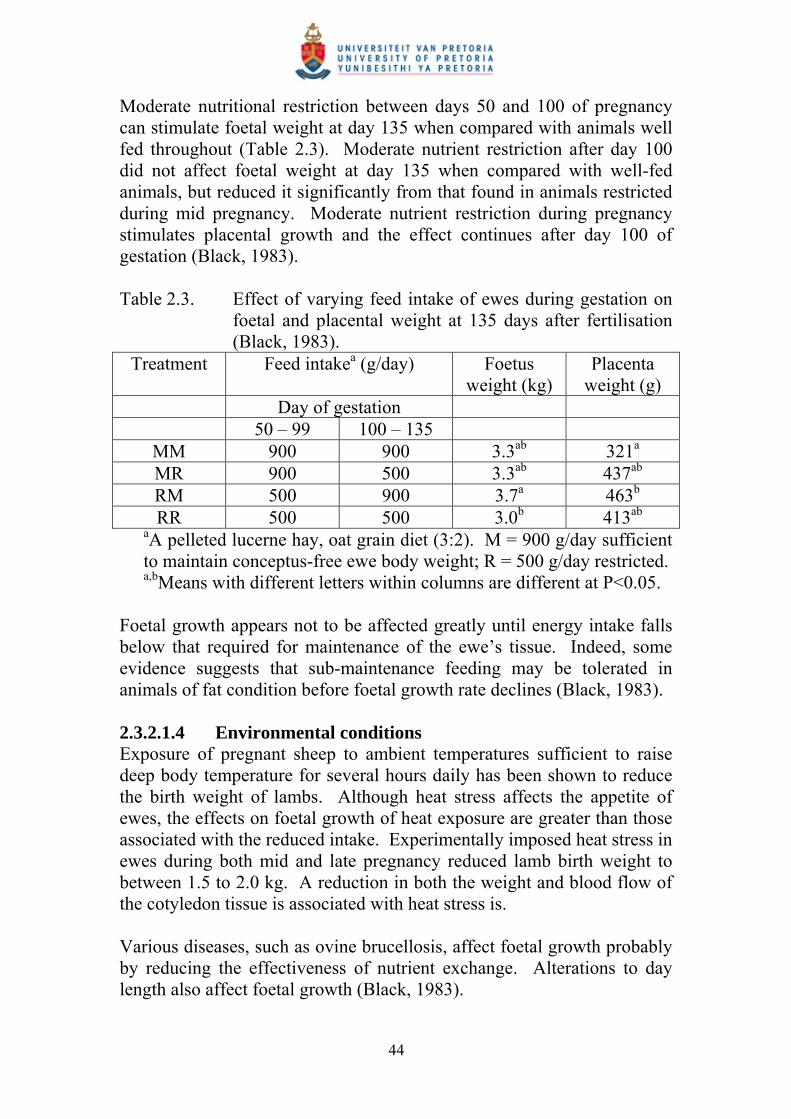
44

Moderate nutritional restriction between days 50 and 100 of pregnancy can stimulate foetal weight at day 135 when compared with animals well fed throughout (Table 2.3). Moderate nutrient restriction after day 100 did not affect foetal weight at day 135 when compared with well-fed animals, but reduced it significantly from that found in animals restricted during mid pregnancy. Moderate nutrient restriction during pregnancy stimulates placental growth and the effect continues after day 100 of gestation (Black, 1983). Table 2.3. Effect of varying feed intake of ewes during gestation on

foetal and placental weight at 135 days after fertilisation (Black, 1983).

Treatment Feed intakea (g/day) Foetus weight (kg)

Placenta weight (g)

Day of gestation 50 – 99 100 – 135

MM 900 900 3.3ab 321a

MR 900 500 3.3ab 437ab

RM 500 900 3.7a 463b

RR 500 500 3.0b 413ab

aA pelleted lucerne hay, oat grain diet (3:2). M = 900 g/day sufficient to maintain conceptus-free ewe body weight; R = 500 g/day restricted. a,bMeans with different letters within columns are different at P<0.05.

Foetal growth appears not to be affected greatly until energy intake falls below that required for maintenance of the ewe’s tissue. Indeed, some evidence suggests that sub-maintenance feeding may be tolerated in animals of fat condition before foetal growth rate declines (Black, 1983). 2.3.2.1.4 Environmental conditions Exposure of pregnant sheep to ambient temperatures sufficient to raise deep body temperature for several hours daily has been shown to reduce the birth weight of lambs. Although heat stress affects the appetite of ewes, the effects on foetal growth of heat exposure are greater than those associated with the reduced intake. Experimentally imposed heat stress in ewes during both mid and late pregnancy reduced lamb birth weight to between 1.5 to 2.0 kg. A reduction in both the weight and blood flow of the cotyledon tissue is associated with heat stress is. Various diseases, such as ovine brucellosis, affect foetal growth probably by reducing the effectiveness of nutrient exchange. Alterations to day length also affect foetal growth (Black, 1983).

45

2.3.2.2 Prediction of foetal growth rate 2.3.2.2.1 Organ development and body composition The increase in live weight of an animal is associated with a marked change in shape and function of various organs. At birth the head and legs are relatively large, but with time the upper muscles of the leg develop and the body becomes proportionately larger. This is the case because different parts in the body grew at different rates thus the pattern of growth varies between tissues (Cooper and Willis, 1989). Relative to the rate of change in foetal weight, some organs such as the liver, thymus, brain and lungs develop rapidly in early gestation and may even fall in weight towards birth. Others, like the adrenals, skeleton, muscles and fat depots tend to develop most rapidly late in gestation. Wool follicles mature mainly between days 90 and 130 of gestation. The differential pattern of organ growth influences the way data should be examined when attempting to determine the consequences of retardation in foetal growth, on the relative development of individual organs (Black, 1983). 2.3.2.3 Consequences of prenatal growth retardation 2.3.2.3.1 Young animal survival The major consequence of prenatal growth retardation is on lamb survival. Compared with normal lambs, low birth weight animals have reduced insulation due to the smaller number of wool fibres, greater relative heat loss because of their larger surface area/unit of body weight, and a reduced capacity to maintain heat production because of their lower fat and energy reserves. All these factors increase their susceptibility to environmental stress and reduce their ability to compete with normal-sized siblings (Black, 1983). 2.3.2.3.2 Growth rate, body composition and ultimate body size Lambs from the well-fed ewes are considerably larger than those from the poorly fed animals; they also appear stronger and more alert (Wallace, 1948a). A reduction in growth rate of lambs has been observed following restricted maternal nutrition during pregnancy (Wallace, 1948b). The plane of nutrition of the ewe markedly affected the weight of the foetus at 144 days during the latter part of pregnancy, while at 91 days the level of the diet had apparently been without effect (Wallace, 1948c). Weight gains of the lambs of ewes on restricted feed suffered a post-natal, as well as a pre-natal nutrition penalty. This was almost certainly due to lower milk production by the ewes poorly fed during gestation (Short, 1955).

46

The effects of nutrition during mid-pregnancy in our experiment were reflected in the lambs’ chance of survival and in their growth rate. A positive relationship exists between the plane of nutrition of the ewe during early to mid-pregnancy and the birth weight and growth rate of the lamb. The survival rate of the lambs was closely related to their birth weight (Curll et al, 1975). It is however, not possible to distinguish the effects of a lower milk production of the ewe from a reduced capacity of the lamb to grow (Black, 1983). As cows grew to about 5 years of age, variances increased, and variability increased most from 2 to 3 years of age (Meyer, 1999). 2.3.2.3.3 Wool growth Growth retardation during late pregnancy can affect wool production of adult sheep from some breeds. Although the number of secondary follicles was reduced by prenatal growth restriction in merinos, a compensatory increase in the growth of each fibre meant that there was no difference in wool production at 200 days of age between lambs from ewes fed differentially during pregnancy (Black, 1983). 2.3.3 Postnatal growth and development During postnatal life, growth rate of the lamb is primarily determined by energy intake relative to live weight. Under ideal conditions, growth rate tends to remain relatively constant from soon after birth until the animal reaches about half mature weight when it then progressively declines to zero at maturity. Rate of growth and the relative development of tissues can be modified by composition of the diet, breed and sex of animal and environmental conditions such as disease and extremes in ambient temperatures (Black, 1983). Changes in weight once mature size has been reached are merely due to the addition of corporal fat and do not constitute true growth. In general terms the termination of growth occurs when production of somatotrophic hormone from the anterior pituitary gland is insufficient to stimulate further growth activity. The amount of somatotrophic hormone increases throughout life, but expressed as the ratio of somatotrophic hormone to body size it declines. Once an animal is mature, there is only sufficient somatotrophic hormone to replace worn and damaged tissues and as a result no further growth occurs. Genetic differences between fast and slow growing animals may reflect their differing ability to produce somatotrophic hormone (Cooper and Willis, 1989).

47

2.3.3.1 Postnatal growth of organs and tissues Differences in the relative growth rate of organs and tissues continue throughout postnatal life. By convention, tissues which are of a greater proportion of the mature weight than body weight, or which increase in weight at a slower relative rate than body weight over the postnatal period are classified as early maturing. Tissues, which have the converse characteristics, are classified as late maturing. In many studies, allometric relationships between tissue weight and body weight have been used to make these classifications. Most internal organs in sheep are early maturing. Brain represents the extreme; having reached about 90% of its maximum size by the time the animal is 35% of mature weight. The small intestine is early maturing, whereas the large intestine and abomasum mature at a rate similar to the whole body. The rumen, reticulum and omasum increase in weight extremely rapidly early in postnatal life, and there is some indication that the total weight of the digestive tract falls as maturity is approached. The orders of maturation of the major body components are skeleton, muscle and fat, with only fat being classified as late maturing (Black, 1983). 2.3.3.2 Factors affecting chemical composition of the whole body 2.3.3.2.1 Age and body weight Physiologically, fattening seems to consist of two major phases. The initial phase is primarily associated with an increase in the number of fat cells; the second physiological phase is concerned solely with cell enlargement and is the fattening phase of growth. A linear model adequately describes the relationship between fat weight and body weight within any phase with fairly abrupt transition from one phase to the other. The duration of the initial phase and the amount of fat present can be influenced by environmental factors, particularly nutrition. Both phases are modified by genetic influences (Searle and Griffiths, 1976). 2.3.3.2.2 Sex and breed When comparisons are made at the same weight, genotypes which are heavier at maturity generally grow faster, contain less fat and more protein and bone in their whole bodies and carcasses than do animals of smaller mature size (Thompson et al, 1979). The sexes do not differ in body-fat content at body weights below the phase change in females (14 kg), that is the fattening phase of growth (Searle and Griffith, 1976).

48

It was observed that the rate of change in body fat with body weight during both the pre-fattening and fattening phases of growth were the same for entire males and females, but the transition to the fattening phase was later in males (Black, 1983). Wethers have more bone and less fat than ewes at the same carcass weight (Thompson et al, 1979), but the differences are smaller than between entire males and females (Black, 1983). According to Robelin and Tulloh (1992) the rate of gain is 10 to 20% higher in bulls than in steers (8% according to Louw (1992)), it is similar in steers and heifers (according to Louw (1992) steers grow 6% faster) and it is 5% higher in heifers than in spayed heifers. Searle and Griffiths (1976) developed the following equation to describe the two-phase relationship between body fat and body weight. Fw = 0 - 2Wp + 1W + 2[(W - Wp) + ]0.5 where Fw is weight of body fat, W is empty body weight, is a curvature parameter, Wp, 0, 1 and 2 are parameters which describe the linear asymptotes such that 0 is the intercept of the asymptote for the first phase, 1 - 2 is the slope of this line, 1 + 2 is the slope of the second phase asymptote and Wp represents the point of transition between the two linear phases. A similar equation can be developed to describe the relationship between body protein and body weight (Black, 1983). Female calves exhibited lower live weight gain and feed conversion rates than bull calves (Toullec, 1992). 2.3.3.2.3 Nutrition Growth may be slowed down or even cease long before the animal reaches mature size. In this instance the limiting factor does not necessarily have to be the somatotrophic hormone concentration, but it may be a shortage of nutrients and the like. In the later stage of an animal’s development, the animal is most frequently limited by its own internal physiology or by dietary aspects (Cooper and Willis, 1989). The effect of level of feeding on sheep was studied. The effects of increasing the intake of a protein adequate diet on the partition of energy in sheep were studied. When the animal is in an energy balance that is at maintenance there is a gain in body protein and a loss of body fat. Further, once energy intake is raised above the level where fat deposition commences, the ratio of the gain in fat to the gain in protein is constant for each increment in energy intake. Consequently, as energy intake is raised above maintenance, the proportion of fat to protein deposited in the

49

body increases exponentially from –1 to an asymptote equivalent to the constant ratio of fat to protein for increments of energy intake above that at which fat is deposited. An increase in the intake of a well balanced diet above maintenance, therefore, results in a faster rate of growth and an increase in the fat content of the gain. However, the effects on body composition are greatest when intake is raised from near maintenance rather than when it is increased above an already high level. An increase in fat content of the energy gain means that animals have more fat when compared at the same weight as animals receiving less energy. The curvilinear relationship between intake of a well-balanced diet and fat deposition can explain why an increase in fat content is sometimes observed, whereas in other experiments there is no effect of increasing the level of feeding; the outcome depends upon the levels of feeding relative to maintenance (Black, 1983). It has been suggested that much of the variation in estimates of the protein requirements of lambs results from failure to differentiate between the total needs of the animal’s tissues for nutrients and the capacity of different diets to provide the tissues with these nutrients. Failure to make this distinction means that most estimates of protein requirements are applicable only to the very limited conditions of the particular experiments from which they were derived. Because the requirement of the tissues for a nutrient in animals of a similar breed, sex and physiological state is relatively constant, and the availability of that nutrient from different diets often highly variable, the tissue requirement for that nutrient must be known before information on its availability can be used in the formulation of diets, or for the prediction of animal performance. When lambs received insufficient protein, the nitrogen balance was independent of metabolisable energy intake and was linearly related to nitrogen absorption. Under conditions of inadequate protein absorption, nitrogen balance was influenced by live weight. The effect of changes in live weight on nitrogen balance was dependent on metabolisable energy intake. Below a certain metabolisable energy intake the rate of mobilisation of body protein is increased (Black and Griffiths, 1975). The composition of body weight loss is influenced by the severity of intake restriction. With intakes near maintenance, there is considerable loss of body fat but little change in body protein. However, when intake is reduced to below half maintenance, the amount of energy lost as protein increases substantially. Thus, when compared with normal

50

growth, animals that are fed near maintenance will tend to be leaner, but those placed on a severely restricted diet will initially be fatter (Black, 1983). Experiments in which the effects of the plane of nutrition on body composition were investigated, suggest that raising energy intake can either increase, have no effect on or decrease the weight of fat in the body or carcass at a particular body weight. The reports showing either a positive, or no effect of increasing energy intake on body fat content, can be explained by the predicted curvilinear relationship between energy intake and fat deposition for diets adequate in protein. This curvilinear relationship has been observed in calves. The experiments show a decrease in body fat with increasing plane of nutrition can be explained by the feeding of low protein diets, or the feeding of diets in which the protein source was extensively degraded within the rumen, and in which case, increasing energy intake would be expected to stimulate protein absorption to a level that would fulfil the animal’s requirements. The feeding of protein deficient diets produces animals with more fat at a given body weight, and the effects become progressively less marked as protein intake approaches requirement (Black, 1974). The initial effect of weight loss and regain was to produce animals with more or less fat respectively than controls of the same empty body weight. Low fat content of weight gain in the early stages of compensatory growth has also been reported for adult sheep. Body water content showed opposite trends to fat content. Since the weight of ash in the body depends on age as well as on weight, it is not surprising that weight loss was not the reverse of growth in the respect of ash (Searle et al, 1979). The absorption of protein in sheep was also studied. As protein absorption increases, the proportion of energy deposited in protein increases until protein availability is no longer limiting. The amount of energy deposited in fat decreases if it is over the same range in protein absorption. Thus, the ratio of fat to protein in the body gain decreases markedly as protein absorption increases from deficient levels. Moderate increases in protein absorption above the animal’s requirements appear to have little further effect on the fat to protein content of the gain (Black, 1983). Lambs that were fed low to high protein levels were more efficient in their utilisation of metabolisable energy for gain than were the high protein controls, especially just after the change of diet. It occurred despite the relatively larger contribution of protein to energy gain of the

51

lambs. Energetic efficiency of protein deposition is inferior to that of fat deposition, both in sheep and pigs. Thus lambs which are fed diets in which protein absorption is below requirement, grow more slowly and contain more fat than animals of the same weight receiving adequate protein (Ørskov et al, 1976). The net efficiency of metabolisable energy utilisation of diets of low protein content is greater than that of diets of high protein content. The energy cost of fat synthesis will vary according to the particular nutrient in major supply and, consequently, to the particular biochemical pathways followed during synthesis. Similarly, the energy cost of protein synthesis will be affected by the quality of the dietary protein, by the concentration of protein in the diet, and by the total amount of protein fed, relative to the energy requirements of the animal. If too little energy is supplied, or an excess of protein is present in the ration, the animal may use protein as a source of energy. This will result in an increased loss of amino groups as urea, and a consequent increase in the energy that must be debited against the weight of protein synthesised (Walker and Norton, 1971). Under these conditions, it is probable that less energy is available for lipogenesis and the ratio of fat to protein in the gain falls below that which occurs in animals given better balanced diets (Black, 1983). The protein and energy interaction in sheep was studied. The decline in protein synthesis that occurs when protein absorption falls below requirement means that the net gain in body protein, seen at energy balance in animals receiving adequate protein, gradually turns into a net loss as protein absorption becomes more inadequate. Animals receiving diets grossly inadequate in protein, gain fat and lose protein when in energy balance. Thus, the effect of increasing feed intake on the ratio of fat to protein in the gain depends upon the adequacy of dietary protein. In contrast to animals fed adequate protein, a severe protein deficiency results in a decline in the ratio of fat to protein in the gain, as feed intake increases. At some intermediate levels of protein intake, there will be no effect of feeding level on body composition (Black, 1983). Refeeding after periods of nutrient restriction results in the growth rate of lambs being normally greater following refeeding after periods of prolonged under nutrition than is observed in animals of the same weight given unlimited access to feed (Black, 1983). The net effect of growth was that economies in energy and nitrogen use were affected while the animals were underfed, but lost when super maintenance feeding was

52

restored. A high voluntary intake was the main feature of compensatory regain (Graham and Searle, 1979). It has been postulated that because there is a decrease in basal metabolic rate with severe underfeeding, and that this sometimes continues into the early refeeding period, it should be possible to find a decreased cost of maintenance in the realimented animals. There is also no difference in maintenance cost during compensatory growth (Drew and Reid, 1975). The effect of a period of live-weight loss was studied on the relationship of selected muscles to total side muscle during subsequent re-alimentation. It was found that the interrupted growth path decreased the proportion of total side muscles formed by the weight of ten muscles, which had previously been classified as muscles with a high growth impetus (Murray and Slezacek, 1975). 2.3.3.2.4 Climatic conditions Adverse environmental conditions are often of greatest importance in early life, whereas in the later stage an animal is most frequently limited by its own internal physiology or by dietary aspects. This is one reason why a product such as an antibiotic (which protects against the environment) is most successful in early life (Cooper and Willis, 1989). Conditions that require the animal to produce extra heat to prevent hypothermia are better understood. It is assumed that ‘cold stress’ does not affect nitrogen metabolism, but the evidence on sheep is insubstantial and the more extensive data on pigs is equivocal. Below a certain ambient temperature (the lower critical temperature), heat production rises as temperature falls, and level of feeding has a relatively small effect (heat increment is approximately 20% of metabolisable energy). Normal heat production is first determined as metabolisable energy less energy balance in tissues and all products. Metabolisable energy requirements for maintenance is also incremented by an amount equal to the additional heat production due to cold stress (Graham et al, 1976). Moderate cold stress does not affect protein deposition but reduces growth rate and fat synthesis. Although the rate of protein synthesis can be depressed in animals subjected to cold stress, this occurs only when conditions are so severe that survival is threatened (Black, 1983). Estimates of temporary, environmental variances were highest for 3-year-old cows, resulting in lowest estimates of heritabilities and repeatabilities for this age. For later ages, estimates of these parameters were consistently higher than from repeatability model analysis, indicating that

53

we can discriminate better between animal and extrageneous effects when accounting correctly for differences in variability at different ages (Meyer, 1999). 2.3.4 Conclusion Foetal growth is determined primarily by the rate of nutrient exchange across the utero-placenta. It is influenced by the sex and genotype of the foetus, litter size, body weight and condition of the ewe, maternal nutrition during mid and late pregnancy and environmental factors such as high ambient temperature and disease. Small deviations in tissue development result from severe foetal growth retardation, such that small lambs at birth tend to have lighter livers, less fat and fewer wool follicles but larger skeletons relative to their weight than do normal foetuses. During the postnatal period, growth rate and the relative distribution of fat and lean within the body are affected by the sex, breed and stage of maturity of the lamb, as well as by energy intake, composition of the diet and climatic conditions. Within each genotype, there appears to be a maximum rate of energy deposition with the partition between protein and fat varying with body weight. There is no simple relationship between growth rate and body composition of sheep. However, from an understanding of the partition of absorbed nutrients between various body functions, it is possible to explain the association between these characteristics in specific situations (Black, 1983).

54

CHAPTER 3

GROWTH CURVE MODELLING AND DATA 3.1 Introduction Since growth is essentially a quantitative phenomenon the rate is the most important property. If the multiplicative rate of growth were constant, the graph of size or mass against time would be exponential (Needham, 1964). Growth in body weight in relation to time can be described as sigmoid under normal circumstances (Fowler, 1980); a roughly S-shaped curve (Hammond, 1955), which is a characteristic curve (Du Preez et al, 1992). The growth curve is much the same shape for all species (Brody, 1945). Most animal species have a typical growth curve that is sigmoid or S-shaped, involving a relatively slow period in early life, a self-accelerating phase and finally a self-inhibiting phase when growth again slows down and finally ceases (Cooper and Willis, 1989). The interaction of two opposing forces, a growth accelerating force and a growth retarding force, produces the general shape of the growth curve (Brody, 1945). When the slope of the growth curve is increasing, the growth accelerating force is predominating and when the slope of the growth curve is diminishing, the growth retarding force is predominating. The growth accelerating force arises from the nature of growth in weight; this is a summation of cell multiplication, cell hypertrophy and the inclusion of material taken from the environment (Hammond, 1955). In the absence of inhibiting factors, living cells are capable of growing for an indefinite period. The individual cells tend to reproduce at a constant rate so that the growth of the mass of cells representing the whole organism tends to be self-accelerating (Brody, 1945). For this reason the part of the growth curve during which the growth accelerating force is dominant, is sometimes referred to as the ‘self-accelerating phase of growth’. Within the closed system represented by the animal body, there comes a stage in growth when further growth tends to be limited by growth inhibiting factors such as availability of nutrients and lack of space. From this point growth is limited by the growth retarding force, and this part of the growth curve is consequently referred to as the ‘self-retarding phase of growth’ (Hammond, 1955). Ultimately growth is completely inhibited by the environment and this is followed by senescence and finally by death (Brody, 1945).

55

Where the two segments of the growth curve represented by the self-accelerating and self-retarding phases of growth intersect, is the point of inflection. This point of inflection represents the point in the growth curve when the acceleration of growth has ended and the retarding of growth is about to begin, and it is therefore the point at which growth rate is at a maximum (Hammond, 1955). The point of intersect (or inflection point) are joined during puberty in animals, flowering in plants and ‘coming of age’ in populations of organisms (Brody, 1945). A growth curve, that is graphs of size/time, in fact often are exponential under ideal conditions, as in the early stages of growth in most organisms, and indefinitely in microorganisms under special experimental conditions. The curve is one of increasing steepness, which is indicated by the equation to its slope, dx/dt, where x is the size and t is time. This is also the gross growth rate, so that total size increases with continuous acceleration (Needham, 1964). 3.2 Definitions of growth rates The aim of a growth model is to integrate existing knowledge allowing the prediction of growth rate, but also to indicate possible axes of research where knowledge is limited. The classical and well documented approach was to relate animal weight to time through empirical equations describing growth curves (Bastianelli and Sauvant, 1997). Growth models summarise information needed to understand the biological phenomenon of growth, which is an important component in beef production systems. Development of a growth model that describes the growth pattern of a herd, within a particular environment and management system, may be useful to determine the relative importance of factors affecting production efficiency (Menchaca et al, 1996). For purposes of quantitative analysis, growth may be defined as relatively irreversible time change in magnitude of the measured dimension or function. The concept of irreversibility is emphasised to exclude fluctuating time changes of a fortuitous nature, such as those occasioned by fluctuating food supply with consequent fattening and leaning, with gestation, lactation, and so on. Growth in weight is usually represented in one or all of the three ways: (1) absolute gain in the given magnitude per unit time; (2) relative rate (or percentage when multiplied by 100) gain per unit time; (3) cumulative, or course-of-growth weight up to, or the weight at, a given time. All these

56

forms of representation may be made in conventional mathematical terminology (Brody, 1945). 3.3 Choice of appropriate model Each component of an organism – whether cell, tissue, organ or whole body – follows an inherent growth pattern influenced by the environment in which pattern is expressed. Thus, at any given time of observation, the growth curve for a trait, such as body weight, will represent the composite of growth curves for all the components contributing to the trait. A fitted size-age relationship suitable for one component may be inappropriate for another component or composite trait. However, such ‘rule of thumb’ generalisations about the relationships between different measures of size can be misleading. Allometric analysis of relative growth rates for different measures of size have shown that such relationships vary for different traits, for different genotypes and for different phases of growth (Fitzhugh, 1976). Traditionally, selection in beef cattle has emphasised heavy weights at market ages. For the cattle feeder, this criterion is associated with faster growth rates and increased economic returns over short periods of time. However, high growth rates to market age may also result in larger mature weights of breeding cows and, as a consequence, increased maintenance costs. Larger cows of synthetic lines have been found to be less efficient in reproduction and cow productivity than smaller cows under similar management systems. The precision in estimating mature weight, however, can be seriously affected by temporal environmental variation. The accuracy of the equations for estimating mature weight and maturing rate need to be improved, which implies adjustment for early reproduction and other environmental factors, and the inclusion of some measurement of skeletal size, such as hip height (Beltrán et al, 1992). A common characteristic of growth models to be discussed is that they each utilise (directly or indirectly) two biologically relevant parameters. The first parameter establishes the position of the individual (or group) in the general size space at a given reference age, usually maturity. In other words, the size parameter establishes whether the individual is large, medium or small (Fitzhugh, 1976). Two factors that affect cow weights are age and lactation stress (Morrow et al, 1978). Correlations among different measures of size, for the same individual at the same (or different) ages tend to be quite high. Thus the size parameter may be

57

taken as generally indicative of body size, an exceedingly important trait given the reported relationships of size to a diverse range of traits, including litter size, dystocia, growth rate, milk production, maintenance requirements, optimal slaughter weights and economic efficiency. The second parameter is concerned with growth rate relative to body size. When the size parameter refers to mature size, this ‘rate’ parameter defines average maturing time, which has been related to intrinsic efficiency of growth. In addition to the size and rate parameters, a third parameter is often used to partition the growth curve into stages, which is called ‘self accelerating’ and ‘self inhibiting’ stages during which growth rate velocity is increasing and decreasing, respectively. Transition between these two stages establishes the point of inflection of the sigmoid growth curve, thus this third parameter will be referred to as the inflection parameter. Since the growth curve is essentially linear during the interval when this transition theoretically occurs (e.g., for cattle, the age interval 6 to 18 months), the estimated point of inflection may be influenced less by the animal’s phenotype and more by the properties of the specific equation chosen to fit the data (Fitzhugh, 1976). 3.4 Variation Biological variation differs from that observed in many other fields in such a way that it is often due largely to substantive factors (genetical, physiological, environmental, etc.), and only in small part to errors or inaccuracies. Consequently, the extent of individual variation in growth curves within biological populations is of considerable interest in itself. Tolerance limits and prediction limits (confidence limits for a new individual observation drawn from the same population as the sample in hand) confound the uncertainty of sample estimates with the estimated extent of individual variation and do not provide a satisfactory description of the latter, even though they are currently used for this purpose. Many kinds of biological varieties, such as somatic dimensions or numbers of individuals in animal, plant or bacterial populations, have positively skewed heteroscedastic frequency distributions and cannot assume negative numerical values. In principle, when one attempts to describe the growth of such a variant x with respect to time t, one would thus expect satisfactory results from a multiplicative error model, possibly involving the lognormal distribution:

Xi = f ( A, B, C, …; t ) σ ei

58

where f ( A, B, C, …; t ) is a null- or positive-valued deterministic linear or non-linear function of time, involving parameters A, B, C, …; σ is the residual standard deviation of observations Xi about the function f ( A, B, C, …; t ) on the natural logarithmic scale; and ei is a standardised random normal deviate. In practice, it comes therefore as a surprise that growth data are often fitted better by an additive error model:

Xi = f ( A, B, C, …; t ) + σei than by a multiplicative model (Jolicoeur and Heusner, 1986). 3.5 Non-linear models The model provides a mathematical framework to investigate possible sampling patterns for optimal allocation of resources. The simulations show that it can satisfactory estimate average growth curves with limited information (Palmer et al, 1991). The fitting of mathematical models to longitudinal growth data is a widely accepted method of summarising the information on an individual. Also, growth velocities and accelerations are easily estimated from fitted models (Berkey, 1982). 3.6 Measures of growth The most common measure of growth is probably an increase in live weight, but frequently various measures of size such as height and length are also used. A combination of live weight and measures of size is frequently more informative than live weight alone, because it records the changes in shape that occur during normal growth and demonstrates that an animal may continue to increase in size even though the body weight is kept constant (Hammond, 1955). Most conclusions about the growth of cattle tend to be based on observations made only on females. Where males have been considered, information pertains mostly to castrates (Doren and Baker, 1989). Improving the bioenergetics efficiency of body-weight growth in cattle depends on understanding how genetic and environmental factors can be used to manipulate attributes such as average lifetime rates of growth, and maturing independently of mature weight, thus altering the shape of the growth curve (Perotto et al, 1992). The mean estimates of the growth constants for several breed groups (Table 3.1) were used as a basis for examining models. The different

59

breed groups provided rather large differences in growth patterns from which to examine the flexibility of the models. The parameter for asymptotic weight offered the best opportunity to make direct comparisons among all models, since the other parameters measure slightly different phenomena. The different models are:

1. Von Bertalanffy 2. Brody 3. Gompertz 4. Richards

Algebraic models provide an effective method of reducing the number of descriptive parameters needed to describe individual growth patterns. Such models tend to average out the effects of temporary environment, as well as to adjust for the non-linear effect of age on weight. If the selected model accurately describes the data and closely approximates the underlying biological functions, the research scientist may choose to investigate the properties of the empirical model in much the same manner as he would investigate the true biological model were it known. The selection of any one of the proposed models, or some modified form of these models, depends upon the nature of the study and the intended application of the results (Brown et al, 1976). Table 3.1. Estimated parameters for five-growth models’ least

squares breed group means (Brown et al, 1976). Von Bertalanffy Brody Gompertz

Logistic Richards

Breed

groupa

No. obs. A

c Bc K

c A

c BA

c K

c A

c Y0

c L

c A

c K

c M

c A

c B

c K

c M

c

H 11 488 0.50 0.065 508 487 0.049 498 75 0.140 0.070 481 0.083 2.53 505 0.79 0.052 2.33

1B1H 27 533 0.52 0.076 543 532 0.057 5 4 1 78 0.179 0.084 524 0.096 2.68 549 0.83 0.088 1.74

3H1B 25 515 0.55 0.087 542 536 0.060 506 66 0.226 0.104 496 0.116 2.84 533 0.74 0.088 3.08

5H3B 17 515 0.60 0.105 499 516 0.073 474 52 0.272 0.118 467 0.134 2.97 494 0.87 0.097 2.26

AX 11 444 0.65 0.117 471 504 0.076 438 35 0.375 0.137 434 0.152 3.48 477 0.77 0.110 3.32 Beef breed

average 91 499 0.56 0.090 513 515 0.063 491 61 0.238 0.103 480 0.116 2.90 509 0.80 0.087 2.55

Jersey 147 416 0.56 0.064 454 449 0.044 414 44 0.166 0.074 401 0.086 3.01 424 0.70 0.058 2.94 aH = Hereford; B = Brahman; BH = combinations designate proportion of B and H in the respective crosses; AX = Angus x BH crosses; Beef breed average = the pooled breed groups at the East Texas Pasture Laboratory, Lufkin (where this study took place). cA, B, K, L and M are fitted parameters; Y0 = weight when t = 0; A, BA and Y0 measured in kilograms; other parameters are unit less. Rate of growth (Brody, 1945) in weight may be expressed as average growth rate, that is as absolute gain in weight per unit time, expressed by the formula:

60

W2 – W1

t2 – t1 where W2 – W1 is the gain in weight during the time interval t2 – t1. This average growth rate is frequently used in animal experiments when the results of the experiment are summarised by saying that, for example, during the experimental period, treated animals gained x grams per day whereas the control animals only gained y grams per day. The average growth rate expressed in this way is open to very small objection providing that the interval t2 – t1 is short. If t2 – t1 is long, the average growth rate gives no idea of the growth rate at any particular time. An alternative method of expressing growth rate is by means of the relative growth rate, that is, the weight gained in a given time expressed in relation to the weight at the beginning of that time. Relative growth rate (Brody, 1945) is expressed by the formula:

W2 – W1

W1 where W1 is the initial weight and W2 is the final weight. For convenience, relative growth rate is usually expressed as a percentage and is useful for comparing growth in different species of widely different body weights. Again the formula for relative growth rate can be misleading if the gain in weight is very large in comparison with the initial weight. Under these conditions the relative growth rate gives no idea of the growth rate at the time when the final weight was recorded. The ‘instantaneous growth rate’ (Brody, 1945) could also be used. This growth rate is obtained by dividing the instantaneous weight gain dW/dt by the W which is the weight at which dW/dt is measured. Instantaneous relative growth rate is expressed by the formula:

k = dW W

/dt

where k is the instantaneous relative growth rate. This is useless for practical purposes because of the impossibility of measuring the instantaneous weight gain dW/dt so the formula is written in the integrated form:

W = A e k t

61

Where e is the base of natural logarithms and A is the natural logarithm of W when t = 0. This formula is applicable to the self-accelerating phase of growth when the relative growth rate is a function of growth already made. During the self-inhibiting phase of the growth curve, the relative growth rate is a function, not of growth already made, but of growth yet to be made to reach maturity (Hammond, 1955). A much-used equation for postnatal growth is:

W = A ( 1 – e – k ( t – t*) ) where A is mature weight; W is weight at age t; t* is the time origin of the curve; and k is an index of the decay of the curve with time. The equation has no inflection and relates to that part of the growth curve that is self-decelerating. To apply it strictly to the growing animal is not entirely appropriate, since the growth of an animal is linear over a considerable period. It is, however, a comparatively simple equation in which the constants have a clear biological meaning (Fowler, 1980). The normal curve of growth of beef cattle can be described in quantitative terms by means of the Gompertz equation (Prescott, 1976):

W1 = W0e α

A ( 1 – e – t1)

or the Gompertz equation (García-Muñiz et al, 1998) for lifetime live weight-age can be as follows:

W1 = Ae – be-kt

where W1 is live weight at age t1. W0 is initial weight at age t

0, which may

be taken to be either soon after conception or at birth. e is the base of the natural logarithm. A is the initial specific growth rate at t

1. α is the rate

of exponential decline of the specific growth rate. A, b and k are

parameters to be estimated. A is asymptotic value for live weight as t∞ ,

generally interpreted as average mature weight. This equation has been used to describe both the prenatal and post-natal growth of mammals (Prescott, 1976; García-Muñiz et al, 1998).

62

Mature weight is a highly inheritable trait according to Kaps et al (1999). This means that mature weight can be altered by selection. If mature weight breeding values are predicted from a genetic evaluation, mature weight should be jointly analysed with some other trait measured earlier in life to account, at least partly, for any effect of culling. Implications for a selection programme would be similar regardless of whether breeding values were estimated from repeated measures, mature weight or mature weight predicted from the non-linear growth functions (Kaps et al, 1999). 3.7 Analysis of growth data Growth defined by curves has definite advantages over age-weight points. In order to describe lifetime growth, unique traits must be defined, and growth curves provide parameters that can describe lifetime growth biologically. Weights predicted from growth curves have advantages over single age-weight points. A single weight is a point in time, dependent on the quality and quantity of feed, seasonal affects and random environmental effects. The curve-fitting procedure smoothes those deviations by using previous and future weights to predict a specific age-weight point. In fact, each single age-weight point predicted from a curve is actually adjusted for individual environmental effects that cannot be removed from an analysis of actual age-weight points. On the other hand, weights recorded over time contain correlated errors that cannot be removed from a longitudinal study (Denise and Brinks, 1985). Longitudinal data is a complete set of measurements that is available for every individual at every age (stage). Longitudinal data includes all information available in static and cross-sectional data, plus information on individual variation in growth. Even when longitudinal data is partitioned into subsets for cross-sectional or static analysis, confidence in the interpretation is increased since the same individuals contribute to all levels of the analysis. An information-rich continuum of size-age points is a challenging analytical problem. First, the objectives for the analysis must be clearly established. Primary objectives for fitting growth curves are descriptive and predictive: Descriptive information contained in the sequence of size-age points is consolidated into relatively few parameters, predictive growth curve parameters are utilised either separately or in concert to predict growth rates, feed requirements, responses to selection and other items of interest (Fitzhugh, 1976).

63

Year of birth was also an important source of variation for the b (P<0.01), k (P<0.05) and m (P<0.01) parameters of Richardts’ function. Mating system was an important source of variation for the A parameter of Brody’s and Richardts’ function (P<0.01) (Denise and Brinks, 1985). Special characteristics of the data set and objectives of analysis determine the method of choice for fitting the growth curve. Primary basis for comparing methods of fitting growth curves include:

· Biological interpretability of parameters generally depends on understanding the interrelationships of genetics and the environment that yielded a particular pattern (phenotype). Care should be taken not to force a biological interpretation, or to casually apply interpretations found appropriate for one set of data to another. Biological interpretability includes ability to correctly rank individuals or populations for important biological characteristics, as might be required in selection programs for growth rate, maturing rate or mature size.

· Goodness of fit to actual data refers to minimising the deviations of actual data points from corresponding points on the fitted curve. In this respect, the best fit to n size-age points is a (n – 1) polynomial, but a (n – 1) polynomial has not consolidated information, nor are the (n – 1) estimated parameters likely to be biologically interpretable.

· Computational difficulty varies with choice of function and the characteristics of a specific data set. Most functions are sensitive to the frequency and regularity of data on both the size and age scales. Algorithms involving iteration are sensitive to choice of starting values, and may not even converge to a solution. Mathematically correct, but biologically infeasible, estimates of parameters may be computed (Fitzhugh, 1976).

3.8 Regression of size on age Equations or functions that regress size on age are obvious choices for fitting size-age data. However, the presumption of a causal relationship between age and size can be misleading. Age per se does not cause size to increase and then plateau, but provides opportunity for the individual’s inherent potential for growth and maturation to interact with particular environments. Cumulative nutrient consumption is an alternative independent variable in place of age (cumulative time). This reference base would dampen fluctuations in size, especially weight, which result from temporary changes in quantity or quality of feed due to seasonal

64

changes or from the changes in requirements associated with level of productivity. A plot of weight against cumulative ad libitum food consumption generally follows an exponential curve (Fitzhugh, 1976). 3.9 Goodness-of-fit characteristics of the growth curves. Several characteristics of the curve-fitting process were calculated for each animal. The sums of squared deviations (SS) of actual and predicted weights were calculated to indicate the overall curve fit. Standard deviations of each parameter were also calculated for each animal to indicate the amount of variation associated with the fit of each parameter. Inbred cows had smaller SS than line crosses. When the weight of an animal was studied throughout the lifetime of the animal, it was found that line cross cows lost more weight under a poor environment and gained more weight under a good environment. This fluctuation in weight between time periods could have directly affected SS. Year of birth was a significant source of variation for SS in both functions. Sires within line-of-sire was also an important source of variation in growth curves (P<0.01). The curves were more appropriate for cows by certain sires, or cows by such sires fluctuated in body weight between weigh periods more than other sire groups. The age covariate was an important source of variation for SS from the curves. Older cows, with more weights, had larger sums of squared deviations because SS were unadjusted for the number of weights.

65

Table 3.2. Parameter estimates and standard errors for growth curves from birth to weaning for Brahman calves of three frame sizes (Menchaca et al, 1996).

Small frame Medium frame Large frame Item Constant SE Constant SE Constant SE

Growth curvea a 3.39282 0.00836 3.48342 0.01228 3.59697 0.00786 A (29.7)b (32.6) (36.5) b 0.463311 0.005915 0.467238 0.007947 0.452262 0.005235c -

0.0264330 0.000800

6 -

0.02785910.001100

8 -

0.0264639 0.000734

0 Sex

Male 0.0447638 0.0064664

0.0295028 0.0122803

0.0367449 0.0062432

(1.04578) (1.02994) (1.03743) Female -

0.0447638 0.006466

4 -

0.02950280.012280

3 -

0.0367449 0.006243

2 (0.95622) (0.97093) (0.96392)

aAge t in months. b( ) = values in the original scale, kg. A = a constant that occurs with every observation. b = growth curve parameters on age t (month). c = growth curve parameters on age t (month).

The standard deviation of the A parameter from Brody’s function was affected by the age-of-dam of the cow and by the sire within line (P<0.05). Cows out of dams 11 years and older had the greatest variation in A. Sire differences in asymptotic weight may be the major contributor to sire differences in sum of squared deviations of Brody’s curve. The standard deviation of the A parameter from Richards’ function was unaffected by any factors in the model. The standard deviations of the b parameters from Brody (P<0.01) and Richards’ (P<0.05) functions were affected by the cow’s year of birth. The standard deviations of the k parameters from both functions were also affected by cow’s year of birth (P<0.01). The m parameter of Richards’ function was unaffected by the factors studied. In comparing the two functions (the Richards’ function and the Brody’s curve), both curves were affected by the same factors. Richards’ function however, had a smaller sum of squares than Brody’s curve. The inclusion of the m parameter in Richards’ function allowed a better overall fit to the

66

actual data points. Brody’s curve required an average of 1.48 fewer iterations for convergence than Richards’ function; therefore, Brody’s parameter had smaller associated standard deviations than Richards’ function. It was found that Brody’s curve was computationally easier to fit than Richards’ function, although Richards’ function fit the age-weight data better than Brody’s curve (DeNise and Brinks, 1985). In Prescott (1976) it was shown that the Gompertz equation provided a consistently good fit to observations on the growth of individual cows. It was also used to describe the growth curves of a selection of Brahman-Hereford crosses, as well as growth curves for ostriches (Du Preez et al, 1992). Estimating mature size in cows using a two parameter Gompertz curve gave a measure with higher heritabilities, and estimates of genetic correlations with early growth than simply using repeated records for adult weights (Prescott, 1976). However for the average mature weight maintained, at least one weight taken at about 4 years of age seemed to be required to obtain reliable estimates (Meyer, 1995). 3.10 Growth patterns Breed type affected all weights and condition scores from birth to 20 months of age. Results of linear contrasts indicated that crossbred females weighed 5.5, 14, 26 and 39 kg more than straight-bred Angus females at birth, weaning, 13 months of age and 20 months of age, respectively. Condition scores of crossbred females averaged lower than those of Angus females to 20 months of age, but Angus and Charolais × Angus females were similar in condition at weaning and 13 months of age (Nadarajah et al, 1984).

67

Table 3.3. Least-squares means and standard errors for heifer weights (kg) and condition scores to 20 months of age (Nadarajah et al, 1984).

Weaning 13 months old 20 months old Breed typea

Birth weight

Weight Condition Weight Condition Weight Condition

AA 28.5 0.5

199 2.5

9.1 0.1

268 3.1

8.0 0.1

356 5.9

9.6 0.2

CC 40.2 0.7

248 4.2

8.3 0.2

339 6.2

8.2 0.2

406 7.4

7.7 0.3

CA 34.1 0.7

216 3.7

9.2 0.2

297 4.0

8.2 0.1

399 7.2

9.2 0.3

FA 34.0 0.7

209 3.8

7.5 0.2

293 4.4

6.9 0.2

391 7.1

7.9 0.3

Contrasts AA vs XBR

-5.5** -14** 0.74** -26** 0.48** -39** 1.63**

CA vs FA

0.05 6.4 1.7** 4 1.3** 8 1.2**

CA vs CC

-6.1** -32** 0.9** -42** 0.01 -7 1.5**

CA vs SBR

-0.58 -7.1 0.5* -7 0.1 18* 0.55 aAA = Angus; CC = Charolais; CA = Charolais × Angus; FA = Holstein × Angus; XBR = crossbreds; SBR = straight breds. *P < 0.05. **P < 0.01.

Charolais females were heaviest at all ages (Table 3.3) but did not differ significantly from Charolais × Angus females at 20 months of age. There was also no significant difference in weight among crossbred types up to 20 months of age, but Charolais × Angus heifers were estimated to be fatter than Holstein × Angus heifers. Weights (except for birth weight) and condition scores were affected by year-to-year fluctuations, and significant breed type × year interactions, suggested that the changing environment affected different types somewhat differently. This interaction may also have reflected random differences among sets of sires sampled from the various breeds in different years. When effects of breed type were tested with the more conservative interaction mean square, breed differences remained significant for weight at all ages except 20 months of age and for condition at all ages. Age of dam did

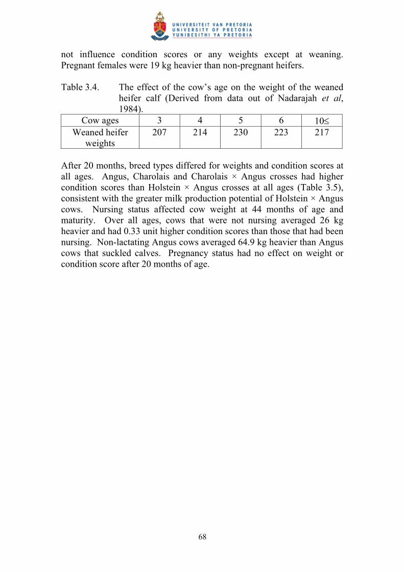
68

not influence condition scores or any weights except at weaning. Pregnant females were 19 kg heavier than non-pregnant heifers. Table 3.4. The effect of the cow’s age on the weight of the weaned

heifer calf (Derived from data out of Nadarajah et al, 1984).

Cow ages 3 4 5 6 10 Weaned heifer

weights 207 214 230 223 217

After 20 months, breed types differed for weights and condition scores at all ages. Angus, Charolais and Charolais × Angus crosses had higher condition scores than Holstein × Angus crosses at all ages (Table 3.5), consistent with the greater milk production potential of Holstein × Angus cows. Nursing status affected cow weight at 44 months of age and maturity. Over all ages, cows that were not nursing averaged 26 kg heavier and had 0.33 unit higher condition scores than those that had been nursing. Non-lactating Angus cows averaged 64.9 kg heavier than Angus cows that suckled calves. Pregnancy status had no effect on weight or condition score after 20 months of age.

69

Table 3.5. Least squares means and standard errors for cow weights (kg) and condition scores from 32 months of age to maturity (Nadarajah et al, 1984).

32 months

old

44 months

old

56 months

old

68 months

old Maturity

Breed type

Weight Condition Weight Condition Weight Condition Weight Condition Weight Condition

AA 348 11.1

2.9 0.13

441 18.7

3.1 0.14

461 15.5

3.5 0.18

466 14.7

3.4 0.18

469 12.2

3.4 0.13

CC 509 12.8

2.8 0.15

578 15.6

2.95 0.18

600 19.0

3.1 0.2

652 33.0

3.6 0.4

580 26.3

3.2 0.3

CA 427 15.5

2.7 0.18

516 14.8

3.2 0.17

506 16.9

2.9 0.2

519 19.0

3.1 0.23

534 13.3

3.1 0.14

FA 410 14.9

2.1 0.18

488 15.6

2.7 0.18

474 16.5

2.4 0.2

490 15.5

2.8 0.18

508 12.6

2.9 0.14

Contrasts AA vs

XBR

-34** 0.54** -62** 0.12 -29** 0.84* -38** 0.46** -53** 0.36*

CA vs FA

17 0.6** 28* 0.45** 32* 0.42* 29 0.32 26 0.21

CA vs CC

-82** 0.1 -62** 0.2 -94** 0.2 -133** 0.5 46 0.04

CA vs SBR

-19 0.2 6 0.2 -25 -0.4* -38 0.4 10 0.30

aAA = Angus; CC = Charolais; CA = Charolais × Angus; FA = Holstein × Angus; XBR = crossbreds; SBR = straight breds. *P < 0.05. **P < 0.01.

Yearly fluctuations had a significant effect on cow weight at 32 and 56 months of age, and at maturity and on condition score at 56 months of age and maturity. Likewise, breed type year interaction was significant for weight at all ages except maturity. The breed type year interaction may be due to individual sire differences or to differential breed responses to yearly fluctuations in feed supply. Angus breed fattened faster and matured earlier than the larger Charolais breed. Weights of Angus cows increased less after 56 months than did those of the other breeds. The Charolais Angus crosses were intermediate in weight to the two straight breeds.

70

The maximum growth of Angus and Hereford females were reported between 5 and 9 years of age. But Angus cows continued to increase in weight up to 8 years of age. The 10 and 11-year-old cows had the higher condition scores. Table 3.6. Least-squares means for cow weights (kg) unadjusted and

adjusted for conditiona, b (Nadarajah et al, 1984). Weights unadjusted for

condition Weights adjusted for

condition Age

(months) AA CC CA FA AA CC CA FA

0 (birth) 30 39 35 35 30 39 35 35 7 200 244 219 215 191 241 221 206 13 272 337 303 297 273 339 310 301 20 360 399 401 397 344 405 403 387 32 398 509 445 426 390 519 467 450 44 427 572 485 466 424 566 490 480 56 438 574 498 474 436 581 503 505 68 459 600 516 492 436 593 507 512 84

(maturity) 459 603 510 503 392 599 527 519

aCalculated from the model Ⅲ analysis. bAA = Angus; CC = Charolais; CA = Charolais Angus; FA = Holstein Angus.

Brody’s model (Table 3.7) (Nadarajah et al, 1984; Doren and Baker, 1989; García-Muñiz et al, 1998; McCurley et al, 1980) is:

Yit = Ai ( 1 – Bie-Kit ) + rit

where Yit is the observed body weight of the ith breed type at time t; Ai is the asymptotic weight of the ith breed type; Bi is 1 minus the ratio of birth weight to mature weight for the ith breed type, thus at t = 0, Ŷit = Ai ( 1 – Bi ); e is the base of natural logarithms ( 2.30259); Ki is the maturing rate of the ith breed type, where rate of gain ( dY/dt ) at time t may be defined as dY/dt = Ki (Ai - Yit), thus the rate of gain is directly proportioned to Ki for types having the same asymptotic weight. Kaps et al, (1999), stated that K1 is a curve parameter representing the ratio of maximum growth rate to mature size referred to as the maturing rate index. Mature rate index is related to the postnatal rate of maturing and serves both, as a measure of rate of change in growth rate and of growth rate; and rit is the

71

mean deviation of the observed weight from the predicted weight for the ith breed group at time t. Richards model (Table 3.7) may be presented (Nadarajah et al, 1984; Doren and Baker, 1998) as:

Yit = Ai ( 1 Bie-Kit )M + rit

where Yit is the observed body weight of the ith breed type at time t; Ai is the asymptotic weight of the ith breed type; Bi is 1 minus the ratio of birth weight to mature weight for the ith breed type; such that at t = 0, Ŷit = Ai ( 1 – Bi ); e is the base of natural logarithms ( 2.30259); Ki is the maturing rate of the ith breed type, where rate of gain ( dY/dt ) at time t may be defined as dY/dt = Ki (Ai - Yit) such that rate of gain is directly proportioned to Ki for types having the same asymptotic weight; rit is the mean deviation of the observed weight from the predicted weight for the ith breed group at time t; and M defines degree of maturity (fraction of A achieved) at the inflection point of the growth curve (ui) as ui = [( M – 1)/ M]M. Table 3.7. Growth curve parameters by cow breed type based on

Brody and Richards’ growth models (Nadarajah et al, 1984).

Brody parameters Richards parameters Breed typea

A B K A B K M

Unadjusted weights AA 453 0.93 0.070 475 0.96 0.061 0.834 CC 608 0.92 0.055 619 0.96 0.045 0.788 CA 511 0.93 0.068 513 0.94 0.065 0.929 FA 491 0.92 0.070 494 0.95 0.064 0.877

Weights adjusted for condition AA 426 0.93 0.077 424 0.85 0.092 1.381 CC 604 0.93 0.058 609 0.96 0.052 0.865 CA 517 0.93 0.063 518 0.94 0.063 0.990 FA 517 0.94 0.069 516 0.92 0.073 1.079

aAA = Angus; CC = Charolais; CA = Charolais Angus; FA = Holstein Angus

3.10.1 Growth phases Growth occurs in different phases. Changes in the growth curve of animals were shown to coincide with certain physiological changes. The

72

genetic correlation between body masses at different ages over the whole growth period is generally positive. It seemed that growth from birth up to 50 kg live mass in sheep, occurred in different phases. Genetic variation exists for growth in these phases. The genetic correlations between growth rates in the different phases of the growth curve were generally positive but not significant. Discrepancies, especially in respect of feed conversion ratio, exist (Greeff et al, 1993). Sire breed, year within sire breed, and sire within year within sire breed affected (P<0.01) all pre- and post weaning growth traits. Dam age affected (P<0.01) all growth traits, except average daily growth from 400 to 450 days of age. Preweaning growth and weight at 400 days of age increased as cow age increased. Average daily gain from weaning to 400 days of age decreased as dam age increased, indicating compensatory post weaning gain for heifer calves from younger cows. Dam breed influenced (P<0.01) all growth traits, except average daily gain from weaning to 400 days of age (Laster et al, 1976). 3.11 Conclusion Decision support is an approach to modelling used to evaluate alternatives and to arrive at decisions. This approach recognises that the owner of the problem is responsible for decisions, and that modelling is used to assist with computation (Gillard and Monypenny, 1987). Using the data from the literature on growth, it is possible to create tables on growth of livestock. This data provides the means through which weight gain can be predicted for livestock. Add to this the water intake of livestock, condition scores at different ages of livestock, the dry matter intake of livestock, the dressing percentages of carcasses of livestock, the average producer prices, the herd composition and mortality rates of livestock and you have all the building blocks for the development of a mathematical model.

73

CHAPTER 4

MATERIALS AND METHODS

4.1 Objectives of the system Mechanistic modelling can be a useful tool in quantitative synthesis and structuring of dispersed information or knowledge, and it can allow the testing of hypotheses on how a system works. Several other objectives can be found for mechanistic models: help in planning experiments, teaching and exploration of alternative farm management strategies. Growth models are generally dynamic because they follow growth through time. By contrast, models are called static if they consider the animal at only one time; however, such models can be useful because of their simplicity, especially for demonstrating purposes or for specific aspects of research (Bastianelli and Savaunt, 1997). The modelling of livestock systems has been advocated as a tool to elucidate the underlying parameters on the actual values. It is easily accepted that a model should be as simple as possible. As any model or scientific hypothesis, a simulation model must pass a process of testing before its results can be used with confidence. It is necessary to do a sensitivity analysis and goodness of fit tests. One of the important goals of livestock models is to provide a tool to explore the effects of innovations (Bosman et al, 1997). The economic allocation of resources is important for the continued operation of farming industries in the world, because forage availability is becoming more and more of a problem (Garoian, 1981). Animal protein consumption varies widely between regions as shown in Table 4.1. The relative importance of beef is demonstrated by the fact that more of it is consumed than any other type of meat in all regions except the near and Far East (Jasiorowski, 1976).

74

Table 4.1. Relative importance of four kinds of meat in the supply of animal protein for human consumption (Jasiorowski, 1976).

Grams per capita per day

Percent of meat protein from

Region Animal protein

Meat protein

Beef Mutton Pig meat

Poultry Other meats

Far East 9.1 3.3 22 7 45 15 11 Africa 10.8 5.5 50 16 3 7 24

Near East 13.4 5.7 36 42 0 4 18 Latin America 23.4 12.9 64 4 13 6 13

Europe 41.6 18.3 39 6 34 9 12 North America 69.0 36.9 50 2 22 20 6

World 24.0 9.4 42 5 29 13 11 A technique that has been used to determine an economically efficient allocation of resources is linear programming. Linear programming is a mathematical method of maximising or minimising a linear objective function subject to a set of linear constraints. The objective function usually represents net income over operating costs (Garoian, 1981). Decision support systems represent a point of view on the role of the computer in the management decision-making process. Decision support implies the use of computers to:

1. Assist managers in their decision processes in semi-structured tasks.

2. Support, rather than replace, managerial judgment. 3. Improve the effectiveness of decision making rather than its

efficiency (Keen and Scott Morton, 1978). Decision support systems are usually based on the output from a computer based model, which is continually refined in terms of its inputs (Meyer, 1993). These aims have been made increasingly practicable by rapid changes in computer technology that now permit low-cost access to models, systems, and data bases through the use of “interactive” terminals. As these facilities become cheaper, more flexible, and more powerful, they open up new opportunities for managers to draw on computer support in making key decisions. Figure 4.1 is an example of a flowchart of the decision-making cycle using the decision support system; a marketing division was used in this example (Keen and Scott Morton, 1978).

75

Step 2

(if models changed)

(if aggregates changed)

Figure 4.1. The decision making cycle (Keen and Scott Morton,

1978). There have been many efforts to exploit this new technology. However, it is apparent from the successes and failures of these attempts that very different design and implementation strategies are needed to support decision making than to develop data processing systems. A main argument of the decision support systems approach is that effective design depends on the technician’s detailed understanding (Figure 4.2) of the criteria for developing useful computer-based decision aids. Unfortunately, there is no “typical” design, thus the system should be tailored to specific decision situations (Keen and Scott Morton, 1978).

Step 1: Marketing planning manager organizes and reviews all data once

Marketing planning manager and marketing manager review all models –

summary review

Step 4: “Reconcile” system used to match aggragate with detail.

Step 3: Pass through all models carefully.

Step 5: Aggregates examined and changes made

Step 7: Review all models carefully.

Step 6: Review aggregates. Step 8: Review all

models and aggregates.

Step 9: More problems identified. Go to relevant portion of model list.

All OK

Go to production level Go to step

3.

76

Statistical

bank

Retrieval of data

Figure 4.2. Decision-information system structure (Keen and Scott

Morton, 1978). A decision support system emphasises the decision process, and thus requires a very descriptive understanding of the investment activity, and subordinate design to context. Defining effectiveness requires a detailed understanding of the variables that affect performance. Decision support systems focus on semi-structured tasks. The criteria for systems development are then very different than for structured situations. Key words are learning, interaction, support and evolution rather than replacement, solutions, procedures and automation. The biggest difference is that for structured problems effectiveness and efficiency are almost equivalent. Without computer science we would not have the hardware and software advances that have allowed us to build the kinds of systems that are in place today. The key question for anyone working on a decision support system is: “what specific decision or decision process are we trying to support?” One should start from the decision-making activities and mesh the system into the user’s problems and needs. A decision support

Manager

Environment

Display unit

Statistical data

Model bank

Data bank

Decisions, experimentation

and special studies.

Inputs, requests Information

Testing and estimating models

Model output Data Newly generated

statistical data

Decisions Data

Data

Model-generated data

77

system supports and does not replace the manager. There are a lot of information characteristics in a decision support system. These are:

1. Accuracy of the information: In the case of strategic planning, accuracy is bound to be relatively low. Strategic decisions involve the future, and often cover a wide range of uncertain and ill-defined variables. Operational control information, on the other hand, typically deals with very current time frames and it is generally possible and often essential to get accurate information.

2. Level of detail: With strategic planning the information used is normally aggregated, while operational control frequently requires detailed, specific information. For example, a decision maker does not need data on weekly sales by salesmen when developing a 5 to 10 year market-penetrating plan.

3. Time horizon: Strategic planning deals with the future, whereas operational control deals with either historical or current information.

4. Frequency of use: Strategic planning decisions are made infrequently, while operational control decisions will be daily, weekly, and monthly. The frequency of the decision does not necessarily correlate with its impact for the organisation. Any given decision in the operational control area may involve relatively little cost and risk, although the cumulative effect over a month or year can be large. On the other hand, a single strategic planning decision may have immense long-term consequences.

5. Sources of information: In strategic planning the information required most often comes from external sources, while operational control more frequently uses data generated within the corporation. Strategic decisions may be much more concerned with government policy, competitive activity, and economic trends than with internal company operations.

6. Scope of information: In strategic planning the scope of information (the type and number of variables) used in any given decision is typically very broad. Strategic planning involves examining a range of factors that often cannot be anticipated, whereas operational control frequently requires only a well-defined and narrow set of variables.

7. Type of information: In strategic planning, information is generally more qualitative than at the operational control end of the spectrum, where data tends to be numeric, specific, and empirical. This is obviously an overgeneralisation, but the distinction is a useful one.

8. Currency or age of information: In strategic planning the information to be used may be quite old. In operational control the information must be current. In making a 5-year plan, for example,

78

it is not necessary to know what sales were as of the previous day. On the other hand, in establishing tomorrow’s production schedule for the factory, an operational control decision, it may be absolutely crucial to know exactly what the shop floor status was at the end of last night’s work (Keen and Scott Morton, 1978).

Most problems faced by the farmer or farm manager in his decision-environment relate in some way to time. Most linear programming models concerned with extensive cattle operations relate to a single time period, usually one season or year. In such a model, the effects that time would have on the single period solution can only be estimated by exercising intuitive judgment. The effect of a judgmental error can have a substantial impact on the net income, and the survival, of the farm (Garoian, 1981). Requisite decision modelling captures the essence of the modelling process in decision analysis. A model can be considered requisite only when no new intuitions emerge about the problem, or when it contains everything that is essential for solving the problem. That is, a model is requisite when the decision maker’s thoughts about the problem, beliefs regarding uncertainty, and preferences are fully developed. A careful decision maker may cycle through the process several times, as the analysis is refined. Sensitivity analysis at appropriate times can help the decision maker choose the next modelling steps to take in developing a requisite model. Successful decision analysts artistically use sensitivity analysis to manage the interactive development of a decision model (Clemen, 1996). A decision-support system for extensive beef production has been designed under the title of ‘A cattle farm planning system’. A basic system containing the major features of such a system has been developed as a pilot project. The cattle farm planning system is a sophisticated planning system for practical on-farm use to assist cattle farmers with animal production, marketing and fodder planning to solve the following problems in order to get the maximum profit: What is the optimum age, the best weight to market animals and how and what must these animals eat for optimal growth and fattening? During the beginning of the programme development, farmers were attended to by field operators operating the pilot system. A black empowered operating company employed these field operators. Each field operator was equipped with a laptop computer with the installed

79

pilot system. The idea was to base each field operator in a certain area in order to work with his own language group. This was the beginning of the extensive on-farm testing that is necessary for the second stage (main project) of the programme, to upgrade and complete the system for full operation in the field. The user target groups consist of the following:

· Emerging black cattle rangers. This growing group of farmers may either be trained in operating the system themselves or make use of the field operators.

· Communal farmers and small farming communities. The field operators will assist and advise these farmers with planning, and in general educate them to farm more professionally and become business minded and financially aware. This group will be attended to within the framework of the resource poor agriculture programme.

· Emerging group of equity farmers. Putting the concept of equity cattle farming into practice will equip farmers to enlarge farms or possibly even to start with feedlots. An efficient cattle farming planning system could be invaluable here.

· Agricultural colleges and other learning institutions. As a subject in the curriculum, the system will be an important educational tool teaching the cattle farming students rational planning techniques, especially the financial aspects.

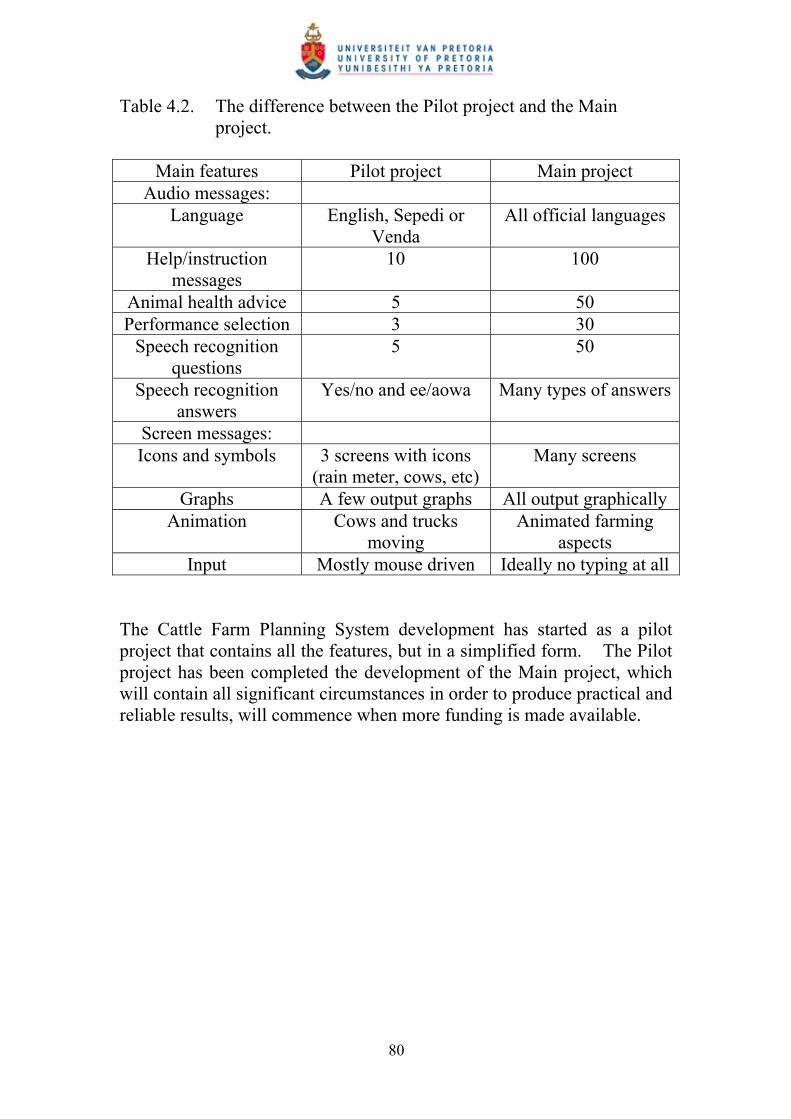
80

Table 4.2. The difference between the Pilot project and the Main project.

Main features Pilot project Main project

Audio messages: Language English, Sepedi or

Venda All official languages

Help/instruction messages

10 100

Animal health advice 5 50 Performance selection 3 30

Speech recognition questions

5 50

Speech recognition answers

Yes/no and ee/aowa Many types of answers

Screen messages: Icons and symbols 3 screens with icons

(rain meter, cows, etc) Many screens

Graphs A few output graphs All output graphically Animation Cows and trucks

moving Animated farming

aspects Input Mostly mouse driven Ideally no typing at all

The Cattle Farm Planning System development has started as a pilot project that contains all the features, but in a simplified form. The Pilot project has been completed the development of the Main project, which will contain all significant circumstances in order to produce practical and reliable results, will commence when more funding is made available.

81

Veld condition

Carrying capacity

Quality

(seasonal) time lag

Pasture manage-

ment

Natural grazing Fodder bank Feed composition Animal production Marketing

Buffer stock Running costs Supplementary

feeds

Farm factors,

soil

Each animal group divided into approximately 12 age groups

Replacement

Calves

Culls

Figure 4.3. A schematic model of beef cattle ranch production. 4.2 Outline of the software program There are three key variables that affect the decisions made by extensive beef farmers. Rainfall is one; drought brings to mind a spectre of starving cattle. However, the variability associated with the beef price cycle may be even more important to the extensive beef farmer. The third key variable is veld condition (Meyer, 1993). The decisions considered in this study concerned the optimum choice of stocking density, cattle system and timing of sales, and the optimum degree of flexibility as regards changes in these decisions from one year to the next. Decisions are evaluated in terms of annual gross margins (Meyer, 1993). The system consists of an extensive farm database, containing specific farm data and elaborate animal data (the type of breed used on each farm). This animal database consists of feed and growth data for each animal group, each gender and also data on fertility, mating and calving

Roughage

Nutrition. value

Feed for: Growth

Maintenance Fattening

Metabolic factors Feed

conversion

Breeding cows

Heifers

Bulls

(mainte-nance)

Oxen

(Growth)

Fattening

Meat prices

(forecast)

Marketing costs

Grain (buy/ grow)

Concen-

trate

Licks

Other

Silage

Hay

Other

Meat heifers

(growth)

Vaccination

Implements

Transport

Labour

Management

Capital

Interest

rate

Inflation

Cash flow

Financial factors

Rainfall (forecast)

82

Replacement

Fertility: 40% calves

Animal Production Marketing Culling (old cows and bulls) R 2000

20% nr = Bm

Strategies:

weaners (9 months) (1)

R 1500 nr = Gm

15 months (9 + 6) (2)

R 2000 nr = Gm

21 months (9 + 12) (3)

R 2500 nr = Gm

percentages. Furthermore, meat prices and all types of costs for each animal age group are stored. Most of this data can be altered by the farmer or user in order to fit his particular circumstances. A very simplistic model was developed for beef cattle production in an extensive farming system (Figure 4.3). This example has no deaths, no fluctuating prices or rainfall effects. Figure 4.4. A mathematical model for beef cattle production under

typical farming circumstances. In this example the farmer has three possible strategies: he can sell all his weaners (thus no growing herd), or sell after six months in the growing herd, or sell after 12 months in the growing herd. The objective of this programme is to find out what the best strategy would be for maximum profit. For all three strategies we must calculate Bh (the number of animals in the breeding herd, Bm (the number of animals from the breeding herd that would be marketed [culled]), Gh (the number of animals in the growing herd) and Gm (the number of animals from the growing herd that would be marketed).

Breeding herd

nr = Bh

Feed: 10 kg/day/animal Running costs: R20 month/animal = R240/year/animal

Growing herd

nr = Gh

Feed: 8 kg/day/animal Running costs: R10/ month/animal = R120/year/animal = R60/6 months/animal

Grazing area 500 ha

Growth: 2 ton/ha/annum = 2*500 = 1000 ton total = 1000/365 ton per day = 3 ton/day = 3000 kg/day

This farmer has 3 possible strategies: 1. Sell weaners (no growing herd; Gh = 0) 2. Sell after 6 months in the growing herd 3. Sell after 12 months in the growing herd QUESTION: Which is the best strategy for maximum profit

83

Profit equations were formed from Figure 4.4: Profit = total sales – total running costs per annum

Thus for strategy (1): 2000*Bm + 1500*Gm – 240*Bh – 0 Strategy (2): 2000*Bm + 1500*Gm – 240*Bh – 60*Gh Strategy (3): 2000*Bm + 1500*Gm – 240*Bh – 120*Gh

The equation with the maximum profit is the best strategy. To simplify the model certain things will be taken for granted. First the total feed that is consumed will be the total feed available per annum. 10*Bh + 8*Gh = 3000 kg (based on a 100 cow herd)/day (equation 1), Secondly 20% of the animals from the breeding herd will be culled, thus there are five times more animals in the herd than those culled.

Bm = 20%*Bh. Thus Bh = 5*Bm (equation 2). Thirdly, 40% fertility means that only 40% of the cows that were mated will calf (40%*Bh), thus out of 100 cows just 40 calves. Further, the number of calves going into the growing herd equals the number of animals going out (marketed) (Gm)

Bm + Gm = 0.4*Bh The last three equations are the same for all strategies, but there is a peculiar relation between the number Gh in the growing herd and the number marketed.

1. Strategy (1): all calves will be marketed immediately, thus there will be no growing herd of cattle. This strategy can be called the weaner strategy.

2. Strategy (2): animals will be kept for 6 months in the herd. Hence, on average only half of the time per annum. The running costs and feed consumption will be half of normal (if you had 100 animals, you will be left with 50, they eat half of what a 100 animals would have eaten).

3. Strategy (3): the animals will be kept for 12 months in the herd. All progeny will be sold each year.

This extremely simple model is unfortunately useless in practice and even the current model is already very complicated to solve. The model consists of only four equations and four variables. Fortunately computer methods, called algorithms, have been developed to help us with this. Instead of the above three strategies, in practice there are millions of possibilities from which the computer finds the best one within a matter of seconds. The basic mathematical model, as it has been developed for the Pilot project consists of a matrix of 206 equations and 412 variables that

84

provides the input for a linear-programming based optimiser. The model in the main project will consist of a matrix of an estimated 800 equations and 1200 variables. The variables represent the number of animals, both male and female, of different age groups in each of the eight seasons, which are in the herd and also a corresponding number to be marketed in order to get maximum profit. The equations represent the herd structure, feed consumption, the ratio of males to females and calving percentages. As a result of the current research presented in this thesis, the growth curves for the different age groups are known. In conjunction with the expected meat prices and the dressing-out percentages, the expected market prices on the hoof are calculated. This data is used to calculate the object function for the optimiser. Parameters that also serve as input to the system as coefficients in the matrix elements are fertility percentages, cow:bull mating ratio and mortality percentages. All percentages are calculated for each animal age group. Other input consists of cost of medicines, licks, concentrates, marketing and transport costs. The major constraint is the expected available grazing in the different seasons, which is calculated from grazing area, soil and grass type, and expected rain and temperature, the last two factors being input which may be varied (El-Niño effects). The current computer system was based on all quantifiable farming factors like rainfall, available grazing, nutritional values, feed to meat conversion, animal growth curves, forecasted feed and meat prices and many more. A mathematical model of beef cattle production was developed. The system was designed for cattle farmers of different backgrounds, taking into account that a farmer generally appreciates reliable, but clear and simple input and output.

85

Farm data (general)

Rainfall

Grazing

Animal general (mass and growth

curves)

Animal specific (number of cattle)

Herd composition

Meat prices (forecast)

Financial (running

cost)

Control/inspection tables

(two year animal mass, growth, prices, cost)

Data bank

Keyboard Mouse

Calculations Output

Tables

Marketing strategy (when,

how many)

Finances (income,

cash flow)

Figure 4.5. A schematic model of a basic cattle farm planning system. The cattle farm planning system uses innovative computer game features to make it suitable and understandable for all types of farmers. It uses on-screen information that is almost completely graphical and symbolic with certain animations. Verbal information will be done by two way audio input and output. The system ‘talks to the farmer’ gives information and asks questions and the farmer ‘talks back’ to the system. A speech recognition system will be developed with agricultural vocabulary (in Sepedi, Venda, Xhosa and Zulu), thus the farmer will interact with the system in his or her own language.

Optimising

Input

Screen

Printer

86

Info control Speakers

Microphone Input to system (coded)

Figure 4.6. A schematic model of the speech recognition unit for a basic

cattle farm planning system. All instructions and information will be audio recorded and presented. The information must however be encouraging and not disciplinary and will be presented as recommendations and questions. The audio and animated information will include advice on dipping, vaccination and performance selection. In general the system may be considered as a farming management game with realistic data, resulting in significant profit increase. 4.2.1 Computer system The cattle farm planning system will be a system driven by Windows application programmes, and thus will be navigated in the same manner. From a user’s perspective, the Cattle Farm Planning System may be divided into three parts: input, optimising and output. The system input works in the following way, after logging on and selecting the considered farm, the system asks for three types of input; the first type is the current herd. After clicking on a specific age group symbol, the user types the number of animals in that group. The second type of input is the rain and temperature (expected). For all seasons in two years, the normally expected rain and temperature is shown together with the calculated expected grazing. The user may now change the rain and temperature values after the corrected expected grazing is calculated. The last type of input is the animal specifications. A three-year-old female animal is used as a large stock unit (450 kg cow). The user may then adapt all the specifications (meat price/kg, costs, etc.) to his wishes. Then the system

Message bank

Info

messages (system help and farming

info)

Questions

Answer bank

Recognition

Answers (voice)

Screen (output)

Animation

Icons

Graphs

Printer symbols

and graphs

87

calculates pro rata the corresponding values for all other animal age groups or gender. These values will be graphically displayed in order to have the user convinced that these input results are relevant and agreeable. These graphical and symbolic displays may be called control tables. When the farmer has convinced himself that the input is realistic, the optimising for maximum profit may start. With the current computer technology and efficient optimising programmes, it will be done in a matter of seconds. With the Pilot project only one maximum profit and corresponding marketing result is calculated. However in practice there are many near optimal solutions and strategies, which must be taken into account. This will be implemented in the main project. When the Main project is developed, other features, such as minimum cash flow, inflation and risk management will also be implemented.

· Installation An installation programme will be used to install the system on the farmer’s computer. To install, the farmer should insert the installation CD into the compact disk drive (normally drive D:). From Windows 98 or 2000 the following steps will be followed:

· Click on the start button. · Click on the run button. · Type D:\INSTALL.EXE. · The installation programme will guide the user through

the rest of the installation. To install the system the following is required: Minimum: Capable of running Windows 98 Pentium 3 500 MHz processor

256.0 MB of RAM GB HD space

Colour monitor Ideally: Capable of running Windows 2000 Pentium 5 800 MHz processor

500 MB of Ram 40.0 GB HD space Colour monitor

88

The average size of the pilot programme files is 50 MB, of which the greatest part is used for images and graphics. The database with animal and farm data is currently about 1 MB. The main project will result in a system not exceeding 100 MB.

· System activities - Log on/off Farm imagery on screen - Data base update Control tables are calculated and

displayed on screen. - Optimising run Calculate planning results

(marketing, herd composition, finances).

- Show tables Control tables and result tables (these only after optimising run).

- Print tables Selective - Animation on/off Screen text off/on - Speech on/off Screen text off/on - Help system Text or speech - Help farming Text or speech - Exit

4.2.2 Programming approach Increased interest among animal scientists and producers in life-time weight-age relationships has been stimulated by the recognition of the economic importance of rate of maturing, rate of gain, mature size and related characters. However, a series of weight-age data points is analytically unwieldy and difficult to interpret. Empirical descriptions of weight-age relationships in cattle provide a technique for reducing the number of variables describing growth and characterizing the form of the growth characteristics. The value of any empirical technique depends upon the accuracy with which it describes the observed data. Unfortunately, the usual tests of goodness of fit may be inaccurate because of correlated errors among longitudinal data points. Therefore, the evaluation of fit was a largely subjective approach in which the plots of observed and predicted weights were compared (Brown et al, 1976). The majority of cattle in Africa show Zebu parentage (Squires and Vera, 1992). Brahman and Nguni cattle data was used for the pilot study. Most of the developing farmers had either this type of cattle, or a crossbred herd with Brahman and other types of cattle. Crossbreeding generally refers to the systematic blending of Bos taurus and Bos indicus genes in

89

order to combine genes for tropical adaptability (Bos indicus) with those favourable for high growth rate and good carcass quality (Bos taurus) (Renand et al, 1992). Nguni cattle are climatised to warm areas with relatively high humidities. These cattle are kept extensively. They are cattle of medium size, with a fair depth of body, fairly short legs and a tendency towards the wedge shaped ‘dairy type’. Nguni cattle are maintained for the production of crossbred beef, milk for local consumption and in some cases as draft animals (Joshi et al, 1957). The Bos indicus species of cattle, such as the Brahman of the Americas and Asia is well adapted to sub tropic and semi-arid regions. They are sleek-coated, have a large surface area per unit mass and a fairly well developed dewlap and sheath or navel fold. They are also thick of hide; the blood flow to the hide is profuse and thus will help them to be adapted to high temperatures (Bonsma, 1980). Weight gain has a direct influence on the income of the commercial beef producer, and he should therefore strive to obtain maximum weight gains (Department of Agricultural Technical Services, 1965). Using data that was found in Bosman (1997), Kreiner (1990) and Preston and Willis (1970) a graph (Figure 4.7) was drawn for female animals in optimum condition. A confidence interval of 10% was used to determine under and over conditioned animals, thus 5% above the optimum would be over conditioned and 5% under the optimum would be under conditioned.

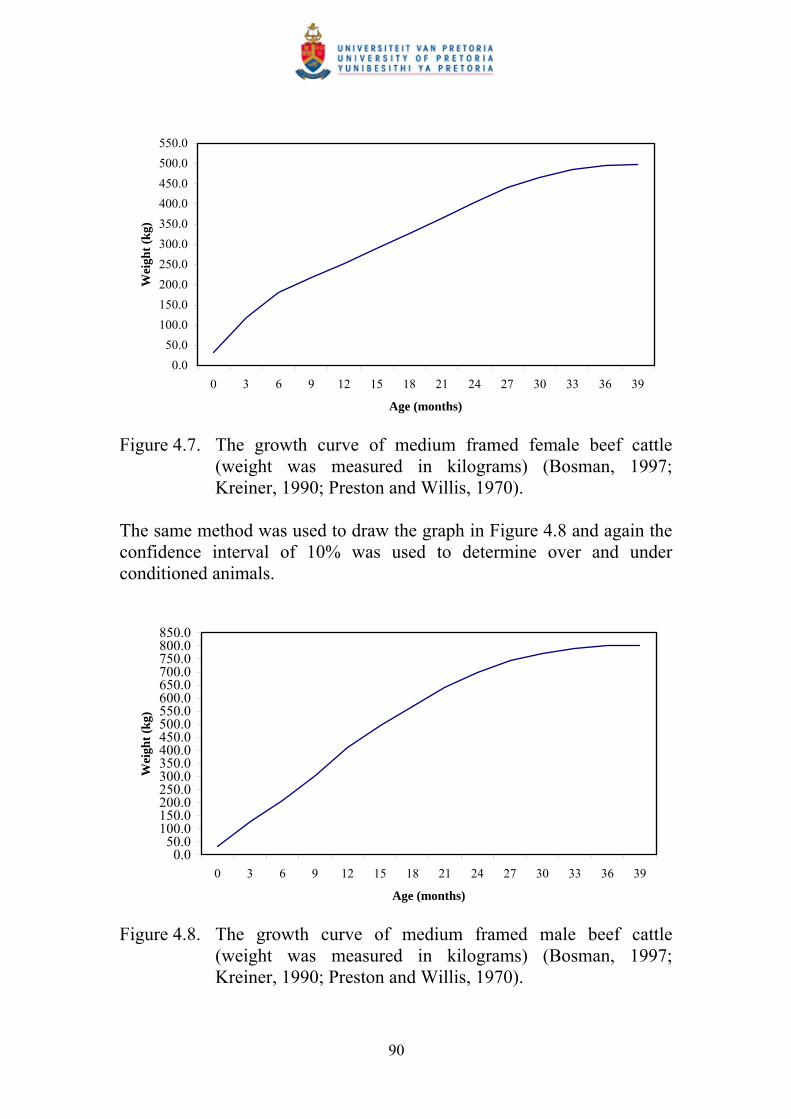
90

0.0

50.0

100.0

150.0

200.0

250.0

300.0

350.0

400.0

450.0

500.0

550.0

0 3 6 9 12 15 18 21 24 27 30 33 36 39

Age (months)

Wei

ght

(kg)

Figure 4.7. The growth curve of medium framed female beef cattle

(weight was measured in kilograms) (Bosman, 1997; Kreiner, 1990; Preston and Willis, 1970).

The same method was used to draw the graph in Figure 4.8 and again the confidence interval of 10% was used to determine over and under conditioned animals.

0.050.0

100.0150.0200.0250.0300.0350.0400.0450.0500.0550.0600.0650.0700.0750.0800.0850.0

0 3 6 9 12 15 18 21 24 27 30 33 36 39

Age (months)

Wei

ght

(kg)

Figure 4.8. The growth curve of medium framed male beef cattle

(weight was measured in kilograms) (Bosman, 1997; Kreiner, 1990; Preston and Willis, 1970).

91

Table 4.3. Weights of medium framed beef cattle in kilograms with different condition levels and varying ages (plotted from Figure 4.7 and Figure 4.8).

Ages of animals in months C o n d i t i o n

l e v e l s 0 3 6 9 12 15 18 21 24 27 30 33 36 39+ U n d e r

c o n d i t i o n e d 31.1 114.0 171.0 206.2 240.4 275.4 309.7 346.8 383.5 417.7 443.4 460.8 470.3 472.2 O p t i m u m c o n d i t i o n 32.7 120.0 180.0 217.0 253.0 289.9 326.0 365.0 403.7 439.7 466.7 485.0 495.0 497.0

Female animals

O v e r c o n d i t i o n e d 34.3 126.0 189.0 227.9 265.7 304.4 342.3 383.3 423.9 461.7 490.0 509.3 519.8 521.9

U n d e r c o n d i t i o n e d 31.4 119.7 196.7 290.7 388.6 470.3 541.1 609.5 664.2 705.3 733.5 750.6 760.0 761.9

O p t i m u m c o n d i t i o n 33.0 126.0 207.0 306.0 409.0 495.0 569.6 641.6 699.2 742.4 772.1 790.1 800.0 802.0

Male animals

O v e r c o n d i t i o n e d 34.7 132.3 217.4 321.3 429.5 519.8 598.1 673.7 734.2 779.5 810.7 829.6 840.0 842.1

Steer calves gain 6% more on pasture than do heifer calves (Louw et al, 1992). The average daily gain (Table 4.4) was calculated by the following equation: The initial and end weights of the animals are taken from the data in Table 4.3. Table 4.4. Average daily gain in kilograms of medium framed beef

cattle (male and female) with different condition levels and varying ages (derived from Table 4.3).

Ages of animals in months C o n d i t i o n

l e v e l s 0 3 6 9 12 15 18 21 24 27 30 33 36 39+

U n d e r c o n d i t i o n e d 0.92 0.63 0.39 0.38 0.39 0.38 0.41 0.41 0.38 0.29 0.19 0.11 0.02

O p t i m u m c o n d i t i o n 0.97 0.67 0.41 0.40 0.41 0.40 0.43 0.43 0.40 0.30 0.20 0.11 0.02

Female animals

O v e r c o n d i t i o n e d 1.02 0.70 0.43 0.42 0.43 0.42 0.46 0.45 0.42 0.32 0.21 0.12 0.02

U n d e r c o n d i t i o n e d 0.98 0.86 1.05 1.09 0.91 0.79 0.76 0.61 0.46 0.31 0.19 0.10 0.02

O p t i m u m c o n d i t i o n 1.03 0.90 1.10 1.14 0.96 0.83 0.80 0.64 0.48 0.33 0.20 0.11 0.02

Male animals

O v e r c o n d i t i o n e d 1.09 0.95 1.16 1.20 1.00 0.87 0.84 0.67 0.50 0.35 0.21 0.12 0.02

In designing breeding programmes for beef cattle, it is important to know the genetic relationships between early growth and mature size, as well as rate of maturing (Meyer, 1995). The following procedure was used to draw Table 4.5: Data from NRC (1984) and NRC (1996) was used to draw a regression line in order to

End weight of animal for a period – initial weight of animal for a period Average daily gain = Amount of days in a period

92

calculate values for all the different cells in Table 4.5. The regression equation for the data is:

y = 3.2704(Lnx) - 2.3638

the R2-value was 0.95. That means that the regression line fits the data by 95%. Table 4.5. The dry matter intakes (kg/day) of medium framed beef

cattle (female) of varying condition levels for maintenance (values determined by regression equation).

Ages of animals in months Condition levels 0 3 6 9 12 15 18 21 24 27 30 33 36 39+

Under conditioned 1.17 3.32 4.58 5.47 6.17 6.73 7.21 7.63 7.99 8.32 8.62 8.89 9.14 Optimum condition 1.23 3.50 4.82 5.76 6.49 7.09 7.59 8.03 8.41 8.76 9.07 9.36 9.62

Over conditioned 1.29 3.67 5.06 6.05 6.82 7.44 7.97 8.43 8.84 9.20 9.52 9.82 10.10 y = 3.2704(Lnx) - 2.3638 R2 = 0.95

The following procedure was used to draw Table 4.6. Data from NRC (1984) and NRC (1996) was used to draw a regression line in order to calculate values for all the different cells in Table 4.6. The regression equation for the data was:

y = 3.8169(Lnx) – 1.2044

the R2-value was 0.99. That means that the regression line fits the data by 99%. Table 4.6. The dry matter intakes (kg/day) of medium framed beef

cattle (male) of varying condition levels for maintenance (values determined by regression equation).

Ages of animals in months Condition levels 0 3 6 9 12 15 18 21 24 27 30 33 36 39+

Under conditioned 2.84 5.35 6.82 7.87 8.68 9.34 9.90 10.38 10.81 11.19 11.53 11.85 12.14 Optimum condition 2.99 5.63 7.18 8.28 9.13 9.83 10.42 10.93 11.38 11.78 12.14 12.47 12.78 Over conditioned 3.14 5.92 7.54 8.69 9.59 10.32 10.94 11.47 11.94 12.37 12.75 13.10 13.42

y = 3.8169(Lnx) – 1.2044 R2 = 0.99

The voluntary forage intake of beef cows is determined by a number of factors related to the cows themselves, i.e. their feed intake capacity, to the intrinsic characteristics of the forages used and to environment. Feed intake ranges from less than 1.5 kg to more than 2.5 kg of dry matter per 100 kg live weight. The intake capacity decreases slightly (by 5 to 10%) during the last 2 weeks of pregnancy, probably because of the combined effects of physical limitation of the rumen volume by the conceptus and

93

fat, and of metabolic and hormonal changes before parturition. The intake capacity is also decreased by fatness (Petit et al, 1992). The following procedure was used to draw Table 4.7: Data from NRC (1984), NRC (1996) and ARC (1980) was used to draw a regression line in order to calculate values for all the different cells in Table 4.7. The regression equation for the data is:

y = 4.6051(Lnx) - 4.8776

the R2-value was 0.99. That means that the regression line fits the data with 99% accuracy. Table 4.7. The dry matter intakes (kg/day) above maintenance of

medium framed beef cattle (female) with different condition levels and varying ages (values determined by using a regression equation).

Ages of animals in months Condition

levels 0 3 6 9 12 15 18 21 24 27 30 33 36 39+ Under

conditioned 1.19 3.21 4.98 6.24 7.21 8.01 8.69 9.27 9.79 10.25 10.66 11.04 11.39

Optimum condition 1.25 3.37 5.24 6.57 7.59 8.43 9.14 9.76 10.30 10.79 11.22 11.63 11.99

Over conditioned 1.31 3.54 5.50 6.89 7.97 8.85 9.60 10.25 10.82 11.32 11.79 12.21 12.59 y = 4.6051(Lnx) - 4.8776 R2 = 0.99

Generally, veld grazing provides the cheapest source of roughage with which to grow out, and finish beef steers, albeit over relatively long periods (two to three years), and at relatively low levels of gain per unit area (Louw, 1992). It is imperative that mating bulls are subject to sound nutritional programmes so that they are in a sound working condition prior to breeding. Hard working bulls tend to draw on their body reserves during the breeding season, emphasising the need for a sound pre-season body condition. To achieve this, mature bulls need approximately 1kg hay (or 3 kg of maize silage), plus 1 to 1.5 kg of concentrate per 100 kg of body mass (Crichton, 1992). The following procedure was used to draw Table 4.8: Data from NRC (1984), NRC (1996) and ARC (1980) was used to draw a regression line in order to calculate values for all the different cells in Table 4.8. The regression equation for the data was:

y = 5.1457(Lnx) - 3.7054

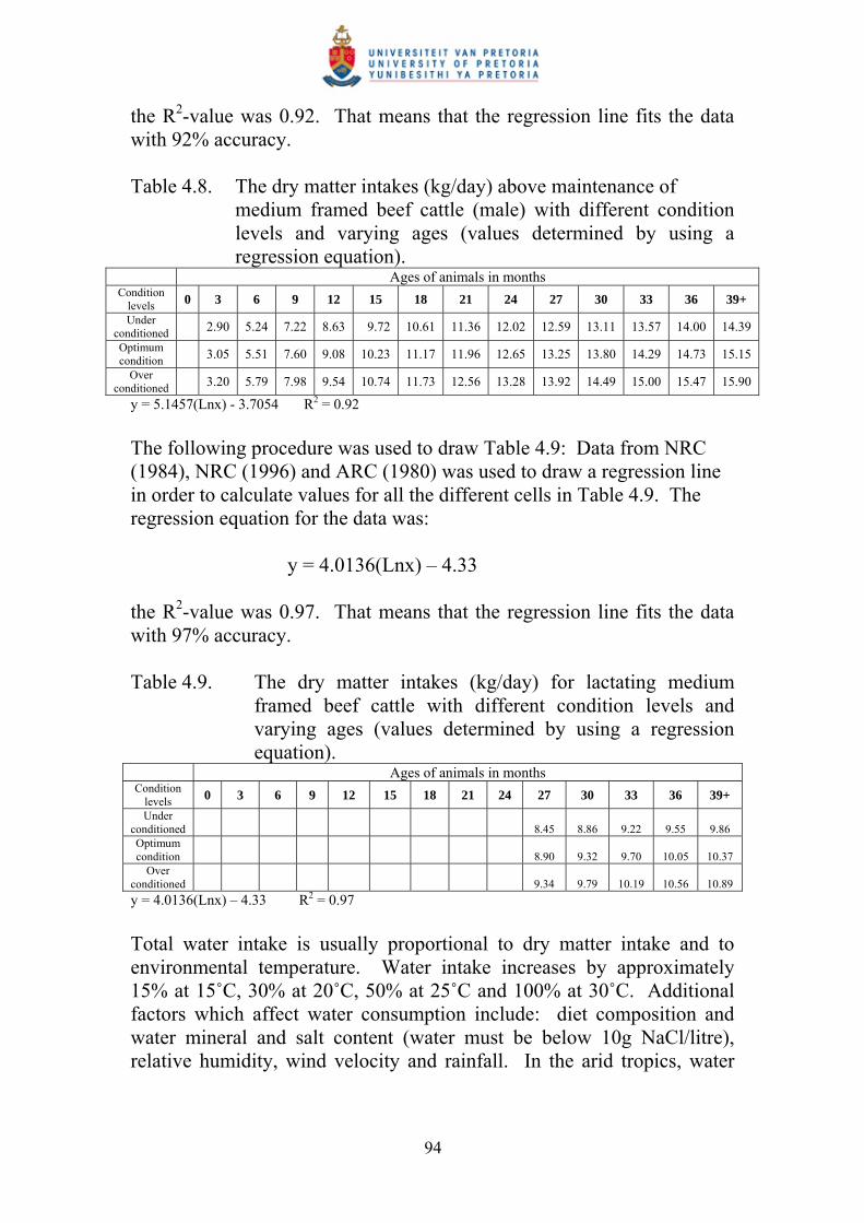
94

the R2-value was 0.92. That means that the regression line fits the data with 92% accuracy. Table 4.8. The dry matter intakes (kg/day) above maintenance of

medium framed beef cattle (male) with different condition levels and varying ages (values determined by using a regression equation).

Ages of animals in months Condition

levels 0 3 6 9 12 15 18 21 24 27 30 33 36 39+

Under conditioned 2.90 5.24 7.22 8.63 9.72 10.61 11.36 12.02 12.59 13.11 13.57 14.00 14.39

Optimum condition 3.05 5.51 7.60 9.08 10.23 11.17 11.96 12.65 13.25 13.80 14.29 14.73 15.15

Over conditioned 3.20 5.79 7.98 9.54 10.74 11.73 12.56 13.28 13.92 14.49 15.00 15.47 15.90

y = 5.1457(Lnx) - 3.7054 R2 = 0.92

The following procedure was used to draw Table 4.9: Data from NRC (1984), NRC (1996) and ARC (1980) was used to draw a regression line in order to calculate values for all the different cells in Table 4.9. The regression equation for the data was:

y = 4.0136(Lnx) – 4.33

the R2-value was 0.97. That means that the regression line fits the data with 97% accuracy. Table 4.9. The dry matter intakes (kg/day) for lactating medium

framed beef cattle with different condition levels and varying ages (values determined by using a regression equation).

Ages of animals in months Condition

levels 0 3 6 9 12 15 18 21 24 27 30 33 36 39+

Under conditioned 8.45 8.86 9.22 9.55 9.86 Optimum condition 8.90 9.32 9.70 10.05 10.37

Over conditioned 9.34 9.79 10.19 10.56 10.89

y = 4.0136(Lnx) – 4.33 R2 = 0.97

Total water intake is usually proportional to dry matter intake and to environmental temperature. Water intake increases by approximately 15% at 15˚C, 30% at 20˚C, 50% at 25˚C and 100% at 30˚C. Additional factors which affect water consumption include: diet composition and water mineral and salt content (water must be below 10g NaCl/litre), relative humidity, wind velocity and rainfall. In the arid tropics, water

95

%Water in feed

Free water consumption (litre) = Total water (litre) - % Dry matter in feed * Daily dry matter intake in grams Weight of water in grams per litre

intake is 45% greater in summer than in winter owing to use of water for evaporative cooling (Owens and Geay, 1992). Water intake is a function of dry matter consumption. Water intake per unit of dry matter ingested remains relatively constant from around –12˚C to 4˚C (10˚F to 40˚F), and then increases with ambient temperature at an accelerating rate. In Figure 4.9 the given mean values of total water intake in litres per 454g of dry matter ingested at 4˚C to 38˚C (Winchester and Morris, 1956).

0

1

2

3

4

5

6

7

8

4 10 16 21 27 32 38 Ambient temperature

*Per 454g of dry matter ingested

Wat

er in

tak

e *

European cattle

Indian cattle

Figure 4.9. Water intake expressed as a function of dry matter

consumption and ambient temperature (Winchester and Morris, 1956).

The information presented in Figure 4.9 is given in terms of total water intake (per animal per day) which includes both the water drunk and the water contained in the feed. The amount of free water that cattle can be expected to drink can be calculated by using the following equation (Winchester and Morris, 1956): If salt was added to the diet in an attempt to double the water intake, the water consumption was raised by 40 to 60%. Until the ambient

96

temperature exceeds 26˚C, cattle tend to do most of their drinking in the late morning and late afternoon and evening. Very little water is consumed during the night or in the early morning and early afternoon hours. At 32˚C, the periods during which no water is consumed tend to be shortened and it appears that the animals then tend to drink every 2 hours or more often (Winchester and Morris, 1956). The data in Table 4.10 was calculated by using the following equation: y = -19.76 + (0.4202*MT) + (0.1329*DMI) - (6.5966*PP) - (1.1739*DS) where MT is the maximum temperature in degrees Fahrenheit, DMI is the dry matter intake per day of the animal, PP is the precipitation level in this specific area, DS is the percentage salt in the animals diet (NRC, 1996). Table 4.10. Water requirements (litre/animal/day) of medium framed

beef cattle (male and female), with different condition levels and varying ages at a temperature of 28 degrees Celsius and a precipitation value of 2.57 (NRC, 1996).

Ages of animals in months Condition

levels 0 3 6 9 12 15 18 21 24 27 30 33 36 39+

Under conditioned

5.63 16.64 24.21 28.87 33.41 38.06 42.61 47.53 52.41 56.95 60.35 62.66 63.92 64.18

Optimum condition

5.85 17.44 25.40 30.31 35.09 39.99 44.78 49.95 55.09 59.87 63.45 65.88 67.21 67.47 Female animals

Over conditioned

6.07 18.23 26.59 31.75 36.77 41.91 46.94 52.38 57.77 62.79 66.55 69.10 70.49 70.77

Under conditioned

2.09 17.40 27.61 40.09 53.08 63.92 73.33 82.41 89.67 95.12 98.86 101.13 102.38 102.63

Optimum condition

2.31 18.23 28.98 42.12 55.79 67.21 77.11 86.67 94.31 100.04 103.99 106.37 107.69 107.95 Male

animals Over

conditioned 2.53 19.07 30.36 44.15 58.51 70.49 80.89 90.92 98.95 104.97 109.11 111.62 113.00 113.28

y = -19.76 + (0.4202*MT) + (0.1329*DMI) - (6.5966*PP) - (1.1739*DS) MT=maximum temperature in degrees Fahrenheit, DMI=dry matter intake per day, PP=precipitation, DS=diet salt %

The following procedure was used to draw Table 4.11: Data from Preston and Willis (1970) was used to draw a regression line in order to calculate values for all the different cells in Table 4.11. The regression equation for the data was:

y = 50.632(power(x,0.0911)

the R2-value was 0.9392. That means that the regression line fits the data with 94% accuracy.

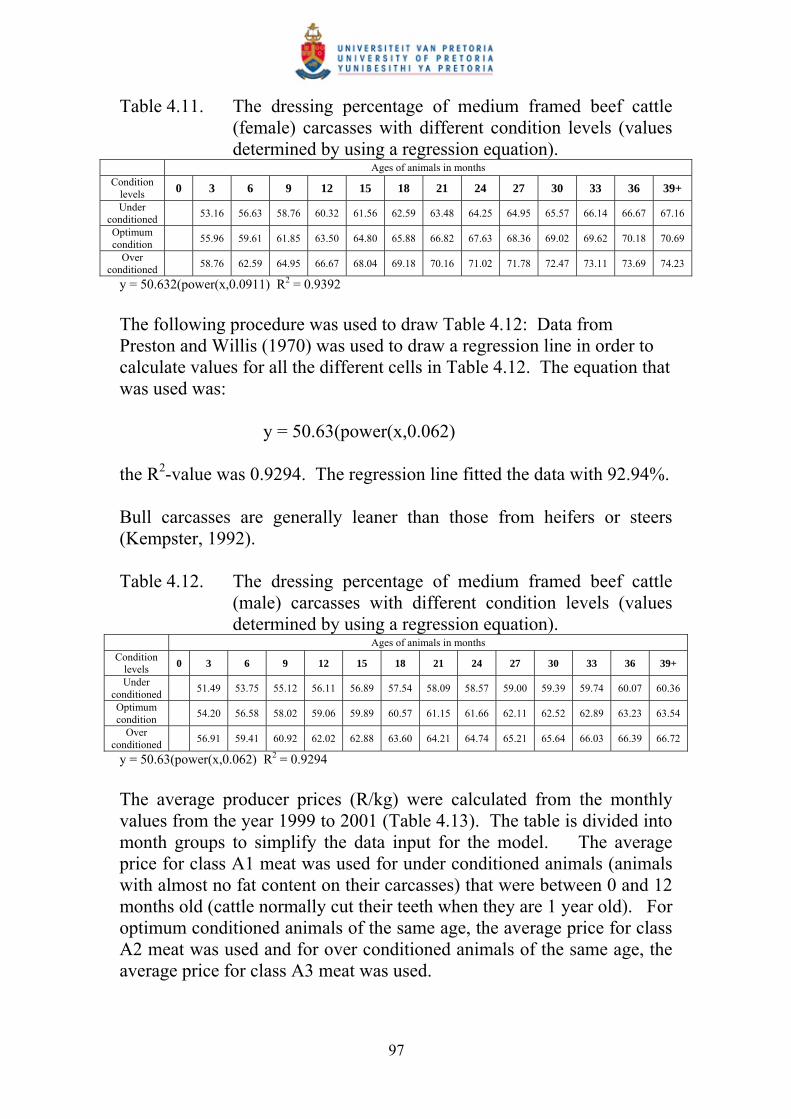
97

Table 4.11. The dressing percentage of medium framed beef cattle (female) carcasses with different condition levels (values determined by using a regression equation).

Ages of animals in months Condition

levels 0 3 6 9 12 15 18 21 24 27 30 33 36 39+

Under conditioned

53.16 56.63 58.76 60.32 61.56 62.59 63.48 64.25 64.95 65.57 66.14 66.67 67.16

Optimum condition

55.96 59.61 61.85 63.50 64.80 65.88 66.82 67.63 68.36 69.02 69.62 70.18 70.69

Over conditioned

58.76 62.59 64.95 66.67 68.04 69.18 70.16 71.02 71.78 72.47 73.11 73.69 74.23

y = 50.632(power(x,0.0911) R2 = 0.9392

The following procedure was used to draw Table 4.12: Data from Preston and Willis (1970) was used to draw a regression line in order to calculate values for all the different cells in Table 4.12. The equation that was used was:

y = 50.63(power(x,0.062)

the R2-value was 0.9294. The regression line fitted the data with 92.94%. Bull carcasses are generally leaner than those from heifers or steers (Kempster, 1992). Table 4.12. The dressing percentage of medium framed beef cattle

(male) carcasses with different condition levels (values determined by using a regression equation).

Ages of animals in months Condition

levels 0 3 6 9 12 15 18 21 24 27 30 33 36 39+

Under conditioned

51.49 53.75 55.12 56.11 56.89 57.54 58.09 58.57 59.00 59.39 59.74 60.07 60.36

Optimum condition

54.20 56.58 58.02 59.06 59.89 60.57 61.15 61.66 62.11 62.52 62.89 63.23 63.54

Over conditioned

56.91 59.41 60.92 62.02 62.88 63.60 64.21 64.74 65.21 65.64 66.03 66.39 66.72

y = 50.63(power(x,0.062) R2 = 0.9294

The average producer prices (R/kg) were calculated from the monthly values from the year 1999 to 2001 (Table 4.13). The table is divided into month groups to simplify the data input for the model. The average price for class A1 meat was used for under conditioned animals (animals with almost no fat content on their carcasses) that were between 0 and 12 months old (cattle normally cut their teeth when they are 1 year old). For optimum conditioned animals of the same age, the average price for class A2 meat was used and for over conditioned animals of the same age, the average price for class A3 meat was used.

98

Then for the 1 to 2 year old animals the average price for class AB1 (under conditioned animals), AB2 (optimum conditioned animals) and AB3 (over conditioned animals) were calculated. And the animals older than that were divided into groups that have the average prices for: C1 (under conditioned animals), C2 (optimum conditioned animals) and C3 (over conditioned animals) meat. At the time of the study the values for the months June to December for the year 2001 were not available and were not used in this calculation. Table 4.13. The average producer prices (R/kg) of beef cattle (SAMIC).

Ages of animals in months Condition

levels 0 3 6 9 12 15 18 21 24 27 30 33 36 39+

Under conditioned

8.62 8.62 8.62 8.62 8.25 8.25 8.25 8.25 7.91 7.91 7.91 7.91 7.91 7.91

Optimum condition

8.87 8.87 8.87 8.87 8.45 8.45 8.45 8.45 8.09 8.09 8.09 8.09 8.09 8.09 October to December

Over conditioned

8.87 8.87 8.87 8.87 8.48 8.48 8.48 8.48 8.05 8.05 8.05 8.05 8.05 8.05

Under conditioned

8.91 8.91 8.91 8.91 8.41 8.41 8.41 8.41 8.01 8.01 8.01 8.01 8.01 8.01

Optimum condition

9.24 9.24 9.24 9.24 8.70 8.70 8.70 8.70 8.29 8.29 8.29 8.29 8.29 8.29 January to

March Over

conditioned 9.22 9.22 9.22 9.22 8.65 8.65 8.65 8.65 8.22 8.22 8.22 8.22 8.22 8.22

Under conditioned

8.95 8.95 8.95 8.95 8.45 8.45 8.45 8.45 8.01 8.01 8.01 8.01 8.01 8.01

Optimum condition

9.13 9.13 9.13 9.13 8.62 8.62 8.62 8.62 8.16 8.16 8.16 8.16 8.16 8.16 April to

June Over

conditioned 9.06 9.06 9.06 9.06 8.47 8.47 8.47 8.47 8.09 8.09 8.09 8.09 8.09 8.09

Under conditioned

8.73 8.73 8.73 8.73 8.41 8.41 8.41 8.41 7.97 7.97 7.97 7.97 7.97 7.97

Optimum condition

8.85 8.85 8.85 8.85 8.59 8.59 8.59 8.59 8.13 8.13 8.13 8.13 8.13 8.13 July to

September Over

conditioned 8.81 8.81 8.81 8.81 8.52 8.52 8.52 8.52 8.05 8.05 8.05 8.05 8.05 8.05

The economic margin of meat wholesalers depends on other characteristics, such as carcass yield, weight at the optimum level of fatness, carcass composition and conformation. These traits determine the saleable meat in the slaughtered cattle and the relative amount of higher-priced cuts. In general, retailers tend to favour carcasses with good muscle conformation, but emphasis laid on that trait widely depends on consumer habits (Renand et al, 1992). The market prices (Table 4.14) of beef cattle on the hoof were calculated by multiplying the average producer prices (Table 4.13) of the animals, with the dressing percentages (Table 4.11) of these animals for a specific age group.

99

Table 4.14. The average market prices (R/animal) of beef cattle (male and female) on the hoof (derived from Table 4.11).

Ages of animals in months Condition

levels 0 3 6 9 12 15 18 21 24 27 30 33 36 39+ Under

conditioned 4.58 4.88 5.07 4.98 5.08 5.17 5.24 5.08 5.14 5.19 5.23 5.27 5.31

Optimum condition

4.96 5.29 5.49 5.36 5.47 5.56 5.64 5.47 5.53 5.58 5.63 5.67 5.72

October to December for female

animals Over conditioned

5.21 5.55 5.76 5.65 5.77 5.86 5.95 5.72 5.78 5.84 5.89 5.93 5.98

Under conditioned

4.44 4.63 4.75 4.63 4.70 4.75 4.79 4.63 4.67 4.70 4.73 4.75 4.77

Optimum condition

4.81 5.02 5.15 4.99 5.06 5.11 5.16 4.99 5.02 5.05 5.08 5.11 5.14

October to December for male animals Over

conditioned 5.05 5.27 5.40 5.26 5.33 5.39 5.44 5.21 5.25 5.29 5.32 5.35 5.37

Under conditioned

4.73 5.04 5.23 5.07 5.18 5.26 5.34 5.15 5.20 5.25 5.30 5.34 5.38

Optimum condition

5.17 5.51 5.71 5.52 5.64 5.73 5.81 5.61 5.67 5.72 5.77 5.82 5.86

January to March for

female animals Over

conditioned 5.42 5.77 5.99 5.77 5.89 5.99 6.07 5.84 5.90 5.96 6.01 6.06 6.10

Under conditioned

4.59 4.79 4.91 4.72 4.78 4.84 4.89 4.69 4.73 4.76 4.79 4.81 4.84

Optimum condition

5.01 5.23 5.36 5.14 5.21 5.27 5.32 5.11 5.15 5.18 5.21 5.24 5.27

January to March for

male animals Over

conditioned 5.25 5.48 5.62 5.37 5.44 5.50 5.56 5.32 5.36 5.40 5.43 5.46 5.48

Under conditioned

4.76 5.07 5.26 5.10 5.20 5.29 5.36 5.15 5.20 5.25 5.30 5.34 5.38

Optimum condition

5.11 5.44 5.65 5.47 5.59 5.68 5.76 5.52 5.58 5.63 5.68 5.72 5.77

April to June for female animals Over

conditioned 5.33 5.67 5.89 5.65 5.76 5.86 5.94 5.75 5.81 5.86 5.92 5.96 6.01

Under conditioned

4.61 4.81 4.93 4.74 4.81 4.86 4.91 4.69 4.73 4.76 4.79 4.81 4.84

Optimum condition

4.95 5.16 5.30 5.09 5.16 5.22 5.27 5.03 5.07 5.10 5.13 5.16 5.18

April to June for

male animals Over

conditioned 5.16 5.38 5.52 5.25 5.33 5.39 5.44 5.24 5.28 5.31 5.34 5.37 5.40

Under conditioned

4.64 4.94 5.13 5.07 5.18 5.26 5.34 5.12 5.18 5.23 5.27 5.31 5.35

Optimum condition

4.95 5.28 5.47 5.45 5.56 5.66 5.74 5.50 5.56 5.61 5.66 5.71 5.75

July to September for female

animals Over conditioned

5.17 5.51 5.72 5.68 5.80 5.89 5.98 5.72 5.78 5.84 5.89 5.93 5.98

Under conditioned

4.49 4.69 4.81 4.72 4.78 4.84 4.88 4.67 4.70 4.73 4.76 4.79 4.81

Optimum condition

4.80 5.01 5.13 5.07 5.14 5.20 5.25 5.02 5.05 5.09 5.12 5.14 5.17

July to September for male animals Over

conditioned 5.01 5.23 5.37 5.28 5.36 5.42 5.47 5.21 5.25 5.29 5.32 5.35 5.37

Perinatal calf losses average 5 – 10% and can be higher under range conditions. Most of the difficulties at birth result from excessive calf size for the pelvic area of the cow causing dystocia. Calves born to heifers and young cows are associated with more frequent dystocia; it is also increased in over fat heifers before calving (Thimonier and Signoret, 1992).

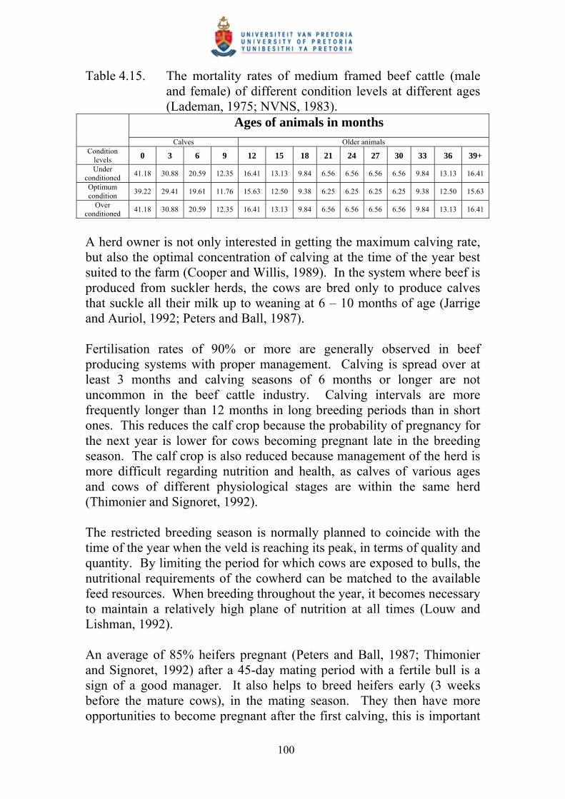
100

Table 4.15. The mortality rates of medium framed beef cattle (male and female) of different condition levels at different ages (Lademan, 1975; NVNS, 1983).

Ages of animals in months

Calves Older animals Condition

levels 0 3 6 9 12 15 18 21 24 27 30 33 36 39+

Under conditioned

41.18 30.88 20.59 12.35 16.41 13.13 9.84 6.56 6.56 6.56 6.56 9.84 13.13 16.41

Optimum condition

39.22 29.41 19.61 11.76 15.63 12.50 9.38 6.25 6.25 6.25 6.25 9.38 12.50 15.63

Over conditioned

41.18 30.88 20.59 12.35 16.41 13.13 9.84 6.56 6.56 6.56 6.56 9.84 13.13 16.41

A herd owner is not only interested in getting the maximum calving rate, but also the optimal concentration of calving at the time of the year best suited to the farm (Cooper and Willis, 1989). In the system where beef is produced from suckler herds, the cows are bred only to produce calves that suckle all their milk up to weaning at 6 – 10 months of age (Jarrige and Auriol, 1992; Peters and Ball, 1987). Fertilisation rates of 90% or more are generally observed in beef producing systems with proper management. Calving is spread over at least 3 months and calving seasons of 6 months or longer are not uncommon in the beef cattle industry. Calving intervals are more frequently longer than 12 months in long breeding periods than in short ones. This reduces the calf crop because the probability of pregnancy for the next year is lower for cows becoming pregnant late in the breeding season. The calf crop is also reduced because management of the herd is more difficult regarding nutrition and health, as calves of various ages and cows of different physiological stages are within the same herd (Thimonier and Signoret, 1992). The restricted breeding season is normally planned to coincide with the time of the year when the veld is reaching its peak, in terms of quality and quantity. By limiting the period for which cows are exposed to bulls, the nutritional requirements of the cowherd can be matched to the available feed resources. When breeding throughout the year, it becomes necessary to maintain a relatively high plane of nutrition at all times (Louw and Lishman, 1992). An average of 85% heifers pregnant (Peters and Ball, 1987; Thimonier and Signoret, 1992) after a 45-day mating period with a fertile bull is a sign of a good manager. It also helps to breed heifers early (3 weeks before the mature cows), in the mating season. They then have more opportunities to become pregnant after the first calving, this is important

101

because the interval from calving to the breeding season is longer (Thimonier and Signoret, 1992). A very high proportion of ova produced at ovulation become fertilised, but many embryos are lost during the early days of pregnancy. By day 19 only 60 to 65% of cows are still pregnant and by day 40, only about 55 to 60%. Therefore 30 to 35% of embryos are lost during the first 40 days of pregnancy (Peters and Ball, 1987). Table 4.16. The percentage heifers and cows in calf in a beef

production system (Meaker, 1984; Crichton, 1992). Ages of animals in months Condition

levels 0 3 6 9 12 15 18 21 24 27 30 33 36 39+

Under conditioned

0.00 0.00 0.00 0.00 19.00 28.50 42.75 47.50 61.75 79.99 79.99 79.99 79.99 79.99

Optimum condition

0.00 0.00 0.00 0.00 20.00 30.00 45.00 50.00 65.00 84.20 84.20 84.20 84.20 84.20

Over conditioned

0.00 0.00 0.00 0.00 19.00 28.50 42.75 47.50 61.75 79.99 79.99 79.99 79.99 79.99

According to daily sperm production and libido, it is possible to join one adult bull to 30 to 40 cows or heifers in pasture mating or 80 to 120 in hand mating (4 to 12 services per week). However, regarding their sperm production, they have to be given only a small number of females to ensure normal fertility and one has to be sure that they are physically able to mate adult beef cows (Thimonier and Signoret, 1992). It is advised to use young bulls conservatively during their first season (Crichton, 1992). For optimum mating capability it is recommended by Crichton (1992) to put:

· Bulls 12 months old with only 10 to 20 cows.

· Bulls 18 months old with 20 to 25 cows.

· Bulls 24 months and older with 25 to 30 cows. Table 4.17. The cow:bull ratio in a beef production system (Meaker,

1984; Crichton, 1992). Ages of animals in months 0 3 6 9 12 15 18 21 24 27 30 33 36 39+

Cows per bull

10 12 20 25 25 28 30 30 30 30

An optimal fertility is the first obvious criterion expected from the breeding bull. Thus, it has to be able to seek out and mate the largest possible number of females. To successfully impregnate them, he has to produce high quality semen. An early puberty is important to take benefit of genetic improvement in reducing the interval between generations.

102

Finally the bull has not only a short-term effect on pregnancy rate, but also a long term one as various components of fertility are inherited. In the selection process the following are important:

- Serving capacity - Physical aptitude and health - Semen production (Thimonier and Signoret, 1992).

Bulls should ideally be tested for semen quality and quantity, physical soundness, lack of reproductive disorders, sex drive and mating ability (Crichton, 1992). It is generally recommended that when the size of the herd is kept constant, about 20% of the breeding herd should be replaced by young breeding stock every year. The rule of thumb is to breed heifers when their body mass is 65% of their estimated mature mass. Select at least 25% more heifers than are actually required for replacement (Van Niekerk and Lishman, 1992). Cull heifers that are empty at the time of pregnancy diagnoses. Cows that miss in consecutive or alternate years should also be considered for culling, as well as old cows that have a declining production (Gammon, 1992b). The main problem with this strict culling programme is that conception rates have to be at least 85%, and that weaning rates have to be at least 70% to be able to produce sufficient replacement heifers, merely to maintain cow numbers (Paterson, 1992). Table 4.18. The distribution of medium framed beef cattle in a herd of

366 animals of different sexes in the herd (Meaker, 1984; Jacobs, 1992b; Production Matters)

Ages of animals in months

Animal’s sex 3 4 5 6 7 8 9 10 11 12 15 18 21 24 39 Cows 75 75 25 25 25 25 25 25 25 25 Bulls 2 2 3 3 3 3

Supplementation limits excessive live weight losses during the dry season (Chenost and Preston, 1992). To make the most of sour veld and mixed veld supplementation with protein, and/or energy, and/or minerals such as phosphorus is necessary, depending on the time of year, and the required level of performance (Gammon, 1992a). Energy supplementation should not be attempted unless a careful study is first made of the subject, and then good management must be applied, otherwise it will usually result in a loss (Jacobs, 1992a).

103

The following licks can be provided for rapidly growing animals on pastures. On ryegrass: 50% salt and 50% dicalciumphosphate. On Kikuyu: 40% salt, 25% feed lime, 25% dicalciumphosphate and 10% molasses powder (Louw, 1992). Three different licks were used for this study (Table 4.19). For the September to February interval only phosphate licks were provided for the animals. This lick consisted of 25% urea, 25% maize meal, 25% dicalciumphosphate and 25% salt. For the March to May period a production lick was provided which consisted of 100 kg monocalciumphosphate, 100 kg urea, 360 kg maize meal, 250 kg calorie 3000 and 200 kg salt. For the June to August period, which is also a very dry period, a maintenance lick was provided consisting of 7% urea, 8% dicalciumphosphate, 20% salt and 65% molasses. The prices for the different raw elements were for the year 2001.

104

Table 4.19. Calculation of the lick costs (R/animal/ month) of medium framed beef cattle (female) for the year 2001, based on the metodology of Jacobs (1992c) and Van Niekerk (1975).

Ages of animals in months Condition

levels 0 3 6 9 12 15 18 21 24 27 30 33 36 39+

Under conditioned

0.01 0.10 0.15 0.19 0.22 0.25 0.27 0.29 0.30 0.32 0.33 0.34 0.35

Optimum condition

0.01 0.10 0.16 0.20 0.24 0.26 0.28 0.30 0.32 0.33 0.35 0.36 0.37

September to

November for female

animals Over conditioned

0.01 0.11 0.17 0.21 0.25 0.27 0.30 0.32 0.34 0.35 0.37 0.38 0.39

Under conditioned

0.04 0.13 0.17 0.21 0.24 0.26 0.28 0.29 0.30 0.32 0.33 0.34 0.35

Optimum condition

0.05 0.13 0.18 0.22 0.25 0.27 0.29 0.31 0.32 0.33 0.35 0.36 0.37

September to

November for male animals Over

conditioned 0.05 0.14 0.19 0.23 0.26 0.28 0.30 0.32 0.34 0.35 0.36 0.37 0.39

Under conditioned

0.01 0.10 0.15 0.19 0.22 0.25 0.27 0.29 0.30 0.32 0.33 0.34 0.35

Optimum condition

0.01 0.10 0.16 0.20 0.24 0.26 0.28 0.30 0.32 0.33 0.35 0.36 0.37

December to

February for female

animals Over conditioned

0.01 0.11 0.17 0.21 0.25 0.27 0.30 0.32 0.34 0.35 0.37 0.38 0.39

Under conditioned

0.04 0.13 0.17 0.21 0.24 0.26 0.28 0.29 0.30 0.32 0.33 0.34 0.35

Optimum condition

0.05 0.13 0.18 0.22 0.25 0.27 0.29 0.31 0.32 0.33 0.35 0.36 0.37

December to

February for male animals Over

conditioned 0.05 0.14 0.19 0.23 0.26 0.28 0.30 0.32 0.34 0.35 0.36 0.37 0.39

Under conditioned

0.01 0.14 0.22 0.28 0.32 0.35 0.38 0.41 0.43 0.45 0.47 0.49 0.50

Optimum condition

0.01 0.15 0.23 0.29 0.34 0.37 0.40 0.43 0.46 0.48 0.50 0.51 0.53

March to May for female animals Over

conditioned 0.01 0.16 0.24 0.31 0.35 0.39 0.42 0.45 0.48 0.50 0.52 0.54 0.56

Under conditioned

0.06 0.18 0.25 0.30 0.34 0.37 0.39 0.42 0.44 0.45 0.47 0.48 0.50

Optimum condition

0.07 0.19 0.26 0.31 0.35 0.39 0.41 0.44 0.46 0.48 0.49 0.51 0.52

March to May for

male animals Over

conditioned 0.07 0.20 0.28 0.33 0.37 0.41 0.43 0.46 0.48 0.50 0.52 0.54 0.55

Under conditioned

0.01 0.23 0.36 0.45 0.52 0.58 0.62 0.67 0.70 0.74 0.77 0.79 0.82

Optimum condition

0.01 0.24 0.38 0.47 0.55 0.61 0.66 0.70 0.74 0.78 0.81 0.84 0.86

June to August for

female animals Over

conditioned 0.01 0.25 0.40 0.50 0.57 0.64 0.69 0.74 0.78 0.81 0.85 0.88 0.91

Under conditioned

0.10 0.29 0.41 0.49 0.55 0.60 0.64 0.68 0.71 0.74 0.76 0.79 0.81

Optimum condition

0.11 0.31 0.43 0.51 0.58 0.63 0.67 0.71 0.75 0.78 0.80 0.83 0.85

June to August for

male animals Over

conditioned 0.11 0.33 0.45 0.54 0.60 0.66 0.71 0.75 0.78 0.81 0.84 0.87 0.89

Continuous improvements in feeding, management and control of diseases, account for most of the increase in growth rate and carcass weight and/or in the reduction of slaughter age (Jarrige and Auriol, 1992). The approach for ticks and tick-borne disease control in beef production systems is a very drastic approach. It is aimed at preventing the presence of ticks on the animal and all transmission of diseases. The average prices for dip, as well as medical costs are provided in Table 4.20 and Table 4.21. The advantage of this approach is that all other methods of control are unnecessary, such as immunisation and treatment of tick-borne diseases provided that nothing disturbs regular tick control (Provost and Uilenberg, 1992).

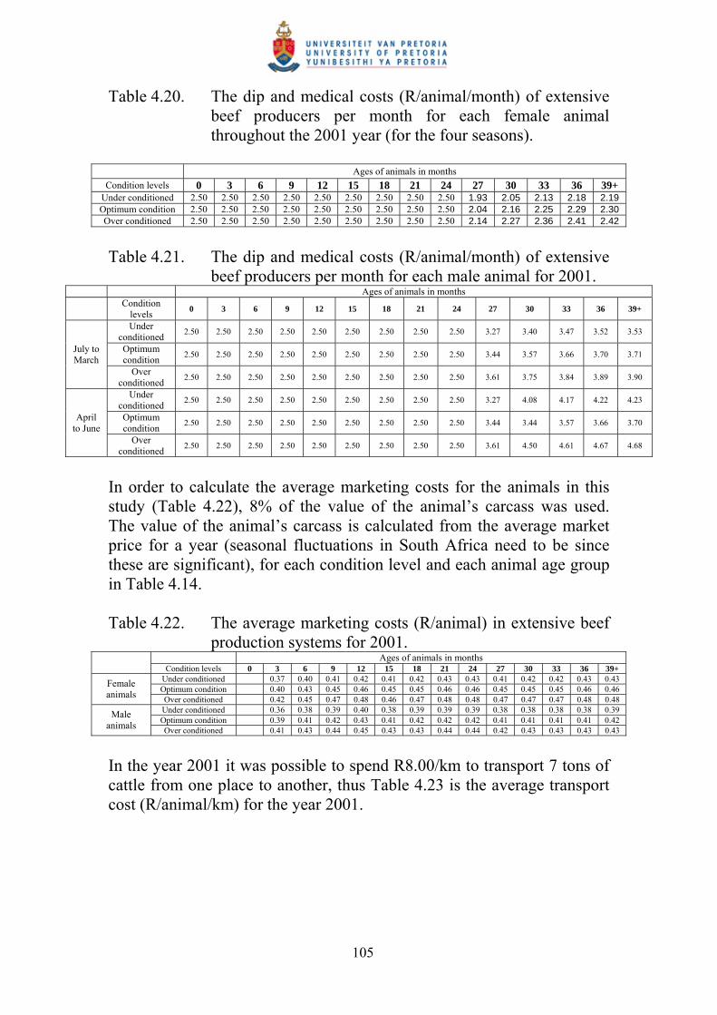
105

Table 4.20. The dip and medical costs (R/animal/month) of extensive beef producers per month for each female animal throughout the 2001 year (for the four seasons).

Ages of animals in months

Condition levels 0 3 6 9 12 15 18 21 24 27 30 33 36 39+ Under conditioned 2.50 2.50 2.50 2.50 2.50 2.50 2.50 2.50 2.50 1.93 2.05 2.13 2.18 2.19 Optimum condition 2.50 2.50 2.50 2.50 2.50 2.50 2.50 2.50 2.50 2.04 2.16 2.25 2.29 2.30 Over conditioned 2.50 2.50 2.50 2.50 2.50 2.50 2.50 2.50 2.50 2.14 2.27 2.36 2.41 2.42

Table 4.21. The dip and medical costs (R/animal/month) of extensive

beef producers per month for each male animal for 2001. Ages of animals in months

Condition

levels 0 3 6 9 12 15 18 21 24 27 30 33 36 39+

Under

conditioned 2.50 2.50 2.50 2.50 2.50 2.50 2.50 2.50 2.50 3.27 3.40 3.47 3.52 3.53

July to March

Optimum condition

2.50 2.50 2.50 2.50 2.50 2.50 2.50 2.50 2.50 3.44 3.57 3.66 3.70 3.71

Over

conditioned 2.50 2.50 2.50 2.50 2.50 2.50 2.50 2.50 2.50 3.61 3.75 3.84 3.89 3.90

Under

conditioned 2.50 2.50 2.50 2.50 2.50 2.50 2.50 2.50 2.50 3.27 4.08 4.17 4.22 4.23

April to June

Optimum condition

2.50 2.50 2.50 2.50 2.50 2.50 2.50 2.50 2.50 3.44 3.44 3.57 3.66 3.70

Over

conditioned 2.50 2.50 2.50 2.50 2.50 2.50 2.50 2.50 2.50 3.61 4.50 4.61 4.67 4.68

In order to calculate the average marketing costs for the animals in this study (Table 4.22), 8% of the value of the animal’s carcass was used. The value of the animal’s carcass is calculated from the average market price for a year (seasonal fluctuations in South Africa need to be since these are significant), for each condition level and each animal age group in Table 4.14. Table 4.22. The average marketing costs (R/animal) in extensive beef

production systems for 2001. Ages of animals in months

Condition levels 0 3 6 9 12 15 18 21 24 27 30 33 36 39+ Under conditioned 0.37 0.40 0.41 0.42 0.41 0.42 0.43 0.43 0.41 0.42 0.42 0.43 0.43 Optimum condition 0.40 0.43 0.45 0.46 0.45 0.45 0.46 0.46 0.45 0.45 0.45 0.46 0.46

Female animals

Over conditioned 0.42 0.45 0.47 0.48 0.46 0.47 0.48 0.48 0.47 0.47 0.47 0.48 0.48 Under conditioned 0.36 0.38 0.39 0.40 0.38 0.39 0.39 0.39 0.38 0.38 0.38 0.38 0.39 Optimum condition 0.39 0.41 0.42 0.43 0.41 0.42 0.42 0.42 0.41 0.41 0.41 0.41 0.42

Male animals Over conditioned 0.41 0.43 0.44 0.45 0.43 0.43 0.44 0.44 0.42 0.43 0.43 0.43 0.43

In the year 2001 it was possible to spend R8.00/km to transport 7 tons of cattle from one place to another, thus Table 4.23 is the average transport cost (R/animal/km) for the year 2001.

106

Table 4.23. The average transport costs (R/animal/km) in extensive beef production systems for 2001.

Ages of animals in months Condition levels 0 3 6 9 12 15 18 21 24 27 30 33 36 39+

Under conditioned 0.03 0.11 0.16 0.19 0.23 0.26 0.29 0.33 0.36 0.39 0.42 0.44 0.44 0.45 Optimum condition 0.03 0.11 0.17 0.20 0.24 0.27 0.31 0.34 0.38 0.42 0.44 0.46 0.47 0.47

Female animals

Over conditioned 0.03 0.12 0.18 0.22 0.25 0.29 0.32 0.36 0.40 0.44 0.46 0.48 0.49 0.49 Under conditioned 0.03 0.11 0.19 0.27 0.37 0.44 0.51 0.58 0.63 0.67 0.69 0.71 0.72 0.72 Optimum condition 0.03 0.12 0.20 0.29 0.39 0.47 0.54 0.61 0.66 0.70 0.73 0.75 0.76 0.76

Male animals Over conditioned 0.03 0.12 0.21 0.30 0.41 0.49 0.56 0.64 0.69 0.74 0.77 0.78 0.79 0.80

All the tables discussed above were incorporated into the cattle farm planning system with the help of linear programming done by Mr W de Boer.

107

CHAPTER 5

RESULTS AND DISCUSSION 5.1 The cattle farm planning system programme

· The programming language The Pilot programme itself was written in Borland/Interplus Delphi. The corresponding database handler, Paradox, was also used.

· The help files There would be two types of help files that may be accessed at all times from the Toolbar icon or the Help icon displayed on various screens in the system. The first type of help file assists in operating the system and the second type assists in understanding the system (what actually appears on the screen). An additional feature is that messages will be ‘spoken’ in a language of choice. This will especially be used to inform the farmer of useful management strategies. 5.1.1 Example of the output from the programme The output from the programme works as follows. First, the marketing strategy is displayed. For each season, the number of cattle recommended for sale is graphically displayed, together with the corresponding gross and net income. The net income equals the sales costs minus marketing and transport costs. By clicking on a specific animal age group, the user may select the marketing strategy for this group, for the coming two years in each of eight seasons. Then the herd composition is displayed together with the financial information. Currently, the programme only provides information on running costs, but in later versions the cash flow and other financial information will also be provided. The data may again be selected for each animal age group separately. The rainfall and temperature icon is important because it determines the protein and crude fibre content of pastures in any particular region (Bonsma, 1980).

108

Step 1

Figure 5.1. The cattle farm planning system computer programme start-

up screen. In order to start the computer programme the farmer must click on the green mark icon on the start up screen (Figure 5.1) of the Cattle Farm Planning System programme. The logon screen will then appear with the available farms. To select a farm, the user must scroll up or down and click on the required farm, the selected farm will appear in green (Figure 5.2).

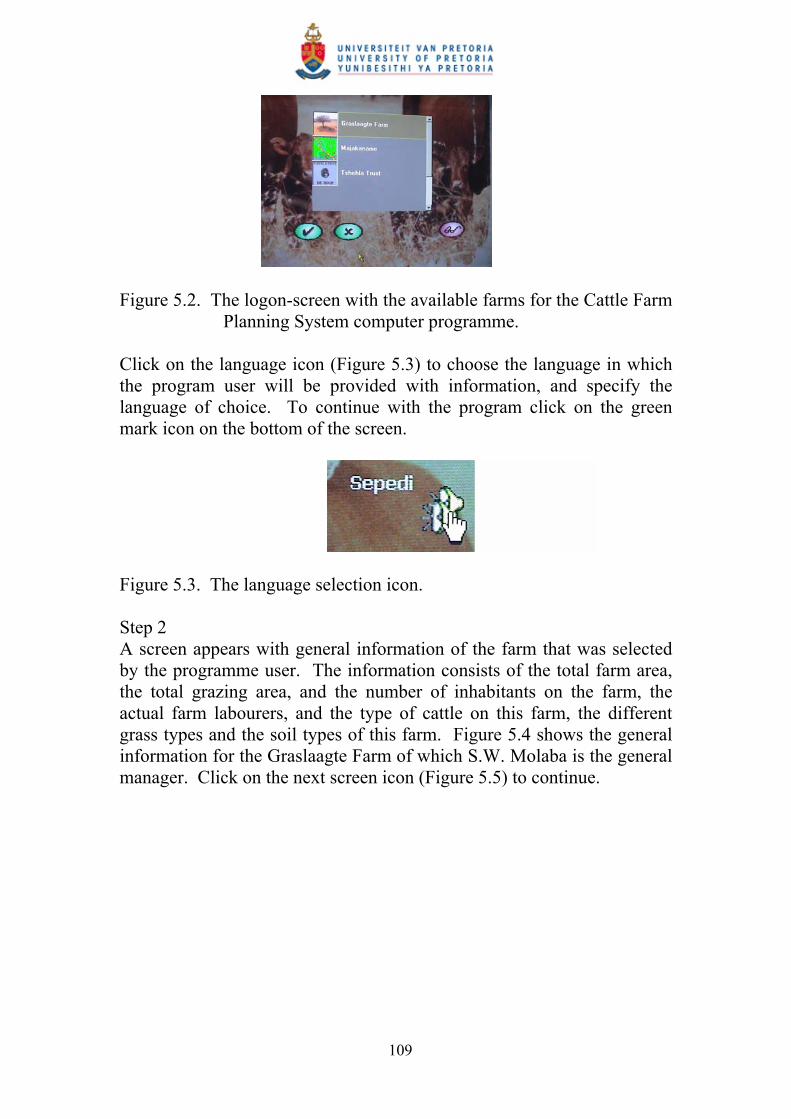
109

Figure 5.2. The logon-screen with the available farms for the Cattle Farm Planning System computer programme.

Click on the language icon (Figure 5.3) to choose the language in which the program user will be provided with information, and specify the language of choice. To continue with the program click on the green mark icon on the bottom of the screen.

Figure 5.3. The language selection icon. Step 2 A screen appears with general information of the farm that was selected by the programme user. The information consists of the total farm area, the total grazing area, and the number of inhabitants on the farm, the actual farm labourers, and the type of cattle on this farm, the different grass types and the soil types of this farm. Figure 5.4 shows the general information for the Graslaagte Farm of which S.W. Molaba is the general manager. Click on the next screen icon (Figure 5.5) to continue.

110

Figure 5.4. General information of the Graslaagte Farm where S.W.

Molaba is the manager.

Figure 5.5. The next screen icon. Step 3 The farmer types the expected rainfall and temperatures for the specific time and specific farm into the table that appears on the screen. Click the save icon and continue. Figure 5.6 shows the output of the rainfall and temperatures for the Majakaname Farm where Geelboy Mailula is the manager.

111

Figure 5.6. The predicted rainfall and temperatures for the Majakaname

Farm of Geelboy Mailula. The icons will show the farmer when it will be dry, which is the case in the picture in the upper right corner, or if there is sufficient grazing, the picture in the bottom left corner. Step 4 To alter the composition of the herd or to make sure that the information on the herd composition is still valid, click on the current herd icon (Figure 5.7).

Figure 5.7. The current herd icon. A screen appears where the current herd composition can be entered. The composition of the herd consists of: the number of calves in the herd; the number of young heifers in the herd; the number of young steers in the herd; the number of young cows in the herd; the number of old cows in the herd and the number of bulls in the herd. Figure 5.8 shows the output entered of the herd composition of the Graslaagte Farm. Click the save icon to continue.

112

Figure 5.8. The current herd composition of the Graslaagte Farm of

which S.W. Molaba is the manager. Step 5 To start the calculation of the cost effectiveness, the farmer must click the large cattle unit icon (Figure 5.9). Values can be added by the farmer to use in the calculation of the cost effectiveness for the specific farm selected. The information that can be altered consists of the dip and medical costs, the cost of licks and concentrate, marketing costs, the costs of transport, the current meat price and the price of the animal on the hoof (Figure 5.10). Other information that also appears on this screen is the percentage dead, dead calves and culling percentages of cows and bulls. All of these can be altered. The information on the animal mass, minimum and maximum feed required and water requirement of the animals must also be entered.

Figure 5.9. The large cattle unit icon.

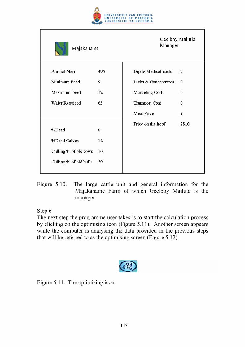
113

Figure 5.10. The large cattle unit and general information for the

Majakaname Farm of which Geelboy Mailula is the manager.

Step 6 The next step the programme user takes is to start the calculation process by clicking on the optimising icon (Figure 5.11). Another screen appears while the computer is analysing the data provided in the previous steps that will be referred to as the optimising screen (Figure 5.12).

Figure 5.11. The optimising icon.

114

Figure 5.12. The optimising screen. The sales and marketing costs are shown on the screen so that the farmer can see what the profit margin will be (Figure 5.13).

Figure 5.13. The sales and marketing cost for all cattle on the Tshehla

Trust Farm where John Tshehla is the manager. Step 7 Using the information in the tables that is described in Section 4.2.2, the system will determine the running cost for all cattle (Figure 5.15) on the specific farm. In order to reach this screen, click on the financial position icon (Figure 5.14).

115

Figure 5.14. The financial position icon.

Figure 5.15. The running cost for all cattle on the Tshehla Trust Farm where John Tshehla is the manager.

Step 8 This is an optional step that works like a help file. This function can be used any time during the whole process. This type of help file will give some helpful tips concerning farming. To enable this feature, the user needs to click on the farming tips icon (Figure 5.16).

Figure 5.16. The farming tips icon. The user will find this a helpful management tool (Figure 5.17). The programme urges the farmer to check daily for sick cattle, inspect the animals’ skins, make sure that the animals are eating and drinking, gives advice on the health of the animals, gives the farmer a indication which

116

cattle to keep in the herd, and which cattle to sell off with reason. And also gives advice on the general improvement of the herd.

Figure 5.17. The help feature for the cattle farm planning system

computer programme.

117

CHAPTER 6

CONCLUSIONS AND RECOMMENDATIONS 6.1 Conclusions Because of the complicated nature of beef cattle farming it was necessary to develop an effective computerised cattle management system, the Cattle Farm Planning System. A mathematical model was developed with the use of data from previous researchers, on growth, fertility, mating and calving percentages and data on the dressing percentages, average producer prices as well as other expenses. Growth curves for animals with three different condition score’s was used in conjunction with the expected meat prices and dressing percentages to calculate the expected market prices on the hoof of the different animals. Sales and marketing costs can be viewed on screen in order to show the farmer his profit margin. Tables were drawn based on the data from previous researchers, and using the information from the tables the system also determined the running costs for all cattle on the specific farm. The output of the program works as follow. First, the marketing strategy will be displayed. For each season the number of cattle recommended for sale will be graphically displayed, together with the corresponding gross and net income. The user can also select the marketing strategy for a specific group of cattle for the coming two years in each of eight seasons. The herd composition can also be displayed with financial information. Farming systems in South Africa differ markedly, and the emerging farmers as well as small-farming communities depend either entirely or partly on agricultural activities for their survival and income generation. The cattle farm planning system (pilot project) that was developed provides a tool whereby a farmer, or farming communities, can manage their farms in an economically viable manner, thus obtaining maximum profit for the user. Most importantly this management tool is provided for different livestock types (major project), production systems and conditions on a site-specific basis, in a user-friendly document-driven software environment. 6.2 Future research focus 6.2.1 Envisaged modelling needs of future versions Future challenges for mechanistic models concern the accurate simulation of feed intake and growth, even in extreme situations for example severe

118

under nutrition (loss of weight) and compensatory growth. These models would also be much more reliable for use in normal situations, and would allow a good prediction of response curves, such as carcass quality (including composition of fatty tissues) and excretion fluxes (nitrogen, minerals, water). Mechanistic mathematical models have contributed greatly to an increased understanding of plant and crop physiology, yet acceptance of the benefits to be gained from similar models of animal digestion and metabolism has been much slower. These models (if properly constructed) can be used to test hypotheses, to aid interpretation, to increase understanding and to improve experimental design (France et al, 1987). However, mechanistic approaches also have serious drawbacks, which could limit their construction, their use and therefore their usefulness. One of the main difficulties when trying to build a mechanistic model is the provision of numerical values for the parameters. The latter are generally numerous in models aimed at integrating aspects of metabolism, and are multiplied with the consideration of individual tissues or organs. A mechanistic model describes underlying phenomena, and some of the required parameter values concern physiological mechanisms. Therefore, aggregative values as commonly found in standard experiments are generally not adequate for parameterisation, even if they can be used during the validation phase. If literature or experiments provide values on a certain number of flows and transactions, the building of a model quite inevitably highlights areas where data is missing and where parameters have to be estimated or extrapolated from other situations or animal species. This is particularly true for models for research purposes. The problem is then to decide what proportion of such uncertain data a model may include. For relatively simple models or sub models, values of parameters can nevertheless be estimated from aggregated results through statistical studies. This kind of drawback, which appears during building and validation of the model, is even worse when the model includes some entities that are either theoretical or not directly produced in the experiments. In the nutrient partitioning models of growth: the animal is defined by its chemical composition, but the entities associated (total body protein, total body fat) are only seldom available in the literature. Therefore, the modeller needs to use some empirical relationships to relate a conceptual entity to a measurable one, which decreases the reliability of the model

119

outputs. For all these reasons, models based on metabolic fates were, until now, less accurate than simple nutrient partitioning models in current situations. However, they are useful as research tools as they can help in the explanation of phenomena. Another limitation to the mechanistic models is the fact that models including more factors of variation making it necessary for the user to enter more input variables. This becomes particularly difficult when these variables are difficult or costly to obtain, or when their practical meaning is not necessarily clear to the user (Bastianelli and Sauvant, 1997). Another problem is that models are based on data collected at specific sites; consequently the conclusions are relevant only for the animals raised on the specific sites. Differences in the quality of veld and management may affect the reliability of specific models for other farms. The system is also only practical if the farmer receives some assistance (Meyer, 1993). Research results are used by a limited group of farmers. The most important reason for the limited adoption of research results in the developing countries is that the vast majority of farmers have no access to the new technologies proposed by research (Arnon, 1981). This model aims to rectify the situation and, with some further development could provide an easy method of assessing profitability and utilisation of resources for systems on a specific farm. Providing alternative performance indicators to allow farmers and their advisors to reach management decisions, based on their own preferred criteria, is an integral and important feature of the model. Initial findings indicate that there is reasonable correspondence between suggested and actual practice, but wider and more rigorous testing needs to be carried out (Cameron and Wilson, 1996). Thus the beef model would have to be validated in different beef production systems in order to determine its accuracy or usefulness. The model is not necessarily immediately relevant in all production systems but an important contribution thereof is that it assists greatly in identifying deficiencies within production systems. There are also two very important criteria that must be considered when comparing future options, and these are cash flow and stocking pressure (or density) (Gillard and Monypenny, 1987).

120

6.3 Critical evaluation My critical evaluation of this thesis and the work contained therein is: Developing the Cattle Farm Planning System is a complex task. This study could not have been done without the help of the experts in the various fields such as programming, for instance. This project gave me the opportunity to be exposed to disciplines in which I had no formal training, especially software development. The challenge for the 21st century is to find successful ways of using land and other natural resources, for livestock production to create wealth, by increasing efficiency and minimising the use of non-renewable resources, and to do so without compromising environmental quality and the quality of human life. Thus producing food, which is safe and of high quality, in a sustainable manner. In setting objectives for the future within this conceptual framework, there is a continuing need to increase our knowledge, and understanding, of the biophysical processes which control and determine the efficiency of livestock systems, and to take advantage of the clean technologies that will be developed within the next decade. It is however, clear that there is an urgent need to incorporate this knowledge and understanding, and the technological opportunities arising from them, into explicit and logical management aids and tools for livestock farmers and advisors. The development of decision support tools and systems requires research on the most useful way by which biophysical and economic models can be integrated in the design of interactive decision support software. It is imperative that the end-user of the decision support system participates fully in its design, since it is only by doing so that the system will have any chance of being useful. The ultimate goal must be to design support systems that aid effective communication and understanding, and improve the predictability of the outcomes of decision-making (Maxwell, 1996), this study gave the scientific foundations for the development of a decision support tool but in order to provide a accurate prediction model intensive experiments still need to be done. I believe that the Cattle Farm Planning System provides a tool, which in the final instance, can and will increase the effectiveness of farm utilisation. This system is still only a managerial tool and thus is not a replacement for bad management. The Cattle Farm Planning System’s design and modelling was focused on providing usable answers, whilst at the same time not attempting to over-simplify something which is

121

unavoidably complex. As a result, I conclude that the research investigations and research outputs contained in this thesis add value to the field of knowledge regarding animal science and extensive beef production.

122

References References

ARC, 1980. Agricultural research council. The nutrient requirements of ruminant livestock. Commonw. Agric. Bur., Slough. ARNON, I., 1981. Modernization of agriculture in developing countries: Resources, potentials and problems. In: Environmental monographs and symposia. A series in the environmental sciences. Ed. N. Polunin. John Wiley & Sons Ltd. Chichester. AZZAM, S.M., KINDER, J.E. & NIELSEN, M.K., 1990. Modelling reproductive management systems for cattle. Agric. Syst. 34: 103 – 122. BASTIANELLI, D. & SAUVANT, D., 1997. Modelling the mechanisms of pig growth. Livestock Prod. Sci. 51: 97 – 107. BASTIMAN, B. & PULLAR, D., 1996. Methods for transferring research findings into farming practice: development of a successful suckled beef system. In: Livestock farming systems. Research, development, socio-economics and the land manager. Proceedings of the third international symposium on livestock farming systems. EAAP Publication no 79. Ed. J.B. Dent, M.J. McGregor and A.R. Sibbald. Wageningen Pers, Wageningen Pers, The Netherlands. BELTRÁN, J.J., BUTTS, W.T., OLSON, T.A. & KOGER, M., 1992. Growth patterns of two lines of Angus cattle selected using predicted growth parameters. J. Anim. Sci. 70: 734 – 741. BERKEY, C. S., 1982. Bayesian approach for a nonlinear growth model. Biometrics. 38: 953 – 961. BLACK, J.L., 1974. Manipulation of body composition through nutrition. Proc. Aust. Soc. Anim. Prod. 10: 211 – 218. BLACK, J.L., 1983. Growth and development of lambs. In: Sheep production. Ed. W. Haresign. Butterworths, London. BLACK, J.L. & GRIFFITHS, D.A., 1975. Effects of live weight and energy intake on nitrogen balance and total N requirement of lambs. Br. J. Nutr. 33: 339 – 413.

123

BONSMA, J., 1980. Livestock production. A global approach. Tafelberg Publishers Ltd, Cape Town. South Africa. BOSMAN, D.J., 1997. National beef cattle performance and progeny testing scheme (1993 - 1997). Livestock Improvement Schemes, Irene, South Africa. BOSMAN, H.G., AYANTUNDE, A.A., STEENSTRA, F.A. & UDO, H.M.J., 1997. Simulation model to assess productivity of goat production in the tropics. Agric. Syst. 54: 539 – 576. BOSTON, R.C., FOX, D.G., SNIFFEN, C., JANCZEWSKI, E., MUNSON, R. & CHALUPA, W., 2000. The conversion of a scientific model describing dairy cow nutrition and production to an industry tool: the CPM dairy project. In: Modelling nutrient utilization in farm animals. Ed. J.P. McNamara, J. France and E.E. Beever. CABI Publishing. Wallington, UK. BRAKER, M.J.E., 2001. The analysis of subsistence farming systems and the influence of commercialisation of goats on these systems in South Africa. MSc thesis. University of Pretoria, Pretoria. BRODY, S., 1945. Bioenergetics and growth. Rheinhold publishing, New York. BROWN, J.E., FITZHUGH, H.A. & CARTWRIGHT, T.C., 1976. A comparison of nonlinear models for describing weight-age relationships in cattle. J. Anim. Sci. 42: 810 – 818. BRYDEN, M.M., EVANS, H.E. & BINNS, W., 1972. Embryology of the sheep. I. Extra embryonic membranes and the development of body form. J. Morph. 138: 169 – 186. BUTLER FLORA, C. & FRANCIS, C., 1999. Farming systems extension in the USA. FSR in extension and policy formulation. In: A history of farming systems research. Ed. M. Collinson. CABI publishing, a division of CAB international. CALARCO, P.G. & McLAREN, A., 1976. Ultra structural observations of preimplantation stages of the sheep. J. Embryol. Exp. Morph. 36: 609 – 622.

124

CAMERON, R.F. & WILSON, R.M., 1996. A beef system selection model for advisors. In: Livestock farming systems. Research, development, socio-economics and the land manager. Proceedings of the third international symposium on livestock farming systems. EAAP Publication no 79. Ed. J.B. Dent, M.J. McGregor and A.R. Sibbald. Wageningen Pers, Wageningen Pers, The Netherlands. CHENOST, M. & PRESTON, T.R., 1992. Improving cattle growth and finishing in the tropics. In: World animal science, C5. Beef cattle production. Ed. R. Jarrige and C. Béranger. Elsevier Science publishers B.V. Amsterdam, The Netherlands. CLEMEN, R.T., 1996. Making hard decisions. An introduction to decision analysis. 2nd edition. Duxbury press. An imprint of Brooks/Cole publishing company. Johannesburg. COLLINSON, M., 1999a. Editorial introduction. Institutional commitment to farming systems research. In: A history of farming systems research. Ed. M. Collinson. CABI publishing, a division of CAB international. COLLINSON, M., 1999b. My FSR origins. FSR: origins and perspectives. In: A history of farming systems research. Ed. M. Collinson. CABI publishing, a division of CAB international. COOPER, M. McG. & WILLIS, M.B., 1989. Profitable beef production. Farming Press Ltd. Princes Street, United Kingdom. CRICHTON, J.S., 1992. Bull management. In: Beef in Natal. Natal region of the Agricultural Development. Pietermaritzburg, South Africa. CURLL, M.L., DAVIDSON, J.L. & FREER, M., 1975. Efficiency of lamb production in relation to the weight of the ewe at mating and during pregnancy. Aust. J. Agric. Res. 26: 553 – 565. DeNISE, R.S.K. & BRINKS, J.S., 1985. Genetic and environmental aspects of the growth curve parameters in beef cows. J. Anim. Sci. 61: 1431 – 1440.

125

DEPARTMENT OF AGRICULTURAL TECHNICAL SERVICES. 1965. Beef cattle farming in the Transvaal bushveld. Compiled by officials of the Transvaal region, the division of veterinary field services and the department of agricultural economics and marketing. Government printer, Pretoria. South Africa. DU PREEZ, J.J., JARVIS, M.J.F., CAPATOS, D. & DE KOCK, J., 1992. A note on growth curves for the ostrich (Struthio camelus). Anim. Prod. 54: 150 – 152. DIXON, J., 1999. A farming systems contribution to agricultural policy analysis. FSR in extension and policy formulation. In: A history of farming systems research. Ed. M. Collinson. CABI publishing, a division of CAB international. DOREN, P.E. & BAKER, J.F., 1989. Estimating parameters of growth curves of bulls. J. Anim. Sci. 67:1432 – 1445. DREW, K.R. & REID, J.T., 1975. Compensatory growth in immature sheep. III. Feed utilization by sheep subjected to feed deprivation followed by realimentation. J. Agric. Sci., Camb. 85: 215 – 220. DUCKHAM, A.N. & MASEFIELD, G.B., 1971. Farming systems of the world. Chatto & Windus Ltd. London. ESCOBAR, G., 1999. My initiation into FSR in Latin America. FSR: origins and perspectives. In: A history of farming systems research. Ed. M. Collinson. CABI publishing, a division of CAB international. EVERITT, G.C., 1964. Maternal under nutrition and retarded foetal development in merino sheep. Nature. 201: 1341 – 1342.

FARRINGTON, J., 1999. The development of diagnostic methods in FSR. FSR – understanding farming systems. In: A history of farming systems research. Ed. M. Collinson. CABI publishing, a division of CAB international. FITZHUGH, H.A., 1976. Analysis of growth curves and strategies for altering their shape. J. Anim. Sci. 42: 1036 – 1051.

126

FOWLER, V.R., 1980. Growth in mammals for meat production. In: Studies in the agricultural and food sciences: Growth in animals. Ed. T.L.J. Lawrence. Butterworth & Co (South Africa)(Pty) Ltd, Durban, South Africa. FRANCE, J., GILL, M., THORNLEY, J.H.M. & ENGLAND, P., 1987. A model of nutrient utilization and body composition in beef cattle. Anim. Prod. 44: 371 – 385. GAMMON, D.M., 1992a. Making the most of veldt grazing. In: Beef in Natal. Natal region of the Agricultural Development. Pietermaritzburg, South Africa. GAMMON, D.M., 1992b. On-animal performance recording. In: Beef in Natal. Natal region of the Agricultural Development. Pietermaritzburg, South Africa. GARCÍA-MUÑIZ, J.G., HOLMES, C.W., GARRICK, D.J., LÓPEZ-VILLALOBOS, N., WICKHAM, B.W., WILSON, G.F., BROOKES, I.M. & PURCHAS, R.W., 1998. Growth curves and productivity of Holstein-Friesian cows bred for heavy or light mature live weight. Proc. New Zealand Soc. Anim. Prod. 58: 68 – 72. GAROIAN, L., 1981. A dynamic linear programming model applicable to range cattle operations. University Microfilms International. A Bell & Howell Information Company. Ann Arbor, Michigan. GERHARDY, H., 1997. Integration of livestock farming systems into beef marketing systems. In: Livestock farming systems. More than food production. Proceedings of the fourth international symposium on livestock farming systems. EAAP Publication. Wageningen Pers, Wageningen, The Netherlands. GIBON, A., RUBINO, R., SIBBALD, A.R., SØRENSEN, J.T., FLAMANT, J.C., LHOSTE, P. & REVILLA, R., 1996. A review of current approaches to livestock farming systems in Europe: towards a common understanding. In: Livestock farming systems. Research, development, socio-economics and the land manager. Proceedings of the third international symposium on livestock farming systems. EAAP Publication no 79. Ed. J.B. Dent, M.J. McGregor and A.R. Sibbald. Wageningen Pers, Wageningen Pers, The Netherlands.

127

GILLARD, P. & MONYPENNY, R., 1987. A decision support approach for the beef cattle industry of tropical Australia. Agric. Sys. 26: 179 – 190. GRAHAM, N.M., BLACK, J.L., FAICHNEY, G.J. & ARNOLD, G.W., 1976. Simulation of growth and production in sheep-model 1: A computer programme to estimate energy and nitrogen utilisation, body composition and empty live weight change, day by day for sheep of any age. Agric. Syst. 1: 113 – 138. GRAHAM, N.M. & SEARLE, T.W., 1979. Studies of weaned lambs before, during and after a period of weight loss. I. Energy and nitrogen utilization. Aust. J. Agric. Res. 30: 513 – 523. GREEFF, J.C., SCHOLTZ, M.M. & ROUX, C.Z., 1993. Preliminary genetic parameters of growth during different growth phases in sheep. S. Afr. J. Anim. Sci. 23: 57 – 60. HAMMOND, J., 1955. Progress in the physiology of farm animals. Volume 2. Butterworth Scientific publications, London. HUNTER, G.L., 1957. The maternal influence on size in sheep. J. Agric. Sci. Cambridge. 48: 36 – 60. JACOBS, G.A., 1992a. Energy supplements for beef cattle on veld and pastures. In: Beef in Natal. Natal region of the Agricultural Development, Pietermaritzburg, South Africa. JACOBS, G.A., 1992b. Principles of winter feeding and supplementary feeding during winter (winter licks). In: Beef in Natal. Natal region of the Agricultural Development, Pietermaritzburg, South Africa. JACOBS, G.A., 1992c. Mineral licks for summer. In: Beef in Natal. Natal region of the Agricultural Development, Pietermaritzburg, South Africa. JARRIGE, R., & AURIOL, P., 1992. An outline of world beef production. In: World animal science C. Production-system approach 5. Beef cattle production. Ed. R. Jarrige & C. Béranger. Elsevier Science Publishers. The Netherlands.

128

JASIOROWSKI, H.A., 1976. The developing world as a source of beef for world markets. In: Beef cattle production in developing countries. Proceedings of the conference held in Edinburgh from the 1st to 6th September 1974 organized by the centre for tropical veterinary medicine. Ed. A.J. Smith. University of Edinburgh Centre for Tropical Veterinary Medicine. Lewis Reprints Ltd, Tonbridge. JOLICOEUR, P. & HEUSNER, A.A., 1986. Log-normal variation belts for growth curves. Biometrics. 42: 785 – 794. JOSHI, N.R., McLAUGHLIN, E.A. & PHILLIPS, R.W., 1957. Types and breeds of African cattle. Food and agriculture organization of the United States. Rome. Italy. KAPS, M., HERRING, W.O. & LAMBERSON, W.R., 1999. Genetic and environmental parameters for mature weight in Angus cattle. J. Anim. Sci. 77:569 – 574. KEEN, P.G.W. & SCOTT MORTON, M.S., 1978. Decision support systems: An organizational perspective. Addison-Wesley publishing company, Inc. Don Mills, Ontario. KEMPSTER, A.J., 1992. Carcass characteristics and quality. In: World animal science C. Production-system approach 5. Beef cattle production. Ed. R. Jarrige & C. Béranger. Elsevier Science Publishers. The Netherlands. KREINER, H.A., 1990. Studies of growth and efficiencies of bulls and steers of the Bovelder and bulls of the Drakensberger, Bonsmara and Brahman cattle breeds. LADEMAN, E.E., 1975. Kudde bestuur. Mara Navorsingstasie, Die Vleisnywerheid, Okt-Des. LASTER, D.B., SMITH, G.M. & GREGORY, K.E., 1976. Characterization of biological types of cattle. IV. Postweaning growth and puberty of heifers. J. Anim. Sci. 43: 63 – 70. LOUW, B.P., 1992. Pasture finishing. In: Beef in Natal. Natal region of the Agricultural Development. Pietermaritzburg, South Africa.

129

LOUW, B.P., BARTHOLOMEW, P.E. & PATERSON, A.G., 1992. The beef breeding herd on pastures. In: Beef in Natal. Natal region of the Agricultural Development. Pietermaritzburg, South Africa.

LOUW, B.P. & LISHMAN, A.W., 1992. Breeding seasons. In: Beef in Natal. Natal region of the Agricultural Development. Pietermaritzburg, South Africa. MATATA, J.B.W., ANANDAJAYASEKARAM, P, KIRIRO, T.N., DIXON, J. & WANDERA, E.O., undated. Farming systems approach to technology development and transfer. Kida. Farmesa, Sida . Kenya, Uganda, Tanzania, Zambia and Zimbabwe. Unpublished report. MAXWELL, T.J., 1996. Conclusions of the symposium. Where do we go from here? In: Livestock farming systems. Research, development, socio-economics and the land manager. Proceedings of the third international symposium on livestock farming systems. EAAP Publication no 79. Ed. J.B. Dent, M.J. McGregor and A.R. Sibbald. Wageningen Pers, Wageningen Pers, The Netherlands. McCURLEY, J.R., BUTTS, W.T., KOGER, M. & PAHNISH, O.F., 1980. Utilization of early growth performance and body measurements to predict mature weight and rate of maturing in beef cattle. J. Anim. Sci. 51: 30(suppl. 1). MEAKER, H.J., 1984. Effective extensive beef production. Meat Board Focus, Sept-Oct. p 15-19. MENCHACA, M.A., CHASE, C.C., OLSON, T.A. & HAMMOND, A.C., 1996. Evaluation of growth curves of Brahman cattle of various frame sizes. J. Anim. Sci. 74: 2140 – 2151. MEYER, D.H., 1993. Modelling in support of decision-making for South African extensive beef farmers. Orion. 9: 37 – 54. MEYER, K., 1999. Estimates of genetic phenotypic covariance functions for postweaning growth and mature weight of beef cows. J. Anim. Breed. Genet. 116: 181 – 205. MEYER, K., 1995. Estimates of genetic parameters for mature weight of Australian beef cows and its relationship to early growth and skeletal measures. Livestock Prod. Sci. 44: 125 – 137.

130

MORROW, R.E., McLAREN, J.B. & BUTTS, W.T., 1978. Effect of age on estimates of bovine growth-curve parameters. J. Anim. Sci. 47: 352 – 357. MURRAY, D.M. & SLEZACEK, O., 1975. The effect of growth rate on muscle distribution in sheep. J. Agric. Sci., Camb. 85: 189 – 191. NADARAJAH, K., MARLOWE, T.J. & NOTTER, D.R., 1984. Growth

patterns of Angus, Charolais, Charolais×Angus and Holstein×Angus

cows from birth to maturity. J. Anim. Sci. 59: 957 – 966. NEEDHAM, A.E., 1964. The growth process in animals. Sir Isaac Pitman & Sons Ltd. The Pitman Press, Bath, Great Britain. NORMAN, D., 1999. FSR: a personal evolution. FSR: origins and perspectives. In: A history of farming systems research. Ed. M. Collinson. CABI publishing, a division of CAB international. NORMAN, D.W., 1993. The farming systems perspective: The key to building sustainable agriculture in Southern Africa. In: The proceedings of the Southern African association for farming systems research-extension conference 1993. Hosted by the FSR-E Swaziland Conference Committee. NRC, 1984. Nutrient requirements of beef cattle. National Academy Press. Washington, D.C. NRC, 1996. Nutrient requirements of beef cattle, seventh revised edition. National Academy Press. Washington, D.C. NVNS, 1983. Nasionale vleisbees prestasie en nageslagtoets skema. Nuusbrief 37 (Julie). OLTJEN, J.W., PLEASANTS, A.B., SOBOLEVA, T.K. & ODDY, V.H., 2000. Second-generation dynamic cattle growth and composition models. In: Modelling nutrient utilization in farm animals. Ed. J.P. McNamara, J. France and E.E. Beever. CABI Publishing. Wallington, UK.

131

ØRSKOV, E.R., McDONALD, I., GRUBB, D.A. & PENNIE, K., 1976. The nutrition of the early weaned lamb. IV. Effects on growth rate, food utilization and body composition of changing from a low to a high protein diet. J. Agric. Sci., Camb. 86: 411 – 423. OWENS, F.N. & GEAY, Y., 1992. Nutrition of growing and finishing cattle. In: World animal science C. Production-system approach 5. Beef cattle production. Ed. R. Jarrige & C. Béranger. Elsevier Science Publishers. The Netherlands. PALMER, M.J., PHILLIPS, B.F. & SMITH, G.T., 1991. Application of nonlinear models with random coefficients to growth data. Biometrics. 47: 623 – 633. PATERSON, A.G., 1992. The practical selection and culling of cows, replacement heifers and bulls. In: Beef in Natal. Natal region of the Agricultural Development. Pietermaritzburg, South Africa. PEROTTO, D., CUE, R.I. & LEE, A.J., 1992. Comparison of nonlinear functions for describing the growth curve of three genotypes of dairy cattle. Can. J. Anim. Sci. 72: 733 – 782. PETIT, M., JARRIGE, R., RUSSEL, A.J.F. & WRIGHT, I.A., 1992. Feeding and nutrition of the suckler cow. In: World animal science C. Production-system approach 5. Beef cattle production. Ed. R. Jarrige & C. Béranger. Elsevier Science Publishers. The Netherlands. PETERS, A.R. & BALL, P.J.H., 1987. Reproduction in cattle. Butterworth & Co. Ltd. London. POMEROY, R.W., 1955. Live-weight growth. In: Progress in the physiology of farm animals. Volume 2. Ed. J. Hammond. Butterworths Scientific Publications, London. PRESCOTT, J.H.D., 1976. Growth and development of beef cattle. In: Beef cattle production in developing countries. Proceedings of the conference held in Edinburgh from the 1st to 6th September 1974 organized by the centre for tropical veterinary medicine. Ed. A.J. Smith. University of Edinburgh Centre for Tropical Veterinary Medicine. Lewis Reprints Ltd, Tonbridge. PRESTON, T.R. & WILLIS, M.B., 1970. Intensive beef production. Pregamon Press. Great Britain.

132

PROVOST, A. & UILENBERG, G., 1992. Diseases as a limiting factor. In: World animal science C. Production-system approach 5. Beef cattle production. Ed. R. Jarrige & C. Béranger. Elsevier Science Publishers. The Netherlands. RENAND, G., PLASSE, D. & ANDERSEN, B.B., 1992. Genetic improvement of cattle growth and carcass traits. In: World animal science C. Production-system approach 5. Beef cattle production. Ed. R. Jarrige & C. Béranger. Elsevier Science Publishers. The Netherlands. REVELL, B.J. & CRABTREE, J.R., 1996. Policy pressures and responses in European livestock systems. In: Livestock farming systems. Research, development, socio-economics and the land manager. Proceedings of the third international symposium on livestock farming systems. EAAP Publication no 79. Ed. J.B. Dent, M.J. McGregor and A.R. Sibbald. Wageningen Pers, Wageningen Pers, The Netherlands. ROBELIN, J. & TULLOH, N.M., 1992. Patterns of growth of cattle. In: World animal science C. Production-system approach 5. Beef cattle production. Ed. R. Jarrige & C. Béranger. Elsevier Science Publishers. The Netherlands. RUSSEL, A.J.F., FOOT, J.Z., WHITE, I.R. & DAVIES, G.J., 1981. The effect of weight at mating and of nutrition during mid-pregnancy on the birth weight of lambs from primiparous ewes. J. Agric. Sci., Camb. 97: 723 – 729. SAMIC. South African Meat Industry Company. PO Box 36802 Menlopark 0102. South Africa. SAUVANT, D., 1996. Use of systems modelling in animal nutrition linked to livestock farming systems. In: Livestock farming systems. Research, development, socio-economics and the land manager. Proceedings of the third international symposium on livestock farming systems. EAAP Publication no 79. Ed. J.B. Dent, M.J. McGregor and A.R. Sibbald. Wageningen Pers, Wageningen Pers, The Netherlands. SEARLE, T.W., GRAHAM, N.M. & SMITH, E., 1979. Studies of weaned lambs before, during and after a period of weight loss. II. Body composition. Aust. J. Agric. Res. 30: 525 – 531.

133

SEARLE, T.W. & GRIFFITHS, D.A., 1976. The body composition of growing sheep during milk feeding, and the effect on composition of weaning at various body weights. J. Agric. Sci., Camb. 86: 483 – 493. SERAGELDIN, I., 2001. Changing agendas for agricultural research. In: Agricultural science policy. Changing global agendas. Ed. J.M. Alston, P.G. Pardey & M.J. Taylor. John Hopkins university press. Baltimore, Maryland. SHORT, B.F., 1955. Developmental modification of fleece structure by adverse maternal nutrition. Aust. J. Agric. Res. 6: 863 – 872. SØRENSEN, J.T., 1997. Conclusions from the symposium. In: Livestock farming systems. More than food production. Proceedings of the fourth international symposium on livestock farming systems. EAAP Publication. Wageningen Pers, Wageningen, The Netherlands. SØRENSEN, J.T. & HINDHEDE, J., 1997. On-farm experiments as a research method in animal welfare and health. In: Livestock farming systems. More than food production. Proceedings of the fourth international symposium on livestock farming systems. EAAP Publication. Wageningen Pers, Wageningen, The Netherlands. SQUIRES, V.R. & VERA, R.R., 1992. Commercial beef ranching in tropical and semi-arid zones. In: World animal science, C5. Beef cattle production. Ed. R. Jarrige and C. Béranger. Elsevier Science publishers B.V. Amsterdam, The Netherlands. THIMONIER, J. & SIGNORET, 1992. Reproduction of the beef herd. In: World animal science, C5. Beef cattle production. Ed. R. Jarrige and C. Béranger. Elsevier Science publishers B.V. Amsterdam, The Netherlands. THOMPSON, J.M., ATKINS, K.D. & GILMOUR, A.R., 1979. Carcass characteristics of heavyweight crossbred lambs. II. Carcass composition and partitioning of fat. Aust. J. Agric. Res. 30: 1207 – 1214. TOULLEC, R., 1992. Veal production. In: World animal science, C5. Beef cattle production. Ed. R. Jarrige and C. Béranger. Elsevier Science publishers B.V. Amsterdam, The Netherlands. UDO, H. & CORNELISSEN, T., 1998. Livestock in resource-poor farming systems. Outlook on Agriculture. 27: 237 – 242.

134

VAN NIEKERK, A. & LISHMAN, A.W., 1992. Selection and rearing of replacement heifers. In: Beef in Natal. Natal region of the Agricultural Development. Pietermaritzburg, South Africa. VAN NIEKERK, B.D.H., 1975. Supplementation of grazing cattle. Proceedings: Seminar on potential to increase beef production in tropical America. CIAT. Cali, Columbia, p 83-94. WALKER, D.M. & NORTON, B.W., 1971. The utilization of the metabolizable energy of diets of different protein content by the milk-fed lamb. J. Agric. Sci., Camb. 77: 363 – 369. WALLACE, L.R., 1948a. The growth of lambs before and after birth in relation to the level of nutrition. Part I. J. Agric. Sci., Camb. 38: 93 – 153. WALLACE, L.R., 1948b. The growth of lambs before and after birth in relation to the level of nutrition. Part II and III. J. Agric. Sci., Camb. 38: 243 – 302. WALLACE, L.R., 1948c. The growth of lambs before and after birth in relation to the level of nutrition. Part III. J. Agric. Sci., Camb. 38: 367 – 401. WIDDOWSON, E.M., 1980. Definitions of growth. In: Growth in animals. Ed. T.L.J. Lawrence. Butterworths, London. WINCHESTER C.F. & MORRIS, M.J., 1956. Water intake rates of cattle. J. Anim. Sci. 15: 722 – 740.