Embed Size (px)
Citation preview

MODELLING ELECTRICITY SPOT PRICE TIME
SERIES USING COLOURED NOISE FORCES
By
Adeline Peter Mtunya
A Dissertation Submitted in Partial Fulfilment of the Requirements
for the Degree of Master of Science (Mathematical Modelling) of
the University of Dar es Salaam
University Of Dar es Salaam
May, 2010

i
CERTIFICATION
The undersigned certify that they have read and hereby recommend for accep-
tance by the University of Dare es Salaam a dissertation entitled: Modelling
Electricity Spot Price Time Series Using Coloured Noise Forces, in
partial fulfillment of the requirements for the degree of Master of Science (Math-
ematical modelling) of the University of Dar es Salaam.
Prof. T. Kauranne
(First Supervisor)
Date: ...........................................
Dr. W. C. Mahera
(Second supervisor)
Date: ...........................................

ii
DECLARATION AND COPYRIGHT
I, Adeline Peter Mtunya, declare that this dissertation is my own original
work and that it has not been presented and will not be presented to any other
University for a similar or any other degree award.
Signature:
This dissertation is copyright material protected under the Berne Convention,
the Copyright Act 1999 and other international and national enactments, in that
behalf, on intellectual property. It may not be reproduced by any means, in
full or in part, except for short extracts in fair dealings, for research or private
study, critical scholarly review or discourse with an acknowledgement, without
the written permission of the Directorate of Postgraduate Studies, on behalf of
both the author and the University of Dar es Salaam.

iii
ACKNOWLEDGEMENTS
I would like to express my sincere gratitude to my supervisors, Prof. Tuomo
Kauranne (Lappeenranta University of Technology) and Dr. W. C. Mahera (Uni-
versity of Dar es Salaam) for their constant support, guidance and constructive
ideas throughout my research work. I have learned so much from them about
stochastic modelling and its application to time series and finance.
Special thanks goes to Heads of Mathematics Department of my time of study,
Dr. A. R. Mushi and Dr. E. S. Massawe, who made all efforts to provide me
with a conducive study environment. I wish to express my sincere appreciation
to all staff members in the Department of Mathematics for their support and
encouragement. I extend my thanks to Deputy Principal (Academics), Mkwawa
University College of Education (MUCE) for the sponsorship that enabled me
to undertake this study. Also many thanks to NORAD’s programme for Master
Studies (NOMA) who sponsored the whole Mathematical modelling program.
I would like to thank Lappeenranta University of Technology (LUT) - Finland,
for providing me admission under exchange program for the whole period of
preparing my dissertation for nine months. It was great opportunity for me to
meet different experties in the field of my research and other close related fields. I
wish to thank CIMO (Center for International Mobility) for providing scholarship
for the whole period of my stay at LUT.
Warmest thanks to my fellow master’s students in the Department of Mathe-
matics. Their cooperative spirit and contribution during the whole period of my
study is appreciated.
Last but not least, I would like to express my utmost thanks to my parents,
brothers and sisters for their love and encouragement during the whole period of
my study.

iv
DEDICATION
To my lovely parents Peter Mtunya and Adela Tarimo

v
ABSTRACT
In this dissertation we develop a mean-reverting stochastic model driven by
coloured noise processes for modelling electricity spot price time series. The
deregulation of electricity market, which once believed to be natural monopoly,
has led to the creation of power exchanges where electricity is traded like other
commodities. The physical attributes of electricity and behaviour of electricity
prices differ from other commodity market. Electricity spot prices in the emerging
power markets experience high volatility, mean-reversion, spikes and seasonal pat-
terns mainly due to non-storability nature of electricity. Uncontrolled exposure
to market price risks can lead to devastating consequences for market partici-
pants in the restructured electricity industry. A precise statistical (econometric)
model of electricity spot price behaviour is necessary for risk management, pricing
of electricity-related options and evaluation of production assets. We therefore
formulate and discuss the stochastic approach used to model the spot prices of
electricity by coloured noise forces. Parameter estimation for the model is car-
ried out by Maximum Likelihood Estimation (MLE) method on mean-reverting
stochastic process. Data used for model calibration were collected from Nord Pool
for the period starting from January, 1999 to February, 2009. With the estimated
parameters we simulate the model and found that the simulated and real price
series have similar trends and covers the same price ranges. Thus, modelling of
electricity spot prices using coloured noise gives a good approximation to real
prices and we recommend application of coloured noise when modelling the spot
prices of electricity.

vi
Contents
Certification . . . . . . . . . . . . . . . . . . . . . . . . . . . . . . . . . i
Declaration and Copyright . . . . . . . . . . . . . . . . . . . . . . . . . ii
Acknowledgements . . . . . . . . . . . . . . . . . . . . . . . . . . . . . iii
Dedication . . . . . . . . . . . . . . . . . . . . . . . . . . . . . . . . . . iv
Abstract . . . . . . . . . . . . . . . . . . . . . . . . . . . . . . . . . . . v
Table of Contents . . . . . . . . . . . . . . . . . . . . . . . . . . . . . . vi
List of Figures . . . . . . . . . . . . . . . . . . . . . . . . . . . . . . . . x
List of Tables . . . . . . . . . . . . . . . . . . . . . . . . . . . . . . . . xii
List of Abbreviations . . . . . . . . . . . . . . . . . . . . . . . . . . . . xiii
CHAPTER ONE: INTRODUCTION 1
1.1 General Introduction . . . . . . . . . . . . . . . . . . . . . . . . . 1
1.2 Economic Terminologies in pricing of electricity: . . . . . . . . . . 4
1.2.1 Power exchange. . . . . . . . . . . . . . . . . . . . . . . . 4
1.2.2 Demand and Supply. . . . . . . . . . . . . . . . . . . . . . 5
1.2.3 Wholesale and Retail markets. . . . . . . . . . . . . . . . . 6
1.2.4 Energy derivatives. . . . . . . . . . . . . . . . . . . . . . . 7
1.2.5 Options. . . . . . . . . . . . . . . . . . . . . . . . . . . . . 8

vii
1.2.6 Complete and Incomplete markets. . . . . . . . . . . . . . 9
1.2.7 Over The Counter (OTC) Markets. . . . . . . . . . . . . . 9
1.3 Electricity trading in Nordic countries. . . . . . . . . . . . . . . . 10
1.4 Electricity behaviour. . . . . . . . . . . . . . . . . . . . . . . . . . 12
1.4.1 Special features of electricity. . . . . . . . . . . . . . . . . 13
1.4.2 Stylized features of Electricity Spot Prices. . . . . . . . . . 14
1.5 Current state of electricity trade in Tanzania . . . . . . . . . . . . 17
1.5.1 Electricity generation . . . . . . . . . . . . . . . . . . . . . 17
1.5.2 Electricity Transmission and Distribution . . . . . . . . . . 18
1.5.3 Electricity selling . . . . . . . . . . . . . . . . . . . . . . . 19
1.6 Mathematical terms in stochastic modelling. . . . . . . . . . . . . 20
1.7 Statement of the Problem . . . . . . . . . . . . . . . . . . . . . . 21
1.8 Reseach Objectives . . . . . . . . . . . . . . . . . . . . . . . . . . 22
1.8.1 General Objectives . . . . . . . . . . . . . . . . . . . . . . 22
1.8.2 Specific Objectives . . . . . . . . . . . . . . . . . . . . . . 22
1.9 Significance of the Study . . . . . . . . . . . . . . . . . . . . . . . 23
CHAPTER TWO: LITERATURE REVIEW 24
CHAPTER THREE: PRICE MODEL BY COLOURED NOISE 31

viii
3.1 Introduction . . . . . . . . . . . . . . . . . . . . . . . . . . . . . . 31
3.2 Model development: . . . . . . . . . . . . . . . . . . . . . . . . . . 31
3.3 Mathematical Description of Coloured Noise Process: . . . . . . . 33
3.4 Parameter estimation . . . . . . . . . . . . . . . . . . . . . . . . . 35
3.4.1 Maximum Likelihood Estimation(MLE) of Mean Reverting
Process: . . . . . . . . . . . . . . . . . . . . . . . . . . . . 36
CHAPTER FOUR: DATA ANALYSIS AND METHODOLOGY 43
4.1 Source of Data . . . . . . . . . . . . . . . . . . . . . . . . . . . . 43
4.2 Statistical Analysis of the Data . . . . . . . . . . . . . . . . . . . 43
4.2.1 Data Description . . . . . . . . . . . . . . . . . . . . . . . 43
4.2.2 Normality test . . . . . . . . . . . . . . . . . . . . . . . . . 46
4.2.3 Serial correlation in the return series . . . . . . . . . . . . 50
4.3 Calibration of the model. . . . . . . . . . . . . . . . . . . . . . . . 52
4.4 Analysis of Coloured Noise used in Simulation . . . . . . . . . . . 54
4.5 Model simulation, results and comparison . . . . . . . . . . . . . . 57
4.6 Application on Pure trading . . . . . . . . . . . . . . . . . . . . . 60
4.7 Forward price . . . . . . . . . . . . . . . . . . . . . . . . . . . . . 62
CHAPTER FIVE: CONCLUSION AND RECOMMENDATIONS 66
4.1 Conclusion. . . . . . . . . . . . . . . . . . . . . . . . . . . . . . . 66

ix
4.2 Recommendations and Future work. . . . . . . . . . . . . . . . . . 67

x
List of Figures
1 Deregulation allows competition in generation and selling leaving
transmission and distribution monopolistic. . . . . . . . . . . . . . 2
2 An increase in demand (from D1 to D2) resulting in an increase in
price (P) and quantity (Q) sold of the product. . . . . . . . . . . 6
3 Determination of price from Supply and Demand curves. . . . . . 11
4 Electricity production in Nordic countries - 2007. . . . . . . . . . 12
5 Daily average electricity spot price since 1st January, 1999 until
28th April, 2009 (3712 observations). . . . . . . . . . . . . . . . . 45
6 The logarithm of electricity prices from which the main features of
electricity market are observed. . . . . . . . . . . . . . . . . . . . 45
7 Normal probability test for electricity prices returns. . . . . . . . 47
8 Histogram showing distribution of price returns superimposed with
a theoretical normal curve. . . . . . . . . . . . . . . . . . . . . . . 48
9 Histogram for logarithm of spot prices showing distribution of log-
prices for the data, superimposed with the theoretical normal curve. 49
10 Log-returns price series showing the existence of some price spikes. 49
11 ACF for price return series showing some important lags. Where
most of the values fall out of the bounds. Seasonality can be ob-
served from the lags with strong 7 - day dependence. . . . . . . . 51
xi
12 PACF for price return series, where some values are out of the
bounds. . . . . . . . . . . . . . . . . . . . . . . . . . . . . . . . . 51
13 The original log-prices, the trend and the detrended data. . . . . 53
14 The logarithm of electricity spot prices with removed spikes. . . . 53
15 The noise processes: (a)white noise ξ(t), (b)coloured noise filtered
once ζ1(t) and (c)coloured noise filtered twice ζ2(t) . . . . . . . . 55
16 The white noise ξ(t) and coloured noise filtered twice ζ2(t) which
is applied in an SDE for modelling the spot log-prices. . . . . . . 55
17 An increase in correlation observed after plotting noise levels against
their previous values due to filtering of white noise. . . . . . . . . 56
18 An increase in correlation observed from the Sample Autocorrela-
tion Function (ACF) due to filtering of white noise. Stationarity
of the coloured noise is also clear from the lags. . . . . . . . . . . 56
19 Simulation results for logarithm of Prices vs real (original) log-prices. 58
20 Simulated Electricity Spot Prices Time-series versus Real Prices. 58
21 Distribution of the original electricity spot prices (a) and the sim-
ulated electricity prices (b). . . . . . . . . . . . . . . . . . . . . . 59
22 Histogram of the residuals. . . . . . . . . . . . . . . . . . . . . . . 59
23 Pure price series since 1st January, 1999 until 28th April, 2009. . 61
24 Simulated vs real (original) pure price series. . . . . . . . . . . . . 61

xii
List of Tables
1 Descriptive statistics for the daily average electricity spot prices. . 44
2 Daily electricity log-prices parameter estimates for the model. . . 53
3 Real (original) spot prices data vs Simulated data. . . . . . . . . . 60
4 Real (original) pure-prices data vs Simulated data. . . . . . . . . 62

xiii
ABBREVIATIONS
ACF Auto-correlation Function
AR AutoRegressive
ARMA AutoRegressive Moving Average
ATM Automated Teller Machine
EEX European Power Exchange (Power-exchange in Germany)
GARCH Generalized AutoRegressive Conditionally Heteroskedastic
GBM Geometric Brownian Motion
IPP Independent Power Producers/Projects/Plants
IPTL Independent Power Tanzania Ltd
MRS Markov Regime Switching
OTC Over The Counter markets
PACF Partial Autocorrelation Function
SADC Southern African Development Community
SDE Stochastic Differential Equation

CHAPTER ONE
INTRODUCTION
1.1 General Introduction
The electricity sector has long been an integral part of the engine of economic
growth and a central component of sustainable development. During the 1990s,
conventional wisdom about the electricity sector was turned on its head. Pre-
viously, electricity had been considered a natural monopoly, and the electricity
sector in most countries was either owned or strictly regulated by the government.
Particularly in developing countries, government leadership in the development
and use of electricity was a part of a broader ‘social compact’. Then, with as-
tonishing speed, a revolution in thinking swept the sector. Several countries
undertook major reforms, ranging from opening their electricity markets to in-
dependent power generators to broad-based reforms remaking the entire sector
around the objective of promoting competition. Due in part to these changes,
$187 billion was invested in energy and electricity projects in developing coun-
tries and the economies in transition in Central and Eastern Europe between 1990
and 1999. A 1998 survey of 115 developing countries found that nearly two thirds
had taken at least minimal steps toward market-oriented reforms in the electric-
ity sector [2]. In Tanzania for instance, electricity market is not yet deregulated.
There is only one public owned company that is in charge of electricity business –
TANESCO. However the deregulation of electricity seems to be right on the way
to its starting point as there are a few companies that produce electricity but at
the moment must sell it to TANESCO.
Analysis of the electricity industry begins with the recognition that there are four
rather distinct activities of it: generation, selling (trading), transmission and dis-
tribution. Deregulation has in most cases allowed competition in generation and
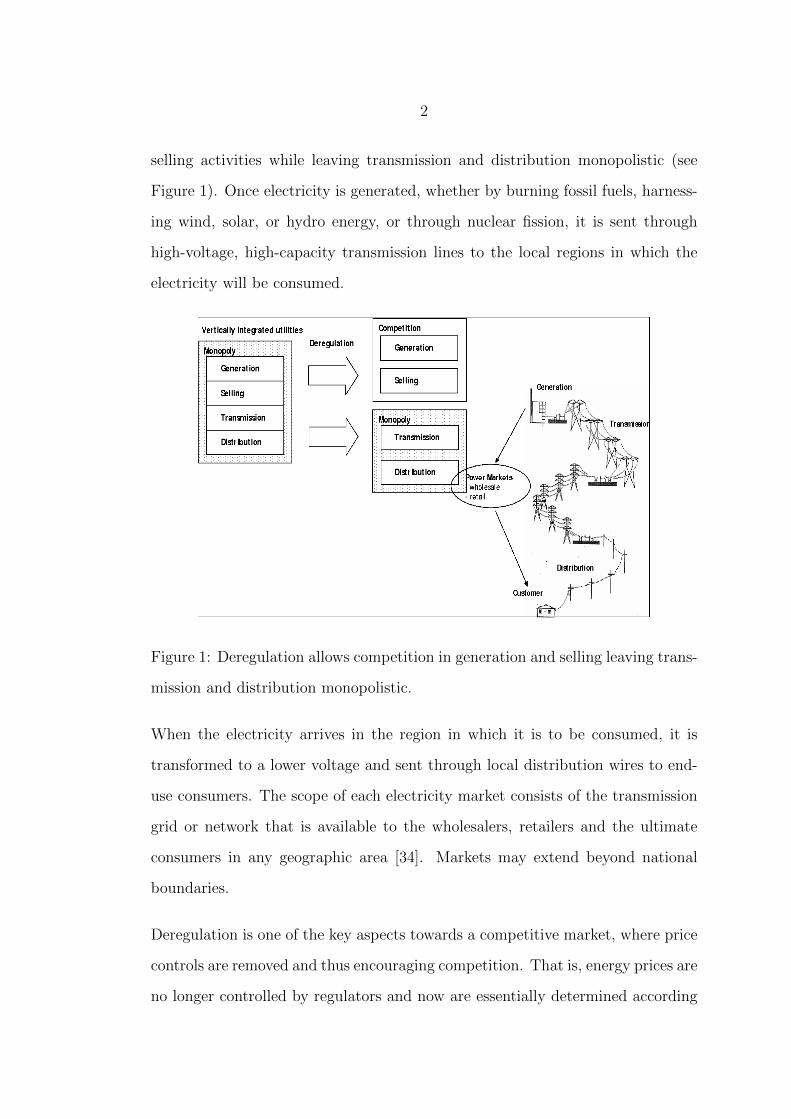
2
selling activities while leaving transmission and distribution monopolistic (see
Figure 1). Once electricity is generated, whether by burning fossil fuels, harness-
ing wind, solar, or hydro energy, or through nuclear fission, it is sent through
high-voltage, high-capacity transmission lines to the local regions in which the
electricity will be consumed.
Figure 1: Deregulation allows competition in generation and selling leaving trans-
mission and distribution monopolistic.
When the electricity arrives in the region in which it is to be consumed, it is
transformed to a lower voltage and sent through local distribution wires to end-
use consumers. The scope of each electricity market consists of the transmission
grid or network that is available to the wholesalers, retailers and the ultimate
consumers in any geographic area [34]. Markets may extend beyond national
boundaries.
Deregulation is one of the key aspects towards a competitive market, where price
controls are removed and thus encouraging competition. That is, energy prices are
no longer controlled by regulators and now are essentially determined according

3
to the economic rule of supply and demand. The earliest introduction of energy
market concepts and privatization to electric power systems took place in Chile in
the early 1980s. However the oldest electricity market is Nord Pool that started
in 1991 for the trading of all hydro electric power generated by Norway. The
daily spot market has been operational since May 1999 and in 2001 a total of
8.24 TWh were traded on this market. Nord Pool benefited from the fact that
electricity in Scandinavia is in great part hydroelectricity, hence has the very
valuable property of being storable. The non storability of the other forms of
electricity is an important explanatory factor of the spikes as those which were
observed in the United States in the ECAR market in June 1998 [15]. Today,
the Nord Pool is a successful exchange, where the electricity players in Europe
feel they can place their orders safely. Apart from Nord Pool, some other major
European electricity exchanges include: UK Power Exchange (UKPX) – England
(2001), OMEL – Spain (1998), Amsterdam Power Exchange (APX) – Netherlands
(1999), European Power Exchange (EEX) – Germany (2001) and Polish Power
Exchange - Poland (2000). These had been governed by EU legislation directives
in 1996 and 2003. European goal was to have fully competitive electricity markets
in all EU Member States by 1st of July 2007, and eventually to have common
European electricity market [34].
Provision of reliable and cost-effective electricity sources in the rural communi-
ties of developing countries (such as Tanzania) for the achievement of social and
economic empowerment and poverty alleviation is imperative within the context
of the global millennium development goals (MDGs) [29]. Restructuring of the
electricity industry will encourage the availability of reliable and cost-effective
power supply in view of the following conditions which will manifest: Removal of
monopoly in power generation, transmission and distribution and the encourage-
ment of competition in power delivery, Reliability in power delivery, Lower energy
tariffs, Increasing the scope for choice, Incorporation of more energy technologies
4
into the energy supply mix.
Electricity markets differ from the traditional financial markets and other com-
modity markets due to the non-storability, uncertain and inelastic demand, re-
strictive transportation networks and a steep supply curve. And these are the
reasons behind high volatility of electricity spot prices. Supply and demand must
be in balance at each instance separately. A viable model for the spot price
process is of up-most importance in all the areas of deregulated power business,
including derivative and sales pricing, risk analysis, portfolio management, in-
vestment analysis, and regulatory policy making [33]. The market risk related
to trading is considerable due to extreme volatility of electricity prices. This is
especially true for spot prices, where the volatility can be as high as 50% on the
daily scale, which is over ten times higher than for other energy products (natural
gas and crude oil) [36]. In this research we aim at studying the techniques for
pricing of electric energy derivatives.
In this chapter we explain some terminologies used in pricing, discuss electricity
trading in Nordic counties and the behaviour of electricity. We then assess the
current state of electricity trade in Tanzania. Also, together with mathematical
terms in stochastic modelling, we include the statement of the problem, research
objectives and significance of the study. Chapter two is on literature review while
chapter three presents the price model in details. Chapter four is on data analysis
and methodology and in chapter five we give the conclusion.
1.2 Economic Terminologies in pricing of electricity:
1.2.1 Power exchange.
The Power Exchange is an entity responsible for receiving bids for sales and
purchases of electricity, and to match the bids in such a way that prices and

5
quantities are settled [34]. The basic activity of the power exchange is operation
of the short term physical electricity market, the spot market. A power exchange
is an open, centralized, and neutral market place, where the market price of
electricity is determined by demand and supply. A high liquidity ensures that
the market price at the power exchange is a ‘correct’ price. The products sold at
the exchange are standard products, and the communication is equitable to all
actors on the market. The operation of the power exchange is market-oriented, in
other words, the members of the power exchange participate in decision making.
Therefore it is possible to make the product structure of the power exchange meet
the needs of the market participants.
1.2.2 Demand and Supply.
In economics, demand is the desire to own anything and the ability to pay for it
and willingness to pay. The term demand signifies the ability or the willingness
to buy a particular commodity at a given point of time. Demand is also defined
elsewhere as a measure of preferences that is weighted by income. Economists
record demand on a demand schedule and plot it on a graph as an inverse down-
ward sloping curve. The inverse curve reflects the relationship between price and
demand: as demand increases, price increases as shown in Figure 2.

6
Figure 2: An increase in demand (from D1 to D2) resulting in an increase in price
(P) and quantity (Q) sold of the product.
Supply on the other hand represents the amount of goods that producers are
willing and able to sell at various prices, assuming all determinants of supply
other than the price of the good in question, such as technology and the prices
of factors of production, remain the same. Under the assumption of perfect
competition, supply is determined by marginal cost. Marginal cost is the change
in total cost that arises when the quantity produced changes by one unit. Firms
will produce additional output as long as the cost of producing an extra unit of
output is less than the price they will receive.
1.2.3 Wholesale and Retail markets.
A wholesale electricity market exists when competing generators offer their elec-
tricity output to retailers. The retailers then re-price the electricity and take it

7
to market, in a classic example of the middle man scenario. While wholesale pric-
ing used to be the exclusive domain of the large retail suppliers, more and more
markets like New England are beginning to open up to the end users. Large end
users seeking to cut out unnecessary overhead in their energy costs are beginning
to recognize the advantages inherent in such a purchasing move. Buying direct
is certainly not a novel concept in economics, however it is relatively novel in the
electricity context.
A retail electricity market exists when end-use customers can choose their supplier
from competing electricity retailers. A separate issue for electricity markets is
whether or not consumers face real-time pricing (prices based on the variable
wholesale price) or a price that is set in some other way, such as average annual
costs. In many markets, consumers do not pay based on the real-time price, and
hence have no incentive to reduce demand at times of high (wholesale) prices
or to shift their demand to other periods. Demand response may use pricing
mechanisms or technical solutions to reduce peak demand. Generally, electricity
retail reform follows from electricity wholesale reform. However, it is possible to
have a single electricity generation company and still have retail competition.
1.2.4 Energy derivatives.
An energy derivative is a financial contract whose value depends on energy price.
The emergence of the energy markets has given birth to energy derivative mar-
kets. For example, a forward contract is an obligation to buy or sell electricity
for a predetermined price at a predetermined future time [12]. By definition, a
derivative security is a security whose price depends on or is derived from one or
more underlying assets. An option is one example of many derivative securities
found in the market. The derivative itself is a contract between two or more par-
ties. Its value is determined by the price fluctuations of the underlying asset. The

8
most common underlying assets include: stocks, bonds, commodities, currencies,
interest rates and market indexes. Two of the most widely used such derivative
securities are the futures contracts and the forward contracts. In futures contract,
the settlement of the net value is started immediately after making the contract,
and it is carried out daily until the end of the delivery time. A forward is a
contract in which delivery of the underlying commodity is referred at a later date
than when the contract is written with the price of delivery being set at the time
of contracting.
1.2.5 Options.
An option is a contract between a buyer and a seller that gives the buyer the
right, but not the obligation, to buy or to sell a particular asset (the underlying
asset) on or before the option’s expiration time, at an agreed price, the strike
price. An option contract binds only the seller (also called writer) of the option.
In return for granting the option, the seller collects a payment (the premium)
from the buyer as a compensation for the risk taken. Two types of options exist
in the market. A call option gives the buyer the right to buy the underlying asset
and a put option gives the buyer of the option the right to sell the underlying
asset. If the buyer chooses to exercise this right, the seller is obliged to sell or buy
the asset at the agreed price. The buyer may choose not to exercise the right and
let it expire. The underlying asset can be a piece of property, a security (stock
or bond), or a derivative instrument, such as a futures contract. The theoretical
value of an option is evaluated according to several models. These models attempt
to predict how the value of an option changes in response to changing conditions.
Hence, the risks associated with granting, owning, or trading options may be
quantified and managed with a greater degree of precision.

9
1.2.6 Complete and Incomplete markets.
A market is complete with respect to a trading strategy if there exists a self-
financing trading strategy such that at any time t, the returns of the two strategies
are equal. In general, a complete market is a market in which every derivative
security can be replicated by trading in the underlying asset or assets. That means
a market must be possible to instantaneously enter into any position regarding
any future state of the market.
An incomplete market is the one missing the above property. At any given time at
the stock market, the stock price can increase or decrease slightly or fall a lot. It is
not possible to hedge against all these increase or decrease in price simultaneously
because there is no opportunity to carry out a continuous changing delta hedge,
this leads to impossibility of perfect hedging. The impossibility of perfect hedging
means that the market is incomplete, that is not every option can be replicated
by a self-financing portfolio. It is not early to mention that a power exchange is
an incomplete market.
1.2.7 Over The Counter (OTC) Markets.
In finance, Over-the-counter (OTC) or off-exchange trading is to trade financial
instruments such as commodities or derivatives directly between two parties in
contrast with exchange trading. Exchange trading occurs via facilities constructed
for the purpose of trading (i.e., exchanges), such as futures exchanges or stock
exchanges. OTC markets refer to all wholesale trade in electricity outside power
exchange. With the services provided by the OTC markets, it is possible for the
actors on the market to tailor their portfolios of purchase and sale contracts to
accurately meet their needs. Unlike in the trading at the power exchange, there is
a risk of a counterparty default. The power exchange and the OTC markets that
complement each other together form a well-functioning market mechanism for

10
the wholesale of electricity, the objective of which is to control the high volatility
of the electricity market prices.
1.3 Electricity trading in Nordic countries.
All Nordic countries have liberalised their electricity markets. The electricity
markets in the Nordic countries have undergone major changes since the middle
of the 1990s. The purpose of the liberalisation was to create better conditions for
competition, and thus to improve utilisation of production resources as well as
to provide gains from improved efficiency in the operation of networks. Norway
was the first Nordic country to launch the liberalisation process of its electricity
market with the approval of the Energy Act in 1990, which introduced regulated
third-party access. Norway was followed by Sweden and Finland in the middle
of the 1990s and by Denmark at the beginning of 1998 when the large electricity
customers were given access to the electricity network. The liberalisation process
in the middle of the 1990s was followed by an integration of the Nordic mar-
kets. The establishment of Nord Pool, the Nordic electricity exchange, was an
important part of this integration [27].
The physical market is the basis for all electricity trading in the Nordic market.
The spot price set here forms the basis for the financial market. Nord Pool
Spot organises the market place which comprises the Elspot and Elbas products.
Elspot is the common Nordic day ahead market for trading physical electricity
contracts. Elbas is a physical balance adjustment market operating 24 hours
time. Elbas is an intraday market which opens two hours after the spot market
is done and is open until 1 hour before delivery hour. The Nord pool financial
market (Eltermin) provides a market place where the exchange members can trade
derivative contracts in the financial market. Financial electricity contracts are
used to guarantee prices and manage risk when trading power. Nord Pool offers

11
contracts of up to six years’ duration, with contracts for days, weeks, months,
quarters and years.
In Elspot, a trading day is divided into 24 hourly markets. Market participants
provide separate bids for these 24 hours and the market clears separately for each
of these 24 hours. Each participant provides a piece-wise linear bid schedule,
where quantity is measured in MW and price in ¿/MWh by 12 noon for delivery
the following day.
Nord Pool determines the clearing price for each market by 2:00 p.m. at which
time the market closes and final clearing prices are determined. All contracts
become binding at this point and Nord Pool initiates settlement of these contracts.
The bids from each of the participants provide a schedule of how much the bidder
is prepared to sell or buy at different prices. The system price is determined by
the market equilibrium ,i.e, the point where supply and demand curves cross.
Supply willingness to generate electricity at a given price depends on the nature
of production as shown in Figure 3.
Figure 3: Determination of price from Supply and Demand curves.

12
Generally, if there are no transmission constraints, the Nord Pool area is a com-
bined market and market participants can buy or sell electricity at the same price
anywhere in the area. If the system operator designates zones, Nord Pool arranges
separate Elspot markets for each zone. Nord Pool first calculates a theoretical
unconstrained price based on all submitted bids, without considering transmis-
sion constraints. If transmission constraints are binding, Nord Pool adjusts prices
upwards in deficit areas and downwards in surplus areas until transmission con-
straints are satisfied. It is noted that the quantity and nature of electricity pro-
duced varies within Nordic countries, from what is observed in the map shown in
Figure 4.
Figure 4: Electricity production in Nordic countries - 2007.
1.4 Electricity behaviour.
The behaviour of electricity can be explained in two ways. On one side is the
behaviour of electricity as energy (also called load), that is, the physical attributes
of the commodity we are dealing with in the market. On the other side is the

13
behaviour of electricity prices when we value it in the market.
1.4.1 Special features of electricity.
Wangensteen [34] asserts that electricity has certain features that make it a rather
unique commodity. This must be taken into account in power system economics.
The following list captures the essentials:
Continuous flow.
Electricity is generated and consumed in a continuous manner. Gas transported
through a gas grid has basically the same feature.
Instant generation and consumption.
Electricity is consumed in the same moment of time as it is generated. If we
again compare with gas, the transport speed of gas in a pipe is about one meter
per second. Electricity travels with the speed of light.
Non-storability.
Electricity cannot be stored in significant quantities in an economic manner.
Only indirect storage can be realized through hydroelectric plants or storage of
generator fuel. Non-storability is the most significant element that contribute to
the high volatility of electricity prices.
Consumption variability.
Electricity consumption or demand is variable with a characteristic pattern over
day and night, over the week, and over the year. The variability in consumption
is one of the root-causes of the seasonality in prices.
Non-traceability.
There is no physical means by which a unit of electricity (a kWh) delivered to a
consumer can be traced back to the producer that actually generated the unit.

14
This feature puts special requirements on the metering and billing system for
electricity.
Essentiality to the community.
Electricity is regarded as an absolute necessity in a modern society. Practically,
every household and every firm has a connection to the power grid (this refers
particularly to Nordic countries). How essential electricity is can be illustrated
by the Value of Lost Load (VOLL), which is sometimes estimated to 100 times
more than the ordinary price.
Breakdown possibility.
Due to technical characteristics of a power supply system, not only individual
consumers can be affected by a contingency. Large areas can be affected in the
case of a complete system breakdown. We have seen some large breakdowns, for
instance in New York in 1977 and 2003, with tremendous economic consequences.
1.4.2 Stylized features of Electricity Spot Prices.
Electricity spot markets exhibit a number of typical features that are not found
in most financial markets. The most important of those features are:
Seasonality:-
Electricity spot prices reveal seasonal behavior in annual, weekly and daily cycles.
Both the demand side and supply side play part in the seasonality of the spot
prices. Business activities and weather conditions are considered to be the major
factors that are behind the seasonality of electricity prices. It is well known
that electricity demand exhibits seasonal fluctuations. They mostly arise due to
changing climatic conditions, like temperature and the number of daylight hours.
In some countries also the supply side shows seasonal variations in output. Hydro
units, for example, are heavily dependent on precipitation and snow melting,

15
which varies from season to season. These seasonal fluctuations in demand and
supply translate into the seasonal behavior of spot electricity prices. In Nordic
countries for example, the cold winter experiences higher electricity prices and
spikes while prices usually settle down during summer. In some places this is
different [23], Northern California’s primary electricity consumption occurs during
the summer when air conditioning is highly needed.
Volatility:-
Extremely high volatility is experienced in electricity prices. The market risk
related to trading is considerable due to extreme volatility of electricity prices.
This is especially true for spot prices, where the volatility can be as high as 50% on
the daily scale, i.e. over ten times higher than for other energy products (natural
gas and crude oil). The high volatility pattern is due to the transmission and
storage problems and, of course, the requirement of the market to set equilibrium
prices in real time. It is not easy to correct provisional imbalances of supply and
demand in the short-term. Therefore, the price changes are more extreme in the
electricity markets than other financial or commodity ones. With the application
of the standard concept of volatility, the standard deviation of the returns on a
daily scale, Weron [36] obtains the following volatility estimations:
- notes and treasury bills: less than 0.5%
- stock indices: 1 - 1.5%
- commodities like natural gas or crude oil: 1.5 - 4%
- very volatile stocks: not more than 4%
- and electricity up to 50%
Spikes:-
A fundamental property of electricity spot prices, already observed by many

16
authors, is the presence of spikes, that is, rapid upward price moves followed
by a quick return to about the same level. During the peak period, the price
process has different properties. In particular, the rate of mean reversion is much
higher than during normal evolution. The presence of spikes is a fundamental
feature of electricity prices due to the non-storable nature of this commodity and
any relevant spot price model must take this feature into account. The presence
of long-term stochastic variation in the mean level of electricity prices makes it
difficult to establish a range of prices, for which the price process is in peak mode.
What is considered as a peak level now may become normal in 3 years. The rate
of mean reversion is therefore determined not only by the current price level but
also by the previous evolution of the price, which suggests that the behavior of
electricity spot prices may be non-markovian [26].
The occurrence of spikes in power prices dynamics can be understood if we con-
sider that electricity is a very special commodity. With the exception of hydro-
electric power, it cannot be stored and must be generated at the instant it is
consumed; the demand is highly inelastic. The generation process (supply) is
characterized by low marginal costs but, when emergency generators are to be
put on operation in order to satisfy the demand, marginal costs may be very
high. Prices are therefore very sensitive to the demand, to outages and grid
congestions. Thus shortages in electricity generation, forced outages, peaks in
electricity demand determine spikes.
Mean reversion:-
Energy spot prices are in general regarded to be mean-reverting or anti-persistent
[35]. Mean reversion is the tendency of a stochastic process to return over time
to a long-run average value. The speed of mean reversion depends on several
factors, including the commodity itself being analyzed and the delivery provisions
associated with the commodity. When the price of a commodity is high, its supply

17
tends to increase thus putting a downward pressure on the price; when the spot
price is low, the supply of the commodity tends to decrease, thus providing an
upward lift to the price. Thus, in a long run prices will move towards the level
dictated by the cost of production. Moreover Weron[35] mentioned that among
all financial time series spot electricity prices are perhaps the best example of
anti-persistent data.
1.5 Current state of electricity trade in Tanzania
We noted down earlier that electricity business in Tanzania is not yet deregu-
lated, though there are some indications for that to take place in the near future.
Tanzania Electricity Supply Company (TANESCO) is the only fully authorized
for electricity business in the country. TANESCO is wholly owned by the govern-
ment of Tanzania and is under the Ministry of Energy and Minerals. However,
there are some other companies with partial share in the business; these are the
independent power projects (IPPs).
1.5.1 Electricity generation
TANESCO remains the main power producer in the country. Other sources of
generation are from independent power producers (IPPs) which feed the National
grid and isolated areas as well. TANESCO’s generation system consists mainly
of Hydro and Thermal based generation. Hydro contributes the largest share
of TANESCO’s power generation. The total generation from TANESCO own
sources in 2008 was 2,985,275,264kWh out of which 2,648,911,352kWh (90%) was
from Hydro Power Plants [31]. Total country demand was 4,425,403,157kWh, of
which 33% was supplied by IPPs. The hydro-plants operated by TANESCO are
all interconnected with the national grid system.
TANESCO has been implementing power generation mix program, whereby a

18
substantial amount of generation comes from thermal generation through own
generation and independent power plants (IPPs). Own thermal generation comes
from the Ubungo 100MW gas-fired plant in Dar es Salaam. Another 45MW gas-
fired power plant located at Tegeta in Dar es Salaam is expected to enter the grid
system soon.
By the end of year 2008 IPPs contributed a total installed capacity of 282MW.
IPPs powering the national grid include the Independent Power Tanzania Ltd
(IPTL) with 100MW (diesel based) installed capacity and SONGAS (Songo Songo
gas – to electricity project) which by the end of 2007 had 182MW capacity.
TANESCO also imports a total of 10MW of electric power from Uganda and
about 3MW from Zambia.
There are also several diesel generating stations connected to the national grid
with installed capacity of 80MW but the only operational grid diesel based station
is Dodoma which contributes about 5MW. Some other regions, districts and
townships are dependent on isolated diesel-based generators with a total installed
capacity of 31MW. Mtwara and Lindi regions are supplied by M/S Artumas
Group Ltd, an IPP based in Mtwara. The total capacity of Artumas power plant
is 8MW using gas from Mnazi Bay gas wells.
1.5.2 Electricity Transmission and Distribution
Transmission and distribution system is totally owned by TANESCO. Transmis-
sion system comprises of 36 grid substations interconnected by transmission lines.
The transmission lines comprise of 2,732.36km of system voltages 220kV; 1537km
of 132kV; and 534km of 66kV, totaling to 4803.36km by the end of September,
2009. The system is all alternating current (AC) and the system frequency is
50Hz.

19
The Distribution System Network Supply Voltage are 33kV and 11kV which serve
as the back bone stepped down by distribution transformers to 400/230 volts for
residential, light commercial and light industrial supply. There are big commercial
and heavy industries supplied directly at 33kV and 11kV. Distribution activities
are the most intensive in terms of geographical coverage. There are more than
672, 759 customers linked by these distribution lines [31].
1.5.3 Electricity selling
This is also done by TANESCO, since it receives electricity from the other com-
panies through the main grid. The metering system for TANESCO customers are
of two types. First one is Pre-paid Metering System (LUKU): LUKU is a Swahili
abbreviation for “LIPA UMEME KADIRI UNAVYOTUMIA” which means ”pay
for electricity as you use it” and the second type is Credit meters (conventional
meters): These meters allow for customers to be billed after consuming electric-
ity for a month. LUKU has been designed mainly for residential and commercial
consumers, not industrial type. TANESCO uses different tariff rates to differ-
ent customers groups depending on the quantity of electricity consumed. These
include domestic, small business and industrial consumers. The LUKU system
has improved customer services further as now the customers can even buy elec-
tricity online through mobile phones and bank ATMs. For example a customer
can recharge LUKU via ZAP LUKU recharge if is a ZAIN subscriber or M-PESA
LUKU recharge if is a VODACOM subscriber. Recharging LUKU through bank
ATMs can be done for customers who own bank account in CRDB or NMB banks.
In addition to all those businesses, TANESCO actively cooperates with various
Governments and other Power Utility bodies. The major areas of cooperation
include Southern African Power Pool (SAPP), Nile Basin Regional Power Trade
Project and Nile Equatorial Lakes- Subsidiary Action Program (NELSAP).
20
1.6 Mathematical terms in stochastic modelling.
In this section we define some mathematical terms that are to be used in modeling
in this work.
Definition 1 Stochastic process
A stochastic process is a family of random variables X(t, ω) of two variables
t ∈ T, ω ∈ Ω on a common probability space (Ω,F , P ) which assumes real values
and is P -measurable as a function of ω for a fixed t. The parameter t is interpreted
as time, with T being a time interval and X(t, ·) represents a random variable on
the above probability space Ω, while X(·, ω) is called a sample path or trajectory
of the stochastic process. The stock prices and electricity prices are good examples
of stochastic processes.
Definition 2 Stochastic differential equation (SDE)
A stochastic differential equation (SDE) is a differential equation in which one
or more of the terms is a stochastic process, thus resulting in a solution which is
itself a stochastic process. SDEs incorporate white noise which is a derivative of
Brownian motion (Wiener Process); however, other types of random fluctuations
are possible, such as jump processes or coloured noise.
A typical equation is of the form
dXt = µ(Xt, t)dt+ σ(Xt, t)dBt
where µ is the drift function, σ is diffusion function and Bt is the standard
Brownian motion.
Definition 3 Ornstein–Uhlenbeck process
The Ornstein–Uhlenbeck process is a stochastic process rt given by the following
stochastic differential equation:
drt = θ(µ− rt)dt+ σdBt

21
It represents the mean-reverting process with the equilibrium or mean-value µ,
diffusion constant σ and a mean-reversion rate θ. Ornstein–Uhlenbeck process is a
Gaussian process that has a bounded variance and admits a stationary probability
distribution used to model (with modifications) commodity prices stochastically.
Definition 4 Markov process
A continuous-time stochastic process X = X(t), t > 0 is called a Markov
process if it satisfies the Markov property, that is,
Pr(X(tn+1 ∈ B|X(t1) = x1, . . . , X(tn) = xn) = Pr(X(tn+1 ∈ B|X(tn) = xn)
for all Borel subsets B of <, time instances 0 < t1 < t2 < · · · < tn < tn+1 and
all states x1, x2, . . . , xn ∈ < for which the conditional probabilities are defined.
A Markov process is a mathematical model for the random evolution of a memo-
ryless system, that is, the likelihood of a given future state, depends only on its
present state, and not on any past states. Processes which are not Markov are
said to be non-markovian.
Definition 5 Stationary process
A stochastic process X(t) such that E(|X(t)|2) <∞, t ∈ T is said to be stationary
if its distribution is invariant under time displacements:
Fx1, x2, . . . , xn(t1 + h, t2 + h, . . . , tn + h) = Fx1, x2, . . . , xn(t1, t2, . . . , tn).
That is, all finite dimensional distributions of X are invariant under an arbitrary
time shift. If X is stationary, then the finite dimensional distributions of X
depend on only the lag between the times t1, . . . , tn rather than their values.
In other words, the distribution of X(t) is the same for all t ∈ T .
1.7 Statement of the Problem
Electricity pricing techniques are of great importance in insuring marketing effi-
ciency in the case when there are variations of cost and supply of electricity at

22
the market. Consumers are interested only in the amount of money that they
will spend on their electricity consumption over time. This amount of money
is a stochastic variable that depends on the electricity price and the amount of
consumption at each moment of time. Sometimes this stochastic variable under-
goes rapid and extremely large changes which revert back within a short period
of time called spikes. Since the prices are affected by external fluctuations such
as weather then it is must be that the stochastic variable is influenced by noise
terms which are correlated over time and not just white noise. Now, since differ-
ent customers have different consumption behaviours, the dynamics of the money
amounts are different. Therefore a precise stochastic (econometric) model of elec-
tricity spot price behaviour is necessary for energy risk management, fair pricing
of electricity-related options and evaluation of the production assets. This work
intends to mathematically account for the correlation over time of the noise pro-
cess that influence the spot prices of electricity by making use of exponentially
coloured noise terms in a stochastic differential equation (SDE).
1.8 Reseach Objectives
1.8.1 General Objectives
The main objective of this research is to develop a model for electricity spot
price time series and describe the appropriateness of coloured noise terms in spot
pricing of electricity in an environment of deregulated electricity market.
1.8.2 Specific Objectives
The specific objectives of this study are:
1. To capture electricity price spikes and the volatility fluctuations around
them by adding an exponentially coloured noise process into the SDE.
23
2. To determine the conformity between coloured noise terms in a mean-
reverting model and the spot price time series in the deregulated electricity
market.
3. To determine the fair prices of the various derivative securities entered at
deregulated electricity market.
1.9 Significance of the Study
In this research we aim at studying the techniques for price modelling and fore-
casting of electric energy derivatives by employing the coloured noise forces in
stochastic models. This is a further move from the price correlation that Ornstein-
Uhlenbeck process was able to account for from the random walk process, we now
take care of the correlation of the noise term.
Tanzania is not yet implementing the deregulation of electricity market; however,
it is expected to take place in the near future. Tanzania is among stakeholders in
the East African regional power plan which aims to set an Eastern Africa Power
Pool (EAPP), whose main objective is to set a framework for power exchanges
amongst utilities of the member states. TANESCO for example, participates fully
in the East Africa Community Energy Committee whose major objective is to
prepare the East Africa Power Master Plan. Also the Southern African Power
Pool (SAPP) under SADC has expansive projects; some of the SAPP projects
include Zambia-Tanzania-Kenya interconnection. Therefore, this study is worth
in its own right as the electricity pricing techniques (or models) will be useful
to electricity trading companies in the country to run the exercise of pricing of
electricity at the time of deregulated electricity market.

CHAPTER TWO
LITERATURE REVIEW
In addition to the fundamentals on electricity market structure outlined in the
introduction, in this chapter we give a review of literature more closely pertaining
to the topic of this research. The areas of research reviewed in this chapter are
of modeling electricity spot prices time series as well as pricing of derivative
securities in the power exchanges.
Mavrou (2006) in his Master’s thesis tried to make clear explanations on the
stylized features of electricity prices such as high volatility and seasonality [25].
He described the non-storability property of electricity as the main reason behind
high volatility and seasonality in electricity prices. Moreover, he mentioned out
that the high volatility is due to the characteristics of demand and supply in
electricity market as well. The intersection of demand and supply is what dictates
the spot price in an exchange. So demand being relatively insensitive, together
with the possibility of constraints in supply during peak times lead to the fact that
short term energy prices are highly volatile. He also explained on the seasonality
of electricity prices based on weather conditions and business activities. There
are various seasonality patterns found in the data including intra-daily, weekly
as well as monthly. He assumed that the factors that generate the seasonality in
electricity prices are deterministic.
Barlow (2002) and Kanamura (2004) proposed the Structural modes or Equilbrium
models [3, 21]. In such kind of models they tried to mimic the price formation in
electricity market as a balance of supply and demand. The demand for electricity
is described by a stochastic process
Dt = Dt +Xt
dXt = (µ− λXt)dt+ σdWt

25
where Dt describes the seasonal component and Xt corresponds to the stationary
stochastic part. The price is obtained by matching the demand level with deter-
ministic supply function which must be non-linear to account for the presence of
price spikes. The assumption of deterministic supply is too restrictive as it im-
plies that spikes can only be caused by surges in demand. In electricity markets
spikes can also be due to sudden changes in supply, such as plant outage.
In what referred to as ARMA-type models, Cuaresma et al. (2004) applied vari-
ants of AR(1) and general ARMA processes, including ARMA with jumps, to
short-term price forecasting in the German market (EEX) [11]. They concluded
that specifications where each hour of the day was modeled separately present
uniformly better forecasting properties than specifications for the whole time-
series. And also they found that the inclusion of simple probabilistic processes
for the arrival of spikes could lead to improvements in the forecasting abilities of
univariate models for electricity spot prices. The AutoRegressive Moving Aver-
age (ARMA) modelling approach assumes that the series under study is (weakly)
stationary [36]. If it is not, then transformation of the series to the stationary
form has to be done first. This transformation can be done by differencing. The
resulting ARIMA (AutoRegressive Integrated Moving Average) model explicitly
includes differencing in the formulation.
Carnero et al. (2003) considered general seasonal periodic regression models with
ARIMA and ARFIMA (AutoRegressive Fractionally Integrated Moving Average)
disturbances for the analysis of daily spot prices of electricity [9]. They made a
conclusion that for the Nord Pool market, but not other European markets, a
long memory model with periodic coefficients was required to model daily spot
prices of electricity. ARIMA-type models relate the signal under study to its
own past and do not explicitly use the information in other pertinent time series.
Electricity prices are not only related to their own past, but may also be influenced

26
by the present and past values of various exogenous factors, mostly load profiles
and weather conditions [36].
Karakastani and Bunn (2004) tested several approaches including regression-
GARCH (Generalized AutoRegressive Conditionally Heteroskedastic) to explain
the stochastic dynamic of spot volatility [22]. The GARCH-model by itself is not
attractive for short-term price forecasting , however, coupled with autoregression
presents an interesting alternative - the AR-GARCH model. The general experi-
ence with GARCH-type components in econometric models is mixed [36]. There
are cases when modelling heteroskedasticity is advantageous, but there are at
least as many examples of poor performance of such models.
Kaminski (1999) applied the Jump diffusion model suggested by Merton, which
basically adds a Poisson component to the standard Geometric Brownian Motion
(GBM) [20]. The problem with this model was that it could not capture the
significant features of the mean-reversion of electricity after a spike to its normal
price level. In the occurrence of a price spike the GBM would recognize the new
level of the price as a standard event and would not consider the previous price
level.
Haeussler (2008) in her Masters thesis proposed a model to simulate the spot
prices of electricity by combining a mean-reverting process with a jump diffusion
[17]. A kind of process often used in financial modelling especially in connection
with commodities. To simulate the spot prices of electricity, she modified the
standard Brownian Motion (BM) so that the characteristics of the spot prices in
the electricity market could be replicated. She used the Stochastic Differential
Equation (SDE) with three components
dS(t) = α(S∗ − S(t))dt︸ ︷︷ ︸(1)
+σS(t)dW (t)︸ ︷︷ ︸(2)
+S(t−)Y (t−)dN(t)︸ ︷︷ ︸(3)
where S(t) is the spot price of electricity in ¿/MWh at time t. S(t−) is also

27
a spot price of electricity, but t = t− which means that we take the left-hand
limit right before the jump. Furthermore, α > 0 is the mean reversion rate,
S∗ is the mean-reversion level, σ > 0 is the volatility and W (t) is a standard
Brownian motion. The last part, S(t−)Y (t−)dN(t), covers the jump component
as explained by Shreve [30], where Y (t−) is the multiplier of the spot price S(t−)
and N(t) is a Poisson process.
The three (3) components (summand) are described as:
(1) The mean-reverting part which covers the drift
(2) The diffusion part which captures the roughness of the spot price changes
(3) The jump part which covers the unusual high price jumps which occur at
random
In [16], Geman et al. (2006) model the electricity log-price as a one factor Markov
jump diffusion
dPt = θ(µt − Pt)dt+ σdWt + h(t)dJt
The spikes are introduced by making the jump direction and intensity level de-
pendent, that is, if the price is high, the jump intensity is high and the downward
jumps are more likely, whereas if the price is low, jumps are rare and upward-
directed. Their approach produces realistic trajectories and reproduces the sea-
sonal intensity patterns observed in American price series. However, Meyer-
Brandis and Takov found that the process reverts to a deterministic mean level
rather than the stochastic pre-spike value and hence proposed the Multifactor
jump diffusion model [26].
Barz et al. (1999) tested several diffusion models in several markets, includ-
ing mean-reverting diffusion [7]. Actually, they tested mean-reverting diffusions
with and without jumps and they concluded from their findings that the mean-

28
reverting jump diffusion model gives the best fitting. A specification of the mean-
reverting jump diffusion is as follows
dPt = κ(ν − Pt)dt+ σpdWt + ξtdJt
The Wiener process accounts for the fluctuations in the region of the long-term
mean, the jump process Jt for the large up-jumps and ξt determines the size of the
jump and it is usually specified to follow a normal distribution. The jump process
is the compound Poisson process with constant or time dependent intensity. One
constraint of the jump diffusion is that the mean-reverting part of the process
is assumed to be independent of the Poisson process which doesn’t apply on
electricity [25].
In the model that was formulated by Geman and Roncoroni [16], the ‘spike regime’
is distinguished from the ‘base regime’ by a deterministic threshold on the price
process: if the price is higher than a given value, the process is the ‘spike regime’
otherwise it is the ‘base regime’. The threshold value may be difficult to calibrate
and it is not very realistic to suppose that it is determined in advance [26]. The
regime switching model of Weron [35] removes this problem by introducing a
two state unobservable Markov chain which determines the transition from ‘base
regime’ to ‘spike regime’ with greater volatility and faster mean reversion. The
underlying idea behind the regime-switching scheme is to model the observed
stochastic behavior of a specific time series by two (or more) separate phases or
regimes with different underlying processes. In other words the parameters of the
underlying process may change for a certain period of time and then fall back to
their original structure. Thus regime-switching models divide the time series into
different phases that are called regimes. For each regime one can define separate
and independent different underlying price processes. The switching mechanism
between the states is assumed to be governed by an unobserved random variable.
However, Meyer-Brandis [26] already found that such kind of models are more

29
difficult to estimate than a one-factor Markov model.
Janczura et al. (2009) being motivated by the findings in [37] focused on Markov
Regime Switching (MRS) models for the electricity spot prices themselves; not
the log-prices as in the most other studies. Further, they introduced two novel
features in the context of MRS modelling of electricity spot prices. One is het-
eroscedasticity in the base regime and the other one is a shifted spike regime
distribution. The rationale for heteroscedasticity comes from the observation
that price volatility generally increases with price level. Shifted spike regime on
the other hand are required for calibration procedure to correctly separate the
spikes from the ‘normal’ behaviour. They used mean daily data from the German
EEX market. In their study, the spot price is assumed to display either normal
(base regime Rt=1) or high (spike regime Rt=2) prices each day. The transition
matrix Q contains the probabilities qij of switching from regime i at time t and
regime j at time t+ 1, for i, j = 1, 2:
Q = (qij) =
q11 q12
q21 q22
=
q11 q11
1− q22 1− q22
There is also a suggestion to model the electricity price as sum of several factors
in what referred as Multifactor models. The simplest case in Multifactor models
is a two-factor model where the first factor corresponds to the base signal with
a slow mean-reversion and the second factor represents the spikes and has a
high rate of mean-reversion. Barlow et al. (2002) gives a model of this type
by representing the electricity price (or log-price) as sum of Gaussian Ornstein-
Uhlenbeck processes [4]. However, while the first factor can in principle be a
Gaussian process, the second factor is close to zero most of the time (when there
is no spike) and takes very high values during a spike. This behaviour is difficult
to be described with a Gaussian process.

30
In [36], Weron gives explanations on the concept of liberalization of electricity
markets and makes a clear survey in some electricity markets particularly in
Europe and North America. He described the stylized facts of electricity loads
and prices as well. He also analyzed some important approaches for modelling
and forecasting both the electricity loads and electricity prices. He defines quan-
titative (stochastic or econometric) models as the ones which characterise the
statistical properties of electricity prices over time, with the ultimate objective
of derivatives evaluation and risk management. Moreover, he asserted that such
models are not required to accurately forecast hourly prices but to recover the
main characteristics of electricity prices, typically at the daily time scale. Based
on the type of market in focus, the stochastic techniques can be divided into two
main classes: spot and forward price models. Meyer-Brandis et al. (2007) also
pointed out that, most of the variability of electricity prices, as well as all inter-
esting features like mean reversion are contained in the daily price series, and the
daily parttern is mostly related to seasonality [26].

CHAPTER THREE
PRICE MODEL BY COLOURED NOISE
3.1 Introduction
In this chapter the mathematical model that describes the electricity spot price
time-series is developed. The spot price model is basically a mean-reverting model
subjected to exponential coloured noise forces. Both the model and the coloured
noise process are analysed. The electricity spot markets are influenced by ex-
ternal fluctuations such as weather. Generally, external noise can be thought
of as imposed on subsystem by a larger fluctuating environment in which the
subsystem is immersed [18]. While the white noise limit usually leads to a good
approximation of internal fluctuations, in the case of external fluctuations, the
relevant variables can vary substantially over the correlation time. In this case,
it is essential to consider coloured noise [5]. As from Hanggi and Jung [18], any
modelling in terms of coloured noise is expected to be more physically realistic
since a nonzero correlation time is explicitly accounted for. The whole chapter
organization is as follows: the next section explains the model development pro-
cedures and theory behind. Section three describes the mathematics of coloured
noise processes and section four is on parameter estimation.
3.2 Model development:
It is by now obvious that financial models that simply incorporate geometrical
Brownian motion(GBM) are not valid for modelling electricity prices as they
do not admit of neither the price spikes nor the mean-reversion behaviours. In
addition, models that tried to capture spikes by mere jump processes with white
noise or Wiener processes, could not mimic the overall price process effectively

32
as they assumed zero correlation of the noise increments. In order to capture
the mean reversion, price spikes and the volatility fluctuations around the spikes
we develop a mean-reversion model driven by an exponentially coloured noise
process. Through this approach we can incorporate almost all the features of the
electricity spot price time series under the study.
We hereby specify the logarithm of the spot price process, lnPt, as
lnPt = Xt (1)
implying that the spot price is given by
Pt = eXt
from which we define Xt as a stochastic mean-reverting process driven by the
coloured noise process ζ , such that
dXt = µ(Xt, t)dt+ σζtdt (2)
in which the drift term of the mean reverting model is characterised by the dis-
tance between the current price Xt and the mean reversion level β as well as
mean reversion rate κ, that is:
µ(Xt, t) = β − κXt = κ(β
κ−Xt) (3)
This is from the simple market theory that if the spot price is below the mean-
reversion level, the drift will be positive, resulting to an upward influence on the
spot price. This means that, when prices are relatively low, supply will decrease
since some of the higher cost producers will exit the market, putting upward
pressure on prices. And if it is above the mean reversion level, the drift will
be negative, exerting a downward influence on the spot price. That is, supply
will increase since higher cost producers of the commodity will enter the market
putting a downward pressure on prices. Over time, this results in a price path

33
that is determined by the mean-reversion level at a speed determined by the mean
reversion rate κ.
We then substitute X = βκ
and obtain the following SDE
dXt = κ(X −Xt)dt+ σζtdt (4)
Where, X is the long-term mean which depends on seasonality function, κ is
the mean reversion rate, σ is the volatility term responsible for the magnitude
of the randomness of the process that is set to a constant, ζt is an exponentially
coloured noise process generated to mimic the behaviour of both spikes and the
usual volatility of the price.
3.3 Mathematical Description of Coloured Noise Process:
The coloured noise process ζ produces a sequence of correlated random variables
ζ(t1), ζ(t2), . . . , with the same standard deviation in each. Coloured noise is a
Gaussian process and it is well known that these processes can be completely
described by their mean and covariance functions [1]. The scalar exponential
coloured noise process is given in the form of linear stochastic differential equation
(SDE), specifically the Ornstein-Uhlenbeck process as follows:
dζ(t) = −1
τζ(t)dt+ αdWt (5)
whose solution is:
ζ(t) = ζ(0)e−tτ + α
∫ t
0
e−(t−s)τ dWs (6)
where τ is the correlation time for coloured noise and α is the diffusion constant.
The parameter τ indicates the time over which the process significantly correlated
in time. Wt is a standard Wiener process with dWt ∼ N(0; dt) for an infinitesimal
time interval dt. For t > s, the scalar exponential coloured noise process in
equation (6) has mean, variance and auto-covariance respectively given by:

34
E[ζ(t)] = ζ(0)e−tτ
V ar[ζ(t)] = α2τ2
(1− e− 2tτ )
Cov[ζ(t), ζ(s)] = α2τ2e−|t−s|τ
The general vector form of a linear SDE for coloured noise process is given by:
dζ(t) = Fζ(t)dt+GdWt (7)
where ζ(t) is a vector of length n, F and G are n × n respectively n × m
matrix functions in time and Wt; t ≥ 0 is an m-vector Wiener process with
E[dWtdWTt ] = Q(t)dt. In this work, we extend a special case of the Ornstein-
Uhlenbeck process and repeatedly integrate it to obtain the coloured noise forcing
along the log-prices Xt :
dζ1(t) = − 1τζ1(t)dt+ α1dWt
dζ2(t) = − 1τζ2(t)dt+ 1
τα2ζ1(t)dt
dζ3(t) = − 1τζ3(t)dt+ 1
τα3ζ2(t)dt
... =...
dζn(t) = − 1τζn(t)dt+ 1
ταnζn−1(t)dt
(8)
These systems of vector equations are Markovian, usually referred to as a random
flight model in modelling dispersion of particles.
For the sake of generating the coloured noise forces in this work, we choose the
values n = 2 and m = 1 as from above, and obtain the following coloured noise
process:
dζ1(t) = − 1τζ1(t)dt+ α1dWt
dζ2(t) = − 1τζ2(t)dt+ 1
τα2ζ1(t)dt
(9)

35
which can be written in vector form analogous to equation (7) as follows:
d
ζ1(t)
ζ2(t)
=
− 1τ
0
1τα2 − 1
τ
ζ1(t)
ζ2(t)
dt+
α1
0
dWt (10)
this system of equations, with ζ(0) = 0 (i.e starting with no noise) and s < t, has
the following solutions,
ζ1(t) = α1
∫ t
0
e−(t−s)τ dWs (11)
ζ2(t) =1
τα1α2
∫ t
0
e−(t−s)τ (t− s)dWs (12)
The vector equation (10) generates a stationary, zero-mean, correlated Gaussian
process ζ2(t). The generated coloured noise process ζ2(t) is applied in equation (4)
to model the price. Therefore, we specifically write the mean-reverting log-price
equation as
dXt = κ(X −Xt)dt+ σζ2(t)dt (13)
With the use of coloured noise forces, the correlation of the noise terms that
influence the spot price time series is modeled more accurately and becomes
possible to take into account the spiking characteristics of the prices.
3.4 Parameter estimation
The parameters to be estimated are the ones involved in the generation of the
coloured noise process (in equations (9)) and those in the mean-reverting log-
price process (in equation (13)). For the coloured noise process in equations (9)
we have τ , α1 and α2 as parameters to be estimated. Since the data at hand are
on daily basis, we take one week period as the correlation time for the coloured
noise process, that is, the forces that drive the spot price process are assumed
to have significant memory within one week time period. This idea comes from
36
Weron [36] that for electricity spot price returns there is a strong, persistent 7-day
dependence.
In order to estimate the value of α1 we refer to the solution of ζ1(t) in equation
(11) from which we find the variance of ζ1(t) equal to:
V ar[ζ1(t)] =α2
1τ
2(1− e−
2tτ )
which means that the variance has a maximum value ofα21τ
2as t −→ ∞. We
equate the positive square-root of this value to 1 (which means the standard
deviation is set-up to 1) and solve for α1 since our interest is in the behaviour of
the noises and not the magnitude of fluctuation. The magnitude of fluctuation
should be controlled by σ in the mean-reverting SDE of the log-prices in (13).
For the sake of estimating the value of α2, we refer to the solution of ζ2(t) in
equation (12) and compute its variance:
V ar[ζ2(t)] =1
4τα2
1α22[τ 2 − (2t2 + τ 2 + 2tτ)e−
2tτ ]
the variance has a maximum value of 14τα2
1α22 as t −→ ∞. We similarly equate
the square-root of this value to 1 (which means the standard deviation is set-up
to 1 as well) and solve for α2 since the values of τ and α1 have already been
estimated from above.
Having done the estimations for the parameters τ , α1 and α2, we now estimate
the parameters κ, X and σ of the mean reverting SDE (13). We use the method
of Maximum Likelihood estimation of mean-reverting process as is described in
the subsection hereunder.
3.4.1 Maximum Likelihood Estimation(MLE) of Mean Reverting Pro-
cess:
The mean reverting SDE (13) is naturally in the form of Ornstein-Uhlenbeck
process. The Ornstein-Uhlenbeck mean-reverting (OUMR) model is a Gaussian

37
model well suited for maximum likelihood (ML) method. Therefore, we develop
a maximum likelihood (ML) methodology for parameter estimation of Ornstein-
Uhlenbeck (OU) mean-reverting process. The methodology ultimately relies on
a one dimensional search which greatly facilitates the parameter estimation pro-
cedure.
Our mean reverting SDE as in equation (13) is
dXt = κ(X −Xt)dt+ σζ2(t)dt;X(0) = X0
for constants X, κ and X0 and where ζ2(t) is the coloured noise process. In this
model the process Xt fluctuates randomly, with some over-time correlation of
course, but tends to revert to some fundamental level X. The behaviour of this
‘reversion’ depends on both the short term standard deviation σ and the speed
of reversion κ. It is unlikely to have expert knowledge of all parameters and that
is why we are forced to rely on a data driven parameter estimation method. And
for this dissertation, the required data are available.
We illustrate a maximum likelihood (ML) estimation procedure for finding the
parameters of the mean-reverting process. However, in order to do this, we
must first determine the distribution of the process X(t). The process X(t)
is a Gaussian process which is, therefore, well suited for maximum likelihood
estimation (MLE). Therefore, we now derive the distribution of X(t) by solving
the SDE (13).
Through the method of solving by integrating factor for the SDE (13), we have
eκtXt = X0 +
∫ t
0
κeκsXds+
∫ t
0
eκsσζ2(s)ds
or equivalently,
Xt = X0e−κt +
∫ t
0
κe−κ(t−s)Xds+ σ
∫ t
0
e−κ(t−s)ζ2(s)ds (14)

38
the first integral on the right hand side of (14) evaluates to X(1− e−κt) and with
reference to equation (12) we substitute for ζ2(s) and have
Xt = X0e−κt + X(1− e−κt) + σ
∫ t
0
e−κ(t−s)[
1
τα1α2
∫ s
0
e−(s−k)τ (s− k)dWk
]ds
which simplifies to
Xt = X0e−κt + X(1− e−κt) +
1
τσα1α2
∫ t
0
[∫ s
0
e−κ(t−s)e−(s−k)τ (s− k)dWk
]ds
where s < t and since k < s we can interchange the variables of integration and
the solution becomes,
Xt = X0e−κt+ X(1− e−κt) +
1
τσα1α2
∫ t
0
∫ t−k
0
e−κte−( 1τ−κ)s+ k
τ (s−k)dsdWk (15)
Manipulation using integration by parts of equation (15) yields
Xt = X0e−κt + X(1− e−κt) + (
1
τ− κ)−2 1
τσα1α2
×∫ t
0
(1− k
τ+ κk)e
kτ−κk − (1 +
t
τ− 2k
τ− κt+ 2κk)e−
tτ−κk+ 2k
τ dWk
(16)
from this solution for Xt, we find the conditional mean value and variance of Xt.
The mean of the process is given by
E[Xt|X0] = X + (X0 − X)e−κt
and its variance is mainly the variance of the integral term since the other terms
are constants. We use the following theorem found in [32] to find the variance.
Theorem 1 Let g(x) be a continuous function and B(t), t ≥ 0 be the standard
Brownian motion process. For each t > 0, there exist a random variable
F (g) =
∫ t
0
g(x)dB(x)

39
which is the limiting of approximating sums
F (g) =2n∑k=1
g
(k
2nt
)[B
(k
2nt
)−B
(k − 1
2nt
)],
as n −→ ∞. The random variable F (g) is normally distributed with mean zero
and variance
V ar[F (g)] =
∫ t
0
g(u)du
if f(x) is another continuous function of x then F (f) and F (g) have a joint
normal distribution with covariance
E[F (f)F (g)] =
∫ t
0
f(x)g(x)dx.
With the aid of Theorem 1 stated above, we find the variance as
V ar[Xt|X0] = (1
τ− κ)−4 1
τ 2σ2α2
1α22
∫ t
0
[1− · · · ]dk
which means that for the positive parameters σ, α1, α2, τ, κ and ( 1τ− κ) > 0 the
process behaves like Brownian process with variance ( 1τ− κ)−4 1
τ2σ2α2
1α22 as t −→
∞. Thus the Ornstein-Uhlenbeck mean-reverting model in (13) is normally dis-
tributed with E[Xt|X0] = X+(X0−X)e−κt and V ar[Xt|X0] = ( 1τ−κ)−4 1
τ2σ2α2
1α22
For ti−1 < ti, the Xti−1conditional density fi of Xti is given by
fi(Xti ; X, κ, σ) = (2π)−12
((1
τ− κ)−4 1
τ 2σ2α2
1α22
)− 12
×exp
[−(Xti − X − (Xti−1
− X)e−κ(ti−ti−1))2
2( 1τ− κ)−4 1
τ2σ2α2
1α22
](17)
The values for the constants τ, α1 and α2 are obtained as from the beginning of
this section.

40
Given n+ 1 observations x = Xt0 , . . . , Xtn of the process X, the log-likelihood
function corresponding to (17) is given by
L(x; X, κ, σ) = −n2log
[(1
τ− κ)−4 1
τ 2σ2α2
1α22
]−
n∑i=1
(Xti − X − (Xti−1
− X)e−κ(ti−ti−1))2
( 1τ− κ)−4 1
τ2σ2α2
1α22
(18)
The maximum likelihood (ML) estimates ˆX, κ and σ by maximizing the log-
likelihood function. In this work we shall rely on the first order conditions as
a method to maximize the log-likelihood function. This method requires the
solution of a non-linear system of equations. We, therefore, attempt to obtain
an analytic alternative for ML-estimation, based on the first conditions. This
approach is based on the approach found in Barz [6].
The first order conditions for maximum likelihood estimation (MLE) requre the
gradient of the log-likelihood function to be equal to zero. In other words, the
maximum likelihood estimators ˆX, κ and σ satisfy the first order conditions:
∂L(x; X, κ, σ)
∂X
∣∣∣∣ˆX
= 0
∂L(x; X, κ, σ)
∂κ
∣∣∣∣κ
= 0
∂L(x; X, κ, σ)
∂σ
∣∣∣∣σ
= 0
Finding solution to this non-linear system of equations can be done through using
a variety of numerical methods. However, in this work we illustrate an approach
that simplifies the numerical search by exploiting some convenient analytical ma-
nipulations of the first order conditions.
We first turn our attention to the first element of the gradient. We have that
∂L(x; X, κ, σ)
∂X= −
n∑i=1
(1− e−κ(ti−ti−1)
) (Xti − X − (Xti−1
− X)e−κ(ti−ti−1))
( 1τ− κ)−4 1
τ2σ2α2
1α22

41
Under the assumption that κ and σ are non-zero, the first order conditions imply
ˆX = f(κ) =
∑ni=1
(1− e−κ(ti−ti−1)
) (Xti −Xti−1
e−κ(ti−ti−1))∑n
i=1 (1− e−κ(ti−ti−1))2 (19)
The derivative of the log-likelihood function with respect to σ is
∂L(x; X, κ, σ)
∂σ= −n
σ+
2
σ3
n∑i=1
(Xti − X − (Xti−1
− X)e−κ(ti−ti−1))2
( 1τ− κ)−4 1
τ2α2
1α22
which together with the first order conditions implies
σ = g( ˆX, κ) =
√√√√√ 2
n
n∑i=1
(Xti − ˆX − (Xti−1
− ˆX)e−κ(ti−ti−1))2
( 1τ− κ)−4 1
τ2α2
1α22
(20)
The expressions (19) and (20) define functions that relate the maximum likeli-
hood estimates. Specifically we have ˆX as a function f of κ and σ as a func-
tion g of κ and ˆX. In order to solve for the maximum likelihood estimates, we
could solve the system of non-linear equations given ˆX = f(κ), σ = g( ˆX, κ) and
the first order condition ∂L(x; X, κ, σ)/∂σ|σ = 0. However, the expression for
∂L(x; X, κ, σ)/∂σ is algebraically complex and would not lead to a closed form
solution, requiring a numerical solution.
In this dissertation we apply a rather simpler approach whereby we substitute
the function ˆX = f(κ) and σ = g( ˆX, κ) directly into the log-likelihood function
and maximize with respect to κ. So our problem becomes
maxV (κ)κ
where
V (κ) = −n2log
[(1
τ− κ)−4 1
τ 2g(f(κ), κ)2α2
1α22
]−
n∑i=1
(Xti − f(κ)− (Xti−1
− f(κ))e−κ(ti−ti−1))2
( 1τ− κ)−4 1
τ2g(f(κ), κ)2α2
1α22
(21)
Once we have obtained κ we can then find ˆX = f(κ) and σ = g( ˆX, κ). The
advantage of this approach is that the problem in (21) requires a one dimensional

42
search and requires the evaluation of a less complex expressions than solving for
all three first order conditions. Moreover, this method trivially accommodates
fundamental knowledge of any of the process parameters by simply substituting
the known parameter(s) into the corresponding equations.

CHAPTER FOUR
DATA ANALYSIS AND METHODOLOGY
4.1 Source of Data
The data set used in this study has been collected from Nord Pool, it consists of
3712 daily averages of the Elspot electricity prices (7 days a week) from 1st Jan-
uary 1999 to 28th February 2009. This is around 10 years data from the Elspot
system prices data recorded in terms of Euros per Mega-Watt-hour (¿/MWh).
The system price in the day-ahead market such as Elspot is, in principle, deter-
mined by matching offers from generators to bids from consumers to develop a
classic supply and demand equilibrium price and then calculated separately for
subregions in which constraints will bind transmission imports. We have, there-
fore, focused on the system daily prices irrespective of the transmission constraints
but paying attention to supply and demand equilibrium prices.
4.2 Statistical Analysis of the Data
4.2.1 Data Description
The values of the most important distribution parameters for the daily average
electricity price series from 1st January, 1999 to 28th February, 2009 are in sum-
mary collected in Table 1. The reported statistics are for electricity prices (Pt),
the change in electricity prices (dPt), the logarithm of electricity prices (ln(Pt))
and the log returns of electricity prices (d(ln(Pt))) from one day to the next. The
price series Pt of electricity, as from the data collected, reflects the stylized fea-
tures of electricity prices explained in section 1.4.2. The prices are quite volatile
mainly due to the shocks in demand and supply. The price series which is the
basic data in this work, has a constant general mean of 29.41, the standard de-
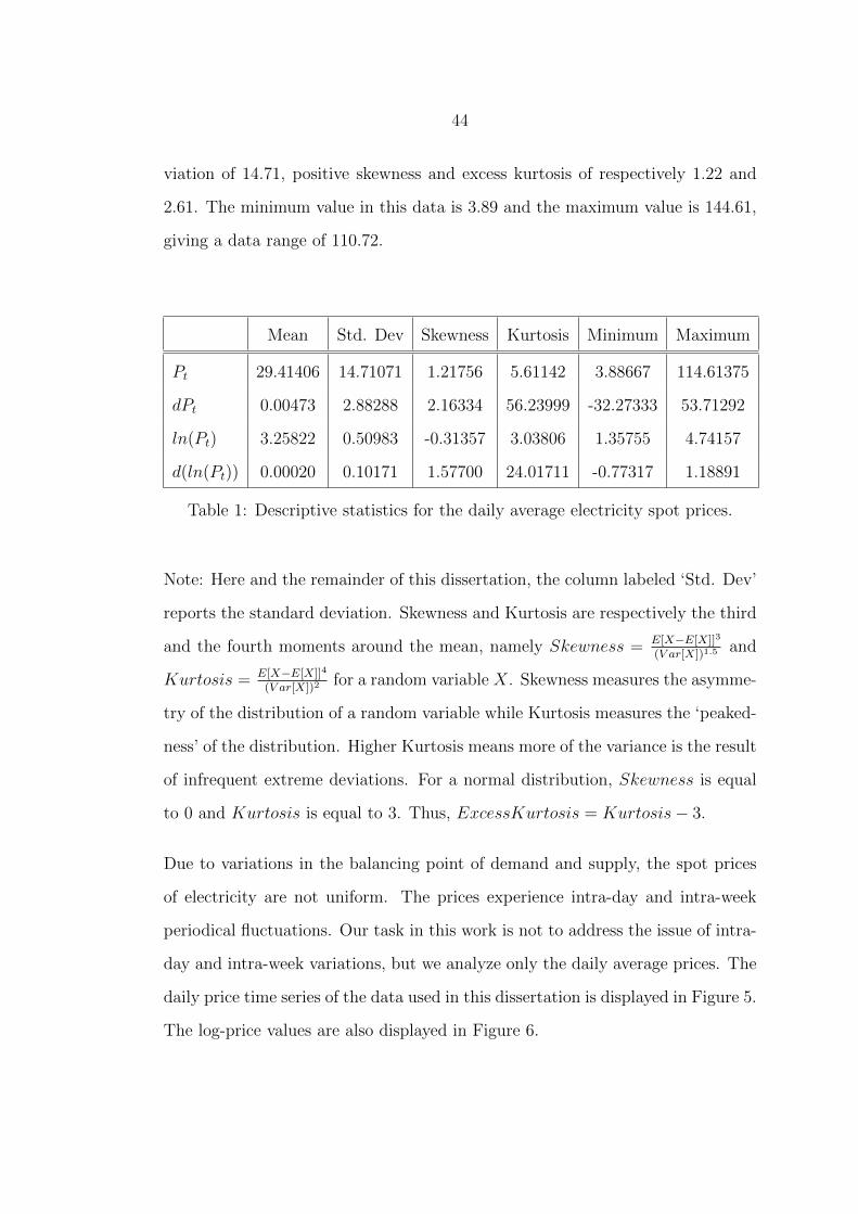
44
viation of 14.71, positive skewness and excess kurtosis of respectively 1.22 and
2.61. The minimum value in this data is 3.89 and the maximum value is 144.61,
giving a data range of 110.72.
Mean Std. Dev Skewness Kurtosis Minimum Maximum
Pt 29.41406 14.71071 1.21756 5.61142 3.88667 114.61375
dPt 0.00473 2.88288 2.16334 56.23999 -32.27333 53.71292
ln(Pt) 3.25822 0.50983 -0.31357 3.03806 1.35755 4.74157
d(ln(Pt)) 0.00020 0.10171 1.57700 24.01711 -0.77317 1.18891
Table 1: Descriptive statistics for the daily average electricity spot prices.
Note: Here and the remainder of this dissertation, the column labeled ‘Std. Dev’
reports the standard deviation. Skewness and Kurtosis are respectively the third
and the fourth moments around the mean, namely Skewness = E[X−E[X]]3
(V ar[X])1.5and
Kurtosis = E[X−E[X]]4
(V ar[X])2for a random variable X. Skewness measures the asymme-
try of the distribution of a random variable while Kurtosis measures the ‘peaked-
ness’ of the distribution. Higher Kurtosis means more of the variance is the result
of infrequent extreme deviations. For a normal distribution, Skewness is equal
to 0 and Kurtosis is equal to 3. Thus, ExcessKurtosis = Kurtosis− 3.
Due to variations in the balancing point of demand and supply, the spot prices
of electricity are not uniform. The prices experience intra-day and intra-week
periodical fluctuations. Our task in this work is not to address the issue of intra-
day and intra-week variations, but we analyze only the daily average prices. The
daily price time series of the data used in this dissertation is displayed in Figure 5.
The log-price values are also displayed in Figure 6.

45
0 500 1000 1500 2000 2500 3000 3500 40000
20
40
60
80
100
120
Time in days[1st Jan, 1999 to 28th Feb, 2009]
Daily
Ave
rage
pric
e[Eu
ro/M
Wh]
Figure 5: Daily average electricity spot price since 1st January, 1999 until 28th
April, 2009 (3712 observations).
0 500 1000 1500 2000 2500 3000 3500 40001
1.5
2
2.5
3
3.5
4
4.5
5
Time in days[1st Jan, 1999 to 28th Feb, 2009]
Log(
Price
s)
Figure 6: The logarithm of electricity prices from which the main features of
electricity market are observed.
All the stylized features of electricity prices as explained in section 1.4.2 are
realized just from first visual inspection of Figures 5 and 6. Seasonality is
46
clear from the two figures where the general path of the prices shows a wave-like
pattern. High volatility and occasional jumps dominate the whole time frame.
Mean-reversion is also quite clear as the price oscillates around the mean level
and whenever there is a spike the price is pulled back to the mean level rapidly
after the spike. We additionally observe that the prices follow an increasing linear
trend mainly being a result of inflation which is a property found in all commodity
markets.
4.2.2 Normality test
In this subsection we analyse whether the returns of electricity spot price are
normally distributed and the prices are log-normally distributed. In the Black-
Schole model the stock prices are assumed to be log-normally distributed. In
order to get the values of the log-price we simply find the logarithm of the spot
price values. To find the returns (log-return) we use its mathematical definition.
That is
rt = lnPtPt−1
where
* rt is the return at the time t,
* Pt is the price value at time t,
* Pt−1 is the price at time t− 1
There is more departure from Normality for the electricity prices. Figure 7 shows
a Normality test carried out for returns of the electricity spot prices from the data.
A solid line connects the 25th and 75th percentile in the data and a dashed line
extends it to the ends of the data. If the returns were indeed normally distributed
the graph would be a straight line as all the points would fall along the dashed

47
line. The fat tails we observe reveal out that this is not the case for electricity
prices. With a probability of 0.006, for example, we find return values which are
higher than 0.2, but the dashed line suggests the probability of such returns to
be zero for perfectly normally distributed data. This behaviour of electricity spot
price returns is in contrast to most financial theories and models which usually
assume the price returns to be normally distributed. That the distribution of
electricity spot price returns deviate from normal is also noticed in Figure 8
where the histogram showing distribution of price returns is superimposed with
a theoretical normal curve.
−0.8 −0.6 −0.4 −0.2 0 0.2 0.4 0.6 0.8 1 1.2
0.0010.0030.01 0.02 0.05 0.10
0.25
0.50
0.75
0.90 0.95 0.98 0.99
0.9970.999
Electricity Price returns
Pro
ba
bili
ty
Normal Probability Plot
Figure 7: Normal probability test for electricity prices returns.

48
−0.8 −0.6 −0.4 −0.2 0 0.2 0.4 0.6 0.8 1 1.20
200
400
600
800
1000
1200
1400
1600
1800
2000
Log−Returns
Freq
uenc
ies
Figure 8: Histogram showing distribution of price returns superimposed with a
theoretical normal curve.
Figure 9 is the histogram of the log-prices also compared to a pure normal dis-
tribution curve. We clearly observe that the log-prices are slightly skewed to the
left which imply the existence of spikes in Nord Pool spot price time series. The
histogram seems to be closer to normal distribution simply because the prices ex-
perience both positive and negative spikes as how it appears in Figure 5. Spiking
is a fundamental property of electricity spot prices. Since our data is on daily
basis, spikes do not last more than one time point (a day in this case). According
to Weron (2006) and as shown in Figure 10, a positive jump is followed by a
negative one of approximately the same magnitude.

49
1 1.5 2 2.5 3 3.5 4 4.5 50
50
100
150
200
250
300
350
400
450
500
Log−prices
Freq
uenc
ies
Figure 9: Histogram for logarithm of spot prices showing distribution of log-prices
for the data, superimposed with the theoretical normal curve.
0 500 1000 1500 2000 2500 3000 3500 4000−0.8
−0.6
−0.4
−0.2
0
0.2
0.4
0.6
0.8
1
1.2
Time in days
Retu
rns
Figure 10: Log-returns price series showing the existence of some price spikes.
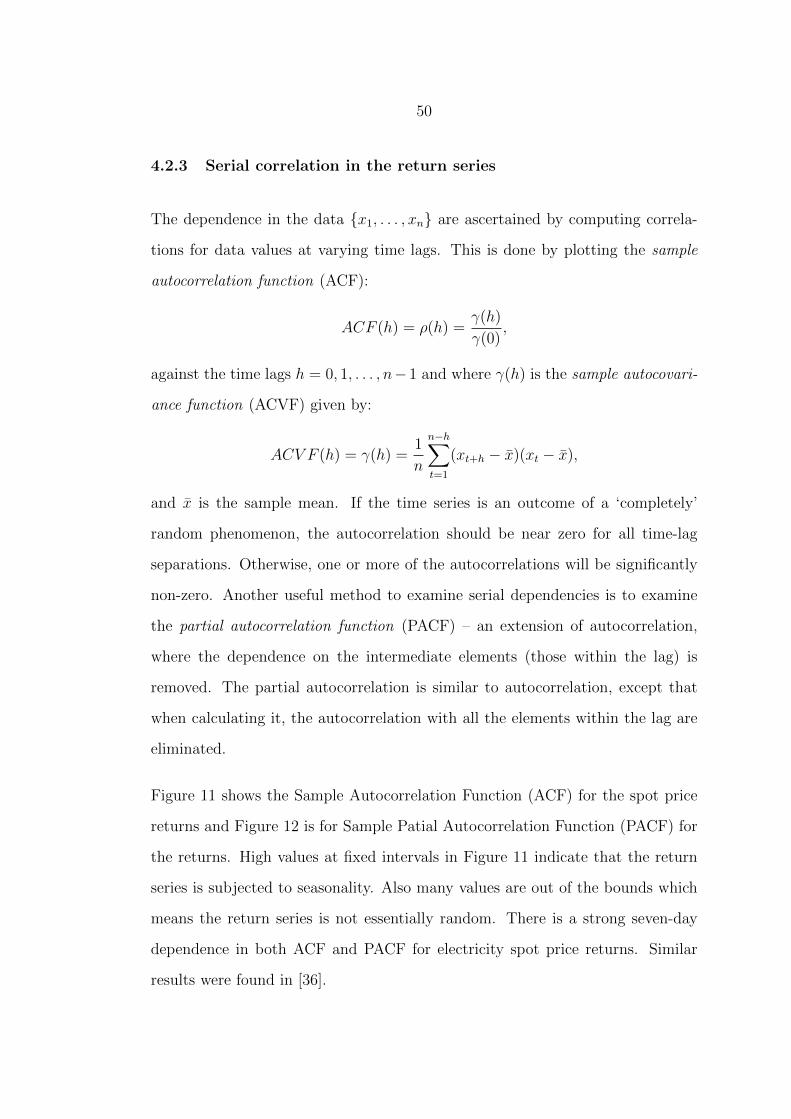
50
4.2.3 Serial correlation in the return series
The dependence in the data x1, . . . , xn are ascertained by computing correla-
tions for data values at varying time lags. This is done by plotting the sample
autocorrelation function (ACF):
ACF (h) = ρ(h) =γ(h)
γ(0),
against the time lags h = 0, 1, . . . , n−1 and where γ(h) is the sample autocovari-
ance function (ACVF) given by:
ACV F (h) = γ(h) =1
n
n−h∑t=1
(xt+h − x)(xt − x),
and x is the sample mean. If the time series is an outcome of a ‘completely’
random phenomenon, the autocorrelation should be near zero for all time-lag
separations. Otherwise, one or more of the autocorrelations will be significantly
non-zero. Another useful method to examine serial dependencies is to examine
the partial autocorrelation function (PACF) – an extension of autocorrelation,
where the dependence on the intermediate elements (those within the lag) is
removed. The partial autocorrelation is similar to autocorrelation, except that
when calculating it, the autocorrelation with all the elements within the lag are
eliminated.
Figure 11 shows the Sample Autocorrelation Function (ACF) for the spot price
returns and Figure 12 is for Sample Patial Autocorrelation Function (PACF) for
the returns. High values at fixed intervals in Figure 11 indicate that the return
series is subjected to seasonality. Also many values are out of the bounds which
means the return series is not essentially random. There is a strong seven-day
dependence in both ACF and PACF for electricity spot price returns. Similar
results were found in [36].

51
0 5 10 15 20 25 30 35 40 45 50−0.2
0
0.2
0.4
0.6
0.8
Lag
Sam
ple
Auto
corre
latio
nSample Autocorrelation Function (ACF)
Figure 11: ACF for price return series showing some important lags. Where most
of the values fall out of the bounds. Seasonality can be observed from the lags
with strong 7 - day dependence.
0 5 10 15 20 25 30 35 40 45 50−0.4
−0.2
0
0.2
0.4
0.6
0.8
1
Lag
Sam
ple
Parti
al A
utoc
orre
latio
ns
Sample Partial Autocorrelation Function
Figure 12: PACF for price return series, where some values are out of the bounds.

52
4.3 Calibration of the model.
We present estimates for the parameters used to generate the coloured noise
process in (11) and (12) and those for the mean-reverting Stochastic Differential
Equation driven by this coloured noise process in (13). For the parameters in the
coloured noise process we rely on the assumption that the length of the correlation
time τ is equal to 7 as explained in section 3.4 where other parameters α1 and
α2 were then estimated from this value of τ .
For the Stochastic Differential Equation we first removed the trend as shown in
Figure 13 and then we cleared out the spikes as shown in Figure 14. The spikes
were removed out since they were considered as outliers in the data set and
retaining them could distort the parameter estimation procedure. The process
of removing the spike considered one and a half (1.5) standard deviation of the
moving window of seven days as the threshold value for determining the existence
of spikes in the window. The positions handling values that are higher or lower
from mean with a difference greater than this threshold value were considered as
spikes. The position with spike was then substituted with a mean value of the
window. With this approach both positive and negative spikes were considered.
Then the estimates for the mean-reversion level (X) and volatility (σ) were taken
as the averages of respectively the mean values and standard deviation of an
analysis window of 90 days which is approximate to 3 months period. The mean
reversion rate (κ) was continuously estimated depending on previous 90 days
data by the Maximum Likelihood method described in section 3.4.1 and its mean
value is 0.4716 which can be used in further computations. The results for the
estimated parameters are in summary presented in Table 2.
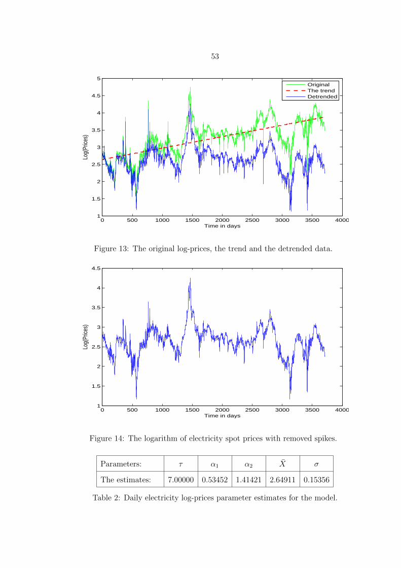
53
0 500 1000 1500 2000 2500 3000 3500 40001
1.5
2
2.5
3
3.5
4
4.5
5
Time in days
Log(
Price
s)
OriginalThe trendDetrended
Figure 13: The original log-prices, the trend and the detrended data.
0 500 1000 1500 2000 2500 3000 3500 40001
1.5
2
2.5
3
3.5
4
4.5
Time in days
Log(
Price
s)
Figure 14: The logarithm of electricity spot prices with removed spikes.
Parameters: τ α1 α2 X σ
The estimates: 7.00000 0.53452 1.41421 2.64911 0.15356
Table 2: Daily electricity log-prices parameter estimates for the model.

54
4.4 Analysis of Coloured Noise used in Simulation
As described in section 3.3 the coloured noise used in this work is a stationary,
zero-mean and correlated Gaussian markov process which by [5] it is essentially
in the form of Ornstein-Uhlenbeck process as the one in equation (5) and/or (7).
This fluctuation process is called “coloured noise” in analogy with the effects of
filtering on white light [18]. We adopt the term ‘filtering’ in our study and apply
it twice on white noise to get more correlated noise process as in [10]. In order
to generate the coloured noise in two-step filtering for ζ1(t) and ζ2(t) from the
white noise ξ(t) the following algorithm found in [5, 13] was used:
At the sample points tn(t0 < t1 < . . . < tN−1),
ζ1(0) = sξ(0)
ζ1(n) = ρnζ1(n− 1) +√
1− ρ2nsξ(n)
where ξ are independent Gaussian random numbers with zero mean and unit
variance, s is the standard deviation for the coloured noise and ρn are the corre-
lation coefficients given by ρn = e−|tn−tn−1|/τ . The algorithm is similarly used to
generate ζ2(n) with ξ(n) being replaced by ζ1(n).
Figure 15 shows the plots for white noise ξ(t) and coloured noise ζ1(t), ζ2(t)
separately and combined ξ(t) and ζ2(t) in Figure 16. An increase in the autocor-
relation due to filtering of white noise is seen in Figure 17 and Figure 18.
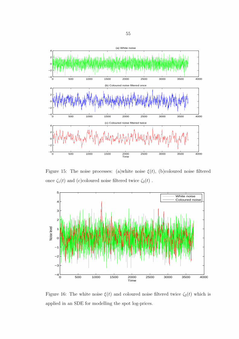
55
0 500 1000 1500 2000 2500 3000 3500 4000−4
−2
0
2
4(a) White noise
0 500 1000 1500 2000 2500 3000 3500 4000−4
−2
0
2
4(b) Coloured noise filtered once
0 500 1000 1500 2000 2500 3000 3500 4000−4
−2
0
2
4(c) Coloured noise filtered twice
Time
Figure 15: The noise processes: (a)white noise ξ(t), (b)coloured noise filtered
once ζ1(t) and (c)coloured noise filtered twice ζ2(t) .
0 500 1000 1500 2000 2500 3000 3500 4000−4
−3
−2
−1
0
1
2
3
4
5
Time
Noise
leve
l
White noiseColoured noise
Figure 16: The white noise ξ(t) and coloured noise filtered twice ζ2(t) which is
applied in an SDE for modelling the spot log-prices.
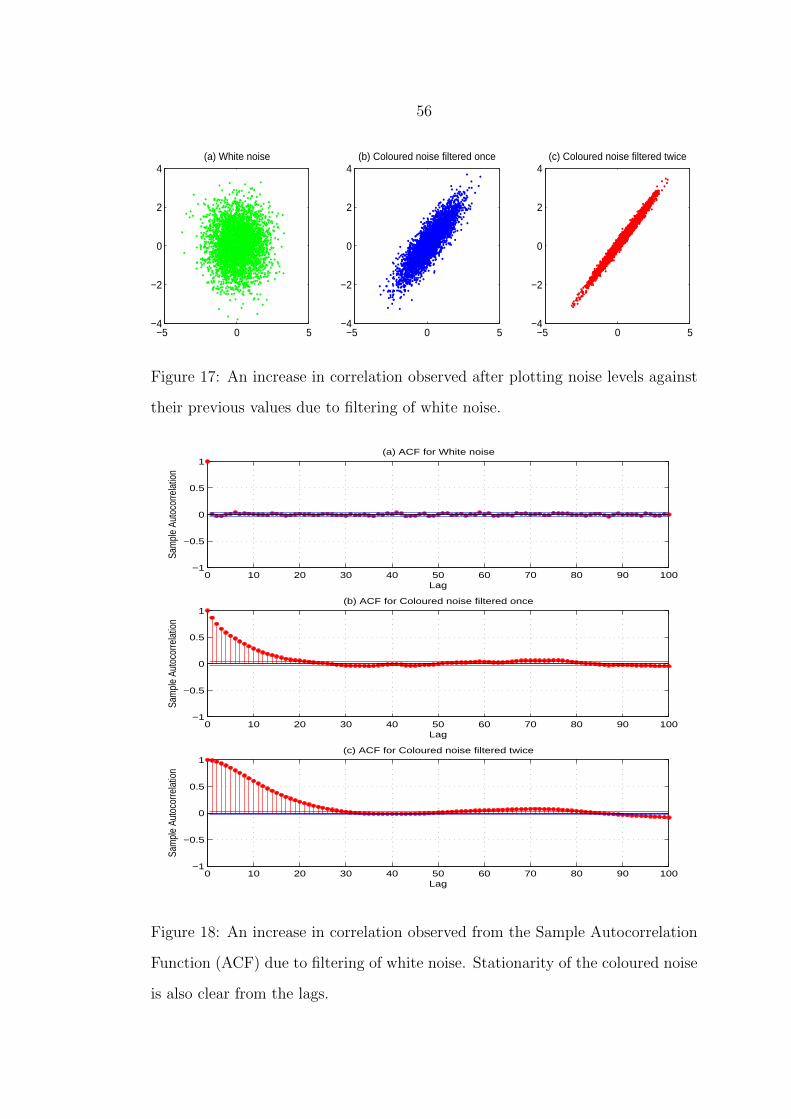
56
−5 0 5−4
−2
0
2
4(a) White noise
−5 0 5−4
−2
0
2
4(b) Coloured noise filtered once
−5 0 5−4
−2
0
2
4(c) Coloured noise filtered twice
Figure 17: An increase in correlation observed after plotting noise levels against
their previous values due to filtering of white noise.
0 10 20 30 40 50 60 70 80 90 100−1
−0.5
0
0.5
1
Lag
Sam
ple
Auto
corre
latio
n
(a) ACF for White noise
0 10 20 30 40 50 60 70 80 90 100−1
−0.5
0
0.5
1
Lag
Sam
ple
Auto
corre
latio
n
(b) ACF for Coloured noise filtered once
0 10 20 30 40 50 60 70 80 90 100−1
−0.5
0
0.5
1
Lag
Sam
ple
Auto
corre
latio
n
(c) ACF for Coloured noise filtered twice
Figure 18: An increase in correlation observed from the Sample Autocorrelation
Function (ACF) due to filtering of white noise. Stationarity of the coloured noise
is also clear from the lags.

57
4.5 Model simulation, results and comparison
The parameters obtained in Table 2 were used for simulating the electricity spot
price time series using Matlab software. The white noise was taken in its discrete
form, that is, random numbers generated by the function randn found in Matlab.
Simulation of the coloured noise process followed the algorithm described in the
previous section. The log-prices were then simulated following the mean-reverting
Stochastic Differential Equation (13) in which the coloured noise process was
attached and the trend was then restored back. The required prices were then
simulated out of these log-prices by taking out the logarithm.
Figure 19 shows the real (original) log-prices (in blue colour) and the simulated
log-prices with the trend restored (in green colour) on the same plane. The spot
prices from real data (in blue colour) and the simulated prices (in red colour) were
together plotted as in Figure 20. Figure 21 shows the histograms of both real and
simulated spot prices in a comparable manner. The histograms of the real and
simulated spot prices appear to be of the same nature in distribution. For more
comparison between the real and simulated spot prices we have presented the
histogram of the residuals which are the differences of real and simulated prices
as in Figure 22. We see that much of the residuals are concentrated at zero with
a standard deviation of 14.32. Table 3 gives the statistical comparison between
real and simulated spot prices focusing on the mean, standard deviation, kurtosis
and skewness.

58
0 500 1000 1500 2000 2500 3000 3500 40001
1.5
2
2.5
3
3.5
4
4.5
5
Time in days
Log(
Price
s)
RealSimulated
Figure 19: Simulation results for logarithm of Prices vs real (original) log-prices.
0 500 1000 1500 2000 2500 3000 3500 40000
20
40
60
80
100
120
Time in days
Daily
Ave
rage
pric
e[Eu
ro/M
Wh]
Real priceSimulated price
Figure 20: Simulated Electricity Spot Prices Time-series versus Real Prices.
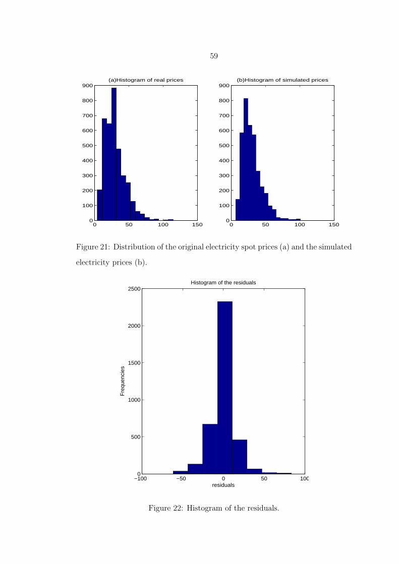
59
0 50 100 1500
100
200
300
400
500
600
700
800
900(a)Histogram of real prices
0 50 100 1500
100
200
300
400
500
600
700
800
900(b)Histogram of simulated prices
Figure 21: Distribution of the original electricity spot prices (a) and the simulated
electricity prices (b).
−100 −50 0 50 1000
500
1000
1500
2000
2500
residuals
Fre
quen
cies
Histogram of the residuals
Figure 22: Histogram of the residuals.

60
Real prices Simulated prices
Mean 29.41406 29.76591
Std. Dev 14.71071 13.85724
Skewness 1.21756 1.27255
Kurtosis 5.61142 5.37944
Minimum 3.88667 6.35211
Maximum 114.61375 100.87738
Table 3: Real (original) spot prices data vs Simulated data.
4.6 Application on Pure trading
By pure-trading we mean the price series (behaviour) independent of the influence
of the trend and seasonality. In one of the recent studies, [?] was able to get such
a series by doing detrending and two steps of deseasonalizing. First he removed
the weekly and monthly seasonality by an additive model and next by building
regression model with the use of background variables (temperatures and water
reservoirs). Thou he analysed the prices differently in each country we adopt
the system prices with background variables taken from Norway. The series he
obtained is as given in Figure 23. We used the approaches of section 4.5 on this
series and obtained the results as ploted in Fugure 24 and corresponding statistics
in Table 4. Since the series has negative values which are not suitable for our
model, converting them into some positive values by some additions before and
then subtraction after simulation was necessary. Though there appears frequent
short spikes for simulated data, the simulation was able to produce spikes which
are as high as the original spikes. Table 4 shows close results for the simulated
and original series in the statistics as well.

61
0 500 1000 1500 2000 2500 3000 3500 4000−40
−30
−20
−10
0
10
20
30
40
50
Time in days
Pure
−pric
e se
ries[
Euro
/MW
h]
Figure 23: Pure price series since 1st January, 1999 until 28th April, 2009.
0 500 1000 1500 2000 2500 3000 3500 4000−40
−30
−20
−10
0
10
20
30
40
50
Time in days
Pure
−pric
e se
ries[
Euro
/MW
h]
Real priceSimulated price
Figure 24: Simulated vs real (original) pure price series.

62
Real pure-prices Simulated pure-prices
Mean 0.72864 0.83423
Std. Dev 7.47424 8.94825
Skewness 0.92309 0.95938
Kurtosis 6.97564 5.51393
Minimum -30.46631 -19.69480
Maximum 46.23567 49.76592
Table 4: Real (original) pure-prices data vs Simulated data.
4.7 Forward price
The only optimal hedging strategy in electricity markets is the use of forwards.
Other usual hedging strategies adopted in other financial assets, such as holding
certain quantities of the underlying, which is electricity in this case, is not a fea-
sible solution. The reason behind is, as earlier mentioned, that electricity can not
be physically and economically stored. It must be consumed almost immediately,
once purchased. In this subsection we derive a formula for estimating the forward
prices based on our model.
The price at time t of the forward expiring at time T is obtained as the expected
value of the spot price at expiry under an equivalent Q-martingale measure,
conditional on the information set available up to time t; namely
F (t, T ) = EQt [ST |Ft] (22)
Thus, we need to replace Xt = lnSt and integrate the resulting SDE in order to
extract ST and later calculate its expectation.
Regarding the expectation, we must calculate it under an equivalentQ-martingale
measure. In a complete market this measure is unique, ensuring only one arbitrage-
free price of the forward. However, in incomplete markets (such as the electricity

63
markets) this measure is not unique, thus we are left with the difficult task of
choosing an appropriate measure for the particular market in question. Another
approach, common in the literature, is simply to assume that we are already
under an equivalent measure, and thus proceed to perform the pricing directly.
This latter approach would rely however in calibrating the model through im-
plied parameters from a liquid market. This is certainly difficult to do in young
markets and those which are about to be initiated, as there will be no liquidity
of instruments that would enable us to do this. But for the case of Nord Pool
where our reference data have been taken, this is possible as there is sufficient
liquidity of the market.
We follow instead Lucia and Schwartz approach in [24], which consists of incor-
porating a market price of risk in the drift, such that
ˆX ≡ X − λ∗ and λ∗ ≡ λσκ
where λ denotes the market price of risk per unit risk linked to the state variable
Xt. This market price of risk, to be calibrated from market information, pins
down the choice of one particular martingale measure. Under this measure now
we may then rewrite the stochastic process in (13) for Xt as
dXt = κ( ˆX −Xt)dt+ σζ2(t)dt (23)
where the long term mean is assumed to have some seasonality factor g(t), that
is
ˆX =1
κ
dg
dt+ g(t)− λσ
κ
and ζ2(t) is the coloured noise process in which the incorporated dW (t) is the
increment of Brownian motion in the Q-measure specified by choice of λ. Inte-
grating the process (23) from t to T we get
XT = Xte−κ(T−t) +
∫ T
t
κe−κ(T−s) ˆXds+ σ
∫ T
t
e−κ(T−s)ζ2(s)ds (24)

64
We now introduce the market price of risk and we get
XT = g(T )+(Xt−g(t))e−κ(T−t)−λ∫ T
t
σe−κ(T−s)ds+σ
∫ T
t
e−κ(T−s)ζ2(s)ds (25)
Further manipulation with the expansion of ζ2(s) gives
XT = g(T ) + (Xt − g(t))e−κ(T−t) − λ∫ T
t
σe−κ(T−s)ds+ (1
τ− κ)−2 1
τσα1α2
×∫ T
t
(1− k
τ+ κk)e
kτ−κk − (1 +
T − tτ− 2k
τ− κ(T − t) + 2κk)e−
(T−t)τ−κk+ 2k
τ dWk(26)
Since ST = eXT , we can replace (26) and then substitute into (22) to get the
forward price
F (t, T ) = EQt [ST |Ft]
= e−λ∫ Tt σe−κ(T−s)dsG(T )
(S(t)
G(t)
)e−κ(T−t)
Et[eaσ
∫ Tt (1− k
τ+κk)e
kτ −κk−(1+T−t
τ− 2kτ−κ(T−t)+2κk)e−
(T−t)τ −κk+2k
τ dWk |Ft]
(27)
where a = ( 1τ− κ)−2 1
τα1α2
In order to evaluate the expectation above we make use of Ito’s Isometry theory
and probability theory, which is stated in Theorem 2 below.
Theorem 2 If f belongs to H2[0, T ], the space of random functions defined for
all t in [0, T ], and
∫ T0E[f(t)]2dt <∞, then
E[∫ T
0f(t)dWt] = 0 and E[(
∫ T0f(t)dWt)
2] =∫ T
0E[f(t)]2dt
Thus the expectation is obtained as
Et[eaσ
∫ Tt (1− k
τ+κk)e
kτ −κk−(1+T−t
τ− 2kτ−κ(T−t)+2κk)e−
(T−t)τ −κk+2k
τ dWk |Ft]
= ea2σ2
2
∫ Tt (1− k
τ+κk)e
kτ −κk−(1+T−t
τ− 2kτ−κ(T−t)+2κk)e−
(T−t)τ −κk+2k
τ dk
≈ e( 1τ−κ)−4 1
τ2σ2
2α21α
22 (28)
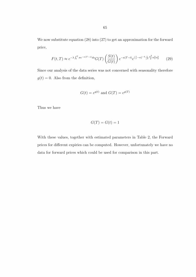
65
We now substitute equation (28) into (27) to get an approximation for the forward
price,
F (t, T ) ≈ e−λ∫ Tt σe−κ(T−s)dsG(T )
(S(t)
G(t)
)e−κ(T−t)e( 1
τ−κ)−4 1
τ2σ2
2α21α
22 (29)
Since our analysis of the data series was not concerned with seasonality therefore
g(t) = 0. Also from the definition,
G(t) = eg(t) and G(T ) = eg(T )
Thus we have
G(T ) = G(t) = 1
With these values, together with estimated parameters in Table 2, the Forward
prices for different expiries can be computed. However, unfortunately we have no
data for forward prices which could be used for comparison in this part.

CHAPTER FIVE
CONCLUSION AND RECOMMENDATIONS
4.1 Conclusion.
In this dissertation, we have developed a stochastic mean-reverting model driven
by coloured noise process in modelling of electricity spot price time series data.
The data used were collected from Nord Pool market, the Elspot. Analysis of
these data was carried out and some important statistical behaviours such as
mean-reversion, spikes, seasonality and the trend were found as in Figures 5
and 6. Also we performed the normality test and ploted the autocorrelation
functions as shown in Figures 7, 11 and 12. And thus the data was found to
be appropriate for stochastic modelling. The coloured noise process were also
mathematically described as in section 3.3 and analysed in section 4.4. The
analysis showed significant autocorrelation within the coloured noise process as
compared to white noise where there is no any significant autocorrelation as
shown in Figures 17 and 18. The model was then used to simulate the spot
prices. Matlab software were used to do both data simulation and ploting of the
corresponding figures.
Results from the model show that the simulated price series is similar to the
real evolution of electricity spot price time series observed in the market, since it
covers the price series interval both above and below and was able to reflect some
higher values (spikes) of the price series as it appears in Figures 19 and 20. As
to what is diplayed in Table 3, the decriptive statistics for both emperical and
those from the simulated data are also close to each other, indicating that the
model has been a good representation of the real spot price process. Concerning
the forward price, the prices depend much on the market price of risk which is
inevitable for incomplete markets. These forward prices are very useful since

67
power markets are one hour/day ahead markets for spot markets.
Though the data used in this work were from Scandinavian countries, the rel-
evance of this study to developing countries like those found in Sub-Saharan
Africa and Tanzania in particular was insisted as found in the first chapter of
this dissertation.
4.2 Recommendations and Future work.
The application of coloured noise process in market price models such as those
of electricity seems to be a novel idea. From the results of this work it has
been shown that the coloured noise process is appropriate in modelling electricity
prices. We hereby recommend that;
1. Power generating companies, electricity traders and all the participants in
electricity markets should consider the results of this work for price fore-
casting and proper pricing of electricity.
2. Tanzania and other developing countries in general should speed up the grid
interconnection among different regions and liberalize the power sector for
efficient and reliable power supply to consumers.
Apart from all the efforts which have been taken by various scholars to model the
spot prices of electricity, including this work, there are always holes left uncovered.
We recommend in future, therefore, first to take more steps in ‘filtering’ of the
coloured noise process in order to reduce the frequency of spikes observed in the
simulation. Secondly to combine the coloured noise approach together with other
modelling methods such as Multifactor models and the Structural models so that
we may come up with a more efficient model.

68
References
[1] Arnold, L. (1974), Stochastic Differential Equations: Theory and Ap-
plications, London, Wiley pp. 1–228.
[2] Bacon, R. (1999), “Global Energy Sector Reform in Developing Countries”,
A Scorecard. Report No. 219-99. Washington, D.C.: UNDP/World Bank,
http://earthtrends.wri.org/pdf library/feature/gov fea power.pdf retrieved on
Friday, 18th December, 2009
[3] Barlow, M. T. (2002), “A Diffusion Model for Electricity Prices”, Journal of
Mathematical Finance, ScienceDirect, Volume 12(2002) pp. 287-298
[4] Barlow, M. T., Gusev, Y. and Manpo, L. (2002), “Calibration of multifac-
tor models in electricity markets”, International Journal of Theoretical and
Applied Finance, 7(2004), pp. 101–120.
[5] Bartosch, L. (2001), “Generation of Colored Noise”, International Journal
of Modern Physics C, World Scientific Publishing Company, Volume 12, No.
6 (2001) 851-855
[6] Barz, G. (1999), “Stochastic Financial Models for Electricity Derivatives”,
University of Stanford, Ph.D. Thesis.
[7] Barz, G. and Johnson, B. (1999), “Selecting Stochastic Process for Modelling
Electricity Prices”, Energy Modelling and the Management of Uncertainty,
Risk Publications
[8] Bishwal, J. P. N. (2008), Parameter Estimation in Stochastic Differ-
ential Equations, Berlin and Heidelberg, Springer-Verlag

69
[9] Carnero, M. A., Koopman, S. J. and Ooms, M. (2003), “Periodic het-
eroskedastic RegARFIMA models for daily electricity spot prices”, Tinbergen
Institute Discussion Paper, TI 2003–071/4.
[10] Charles, W. M. (2008), “Coloured noise for dispersion of contaminants in
shallow waters”, Journal of Applied Mathematical Modelling, ScienceDirect,
Volume 33(2009) 1158-1172
[11] Cuaresma, J. C., Hlouskova, J., Kossmeier, S. and Obersteiner, K. (2004),
“Forecasting electricity spot prices using linear univariate time-series mod-
els”, Applied Energy 77, 87–106.
[12] Eydeland, A. and Geman, H. (1999), Fundamentals of Electricity
Derivatives., Energy modeling and management of uncertainty. RISK
books.
[13] Finch, S. (2004), “Ornstein-Uhlenbeck Process”, Department of Statistics
Harvard University,
http://algo.inria.fr/csolve/ou.pdf retrieved on Monday, 14th December, 2009
[14] Gardiner, C. W. (1997), Handbook of Stochastic Methods for Physics,
Chemistry and the Natural Sciences, Berlin, Heidelberg and New York,
Springer-Verlag
[15] Geman H. (2002), “Towards a European Market of Electricity :Spot and
Derivatives Trading”, University Paris IX Dauphine and ESSEC,
http://www.iea.org/textbase/work/2003/powergen/geman.pdf retrieved on
Monday, 14th December, 2009
[16] Geman, H. and Roncoroni, A. (2006), “Understanding the fine structure of
electricity prices”, Journal of Business, 79(3) 1225-1262.
[17] Haeussler, F. (2008), “Modeling electricity spot prices and Risk-neutral pric-
ing of options”, University of Wisconsin-Milwaukee, Master thesis

70
[18] Hanggi, P. and Jung, P. (1995), Colored Noise in Dynamical Systems,
Augsburg Germany, John Wiley & Sons Inc.
[19] Janczura, J. and Weron, R. (2009), “Regime-switching models for electricity
spot prices: Introducing heteroskedastic base regime dynamics and shifted
spike distributions”, Munich Personal RePEc Archive, MPRA Paper No.
18784
http://mpra.ub.uni-muenchen.de/18784/ retrieved on Monday, 15th Febru-
ary, 2010
[20] Kaminski, V. (1999), Managing Energy Price Risk, London, Risk Books
[21] Kanamura, T. and Ohashi, K. (2004), “A Structural Model for Electric-
ity Prices with Spikes: Measurement of jump risk and optimal policies for
hydropower plant operation”, Working paper, Hitotsubashi University
[22] Karakastani, N. and Bunn, D. W. (2004), “Modelling the volatility of spot
electricity prices”, EMG Working Paper, London Business School
[23] Knittel, C. R. and Roberts, M. R. (2001), “An empirical examination of
deregulated electricity prices”, Working Paper, University of California En-
ergy Institute
[24] Lucia, J. J. and Schwartz, E. S. (2002), “Electricity prices and power deriva-
tives: Evidence from the nordic power exchange.”, Review of Derivatives
Research, Volume 5, No.1
[25] Mavrou, V. (2006), “Modelling the Dynamics of Electricity Prices”, Univer-
sity of Zurich, Master thesis 2006
[26] Meyer-Brandis, T. and Tankov, P. (2007), “Multi-factor jump-diffusion mod-
els of electricity prices”, Working paper, Universite Paris VII, France.

71
[27] Nordic Electricity Regulators (NordREG),The Nordic Electricity Market
https://www.nordicenergyregulators.org
/The-Development-on-the-Nordic-Electricity-Market retrieved on Tuesday,
15th December, 2009
[28] Oksendal, B. K. (2000), Stochastic Differential Equations: An Intro-
duction with Applications, Heidelberg and New York, Springer-Verlag
[29] Oparaku, O. U. (2006), “Solar-photovoltaics in the deregulated electricity
industry of developing countries”, Proceedings of the International Confer-
ence on Renewable Energy for Developing Countries-2006, National Centre
for Energy Research and Development, University of Nigeria, Nsukka
[30] Shreve, S. E. (2008), Stochastic Calculus for Finance II: Continuous-
Time Models, Springer-Verlag Publishers
[31] Tanzania Electric Supply Company (TANESCO): Generation,Transmission,
Distribution and Services,
http://www.tanesco.co.tz/ retrieved on Monday, 14th December, 2009
[32] Taylor, H. M. and Karlin, S. (1998), An Introduction to Stochastic
Modeling, San Diego and California USA, Academic Press
[33] Vehvilainen I. and Pyykkonen T. (2005), “Stochastic factor model for elec-
tricity spot price-the case of the Nordic market”, Journal of energy eco-
nomics, Volume 27.
[34] Wangensteen, I. (2006), Power markets, Trondheim Norway, NTNU-
Institutt for elkraftteknikk
[35] Weron, R.(2005), “Heavy tails and electricity prices”, The Deutsche Bun-
desbank’s 2005 Annual Fall Conference (Eltville, 10-12 November 2005)

72
[36] Weron, R. (2006), Modeling and Forecasting electricity loads and
prices: A Statistical Approach, West Sussex England, John Wiley and Sons
Ltd.
[37] Weron, R. (2008), “Heavy-tails and regime-switching in electricity prices”,
Munich Personal RePEc Archive, MPRA Paper No. 10424
http://mpra.ub.uni-muenchen.de/10424/ retrieved on Monday, 15th Febru-
ary, 2010
[38] WIKIPEDIA-The Free Encyclopedia: Electricity market,
http://en.wikipedia.org/wiki/Electricity market retrieved on Monday, 14th
December, 2009