Commercial Sector Modelling of PV and Electricity Prices ...apvi.org.au/.../Commercial-Sector-Modelling-of-PV-and-Electricity... · Modelling of PV and Electricity ... generated by

AUTHORS:Graham Mills (APVA); Robert Passey, Muriel Watt & Simon Franklin (IT Power Australia);Anna Bruce (UNSW); Warwick Johnson (SunWiz)

With support from

Modelling of PV andElectricity Prices inthe AustralianCommercial SectorBy

The Australian PV Association

November 2011

ACKNOWLEDGEMENTS

The model used to prepare the analyses for this report was developed with fundingassistance predominantly from the Australian Solar Institute but also from the Australian PVAssociation, and with data sourced from APVA members and literature sources.

The model was initially developed in early 2010 and updated in mid 2011. However, sincePV costs and performance continue to improve, values in the graphs should be read from therelevant current date.

About the Australian PV Association

The APVA is an Association of companies, government agencies, individuals, university andother research groups with an interest in photovoltaic solar electricity research, technology,manufacturing, systems, policies, programs and projects. In addition to Australian activities, weprovide the structure through which Australia participates in the International Energy Agency(IEA) Photovoltaic Power Systems programme (PVPS).

Our work is intended to be apolitical and of use, not only to our members, but also to thegeneral community. We are not a traditional lobby group, but instead focus on data analysis,independent and balanced information and collaborative research, both nationally andinternationally.

Our reports, media releases and submissions can be found at: www.apva.org.au

COPYRIGHT This report is copyright of the Australian PV Association. Theinformation contained therein may freely be used but all such use should cite thesource as “APVA, 2011, Modelling of PV & Electricity Prices in the AustralianCommercial Sector, 2011”.

Contents

ACKNOWLEDGEMENTS ......................................................................................................................................... 2

About the Australian PV Association .............................................................................................................. 2

PV in the Commercial Sector.............................................................................................................................. 4

Background ........................................................................................................................................................ 5

Description of the model ...................................................................................................................................... 6

Model Inputs ..................................................................................................................................................... 6

Model Outputs.................................................................................................................................................. 8

Results........................................................................................................................................................................... 8

Base Case System.......................................................................................................................................... 9

Sensitivity Analysis ............................................................................................................................................... 12

Module Efficiency........................................................................................................................................ 13

Module Cost .................................................................................................................................................... 14

Finance Costs ................................................................................................................................................. 15

Purchasing power of the AUD ........................................................................................................... 16

Conclusions .............................................................................................................................................................. 18

Uses for the Model ..................................................................................................................................... 19

Next Steps........................................................................................................................................................ 19

Sunpower panels installed onCrowne Plaza in Alice Springs,NT by CAT Projects(Photo: Sunpower Corp)

PV in the Commercial SectorThe APVA has developed a set of techno-economic projection models to inform stakeholders

as to likely changes in the cost of electricity generated by PV, compared to prevailing gridelectricity prices. Three models were developed, one for residential systems, one for systemson commercial buildings, and another for systems designed for generation on a large scale. Theresidential and commercial systems are compared to the prices of grid electricity understandard electricity supply arrangements, whereas the large-scale model compares the cost ofPV-electricity to wholesale electricity market prices.

Note that the residential and commercial comparisons implicitly assume that all electricitygenerated by the system is valued at the relevant retail tariff, whilst in practice PV systemowners may receive little or no payment for electricity which is not used on site. Also, the lifecycle cost of PV electricity is calculated over a 25 year period, while many businesses expect apayback period on their investment of less than 10 years.

Each of these three models has the same functionality, but is structured to reflect thediffering cost arrangements for each application. The models exclude government subsidy (eg.Solar Credits) and special tariff arrangements, so as to model the underlying economic case forcurrent and future investments in PV. Achieving grid parity is a milestone now beginning to bereached for distributed PV systems, but it may not alone result in cost-effective or guaranteeddeployment. Both technical changes to the grid and regulatory changes to the market are likelyto be required before distributed PV systems can be widely deployed.

PV remains a relatively new technology, with much research and development still required.Nevertheless, it is one of the most versatile and promising of the renewable energy technologiesnow available. The results presented herein provide an indication of its prospects in theAustralian commercial sector. The underlying data were sourced from APVA members andpublically available information. The results presented are for the purposes of informingstakeholders and the interested public. They are general in nature and subject to a number ofunderlying assumptions. As such, readers should not take these results as representingfinancial or investment advice.

Background

The commercial sector accounts for 10% of Australia’s greenhouse gas emissions, with 80%of the sector’s emissions resulting from electricity use. Commercial electricity use is 22% of thetotal electricity use in Australia and is expected to grow to 32% over the next 2 decades1.

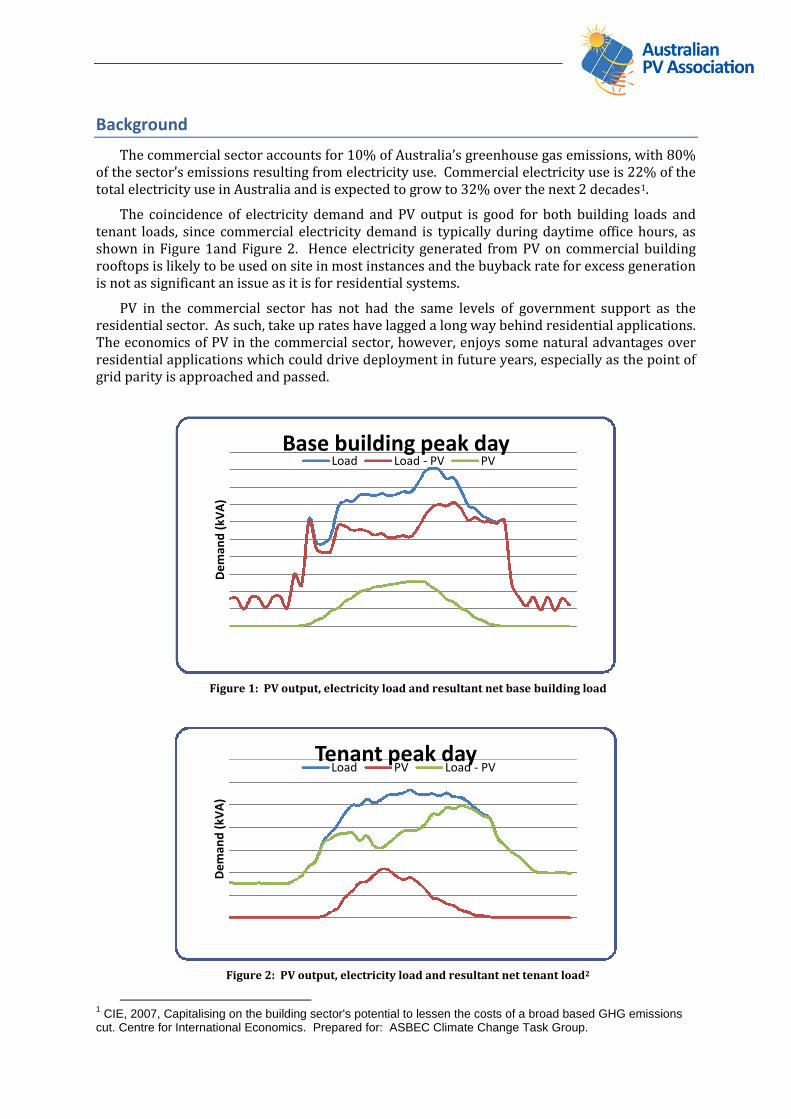
The coincidence of electricity demand and PV output is good for both building loads andtenant loads, since commercial electricity demand is typically during daytime office hours, asshown in Figure 1and Figure 2. Hence electricity generated from PV on commercial buildingrooftops is likely to be used on site in most instances and the buyback rate for excess generationis not as significant an issue as it is for residential systems.

PV in the commercial sector has not had the same levels of government support as theresidential sector. As such, take up rates have lagged a long way behind residential applications.The economics of PV in the commercial sector, however, enjoys some natural advantages overresidential applications which could drive deployment in future years, especially as the point ofgrid parity is approached and passed.

Figure 1: PV output, electricity load and resultant net base building load

Figure 2: PV output, electricity load and resultant net tenant load2

1CIE, 2007, Capitalising on the building sector's potential to lessen the costs of a broad based GHG emissions

cut. Centre for International Economics. Prepared for: ASBEC Climate Change Task Group.

De

man

d(k

VA

)

Base building peak dayLoad Load - PV PV

De

man

d(k

VA

)

Tenant peak dayLoad PV Load - PV

The natural benefits enjoyed by PV applications in the commercial sector include: thebenefits of depreciation and other tax advantages; economies of scale; prospects for buildingintegration, as well as the natural match between PV output and load. This natural matchbetween output and load, combined with the kVA demand tariffs levied on commercial users,creates the opportunity for additional value to accrue to the system owner over and above thevalue of energy generated. These natural advantages create the opportunity for the commercialsector to rise to prominence especially as government subsidies, rebates, and preferential feedin tariffs are reduced in the residential sector. Nevertheless, much of the institutional capacitythat has allowed residential PV prices to fall rapidly in recent years has not yet been establishedin the commercial sector, so that projects are still individually developed. For instance,standardised procedures and costs for grid connection approvals, for installation on differentroof types and for systems supplying tenant vs building loads would reduce up-front projectcosts and thence allow the economies of scale of commercial systems to be captured.

Description of the modelThe results presented herein were obtained from the APVA’s commercial system cost

projection model which is an integrated system cost and discount cash flow model implementedin Excel and controlled by VBA Macros. For detailed information regarding the methodologyused, interested readers should consult “A Manual for the Economic Evaluation of EnergyEfficiency and Renewable Energy Technologies” published by the US National Renewable EnergyLaboratory3

Model Inputs

System Scenarios

The model operates via user definition of a system scenario. The variables selected by theuser for this system then define the default cost, energy, and financial parameters from whichthe model produces its results. The user selects from a drop down table which provides thefollowing choices for this purpose:

Technology type: thin film, polycrystalline, monocrystalline and high efficiency silicon4

Nominal system size: 100kW, 250kW or 500kW Location: Brisbane, Sydney or Melbourne5

Financing: 100% debt (risk free), 100% debt, 100% equity, 50% debt / 50% equity Development model: Standardised commercial systems, individually designed

commercial systems.

Once the system scenario has been specified, the model selects the relevant PV equipmentdata (module efficiency, module area, Voc, Module weight and average annual performancedegradation) and financial data (landed module cost, inverter cost and BOS costs) from a set ofdefault pre-programmed values contained within the model. Note that all models assumenorth-facing PV arrays at latitude angle.6

The model does not include the costs of connecting to the network, because this cost is verysite-specific. For example, for a system greater than 30kW, it can vary between around

2Lam, T., 2008, PV Power System Uptake in the Commercial Building Sector, Final Year Thesis, School of PV &

RE Engineering, UNSW.3

Short W, Packey D, Holt T, A Manual for the Economic Evaluation of Energy Efficiency and Renewable EnergyTechnologies, National Renewable Energy Laboratory, 1995. www.nrel.gov/docs/legosti/old/5173.pdf4

These differ in terms of efficiency, cost, area, open circuit voltage (Voc) and weight.5

These differ in the annual average insolation and the performance ratio.6

Note that this model does not attempt to duplicate what detailed PV performance models such as PVSyst offer.It is envisaged that data from such models can readily be inserted at the front end of this model if required.

$100,000 (for a connection of a lone system directly to the network) and approaching zero(where the system connects on the load side of the meter and its maximum output is less thanthe minimum load – and so the system would never export to the network)

Key Cost / Financial Parameters

In addition to the system scenario, the model requires the user to define key financial andother input parameters which allow returns from the system to be calculated. Theseparameters (listed below) are specified by the user for present day (2011) in addition to each ofthe next 20 years to 2031.

Key financial parameters (cost of equity, cost of debt, CPI) Module Costs, Inverter Costs (factory gate / landed costs) Importer / Distributor system margins End system delivery margin (Installer margin)7

Corporate Tax Rate Depreciation Period Module Efficiency.

Calculating investment returns relies on parameters which determine the value of money infuture years. While the model provides the user with the flexibility to vary all parameters, thefollowing are applied for the modelling presented in this study:

Inflation is taken to be 2.5% (the middle of the RBA target inflation band); and The cost of equity and cost of debt are taken from the Australian Energy Regulator’s

final decision on the NSW Distribution Determination 20098 and are as follows:o Nominal pre tax return on equity: 10.29%o Nominal pre tax return on debt: 7.78%.

While the model provides the ability to test the impact of a number of different financingoptions, the base case herein uses a 50% debt to 50% equity split, with all results calculated ona return to equity basis. As such, the return on equity is used as the discount rate for thepurpose of calculating the net present values, including the LCOE.

Input Electricity Price Projections

In order to establish the point of grid parity, the model takes two electricity priceprojections as key inputs. The electricity price projections (low and high) used in this modellingwere updated in August 2011 and can be divided into two parts:

Part 1 (to 2013): Electricity price increases expected in line with the published smalluser retail price determination in NSW9; and

Part 2 (2013 to 2031): Possible electricity price increases based on average historicannual price increases.

The low electricity price projection beyond 2013 is based on the annual average increase inthe Australia wide electricity component of CPI10 over the last 20 years of 1.82% p.a. in realterms. No allowance for the impact of the carbon tax has been factored into this projection.

The high electricity price projection is based on the annual average increase in the Australiawide electricity component of CPI over the last 10 years of 3.76% p.a. in real terms. TheCommonwealth Treasury’s11 modelling of the impact of the carbon tax on retail electricityprices has been included in this projection.

7Although installers may not be paid a margin per se, and may in fact be paid a fixed amount per system, we

have used a percentage margin for simplicity.8

Australian Energy Regulator, Final Decision - NSW Distribution Determination (Table 11.8), April 20099

IPART, Changes to regulated retail electricity prices from 1 July 2011 - Final Report (Table 1.2), June 201110

Australian Bureau of Statistics 6401.0 - Consumer Price Index, Australia, Jun 201011

Commonwealth of Australia 2011, Strong Growth Low Pollution Modelling a Carbon Price, Chart 5.28

The purchase of electricity in the commercial sector is generally on the basis of marketbased electricity supply agreements negotiated directly between commercial entities andelectricity retailers. As such, the transparency of electricity prices in the commercial sector ismuch lower than in the residential sector. Given this, the electricity price projections used forthis modelling are assumed to grow in line with residential rates with the starting point taken tobe 25% below residential rates, to account for the discount typically available to largecommercial customers.

Model Outputs

Once the system scenario has been defined and all key inputs specified by the user, themodel automatically calculates the following values for the present day as well as for aninvestment made in PV in each year out to 2031. To emphasise the impacts over the next 10years, the following graphs only cover the period to 2021.

- Total installed cost (as both 2011 A$/W and 2011 A$), which consists of:o PV equipment cost (landed price)o Importer/Distributor margino Structural CAPEXo BOS costso Installation costso End system delivery margin (Installer margin)o GSTo Interest expenses (present value terms)

- Levelised Cost of PV Electricity (LCOE), in 2011 c/kWh- Net present value Return on Equity (ROE) of the system including offset electricity, as

2011 $- Net present value of offset electricity, as both 2011 $ and 2011 c/kWh- Internal Rate of Return (IRR) of the investment.

The model calculates its results based only on an assessment of energy value. The potentialfor additional benefits to accrue to commercial system owners via a reduction in demand hasnot been included in the assessment.

Results

The Levelised Cost of Electricity (LCOE) from a PV system is a metric used to understand theper unit cost of the electricity generated by that system. It is the cost that, if assigned to everyunit of electricity produced by the system over its lifetime will equal the net present value of thetotal lifetime system cost at the point of implementation12.

In the results presented below, the LCOE is used as the metric which is compared againstthe cost of purchasing electricity from the grid to establish the point of ‘grid parity’, the point atwhich the LCOE from PV falls at or below the cost of purchasing electricity from the grid. This isan economic analysis and does not necessarily reflect the value of the PV electricity to aparticular customer, since the latter will be determined not only by the LCOE, but also by theconditions of their grid supply, including the rate paid for any electricity exported to the grid inexcess of on-site requirements.

12Short W, Packey D, Holt T, p. 47, A Manual for the Economic Evaluation of Energy Efficiency and Renewable

Energy Technologies, National Renewable Energy Laboratory, 1995.

Base Case System

The following configuration is taken as the base case system for the purpose of thismodelling:

Technology type: polycrystalline Nominal system size: 100kW Location: Sydney Financing: 50% equity, 50% debt Development model: Individually designed system

Table 1 shows the key input parameters used in this case study. It also shows the annualchanges in these parameters the purpose of establishing future year system costs.

Table 1: Base Case Input Parameters

Input Parameter 2011 Value Base Case – Annual% Change

System lifetime 25 years

Depreciation period 20 years

Sydney generation 1,522 kWh/kW

Brisbane generation 1,606 kWh/kW

Melbourne generation 1,401 kWh/kW

Cost of equity (discount rate) 10.29%

Cost of debt 7.78%

Inflation 2.5%

Annual performance degradation 0.8% p.a.

Module Cost (factory gate / landed) 1.30 ($/Wp) -4% p.a.

Inverter Cost (factory gate / landed) 0.40 ($/Wp) -2% p.a.

Importer / distributor margin 15%, 20% -2% p.a.

End System installation margin(s) 20%13 -2% p.a.

Module Efficiency 13.5% +2% p.a.

System Capital Cost Breakdown

Figure 3 presents the capital cost breakdown for the base case system under two potentialdelivery models: ‘individually designed’, and ‘standardised system’. These different systemdelivery options are intended to model the benefit achieved from a reduction in installation anddistribution costs associated with an off the shelf ‘standardised’ system as opposed to anindividually designed and procured system. Such standardised ‘bulk supply’ options arecurrently available in the residential sector and are likely to become available for largercommercial systems as the commercial PV installation market grows and matures.

1315% End system installation margin applies to systems delivered under standardised ‘bulk supply’ system

delivery channels, 20% end system installation margin applies to systems individually designed and supplied,which is used as the base case.

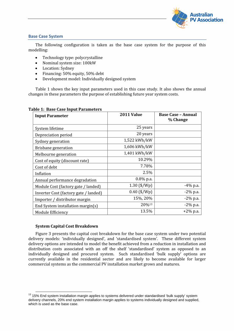
Figure 3: Base Case System (100kWp) Capital Cost Breakdown(Standardised System vs Individual Design) – excludes Solar Credits

Figure 3 shows that the (landed / factory gate) cost of PV modules and inverters nowrepresents under half the final system cost, with the rest represented by balance of systemelements along with the business channel costs of importers / distributors and installationcompanies. The difference between the standardised system and individually designed system(3.50 $/Wp vs 3.80 $/Wp) illustrates the potential for innovative and efficient delivery modelsto drive system cost reductions.

As the commercial system PV market is still immature relative to the residential PV market,we have chosen the higher cost individually designed system as the base case system forconsideration herein.

Grid Parity

‘Grid parity’ is the point at which the LCOE from PV falls at or below the cost of purchasingelectricity from the grid under standard electricity supply arrangements. Grid parity can beassessed in the following two ways:

On the basis of the price of grid electricity paid in the year of system installation; or

On the basis of the net present value of the electricity offset by the PV system overits life.

While comparing the LCOE from PV with the net present value of the electricity offset by thesystem over its lifetime may be an analogous comparison (apples with apples), it is more likelythat consumer decisions, and the rate of system deployment, will be driven by the price of gridelectricity paid in the year of system installation. In addition, a system payback period of lessthan the system life may well be required by business investors.

Figure 4 shows that, assessed on the basis of the net present value of the electricity offset bythe system over its life, the point of ‘grid parity’ has already been reached for base case systemslocated in Sydney and Brisbane, and is should be reached by 2012 for base case systems locatedin Melbourne.

When grid parity is assessed on the more conservative basis of the price of grid electricitypaid in the year of system installation, the point of ‘grid parity’ is reached by 2013 for a basecase system located in Sydney and Brisbane and 2015 for the same system located inMelbourne.

0

0.5

1

1.5

2

2.5

3

3.5

4

4.5

0

50,000

100,000

150,000

200,000

250,000

300,000

350,000

400,000

450,000

StandardisedSystem

Individual Design

Inst

alle

dC

ost

($/W

p)

20

11

$End System DeveloperMargin

Professional and ProjectCosts

Power Equipment Costs

Structural and Support Costs

Distributor Margin

Installation Costs

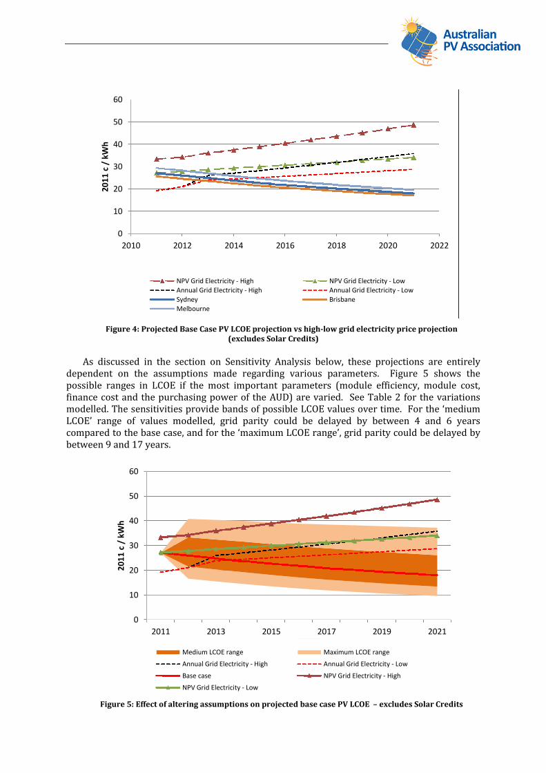
Figure 4: Projected Base Case PV LCOE projection vs high-low grid electricity price projection(excludes Solar Credits)

As discussed in the section on Sensitivity Analysis below, these projections are entirelydependent on the assumptions made regarding various parameters. Figure 5 shows thepossible ranges in LCOE if the most important parameters (module efficiency, module cost,finance cost and the purchasing power of the AUD) are varied. See Table 2 for the variationsmodelled. The sensitivities provide bands of possible LCOE values over time. For the ‘mediumLCOE’ range of values modelled, grid parity could be delayed by between 4 and 6 yearscompared to the base case, and for the ‘maximum LCOE range’, grid parity could be delayed bybetween 9 and 17 years.

Figure 5: Effect of altering assumptions on projected base case PV LCOE – excludes Solar Credits

0

10

20

30

40

50

60

2010 2012 2014 2016 2018 2020 2022

20

11

c/

kWh

NPV Grid Electricity - High NPV Grid Electricity - Low

Annual Grid Electricity - High Annual Grid Electricity - Low

Sydney Brisbane

Melbourne

0

10

20

30

40

50

60

2011 2013 2015 2017 2019 2021

20

11

c/

kWh

Medium LCOE range Maximum LCOE range


Base case NPV Grid Electricity - High

NPV Grid Electricity - Low

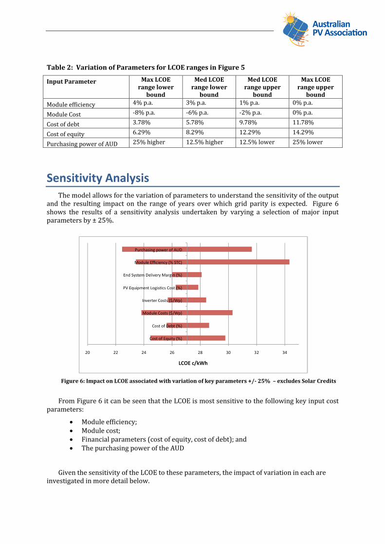
Table 2: Variation of Parameters for LCOE ranges in Figure 5

Input Parameter Max LCOErange lower

bound

Med LCOErange lower

bound

Med LCOErange upper

bound

Max LCOErange upper

bound

Module efficiency 4% p.a. 3% p.a. 1% p.a. 0% p.a.

Module Cost -8% p.a. -6% p.a. -2% p.a. 0% p.a.

Cost of debt 3.78% 5.78% 9.78% 11.78%

Cost of equity 6.29% 8.29% 12.29% 14.29%

Purchasing power of AUD 25% higher 12.5% higher 12.5% lower 25% lower

Sensitivity AnalysisThe model allows for the variation of parameters to understand the sensitivity of the output

and the resulting impact on the range of years over which grid parity is expected. Figure 6shows the results of a sensitivity analysis undertaken by varying a selection of major inputparameters by ± 25%.

Figure 6: Impact on LCOE associated with variation of key parameters +/- 25% – excludes Solar Credits

From Figure 6 it can be seen that the LCOE is most sensitive to the following key input costparameters:

Module efficiency; Module cost; Financial parameters (cost of equity, cost of debt); and The purchasing power of the AUD

Given the sensitivity of the LCOE to these parameters, the impact of variation in each areinvestigated in more detail below.

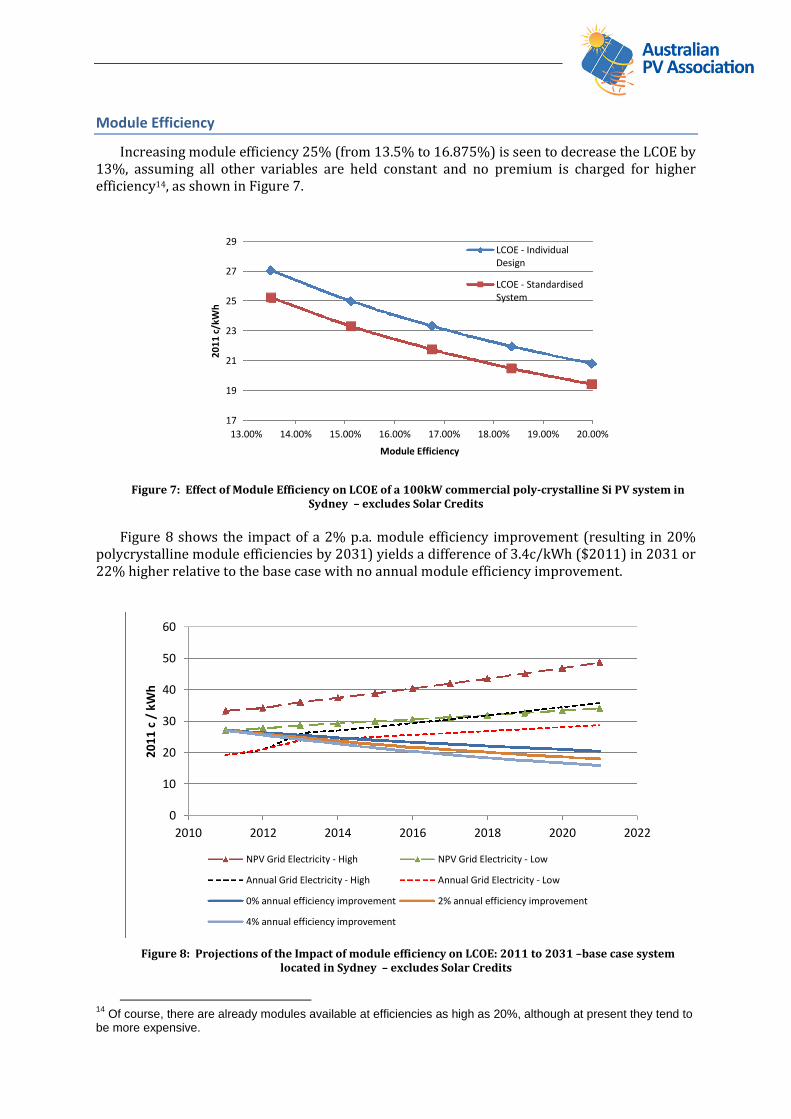
Module Efficiency

Increasing module efficiency 25% (from 13.5% to 16.875%) is seen to decrease the LCOE by13%, assuming all other variables are held constant and no premium is charged for higherefficiency14, as shown in Figure 7.

Figure 7: Effect of Module Efficiency on LCOE of a 100kW commercial poly-crystalline Si PV system inSydney – excludes Solar Credits

Figure 8 shows the impact of a 2% p.a. module efficiency improvement (resulting in 20%polycrystalline module efficiencies by 2031) yields a difference of 3.4c/kWh ($2011) in 2031 or22% higher relative to the base case with no annual module efficiency improvement.

Figure 8: Projections of the Impact of module efficiency on LCOE: 2011 to 2031 –base case systemlocated in Sydney – excludes Solar Credits

14Of course, there are already modules available at efficiencies as high as 20%, although at present they tend to

be more expensive.

17

19

21

23

25

27

29

13.00% 14.00% 15.00% 16.00% 17.00% 18.00% 19.00% 20.00%

20

11

c/kW

h

Module Efficiency

LCOE - IndividualDesign

LCOE - StandardisedSystem

0

10

20

30

40

50

60

2010 2012 2014 2016 2018 2020 2022

20

11

c/

kWh



0% annual efficiency improvement 2% annual efficiency improvement

4% annual efficiency improvement

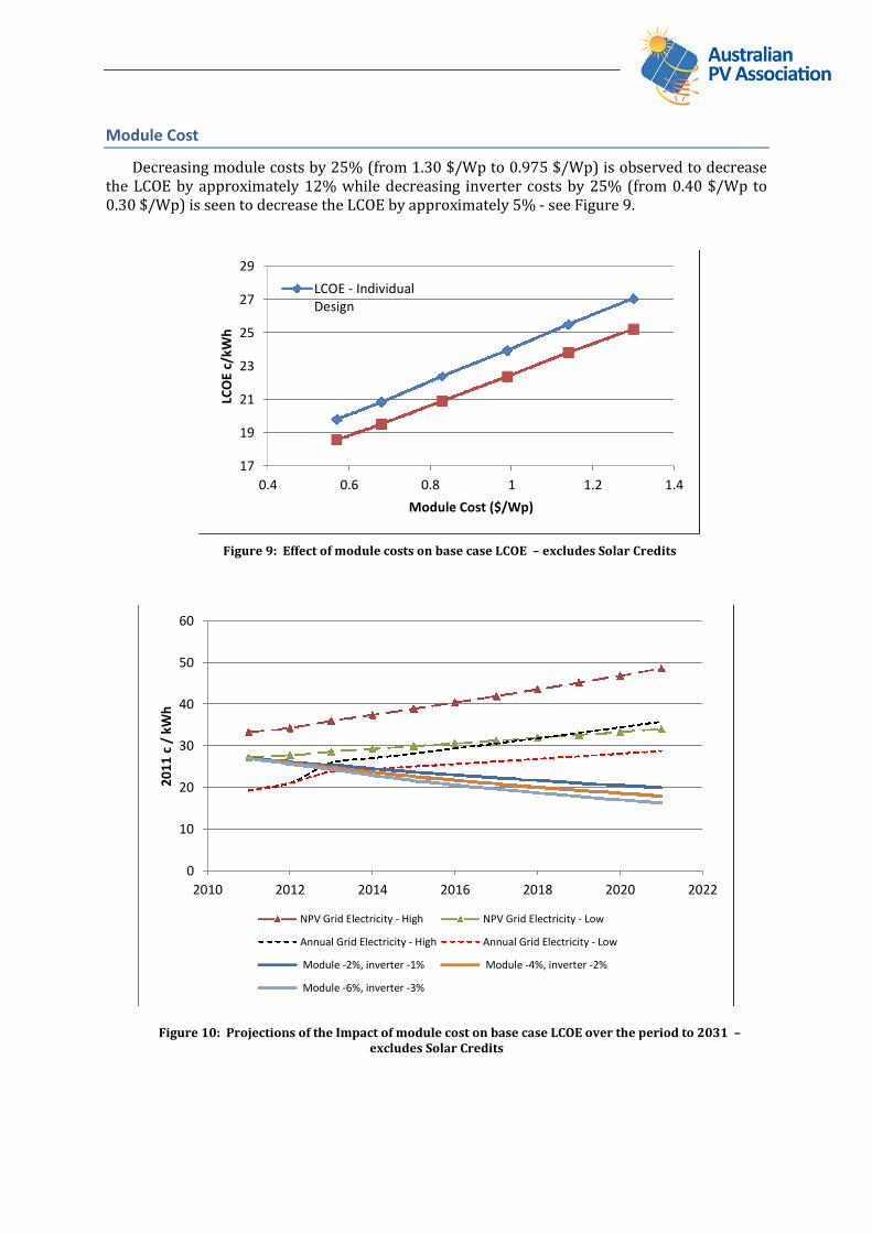
Module Cost

Decreasing module costs by 25% (from 1.30 $/Wp to 0.975 $/Wp) is observed to decreasethe LCOE by approximately 12% while decreasing inverter costs by 25% (from 0.40 $/Wp to0.30 $/Wp) is seen to decrease the LCOE by approximately 5% - see Figure 9.

Figure 9: Effect of module costs on base case LCOE – excludes Solar Credits

Figure 10: Projections of the Impact of module cost on base case LCOE over the period to 2031 –excludes Solar Credits

17

19

21

23

25

27

29

0.4 0.6 0.8 1 1.2 1.4

LCO

Ec/

kWh

Module Cost ($/Wp)

LCOE - IndividualDesign

0

10

20

30

40

50

60

2010 2012 2014 2016 2018 2020 2022

20

11

c/

kWh



Module -2%, inverter -1% Module -4%, inverter -2%

Module -6%, inverter -3%

Modules remain the single biggest element of the final system delivery cost. As such, theLCOE is observed to be sensitive to variation in module costs15. Figure 10 shows thatdecreasing 2011 $/Wp module costs from $1.30 to $0.57/Wp (as would occur between 2011and 2031 with a 4% p.a. reduction in module costs) decreases the LCOE by 37%, from 27c to20c/kWh ($2011).

Finance Costs

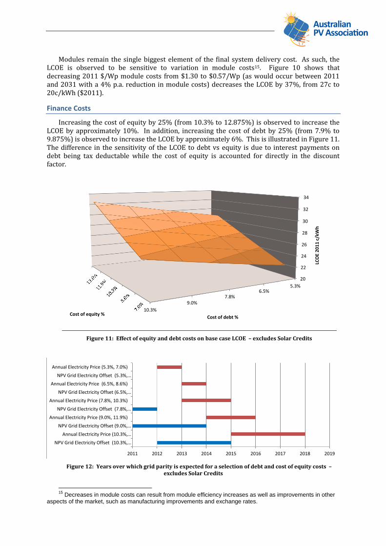
Increasing the cost of equity by 25% (from 10.3% to 12.875%) is observed to increase theLCOE by approximately 10%. In addition, increasing the cost of debt by 25% (from 7.9% to9.875%) is observed to increase the LCOE by approximately 6%. This is illustrated in Figure 11.The difference in the sensitivity of the LCOE to debt vs equity is due to interest payments ondebt being tax deductable while the cost of equity is accounted for directly in the discountfactor.

Figure 11: Effect of equity and debt costs on base case LCOE – excludes Solar Credits

Figure 12: Years over which grid parity is expected for a selection of debt and cost of equity costs –excludes Solar Credits

15Decreases in module costs can result from module efficiency increases as well as improvements in other

aspects of the market, such as manufacturing improvements and exchange rates.

5.3%6.5%

7.8%9.0%

10.3%

20

22

24

26

28

30

32

34

Cost of debt %LC

OE

20

11

c/kW

hCost of equity %

2011 2012 2013 2014 2015 2016 2017 2018 2019

NPV Grid Electricity Offset (10.3%,…

Annual Electricity Price (10.3%,…


Annual Electricity Price (9.0%, 11.9%)







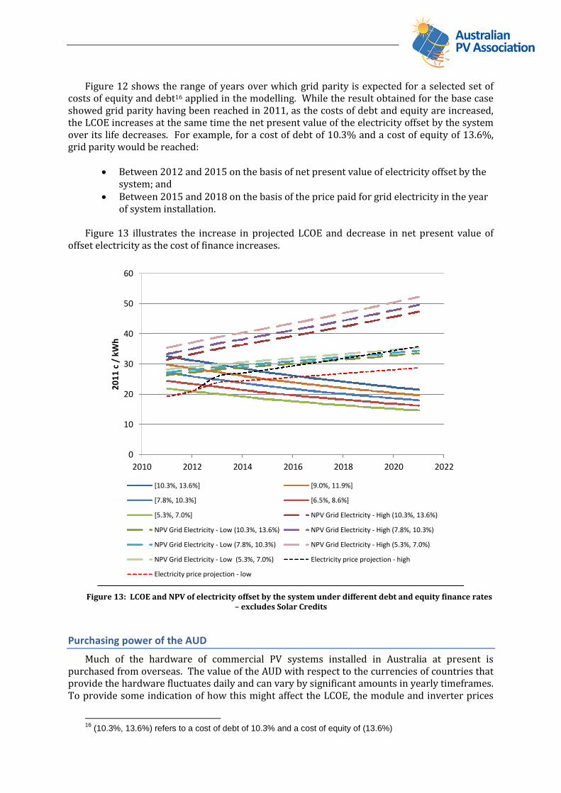
Figure 12 shows the range of years over which grid parity is expected for a selected set ofcosts of equity and debt16 applied in the modelling. While the result obtained for the base caseshowed grid parity having been reached in 2011, as the costs of debt and equity are increased,the LCOE increases at the same time the net present value of the electricity offset by the systemover its life decreases. For example, for a cost of debt of 10.3% and a cost of equity of 13.6%,grid parity would be reached:

Between 2012 and 2015 on the basis of net present value of electricity offset by thesystem; and

Between 2015 and 2018 on the basis of the price paid for grid electricity in the yearof system installation.

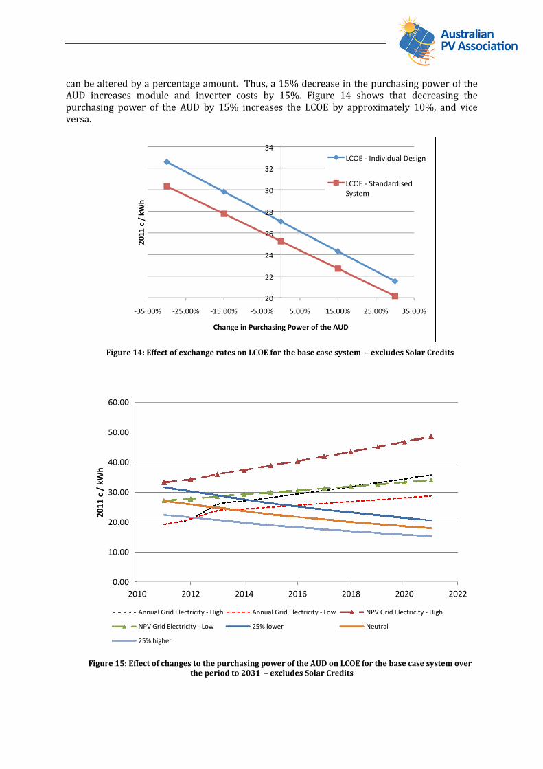
Figure 13 illustrates the increase in projected LCOE and decrease in net present value ofoffset electricity as the cost of finance increases.

Figure 13: LCOE and NPV of electricity offset by the system under different debt and equity finance rates– excludes Solar Credits

Purchasing power of the AUD

Much of the hardware of commercial PV systems installed in Australia at present ispurchased from overseas. The value of the AUD with respect to the currencies of countries thatprovide the hardware fluctuates daily and can vary by significant amounts in yearly timeframes.To provide some indication of how this might affect the LCOE, the module and inverter prices

16(10.3%, 13.6%) refers to a cost of debt of 10.3% and a cost of equity of (13.6%)

0

10

20

30

40

50

60

2010 2012 2014 2016 2018 2020 2022

20

11

c/

kWh

[10.3%, 13.6%] [9.0%, 11.9%]

[7.8%, 10.3%] [6.5%, 8.6%]

[5.3%, 7.0%] NPV Grid Electricity - High (10.3%, 13.6%)

NPV Grid Electricity - Low (10.3%, 13.6%) NPV Grid Electricity - High (7.8%, 10.3%)

NPV Grid Electricity - Low (7.8%, 10.3%) NPV Grid Electricity - High (5.3%, 7.0%)

NPV Grid Electricity - Low (5.3%, 7.0%) Electricity price projection - high

Electricity price projection - low

can be altered by a percentage amount. Thus, a 15% decrease in the purchasing power of theAUD increases module and inverter costs by 15%. Figure 14 shows that decreasing thepurchasing power of the AUD by 15% increases the LCOE by approximately 10%, and viceversa.

Figure 14: Effect of exchange rates on LCOE for the base case system – excludes Solar Credits

Figure 15: Effect of changes to the purchasing power of the AUD on LCOE for the base case system overthe period to 2031 – excludes Solar Credits

0.00

10.00

20.00

30.00

40.00

50.00

60.00

2010 2012 2014 2016 2018 2020 2022

20

11

c/

kWh

Annual Grid Electricity - High Annual Grid Electricity - Low NPV Grid Electricity - High

NPV Grid Electricity - Low 25% lower Neutral

25% higher

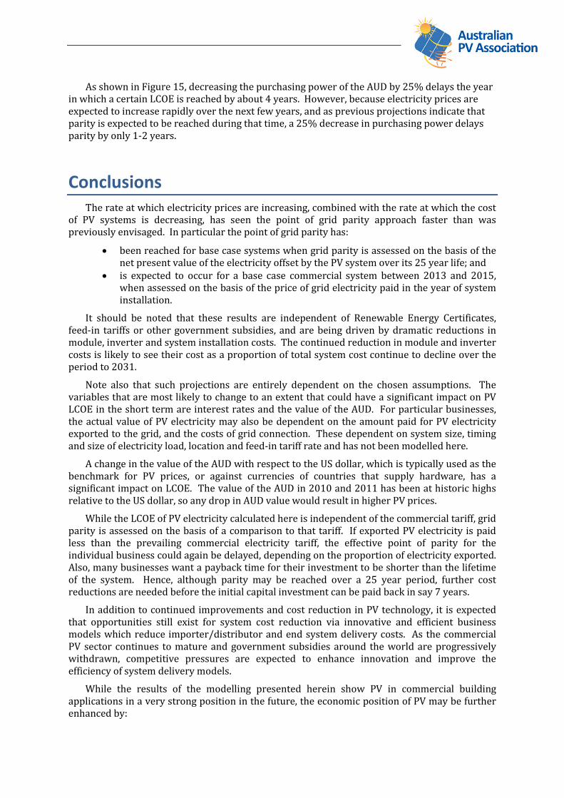
As shown in Figure 15, decreasing the purchasing power of the AUD by 25% delays the yearin which a certain LCOE is reached by about 4 years. However, because electricity prices areexpected to increase rapidly over the next few years, and as previous projections indicate thatparity is expected to be reached during that time, a 25% decrease in purchasing power delaysparity by only 1-2 years.

ConclusionsThe rate at which electricity prices are increasing, combined with the rate at which the cost

of PV systems is decreasing, has seen the point of grid parity approach faster than waspreviously envisaged. In particular the point of grid parity has:

been reached for base case systems when grid parity is assessed on the basis of thenet present value of the electricity offset by the PV system over its 25 year life; and

is expected to occur for a base case commercial system between 2013 and 2015,when assessed on the basis of the price of grid electricity paid in the year of systeminstallation.

It should be noted that these results are independent of Renewable Energy Certificates,feed-in tariffs or other government subsidies, and are being driven by dramatic reductions inmodule, inverter and system installation costs. The continued reduction in module and invertercosts is likely to see their cost as a proportion of total system cost continue to decline over theperiod to 2031.

Note also that such projections are entirely dependent on the chosen assumptions. Thevariables that are most likely to change to an extent that could have a significant impact on PVLCOE in the short term are interest rates and the value of the AUD. For particular businesses,the actual value of PV electricity may also be dependent on the amount paid for PV electricityexported to the grid, and the costs of grid connection. These dependent on system size, timingand size of electricity load, location and feed-in tariff rate and has not been modelled here.

A change in the value of the AUD with respect to the US dollar, which is typically used as thebenchmark for PV prices, or against currencies of countries that supply hardware, has asignificant impact on LCOE. The value of the AUD in 2010 and 2011 has been at historic highsrelative to the US dollar, so any drop in AUD value would result in higher PV prices.

While the LCOE of PV electricity calculated here is independent of the commercial tariff, gridparity is assessed on the basis of a comparison to that tariff. If exported PV electricity is paidless than the prevailing commercial electricity tariff, the effective point of parity for theindividual business could again be delayed, depending on the proportion of electricity exported.Also, many businesses want a payback time for their investment to be shorter than the lifetimeof the system. Hence, although parity may be reached over a 25 year period, further costreductions are needed before the initial capital investment can be paid back in say 7 years.

In addition to continued improvements and cost reduction in PV technology, it is expectedthat opportunities still exist for system cost reduction via innovative and efficient businessmodels which reduce importer/distributor and end system delivery costs. As the commercialPV sector continues to mature and government subsidies around the world are progressivelywithdrawn, competitive pressures are expected to enhance innovation and improve theefficiency of system delivery models.

While the results of the modelling presented herein show PV in commercial buildingapplications in a very strong position in the future, the economic position of PV may be furtherenhanced by:

- Reducing grid connection costs by connecting behind the meter in locations where theminimum load is greater than the PV system’s peak output, and by developing standardgrid connection procedures for systems which export power

- promoting the installation of larger systems (that are still small enough to connect to thedistribution network)

- promoting the use of ‘standardised’ systems, where the supply and installation processis streamlined and

- reducing module cost, which can occur through module efficiency improvements as wellas through other activities such as improvements to manufacturing processes

- likely reductions in inverter and other balance of system costs have a relatively smalleffect, but of course should not be overlooked as part of overall cost reductions.

Uses for the Model

The model could usefully be applied to a range of analyses, including:

Assessing the impacts of:

State feed-in tariffs and Commonwealth support programs e.g. RenewableEnergy Certificates

alternative wholesale and retail electricity price projections

changes in Australian dollar exchange rates

possible tax incentives for the commercial sector.

Modelling specific installations, systems and locations

Adding an upfront interface to more detailed PV output models and solar radiationdatabases, so that half hourly analyses can be undertaken of:

Time of use tariffs and values

Demand reduction values

Building integrated PV potential

Different PV orientations.

Given the rapid rate of development in the PV sector, annual updates of the model defaultvalues should be undertaken.

Next Steps

The model outputs highlight the key requirements for PV to be cost effective against gridelectricity for commercial customers, but they also point to a range of wider issues, in additionto technical changes to the grid, which will need to be addressed in order to set appropriateregulatory frameworks for high PV penetration levels. These include:

Understanding how the fixed and marginal costs of electricity (wholesale, networks &retail) paid by retailers are transferred through to commercial consumers and what thismeans for distributed generation.

Understanding the costs and benefits to retailers if PV electricity is allowed to beexported to the grid – for instance, do network standing charges & demand charges that

commercial customers pay secure equitable access to marginal retail prices as rewardfor any exported solar electricity?

Assessing whether net metering fairly reflects network and energy costs and should bethe long term price setting default for distributed generation in a sustainable marketwithout specific technology based policy intervention

Reviewing non cost-based barriers to solar electricity in the Australian electricitymarkets, including ability of commercial PV generating plants to connect to the grid, toexport power and the relevance of current market rules for distributed generation.

Documents

Commercial Sector Modelling of PV and Electricity Prices ...apvi.org.au/.../Commercial-Sector-Modelling-of-PV-and-Electricity... · Modelling of PV and Electricity ... generated by