Embed Size (px)
Citation preview

MODELLING DETERMINANTS OF POVERTY IN ERITREA: A
NEW APPROACH By Eyob Fissuh+ and Mark Harris*
________________________________________________________________
Abstract This paper uses DOGEV model for modelling determinates of poverty in Eritrea by employing Eritrean Household Income and Expenditure Survey 1996/97 data. Education impacts welfare differently across poverty categories and there are pockets of poverty in the educated population sub group. Effect of household size is not the same across poverty categories. Contrary to the evidence in the literature the relationship between age and probability of being poor was found to be convex to the origin. Regional unemployment was found to be positively associated with poverty. Remittances, house ownership and access to sewage and sanitation facilities were found to be highly negatively related to poverty. This paper also finds out that there is captivity in poverty category and a significant correlation between poverty orderings which renders usage of standard multinomial/ordered logit in poverty analysis less defensible. ________________________________________________________________________________
Key Words: Poverty, Eritrea, Dogev, Dogit and Ogev.
JEL classification: C3, I32, O18.
________________________________________________________________________________
INTRODUCTION Poverty is widespread in Eritrea. This has been one of the stylized facts of sub-
Saharan Africa (Schoumaker, 2004). Regrettably, it has got the least attention and
consequently there has not been a full-fledged poverty study in Eritrea to date. The
income poverty measures presented in most cases are based on a Rapid Appraisal
Survey conducted in 1993/94. Because the survey was conducted so soon after the
war, when conditions were still unsettled, the results must be considered preliminary.
About 50 percent of households in Eritrea were estimated to be poor in 1993–94, i.e.,
to not have sufficient income or endowments to consume a minimum requirement of
2000 calories per capita per day, plus a few other essential non food commodities
such as clothing and housing. In that year because of drought, 70-80 percent of the
households received food aid; without it, 69 percent of the population would have
been unable to consume the minimum basket of food and other essential commodities
(World bank, 1996).
+ Department of Econometrics and Business Statistics, Monash University, Clayton, Victoria 3800, Australia. *Department of Econometrics and Business Statistics, Monash University, Clayton, Victoria 3800, Australia. Address for correspondence [email protected]
1

LITERATURE REVIEW The art of modelling poverty seem to be preoccupied in getting the best criteria for
the judgment of the poverty status of individuals. Rouband and Razafindrakoto(2003)
assert that there is correlation of the objective and subjective poverty measures and
further argue that the various forms of poverty are not reducible one against the other.
Apart from being obsessed with monetary approach for measuring poverty there has
been a growing literature which tries to come up with an index of multidimensional
poverty facet1. However there is little conclusion so far and as Kanbur and Squire
(1999) argue there is no material difference in the number of poor identified as poor
by employing different approaches. This seems to be convincing for at least the hard
core poor where they are poor are in every dimension. Moreover after comparing
different definitions of poverty and their implication to poverty modelling Rouband
and Razafindrakoto (2003) argue that the traditional approach of monetary approach
to measurement of poverty seems justified as it is the one most correlated with the
other subjective measures2. The devil is not on the usage of money metric unit for the
determination of absolute poverty line rather on the mechanism employed for the
derivation of such a line (Ravallion, 1996).The debate on the definition and
measurement of poverty is really far from settled (see Ravallion, 1996 and Laderchi,
R.C. et al, 20033).
The unavailability of any poverty analysis in Eritrea and rigorous attempt to define
and measure absolute poverty line constrains the choice to monetary approach
developed by the World Bank. According to the World Bank quick appraisal group,
absolute poverty line is “the minimum cash and non cash expenditure needed to be
made by a person or household in order to be able to consume a minimum number of
calories (food) plus a small number of essential non food items such as housing and
1 See Bourguignon and Chakravarty(2003) for the treatment of poverty measurement from multidimensional perspective. 2 However, they assert that it is sufficient and would be good if it could be augmented by non monetary. Of course, ultimately any subjective approach will converge to the monetary approach, at least when it comes to practice. The capacity of the welfare ratio in representing the money metric unit of utility is a function of the institutional setting and the definition of welfare which is variant with time and spatial space. 3 Ravallion (1996) comments on the modelling and measurement of poverty with reference to their repercussion to policy guidance. Laderchi, R.C. et al, 2003 give detailed discussion of the implication the different definitions of poverty to the measurement of poverty.
2

closing” (World bank, 1996:5). The World Bank group also calculate poverty lines
with and with out food aid, original poverty line minus the amount of food aid
received by a household4. Using this definition they calculate poverty lines by region
and at national level. With out going deep into the philosophy of this argument we
will adopt what was suggested by the World Bank.
There are basically two approaches in modelling determinants of poverty. The first
approach5 is the employment of consumption expenditure per adult equivalent and
regress it against potential explanatory variables (Geda et al, 2001). Using this
approach Arneberg and Pederson (2001) report that household characteristics and
education are the main factors which affect living standard in Eritrea. However, they
treat education as a linear and continuous variable. Moreover they find out that
transfer payment from relatives abroad is a significant contributor to the welfare of a
society. From their analysis they conclude that education is the most important factor
for the way out of poverty. However, their approach suffers from the common
problems of consumption as being indicator of welfare and the assumption that
consumption of the poor and non poor are both determined by the same process
(Okwi, 1999). The second approach is to directly model poverty by employing a
discrete choice model.
The practice of discrete choice models in the analysis of determinants of poverty has
been popular approach6 (for instance, Fafack(2002) for Burkian’faso, Kabubuo-
Mariara (2002) for Kenya; Amuedo_Dorantes(2004) for Chile; Grootaert(1997) for
Cote D’voire; Geda et al(2001) for Kenya; Charlette-Gueard and Mesple-Somps
(2001) for Cote d`voire , Goaed and Ghazouani(2001) for Tunisia; Roubaud and
Razafindrakoto ,2003). The analysis then proceeds by employing binary logit or
probit model to estimate the probability of a household being poor conditional up on
4 See World Bank (1996) for details of calculations. In addition the International poverty line one USD per day was employed but they fairly give almost the same classification which does not significantly change the multivariate analysis. 5 This approach works by regressing consumption expenditure (in log terms) on the household, community and common characteristics which are supposed to determine household welfare, for example Glewwe(1990), Muller(1999) and Canagarajah and Portner(2003). This approach rests on a heroic assumption that higher expenditure implies higher utility and vice versa. 6 Another approach is to combine these two approaches by using multinomial logit selection model to analyse the determinants of living standards (see Mckay and Coloube ,1996 for Muritania). This approach is not yet common though.
3

some characteristics. In some cases also the households are divided into three
categories: absolute poor, poor and non poor and then employ ordered logit or ordered
logit model to identify the factors which affect the probability a household being poor
conditional up on set of characteristics. In this study we buy the latter approach to
divide the population into poverty categories in Eritrea. However we employ DOGEV
model a class of extreme value distributions which is proposed by Fry and Harris
(2002).
The discrete choice model has a number of attractive features in comparison to the
expenditure approach. The expenditure approach unlike the discrete choice models
does not give probabilistic estimates for the classification of the sample into different
poverty categories. In a sense we can not make probability statements about the effect
of the variables in the poverty status of our economic agents. The consumption
approach assumes that consumption expenditures are negatively correlated with
absolute poverty at all expenditure levels. By the same logic, factors which increase
expenditure reduce poverty. However, this is not always the case. For instance
increasing consumption expenditure for individuals above the poverty line will not
affect the poverty level. On the other hand in our discrete choice model we may allow
the effects of independent variables to vary across poverty categories. Lastly our
approach tries to capture any heterogeneity between the moderate poor, non poor and
absolute poor with a possibility of weak test for of any captivity or “poverty trap” in
static sense in each group. This is not possible in the expenditure function approach.
However this approach of modelling poverty is not with out flaws. The prime concern
is that there is loss of information when we create categories of poverty status by the
level of consumption expenditure or income. Secondly the fact that all those who are
above the poverty line are intentionally considered to be homogenous or identical may
not be tolerable (Jollife and Datt, 1999).This may imply superimposing censorship
into the data set. Thirdly there is arbitrariness in the setting of the absolute poverty
line. This necessitates the usage of some dominance analysis to check the robustness
of the poverty line that we employ. Lastly we need to assume about the distribution of
our non linear model. The last act is a matter of econometric practice, though.
4

Moreover there are two fundamental problems built in to the underlying assumption
of employing standard ordered logit and Multinomial logit model which usually get
little attention in such applications. With regards to former, the ordered logit/probit
model, it is restrictive because it makes the parameters to be the same across groups.
Ordered logit or ordered logit models necessitate the specification of a single latent
variable in linear function. Consequently these models do not have the flexibility of
MNL or multivariate probit (Small, 1987). Ravallion (1996) argues that although
employment of binary response models as opposed to the multinomial logit model are
redundant , it is not unjustified to attempt estimating set of regression functions by
letting the impact of the explanatory variables to vary across the distribution poverty,
poverty categories, as in multinomial logit model. This practice implicitly relaxes the
first order dominance assumption implicit in the employment of a single parameter for
each explanatory variable throughout the distribution of welfare ratio. With regards
to the latter convenience is bought at the expense of heroic assumption, Independence
of Irrelevant Alternatives (IIA), which does not stand in reality. IIA states that the
odds ratio kjPP
ik
ij ≠, is independent of the choice set. That is for any choice sets
and such that and , and for any alternatives i and in both and
we have
1C 2C nCC ⊆1 nCC ⊆2 j 1C
2C
)/()/(
)/()/(
2
2
1
1
CjPCiP
CjPCiP
= 1
This assumption is in most instances implausible. Moreover Fry and Harris (1996)
test for IIA and report that it has very poor power properties. There have been many
suggestions in increasing the flexibility of the extreme value models so as to take into
account of these fundamental problems (Koppelman and Sethi, 2000). The novelty of
our methodology is that we employ alternative model which remedies these vital
flaws. Unlike previous studies we employ a DOGEV model which allows for the
parameters of explanatory variables to vary across poverty categories, as in the
ordinary MNL and possible correlation between adjacent categories where the aim is
mainly comparing the category specific error terms as in Diamond et at. (1990).
5

MODEL SPECIFICATION Since at the heart of any poverty modelling exercise is identification of main factors
which dictate poverty outcomes, we want to ask the following question: what is the
probability that a family with particular identifiable characteristics will be found in a
specific poverty stratum. This probabilistic framework for the study of poverty will
assume that the real poverty status of the house holds is not observable or is not
correctly indicated by the welfare ratio7. Following Fry and Harris (2002) we suggest
DOGEV model 8 which nests the DOGIT and OGEV models as its variant.
The first feature of DOGEV, which is borrowed from Dogit, is the introduction of
choice specific parameters rendering DOGEV to be flexible with additional
parameters, jθ and needs discussion so as to finesse the issue. Following Gaudry and
Dagenais(1979) the Dogit discrete choice model takes the form:
( )∑∑∑
==
=
+
+= J
k ikJ
k k
J
k ijjijDOGITij
V
VVP
11
1
)exp(1
)exp()exp(
θ
θ or
( )MNL
ijJ
k kJ
k k
jDOGITij PP ×
++
+=
∑∑ == 111
1
1 θθ
θ 2
where is the probability of individual choosing alternative . ijP thi j
jθ is the parameter associated with alternative; thj 0≥jθ
is the function of k independent attributes of the alternative , i.e, ijV ijkX thj
jiij xV β'=
7 One can also argue that these observed ratio of consumption to absolute level of poverty is less reliable and can only be trusted within a margin and hence the true poverty status of households is not correctly explained by these figures. Given the arbitrariness of poverty line also this division of poverty status into categories is not unreasonable. 8 Although most of class of logit models are usually derived from a process of utility maximization, which is not observable behaviour, over discrete choices this approach abstains from a process of utility maximization perspective, although one can argue that there is an element of choice for being poor. For instance one can postulate that people will struggle to get out of poverty by going to school and may also choose the way of living and choice in which poverty strata to fall in. This is not to claim that people have readily available choices to fall under different poverty strata though. There may be a huge chunk of element which hinders individuals from choosing among potential alternatives. It is also fair to assume that any rational household will not choose to be in poverty. Although the decisions made by the family may lead to poverty and ultimately the household is choosing poverty. At best we can argue poverty is a manifestation of household choice. However in this paper the choice of multinomial probability distribution is purely pragmatic.
6

∑ =
= J
k ik
ijMNLij
V
VP
1)exp(
)exp(
As it is clear from the above equation we can see that any two alternatives are not
independent except in the special cases where all jθ are equal to zero where in that
case the model reduces to the ordinary MNL model. Given in this model that the
probabilities of any two alternatives are affected by other alternatives is major
behavioural departure from the Multinominal Logit model (Gaudry, 1980). This θ can
be interpreted as a measure of captivity in the poverty category9. These jθ can also be
made to be a function of some observed heterogeneity (Fry and Harris, 2001).
However in this paper we will not do that. Rather we will assume that these
parameters will capture the heterogeneity across the different poverty status but
constant across households10.
These parameters can be interpreted as indication of heterogeneity of the outcome as
opposed to individual heterogeneity. Moreover these parameters may indicate the
individual heterogeneity which falls across each category. For example those who are
in the absolute poverty category could not get out of that poverty because of physical
disability which is not accounted by any of the explanatory variables in our model
may be captured by jθ . Generally this approach of modelling is very promising the
fact that we have many war disabled veterans and elderly people who may be stuck in
a poverty category. For instance as Deaton (1997) indicates malnutrition could impair
productivity and thereby keep people in a poverty trap. Our model has a potential for
capturing such imprisonment of household in a poverty jail because of some
unobserved variables in the welfare categories.
The second advantage of DOGEV model is borrowed from OGEV- due to
Small(1987). This model tries to mock-up a qualitative limited dependent variable
with natural ordering and strong heterogeneity of the realized outcomes (Fry and
Harris, 2002). It allows for a flexible covariance pattern between alternatives as
9 In the analysis of demand this is interpreted as the income effects and its role is reducing the own price elasticity of logit estimates and increases the cross partial elasticity (Gaudry, 1980). 10 see Fry et al(2002) for parameterized DOGEV model . Borderly(1990) argues that the Dogit model is useful with out perfect captivity.
7

opposed to the IIA of MNL model. This paper contends that there may be correlation
among the unobserved traits of several alternatives facing a given sample member in
the poverty categories. In the terminology of Small (1987), we introduce stochastic
correlation between choices of close proximity. This correlation is a variant of the
moving average which fades out with distance between the alternatives, say and
and in addition we assume following Small (1987) that it will be zero if .
The standard OGEV probabilities are given by
j
k 2][ >− kj
( ) ( )( )( ( ) ( ) )[ ]
( ) ( )( ) 11
11
111
1
1
11
11
1
expexp
expexpexpexp
)exp(
−
+−−
−−−
−
+
=−
−−
−
++
+×+
=∑
ρ
ρρ
ρρ
ρρρρ
ρ
ijij
ijijJ
r irir
ijOGEVij
VV
VVVV
VP
3
With the convention that ( ) ( ) 0expexp 11
01 == +
−−iJi VV ρρ and 10 << ρ .
The correlation parameter ρ is an inverse measure of the correlation between the
neighbouring outcomes. It does not have closed formula in this specification though.
In the limit as ρ approaches to 1, the above OGEV model collapses to an ordinary
MNL model. Thus we can set 1=ρ as a hypothesis to test OGEV versus MNL. That
is to say we are implicitly checking if there is ordering in our choice set11.
Following DOGEV model proposed by Fry and Harris (2002), the paper argues that
poverty status ordering is based on an underling distribution of welfare ratio. In
addition the dependent variable, the poverty ordering is the representation of the
underlying continuous variable of poverty. The fact that we employ poverty line to
create a jump or discontinuity in the poverty status of households, we may expect
high probability of correlation between poverty outcomes12. The DOGEV discrete
choice model takes the form:
OGEVijM
k kM
k k
jDOGEVij PP ×
++
+=
∑∑ == 111
11 θθ
θ 4
where we have the nested models
11 Small (1987) shows that as 0=ρ the cumulative distribution function collapses to one and he argues that it is still in line with the random utility maximization. 12 Employment of absolute poverty line implies that there is a discontinuity in the distribution of welfare (Deaton, 1997).
8

OGEV: 10,0...1 ≤<=== ρθθ M
DOGIT: 1=ρ at least one Jjj ,...,1,0 =>θ
MNL: 1,0...1 ==== ρθθ M
The latter two do not incorporate any ordering between outcomes. However the
former does. The capability of modelling an ordinal data in such a way that it captures
any captivity makes DOGEV more attractive. The above nested models can be tested
by the classical testing mechanisms but now with one sided test.
As in the usual binary mode we are not interested inβ . We are interested in the
marginal effects of changes in the regressors. However because of the complications
in the computation of these marginal effects we will report the change in the
probabilities as a result of change in the variables of interest throughout this paper,
which are essentially marginal effects in any case.
To estimate the DOGEV model we employ maximum likelihood technique. By
employing an indicator function 1=ijh if an individual chooses alternative i j or 0
otherwise. The log-likelihood function is given by
∑∑= =
=J
j
N
i
DOGEVijij PhL
1 1
ln)(φ where ( )[ ]ρθβφ ,','' jvec= and given by equation
4. Likewise the log likelihood functions for the nested models could be written down
simply by imposing restrictions to this general log likelihood function.
DOGEVijP
DATA The data are drawn from the Eritrean Household Income and Expenditure Survey
(EHIES), an urban survey that was conducted in the large towns of Eritrea in 1996.
The survey was conducted from July to September 1996 in four rounds so as to
incorporate seasonal variations in data collection It was designed to be able to report
separately from five main geographical reporting domains corresponding to the three
large towns, the Highlands and the Western Lowlands. The National Statistics Office
selected a sample size of 5,061 households. Of the selected total 5,061 households,
the surveyors were able to include 4,644 households in the data. The non-response
rate was very low. However, the data do not include all the variables needed for the
9

analysis, and the data set also has many missing observations and some outliers.
These problems are omnipresent in most developing countries (Deaton, 1997). As a
result, the data had to be cleaned for the missing information and anomalies and the
effective sample size was 3712 households. The absence of any operational sampling
framework in the country necessitated complete mapping and listing of all households
in all towns except in one town, Keren. The sampling method employed was one-
stage stratified sampling in all towns. Simple random sampling was used to choose
households from the selected clusters.
DESCRIPTIVE ANALYSIS
In this section we give descriptive analysis of the data used for analysis. We first
define our dependent variable with the dependent variable in our analysis. The
welfare ratio ( was derived by dividing expenditure per capita adjusted for
household size by respective regional poverty line. In the second stage each
household is assigned to poverty categories as per the following: absolute poverty
if ; moderate poverty: if
)iy
75.0<iy 25.175.0 ≤< iy and non poor if 25.1>iy .
Table 1.Distribution of poverty by welfare index
Poverty category Total Non poor Moderate Poor Absolute poor Frequency 1,108 1,433 1,171 3,712 Percentage 29.85 38.6 31.55 100
Source: Authors calculation from EHIES 1996/97. Note: As a robustness check we also employed the International poverty line suggested by World Bank but they give similar classification; with 31 35 and 34 percent being in absolute poverty, moderate poverty and non poor category.
Table 1 above clearly shows that 68.5 % of our sample dwells in poverty with 30
percent in absolute poverty and 38.5 percent in moderate poverty. Eventhough strictly
speaking this is not a measure of poverty index it is very close to the World Bank’s
head count index which is reported to be about 69 percent (World bank, 1996).
Poverty is not evenly distributed across different regions of Eritrea. At regional level
there are various characteristics that might correlate with poverty. The relationship of
these factors to poverty is of course a function of space and time. However generally
there a convention among development economists those areas with low resource
10

base and isolated from the main markets because of infrastructure and other facilities
are supposed to be more poverty socked than the urban areas in the core or around
Distribution of Poverty by town
0.010.020.030.040.050.060.070.080.090.0
adike
ih
akurd
et
asmar
a
assa
b
barentu
dece
mhare
ghind
a
keren
massa
wa
mende
fera
nakfa
tesse
ney
Town
perc
enta
ge fr
eque
ncy
012
Source: Authors calculation from EHIES 1996/97. Note: 0= Non poor. 1= Moderate poor. 2=Absolute poor. Figure 1 harbour. There is remarkable difference in terms of weather, level of development and
population distribution among urban areas. Figure 1 above clearly shows that majority
of the extreme poor are found in Adikeih, Keren and Nakfa. This may be explained by
the regional unemployment rate being the highest in Adikeih, 20% followed by Keren
18 %. Moreover the disparities may be explained by the inadequate public services
and weak communications and infrastructures as well as underdeveloped markets in
these periphery towns.
Schooling and Poverty
010203040506070
No formal education Basic Education Secondary Above secondary
Schooling
%fre
quen
cy Non poor
Moderate Poor
Absolute poor
Source: Authors calculation from EHIES 1996/97 Note: Basic education= grade 1-7. Secondary =grade 8-12. Above secondary= Grade >=12 Figure 2
Development thinkers and economists has long been busy postulating a positive
association between schooling and economic wellbeing. Figure 2 summarizes the
11

distribution of poverty across different educational attainments of household head.
Figure 2 shows that there is negative association between poverty and schooling.
Specifically 77% of the households with no formal education dwell in poverty among
which 41 percent being in the absolute poverty. While the distribution of absolute
poverty decreases with an increase in education level, the number of non poor
increases with increases in years of schooling completed. As far as the distribution of
moderate poor is concerned figure 2 suggests that it marginally increases until
elementary school and thereafter decreases slightly with increases in levels of
schooling completed. In light of these this paper employs dummy variables for the
different levels of education I the multivariate analysis.
Remittances from relatives within Eritrea or abroad are good indicators of poverty in
Eritrea Arneberg and Pederson (2001). However remittance is not evenly distributed.
Distribution of remittances mainly from relatives in Diaspora is inversely related to
poverty. Figure 3 shows that both remittances from relatives with in Eritrea and from
abroad are higher for the non poor households than poor household. In addition the
moderate poor household gets a slightly higher amount of remittance than the absolute
poor.13
Remmitance and poverty
0
500
1000
1500
2000
Absolute poor Moderate poor non poor
poverty status
aver
age
rem
mita
nce
TP-Local
TP-Abroad
Source: Authors calculation from EHIES 1996/97. Figure 3
The number of employed persons per household is a good gauge of poverty. It is
expected to be positively associated with poverty. The reasoning is straight forward,
more persons working implies more income coming to the household and 13 It is estimated that about one third of the population of Eritrea is in Diaspora.
12

Distribution of number of employed persons by poverty group
00.20.40.60.8
11.21.4
0 1 2Poverty group
NUmbe
r of e
mploy
ed per
cap
ita
Employed average
Source: Authors calculation from EHIES 1996/97. Figure 4
hence improvement in welfare. Figure 4 conforms to a priori expectation. On the
average the non poor people have higher number of people employed than both
moderate poor and absolute poor category. It is to be noted also that the number of
employed persons in moderately poor household is higher than those in the absolute
poverty.
In summary the above preliminary investigation suggests the significance of
demographic variables, human capital indicators, number of employment present,
regional unemployment, locality of residence and the availability of remittance from
abroad and home as determinants of poverty in Eritrea. However as it turn out to be
the above univariate analysis may not uncover some of the underlying relationships
which need to be seen in isolation. The next section presents multivariate analysis of
the above relationships by controlling some other underlying observed and
unobserved characterises. The model to be employed was developed in the previous
section.
EMPIRICAL RESULTS This section presents the estimated DOGEV model. Model discussed in the previous
section was estimated using poverty index as a dependent variable and explanatory
variables: demographic variables, community variables, labour force variables,
remittance, schooling, access to social services by controlling for regional differences.
13

The preferred model is DOGEV but we also report the results of ordered logit for
comparison purpose. Table 2 and 3 report DOGEV and ordered logit models.
Before presenting discussion of the coefficients it is worth discoursing the captivity
parameters and correlation between neighbouring outcomes, on which the ultimate
legitimacy of employing GODEV lies. With regards to the latter, as was explained in
the model development section, following Small (1978) the relevant test for the
ordering is a null of 1=ρ . According to table 2 the computed test statistic is big
enough to allow us reject the null hypothesis in favour of the alternative at less than
1% level. With regards to the former table 4 indicates that 1θ and 2θ are significantly
different from zero at 1% level of significance. However the captivity parameter for
the first category 0θ was not significantly different from zero as per our expectation,
because we would not expect any captivity in the non poor category. Our model was
estimated by imposing such an a priori restriction.
As far as the size of the captivity parameters is concerned it can be seen from their
contribution towards the total probability of observing a certain household being in a
poverty category, ∑ =
+M
k k
j
11 θ
θ. In most instances the contribution of the captivity
element towards the total predicted probabilities are of significant in size. It was
found out that the contribution of 1θ and 2θ towards the total predicted probabilities
on the average were 11 and 6 percent respectively. It is to be noted that the captivity
parameters are constant across individuals and hence their contribution towards each
individual variable can simply be found by dividing to the total probabilities
associated with each outcome at given values of the selected variables. The larger the
total probabilities as the explanatory variable change the smaller the contribution of
the captivity elements and vis-versa (see Table 3 in Appendix).
The captivity parameters may be explained by what characterizes deprivation,
vulnerability (high risk and low capacity to cope), and powerlessness (Lipton and
Ravallion, 1995; Sen, 1999). These characteristics weaken people's sense of well-
being. Poverty can be chronic or transient, but transient poverty, if acute, can trap
succeeding generations. According to our results the fact that the captivity element for
14

Table 2 DOGEV model: dependent variable poverty Moderate Poor Absolute poor
Variables Coefficient Standard Error
Coefficient
Standard Error
CONSTANT -3.182 0.603* -7.698 1.179* Demographic variables Age of head of household 0.165 0.162 -0.006 0.167 Square age of head of household -0.252 0.163 -0.086 0.169 Household size 0.309 0.054* 0.473 0.069* Married -0.301 0.112* -0.816 0.154* Widowed -0.156 0.152 -0.369 0.188** Community variables Christian -0.224 0.144 -0.264 0.196 Tigrigna -0.685 0.158* -1.205 0.224* Returnees from the Sudan 0.397 0.187** 0.182 0.261 Fighter -0.190 0.126 -0.541 0.181* Labour Force variables Number of children below age of 5 -0.221 0.073* -0.291 0.094* Number of children between age 5-15 -0.164 0.063* -0.162 0.079** Number of employed per household -0.715 0.093* -1.342 0.146* Regional Unemployment rate 0.302 0.036* 0.679 0.082* Employee in private sector 0.373 0.151* 0.691 0.192* Government employee 0.107 0.125 0.272 0.169 Self employed -0.025 0.109 -0.123 0.145 Remittance Transfer from relatives in Eritrea -0.156 0.029* -0.459 0.059* Transfer from relatives in Diaspora -0.226 0.029* -0.736 0.078* Schooling No formal schooling 0.793 0.252* 1.563 0.366* Grade 1-7 0.298 0.236 0.475 0.338 Grade 8-12 -0.429 0.245*** -0.675 0.356*** Above 12 grade -1.056 0.292* -2.597 0.533* Access of Services House -0.489 0.105* -0.790 0.135* Sewage -0.557 0.167* -1.103 0.237* Region Adikeih -0.542 0.403 -1.362 0.517* Akurdet 0.591 0.194* 0.736 0.557 Asmara 1.139 0.167* 2.936 0.375* Assab 0.811 0.201* 1.354 0.291* Barentu -2.452 0.313* -5.708 0.658* Decemhare 0.670 0.229* 0.888 0.304* Ghinda -1.982 0.297* -4.180 0.485* Keren -0.229 0.270 -0.862 0.344* Massawa 2.499 0.289* 5.448 0.667* Captivity Variables
1θ 0.071 0.027*
2θ 0.010 0.005**
RHO 0.486 0.167* Log likelihood N 3712
Source: Authors calculation from EHIES 1996/97. *significant at 1% **significant at 5% ***significant at 10%
15

Table 3 Ordered logit model, dependent variable poverty Coefficient Standard Errors Demographic variables Age of head of household 0.0073 0.0139 Square age of head of household -0.0001 0.0001 Household size 0.2643 0.0397* Married -0.5617 0.0973* Widowed -0.2628 0.1267* Community variables Christian 0.2242 0.1345** Tigrigna -0.8316 0.1394* Returnees from Sudan -0.1962 0.1181** Fighter -0.3275 0.1143* Labour Force variables Number of children below age of 5 -0.1371 0.0593* Number of children between age 5-15 -0.0725 0.0525 Number of employed per household -0.8164 0.0731* Regional Unemployment rate 0.4192 0.0250* Employee in private sector 0.4288 0.1209* Government employee -0.1579 0.1403 Self employed -0.1163 0.1000 Remittance Transfer from relatives in Eritrea -0.0003 0.00003* Transfer from relatives in Diaspora -0.0003 0.00004* Schooling No formal schooling 1.0974 0.2366* Grade 1-7 0.3619 0.2316 Grade8-12 -0.4728 0.2450** Above 12 grade -1.5641 0.2728* Access of Services House -0.5309 0.0803* Sewage -0.7410 0.1544* Region Adikeih -0.8083 0.2680* Akurdet 0.4055 0.1846* Asmara 1.8044 0.1438* Assab 0.8756 0.1646* Barentu -3.6759 0.2283* Decemhare 0.5035 0.1806* Ghinda -2.7332 0.2389* Keren -0.5191 0.1948* Massawa 3.4016 0.1911* Ancillary parameters _cut1 3.5657 0.4857* _cut2 6.1580 0.4951* N 3712 Wald(3) Chi2 Pseu-dolikelihood Predicted prob(Poverty=0) 0.219 Predicted prob(Poverty=1) 0.520 Predicted prob(Poverty=2) 0.261
Source: Authors calculation from EHIES 1996/97. Significant at 1% level of significance. ** Significant at 5% level of significance. *** Significant at 10% level of significance
16

the absolute poor is significant may suggest that there is a possibility for the poor
being rigid in that poverty. Even though panel data analysis would be a better
approach to capture the phenomenon of poverty trap, this would be an indication such
a trap which may accumulate through time. Besides the captivity elements could be
explained by demand factors such as occupational choice , capacity of households in
expanding their horizon, attitude towards life, learned helplessness, lack of social
network for job hunting, credit constraint and others make households to be rigid in
poverty. It is also justice to contend that it is not always implausible to assume that
some people may get used to the way of life in poverty and may not do any
industrious effort to change their life14.
Table 4 Hit and Miss Table Predicted Non poor Moderate Poverty Absolute Poverty Total Actual Non poor 741 311 56 1108 Moderate Poverty 297 778 358 1433 Absolute Poverty 40 299 832 1171 Total 1078 1388 1246 3712 Sample proportions and predicted probabilities Captivity element total probabilities sample proportions Non poor - 0.232297 0.2985 Moderate Poverty 0.065574 0.497148 0.386 Absolute Poverty 0.009417 0.270555 0.3155
Source: Authors calculation from EHIES 1996/97.
Before discussing the coefficients it may be worth to discuss the predictive capacity
of our model. One of a helpful summary of the predictive power of our model is hit
and miss table. Table 4 summarizes the predicted and actual number of households
across different poverty categories. The hit and miss table shows the percentage of
correctly predicted observations for non poor , moderate poor and absolute poor
category households are , 67 %, 54.3% and 71% respectively. We also report sample
proportions and the average predicted probabilities for each category. The model has
good fit when we see the sample proportions and predicted probabilities except we
find that the moderate poor category is over predicted. But this over prediction of
14 This is of course a transgression from the basic tenets of economics where individuals are assumed to be rational and higher income or consumption is equated with higher welfare. Indeed it seems more reasonable to assume people are near rational rather than perfectly rational.
17

dominant outcome is common phenomenon in discrete choice models (Duncan and
Harris, 2002).
The effects of household size on household welfare depend in part on the degree of
rivalry in consumption among household members (Lanjouw and Ravallion 1995).
One extreme case is that all consumption is public so that every marginal increase in
consumption benefits all household members. Examples of such consumption could
be increased security or the provision of a tap providing clean drinking water. The
other extreme case is that all consumption is private which implies that only one
person can benefit from any one consumption activity. Nutrition is almost completely
private, except perhaps for pregnant and breastfeeding mothers and to the extent that
one person enjoys another being well fed (parents for example may be altruistic
towards their children). In addition, there may be synergies from larger household
size, both in production and in consumption. Working in groups can be more
productive through improved supervision, pooling of tools and experience, or higher
motivation. Food preparation meanwhile can be less wasteful for larger groups. For a
given degree of rivalry in production and consumption, returns to scale can thus have
an impact on household welfare via household size. Considering the additional
problems involved in estimating the rivalry and the scale effects of consumption, this
analysis does not try to differentiate between the different effects of household
composition on poverty. Instead, household size variables (household size, number of
children in a household and number of employed in the household) will be included
both for their role in determining household welfare and to account for differences
between households in their composition as in Deaton and Zaidi (1999) and Glewwe
(1991).
Household size defined by adult equivalent units has significant negative effect on the
welfare status of a household. This is a general finding in the poverty literature (see
for instance Lipton and Ravallion 1995, Lanjouw and Ravallion 1995). The size of the
effect of household size on poverty is not the same across the categories though. The
effect is most pronounced in the absolute poverty category. Figure 5 reports the
predicted probabilities of being in different poverty categories at different household
sizes keeping all other variables at their mean values. The probability of being in non
18

poor category decreases sharply for the first four members and thereafter it decreases
at a decreasing rate may be due to economies of scale, throughout and reaches level
zero after household size reaches 10. As far as the relationship between probabilities
of being in moderate poverty concerned it is flat inverted U. Predicted probabilities
tend to increases until household size of 5 and thereafter starts decreasing slowly. This
decrease in the probability of moderate poor does not tell us an improvement in the
household welfare rather it is translated to an absolute poverty which matches with an
increase in probability of being absolute poor at an increasing rate and sharp decline
of probability of being non poor.
Predicted probabilities:household size
0
0.2
0.4
0.6
0.8
1 2 3 4 5 6 7 8 9 10 11 12 13
Household size
pred
icte
d pr
obab
ilitie
s
non poor
moderate poor
absolute poor
Source: Authors calculation from EHIES 1996/97. Figure 5
Surprisingly, the coefficients of number of children below the age of 5 and below the
age of 15 was found to be negative and significant in all poverty status, keeping all
the other things constant. This paradoxical result may be partially interpreted as
indicator of presence of economies of scale in the household but would be very
implausible to completely attribute to economies of scale15. This anomaly may be
credited mainly to data problems (Deaton, 1997). Andeberg and Pederson (2001) do
not include these variables in their attempt to model living standards using the same
data perhaps due to the problematic nature of these variables.
Age of household head was not found to be significant in linear terms in both models.
There have been similar finding by other authors though using a different techniques
15 Dependency ratio was calculated instead of these two variables but still the coefficient was found to be negative and significant. Different specifications were also employed but still the relationship remains the same with slight change in the size of coefficient.
19

(Andeberg and Pederson, 2001 for Eritrea, Charlette Guenard and Mesple’-Somps for
Cote Divoire and Goiled and Ghazouani, 2001 for Tunisia). This is not in agreement
with the literature where higher age is correlated with higher productivity and hence
impacts welfare positively. However the coefficient of age squared in our DOGEV
model was found to be negative and significant at 10 percent level of significance in
the moderate poor category only. Moreover age and age squared are jointly
statistically significant. Hence we see that the DOGEV model is superior over the
ordinary logit which assigns same parameter to the three categories. This negative
quadratic term may be explained by an increase in probability of getting some help
from grown up children during old age. As it was discussed in the previous section
remittance from family at home and Diaspora is highly negatively correlated with
poverty in Eritrea. This is really in clear contrast to the evidence in the literature
where the relationship between poverty and age is assumed to be “U” shaped
(Barrientos et al, 2003). Of course this premise of “U” relationship is merely based
on productivity argument and does not take into account the fact that children are
assets in most developing countries and can really change the poverty profile of a
house hold16. Our predicted probability graphs in Figure 6 show that the relationship
is convex to the origin, indicating that the probability of being poor decreases with an
increase in age keeping all other things constant. If we turn to the probabilities of
being non poor the story is reversed and the relationship becomes concave.
Predicted probabilities:age
00.20.40.60.8
1
20 30 40 50 60
Age
Pred
icte
d pr
obab
ilitie
s
non poor
moderate poor
absolute poor
Source: Authors calculation from EHIES 1996/97. Figure 6
16 Its not plausible to assume that poor children always grow to poor adults. It is possible that a talented child could be born from poor family and making use of his talent could salvage the family. Of course this is not to deny that poverty could make potentially able individual to dwell in destitution by creating financial and other constraints.
20

The effect of years of schooling on poverty is found to be non uniform across the
different poverty outcomes and levels of schooling completed by head of household.
The coefficient for no schooling is negative and significant at less than 1% level in
our model across the different poverty categories. This suggests that the probability of
being poor relative to non poor increases if one does not have formal education,
keeping all other things the same. This may be explained by human capital theory
where education is assumed to increase productivity and thereby earnings. This is self
intuitive at least for the skilled jobs where formal education is required. The
coefficient of primary education is not significant in our models throughout all
outcomes. With regards to junior high school and above high school education the
coefficients are found to be negative and significant at 10 % and 1% level of
significance, respectively.
The coefficients of the schooling dummies are not the same for three outcomes,
though. This may suggest that education impacts welfare differently in the three
outcomes. For instance the coefficient of schooling is higher (absolute terms) in the
absolute poor category than in the other categories. Figure 7 presents the predicted
probabilities associated with different levels of schooling. It is clear from Figure 7 as
the level of schooling increases the probability of being in the absolute poverty
category decreases sharply and reaches to the level of zero after high school complete,
ceteris paribus. When we look the probability of being in moderate poor the figure
shows that the probability of being in moderate poor falls sharply after primary
school. Moreover, it merits mention that the percentage contribution of captivity
elements towards total probability of being absolute poor and moderate given a
household head has above high school education are very large , 47.5% and 22.5%
,respectively. This may be explained by demand side factors such occupation
category where for instance a college graduate works in low paying non professional
occupation. Figure 7 also hints interesting results implying that education is not
sufficient condition to escape from poverty as the probability of being in moderate
poverty never reaches zero with an increase in years of schooling. It is not awkward
to envisage that there are other factors which affect the plight of a household in
conjunction with education. There is a need for complementary factors to be provided
along side with education so as to alleviate poverty. By employing consumption
21
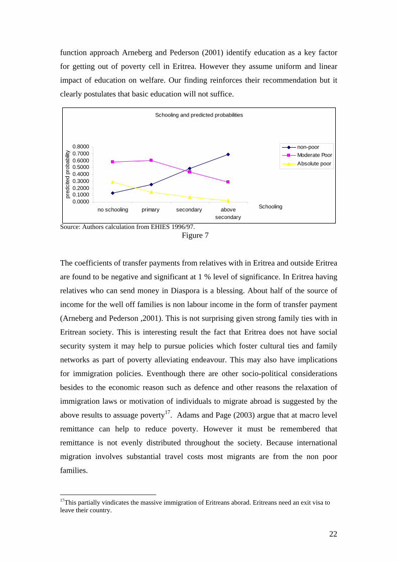
function approach Arneberg and Pederson (2001) identify education as a key factor
for getting out of poverty cell in Eritrea. However they assume uniform and linear
impact of education on welfare. Our finding reinforces their recommendation but it
clearly postulates that basic education will not suffice.
Source: Authors calculation from EHIES 1996/97.
Schooling and predicted probabilities
0.00000.10000.20000.30000.40000.50000.60000.70000.8000
no schooling primary secondary abovesecondary
Schooling
pred
cite
d pr
obab
ility
non-poorModerate PoorAbsolute poor
Figure 7
The coefficients of transfer payments from relatives with in Eritrea and outside Eritrea
are found to be negative and significant at 1 % level of significance. In Eritrea having
relatives who can send money in Diaspora is a blessing. About half of the source of
income for the well off families is non labour income in the form of transfer payment
(Arneberg and Pederson ,2001). This is not surprising given strong family ties with in
Eritrean society. This is interesting result the fact that Eritrea does not have social
security system it may help to pursue policies which foster cultural ties and family
networks as part of poverty alleviating endeavour. This may also have implications
for immigration policies. Eventhough there are other socio-political considerations
besides to the economic reason such as defence and other reasons the relaxation of
immigration laws or motivation of individuals to migrate abroad is suggested by the
above results to assuage poverty17. Adams and Page (2003) argue that at macro level
remittance can help to reduce poverty. However it must be remembered that
remittance is not evenly distributed throughout the society. Because international
migration involves substantial travel costs most migrants are from the non poor
families.
17This partially vindicates the massive immigration of Eritreans aborad. Eritreans need an exit visa to leave their country.
22

The coefficient of the number of employed persons in a household was found to be
negative and significant at less than 1% level. In addition the marginal effect shows
that it has the largest marginal effect on the probability of being poor, keeping all
other things constant. This is in line with conversional wisdom in labour economics.
Figure 8 plots the predicted probabilities of being in different poverty status and
number of employed persons in a household. It is evident from the graph that the
probability of being in absolute poverty and moderate poverty sharply decreases with
Probabilities and number of employed per household
00.20.40.60.8
1
1 2 3 4 5 6 7 8
Number of employed per household
ilitie
sob
abte
d pr
pred
ic
non poor
moderate poor
absolute poor
Source: Authors calculation from EHIES 1996/97. Figure 8
an increase in number of employed persons, keeping all other things constant. Figure
8 vividly depicts also that graph of probability of a household being non poor and
number of employed persons per household is concave. The probability of being non
poor increases at an increasing rate for the first three employed persons and thereafter
starters to increase at a decreasing rate, keeping all other things constant. These
results suggest that labour market policies could be potentially effective for tackling
poverty in Eritrea. However caution is needed before adopting such a policy
prescription. We need to ascertain if the people considered to be poor are employable
indeed. It is possible that because of the war situation and aging population most of
those who are poor and unemployed may turn out to be non employable.
Among the employment sector dummies only the coefficient of private sector
employment was found to be positive and significant at 1% level of significance.
Figure 9 reports that the probability of being poor is about 8% higher than non private
sector employee, keeping all other things same. The probability of a private sector
employee being non poor is about 9 percent lower than non private sector employee,
23

whereas the probability of being moderate poor remains almost unaltered, keeping all
other things constant. This may be partially explained by the expulsion of Non
Governmental Organizations from Eritrea which may have rendered many people
unemployed and join the poverty club. It may also reflect the presence of low paying
unskilled job categories such as housemaid and other low paying jobs which may drag
people into poverty confinement.
Predicted Probability and Private empolyment
00.10.20.30.40.50.60.7
non poor modearte poor absolutepoor Poverty status
Pred
icte
d pr
obab
ility
Non private sector employee
private sector employee
Source: Authors calculation from EHIES 1996/97. Figure 9
The coefficient for house ownership dummy was found to be negative and significant
for all categories at less than 1% level. This is in line with economic theory.
Ownership of asset is really an important indicator of poverty in most developing
countries. This indicator is of a paramount importance because it is household wealth
House ownership and predicted probabilities
00.10.20.30.40.50.60.7
non poor moderate poor absolute poverty
Poverty status
Pred
icte
d pr
obab
ility
Non house ow ners
House ow ners
Source: Authors calculation from EHIES 1996/97. Figure 10
24

which generates income flows. Figure 10 shows the effect for house ownership on the
probability of being poor and non poor. It is clear from figure 10 that house ownership
increases probability of being non poor where as it decreases the probability of being
moderate poor and absolute poor, keeping all other things constant. More specifically
it increases the probability of being non poor by more than 72 percent and decreases
probability of being moderate poor and absolute poor by 9 and 34 percent,
respectively. This can be explained by the fact that house ownership is a source of
income, property income. Secondly house ownership saves household owners from
paying huge amounts of rent which takes about two third of average income and
hence enable them spend it in non house rent expenditure. According to Arneberg and
Pederson (2001), property income is a major source of income for the households in
the top income groups in Eritrea.
The coefficient of sewage variable which is employed as a proxy for health condition
of a household is found to be negative and significant at 1% level. Access to sewage
facilities is very vital for the wellbeing of a household. Lee Gravers et al(2001)
identify that lack of sanitation facilities have negative well being effect via bad health,
reduced school attendance, gender and social exclusion and income effect( reducing
productivity ). Our results vindicate this assertion. Figure 11 reports that access to
sewage facilities decreases the probability of being moderate poor and absolute poor
by about 14 and 51, percent respectively. If we turn to the non poor category, access
to sanitary facilities increases the probability of non poor from that of with out access
to sanitary facilities by 79 percent, keeping other things constant.
Sewage and predicted probability
00.10.20.30.40.50.60.7
Non poor moderate poor absolute poor
poverty status
pred
icte
d pr
obab
ility No sew age services
Access to sew age services
Source: Authors calculation from EHIES 1996/97. Figure 11
25

The coefficient for ethnicity dummy, which takes value of one if household is
Tigrigna ethnic group other wise zero, was found to be negative and significant at 1%
level in all cases. This implies that a household from Tigrigna ethnic group has less
probability of being in poverty that non Tigrigna household, keeping all other things
predicted probabilities and ethnicity
00.10.20.30.40.50.60.7
non poor moderate poor absolute poor
poverty status
pred
icte
d pr
obob
alitie
s
Non Tigrigna
Tigrigna
Source: Authors calculation from EHIES 1996/97. Figure 12
the same. Figure 12 reports predicted probabilities for the three categories for
Tigrigna and non Tigrigna households. It is clear from the histograms in Figure 12
that being from the Tigrigna race decreases the probability of being in the moderate
poor and absolute poor, keeping al other things constant at their mean values. On the
other hand the probability of being from non poor category is higher for a Tigrigna
household than non Tigrigna household, keeping all other things the same. This may
be explained by the relative advantage of Tigrigna races access to social and capital
infrastructures. They enjoy relatively better education and other public services,
which makes their opportunity to invest in schooling significantly higher than any
other group. In addition, since the majority of the Tigrigna ethnic groups are located
in relatively big cities, their probability of wage employment is higher. There may
also be other social and other net work advantages which help them in securing job in
the large cities.
Pre-independence history of a household has also effect on a household well being.
The coefficient for the returnees from Sudan was only found to be positive and
significance at 5 % level of significance in the moderate poor category. This suggests
that the probability of being in moderate poor category is positively associated with
26

returnees being from Sudan, keeping all other things constant. The coefficient of
dummy for pre independence ex-liberation fighter was found to be negative and
significant only in the absolute poverty category at 1% level of significance. This may
imply that being a liberation ex-fighter decreases the probability of being in absolute
poverty category relative non poor category, keeping all other things constant. This
may be explained by the different affirmative actions and privileges given to ex-
liberation fighters in securing employment and acquiring party premium in the salary
scale. Fissuh(2003) finds out that there is huge party membership premium in the
determination of earnings in Eritrea. Arneber and Pederson (1999) also report that ex-
fighters get higher earnings than non ex-fighters with same qualifications which can
only be explained by political practice.
Some of the coefficients of town dummies are found to be statistically significant. The
coefficients for Akurdet, Asmara, Assab, Decemhare, and Massawa are positive and
significant at 1% level in both categories except the coefficient for Akurdet which is
not significant in the absolute poverty category. On the other hand the coefficients of
Barentu and Ghinda are negative and significant for both categories the coefficient for
Keren is found to be negative and significant at 1% level only in the absolute poverty
category. This may be explained by the remarkable difference in terms of
unemployment, weather, and level of development and population distribution
between these urban areas. The coefficient of the regional unemployment was found
to be positive and significant at 1% level of significance. It suggests a positive effect
of regional unemployment on poverty, keeping all other things constant. Hoover and
Wallace (2001) argue that robust economic growth has a positive impact on the
reduction of poverty.
CONCLUSIONS
The study uses micro level data from Eritrean Household Income and Expenditure
survey 1996-97 to examine the determinants of poverty in Eritrea. It was shown in
this paper that the DOGEV is an attractive model from class of discrete choice models
for modelling determinants of poverty across poverty categories. This paper presents
evidence of captivity of households in poverty in Eritrea. These captivities may be
27

explained by demand factors such as occupation and number of hours worked or some
social and behavioural problems.
Household size defined by adult equivalent units has significant negative effect on
the welfare status of a household. The size of the effect of household size on
poverty is not the same across the categories, though. The effect is most
pronounced in the absolute poverty category.
Age of household head was not found to be significant in linear terms in all poverty
outcomes. However the coefficient of age squared was found to be negative and
significant in the moderate poor category only. These results call further research to
understand the effect of age on poverty which has a significant repercussion to the
pension and other social security policies.
Even though education is negatively correlated with poverty, basic education will not
suffice. The coefficient of schooling is higher (absolute terms) in the absolute poor
category than in the other categories. Education is not sufficient condition to escape
from poverty. This indicates that there are other factors which affect poverty of a
household in conjunction with education. There is a need for providing
complementary factors along side with education so as to alleviate poverty.
The probability of a household being non poor is concave function of number of
employed persons per household, ceteris paribus. Besides regional unemployment rate
was found to be positively associated with poverty. These results suggest labour
market policies as potential instruments for tackling poverty in Eritrea. However
caution is needed before adopting such a policy prescription. We need to ascertain if
the people considered to be poor are employable indeed. It is possible that because of
the war situation and aging population most of those who are poor and unemployed
may turn out to be non employable.
28

Appendix
Derivation of poverty categories and definition of dummies
linepovertyregional
percapitaenditureadjustedy
exp=
The poverty variable was generated in such a way that we give more value to absolute poverty as follows:
povertyAbsolute
poverty=2 if 75.0<y
Moderate poverty:
poverty=1 if 25.175.0 ≤< y
Non poor:
poverty=0 if 25.1>y
Table 1Regional poverty lines Region poverty line with out food aid Barka/Gash Setit 225 Semhar/Sahle 275 High Land 450 Senhit 350 Keren 450 Asmara 600 Massawa 525
Source: Eritrean Poverty assessment, World Bank (1996) Notes: All poverty lines are rounded to the nearest multiple of 25 birr The above figures were adjusted by 3.5 % inflation per annum before applying to the analysis. Married= 1 if household head is married, 0 other wise.
Widowed =1 if household head is widowed, 0 other wise.
Christian=1 if household head religion is Christian, 0 other wise
Returnee from the Sudan =1 if household head returned from the Sudan after
independence, 0 otherwise
Tigrigna = 1 if household is Tigrigna race, 0 otherwise
Fighter=1 if household head is liberation ex fighter
Private sector employee= 1 if household head employed in private sector, 0 otherwise.
Government employee= 1 if household head employed in government, 0 otherwise.
Self employed= 1 if household is self employed, 0 otherwise.
Transfer from relative in Eritrea= remittance from relatives with in Eritrea
29

Transfer from relative in Diaspora= remittance from relatives in Diaspora
No formal schooling=1 if household head has no formal schooling, 0 otherwise
Elementary=1 if household head level of education is between grade 1-7, 0 otherwise
Secondary=1 if household head level of education is between grade 8-12, 0 otherwise
Pos secondary=1 if household head level of education is above grade 12, 0 otherwise
House=1 if household owns house, 0 otherwise.
Sewage=1 if household sewage and sanitation expenditure is above 0, 0 otherwise.
Adikeih=1 if town= Adikeih, 0 otherwise
Akurdet=1 if town=Akurdet, 0 otherwise
Asmara= if town=Asmara, 0 otherwise
Assab=1 if town=Assab, 0 otherwise
Barentu =1 if town=Barentu, 0 otherwise
Decemhare=1 if town=Decemhare, 0 otherwise
Ghinda =1 if town=Ghinda, 0 otherwise
Keren=1 if town=1, 0 otherwise
Massawa=1 if town=Massawa, 0 otherwise
30

Table2. Descriptive statistics
Variable Mean Std Dev Variance Minimum Maximum Poverty 1.017 0.7835 0.6138 0 2 Age of household head 4.5617 1.5801 2.4967 1.5 9.8 Age squared 2.3305 1.566 2.4524 0.225 9.604 Remittance from with in Eritrea 0.78 1.7002 2.8907 0 36.7636 Remittance from Diaspora 0.9254 3.4686 12.0311 0 87.6101 HSIZE_A 4.247 2.4255 5.8833 1 16 FIGHTER 0.1156 0.3198 0.1022 0 1 Number of employed per household 0.9596 0.7823 0.612 0 6 Regional Unemployment rate 12.6665 4.3348 18.7904 7 20 Employee in private sector 0.0983 0.2978 0.0887 0 1 Government employee 0.1484 0.3556 0.1264 0 1 Self employed 0.2241 0.4171 0.1739 0 1 HOUSE 0.496 0.5001 0.2501 0 1 SEWAGE 0.059 0.2357 0.0555 0 1 No formal schooling 0.4898 0.5 0.25 0 1 education, Grade 1-7 0.2988 0.4578 0.2096 0 1 education, Grade 8-12 0.1377 0.3446 0.1187 0 1 Above 12 grade 0.0498 0.2176 0.0474 0 1 Number of children below age of 5 0.7433 0.9046 0.8184 0 6 Number of children between age 5-15 1.193 1.3533 1.8315 0 7 Married 0.6315 0.4825 0.2328 0 1 Widowed 0.1546 0.3616 0.1308 0 1 Adikeih 0.0474 0.2126 0.0452 0 1 Akurdet 0.0647 0.2459 0.0605 0 1 Asmara 0.2214 0.4153 0.1725 0 1 Assab 0.0805 0.2722 0.0741 0 1 Barentu 0.0636 0.244 0.0596 0 1 Decemhare 0.0466 0.2108 0.0444 0 1 Ghinda 0.0523 0.2226 0.0495 0 1 Keren 0.1344 0.3412 0.1164 0 1 Massawa 0.143 0.3502 0.1226 0 1 Christian 0.3494 0.4768 0.2274 0 1 Tigrigna 0.6633 0.4727 0.2234 0 1 Returnees from the Sudan 0.0439 0.2049 0.042 0 1
Note: The following manipulations were done to ease computation by Gauss: Age/10; Age squared/100; Remittance from abroad/1000; Remittance from Diaspora/1000.
Table 3. Percentage contribution of captive probabilities on total probabilities for selected variables
Probabilities
Non poor Moderate poor Absolute poor No formal education dummy=0 0.35 0.54 0.10 0.00 12.11 9.12 No formal education dummy =1 0.13 0.58 0.29 0.00 11.34 3.30 Elementary dummy=0 0.26 0.59 0.16 0.00 -11.23 -6.00
31

Elementary dummy =1 0.25 0.60 0.15 0.00 10.95 6.53 Secondary dummy=0 0.22 0.60 0.18 0.00 10.90 5.07 Secondary dummy =1 0.49 0.44 0.07 0.00 15.03 12.94 Post secondary dummy =1 0.22 0.60 0.19 0.00 11.02 5.08 Post secondary dummy =1 0.69 0.29 0.02 0.00 22.26 47.50 Private sector employee dummy=0 0.23 0.59 0.17 0.00 11.04 5.43 Private sector employment dummy =1 0.26 0.60 0.15 0.00 10.99 6.46 Married dummy=0 0.18 0.58 0.25 0.00 11.40 3.87 Married dummy =1 0.26 0.60 0.14 0.00 10.99 6.66 Divorced house hold head dummy=1 0.21 0.59 0.20 0.00 11.20 4.74 Divorced house hold head dummy =0 0.23 0.60 0.18 0.00 11.01 5.35 Tigrigna dummy =0 0.13 0.61 0.26 0.00 10.85 3.63 Tigrigna dummy=1 0.30 0.57 0.13 0.00 11.60 7.06 Returnee from the Sudan dummy=0 0.24 0.59 0.17 0.00 11.10 5.53 Returnee from the Sudan dummy =1 0.16 0.69 0.15 0.00 9.55 6.34 Fighter dummy=0 0.23 0.60 0.18 0.00 11.03 5.31 Fighter dummy =1 0.29 0.59 0.12 0.00 11.07 7.94 Private sector employee dummy=0 0.24 0.60 0.17 0.00 10.99 5.68 Private sector employee dummy=1 0.21 0.59 0.20 0.00 11.14 5.00 Government employee dummy=0 0.24 0.59 0.16 0.00 11.05 5.74 Government employee dummy =1 0.16 0.60 0.24 0.00 10.88 3.90 House ownership dummy=0 0.18 0.62 0.21 0.00 10.64 4.52 House dummy=1 0.30 0.56 0.14 0.00 11.69 6.88 Captivity element 0.00 0.07 0.01
Note: Percentage contribution of captivity elements in bold italics under total probabilities.
32

References ADAMS, H.JR., and PAGE,J.(2003) International Migration, Remittances and Poverty in
Developing Countries ,Poverty Reduction Group, World Bank Policy Research Working Paper 3179, December 2003.
AMUEDO-DORANTES, C. (2004) “Determinants of Poverty Implications of Informal
Sector Work in Chile,” Economic Development and Cultural Change, 347-368. ARNEBER,M.W and PEDERSON, J. (1999) “Urban Households and Urban Economy in
Eritrea: Analytical, Report from the urban Eritrean Household income and expenditure survey 1996/97”, Fafo Institute for Applied Social Science, Oslo, Norway.
BARRIENTOS, A, et al(2003) “Old Age Poverty in Developing Countries: Contributions
and Dependence in Later life, World Development, 31,3:555-570. BORDERLY(1990) “The Digit model is Applicable even with out a perfectly Captive
Buyers,” Transportation research_B,24B:315-323. BOURGUIGNON, F and CHAKRAVARTY,R.S.(2003) “The measurement of
Multidimensional Poverty,” Journal of Economic Inequality, 1:25-49. CANAGARAJAH, S. and PORTNER, C.C (2003) Evolution of Poverty and Welfare in
Ghana in the 1990s: Achievements and Challenges, the World Bank, African Region Working Paper Series, No.61.
CAPPELARI and JENKINS(2002) Modelling Low Income Transitions, Institute for the
Study of Labour(IZA), discussion paper No.504. CHARLETTE-GUEARD and MESPLE-SOMPS(2001) Comprehensive System of Social
Security for South Africa, Viewpoint, South Africa Foundation, July. Johannesburg. DEATON,A.(19997)The Analysis of Household Survey micro econometric Approach to
Development Policy, The Johns Hopkins University Press, Baltimore ,Maryland. DIAMOND et al. (1990) A Multinomial Probability Model of Size Income Distribution,
Journal of Econometrics, 43:43-61. FISSUH, F.G.(2003). “Determinants of Earnings in Eritrea: a First Attempt to Estimate the
Mincerian Earnings Function’, Fiscal, Monetary and Labour policy Issues in Eritrea, Volume1 (forthcoming, 2004).
FOFACK,H.(2002) The dynamics of Poverty Determinants in Burkina Faso in the 1990s,
unpublished document. FOSTER, J. E., J. GREER , and E. THORBECKE(1984) "A Class of Decomposable Poverty
Measures." Econometrica 52.3: 761-76.
33

FRY,T.R.L. and HARRIS,M.N. (2002) The OGEV Model, Working paper 7/2002, Department of Econometrics and Business Statistics, Monash University, Australia.
GAUDRY, J.I.M.(1980) Dogit and logit models of travel mode choice in Montreal, Canadian
Journal of Economics,XII,NO.2, 268-279. GAUDRY, M., and M.DAGENAIS (1979) The Doit Model,” Transportation research-B,
13B:105-112. GEDA et al(2001) “Determinants of Poverty In Kenya: A household Level Analysis,”,
Discussion Paper, Institute of Social Studies, The Heag-the Netherlands. GLEWWE,P. (1990) Investigating the determinants of household welfare in Cote d’Ivoire,
Journal of Development Economics,35,2:307-337. GOAED,S. and M.GHAZOUANI (2001) “The determinants of urban and rural poverty in
Tunisia,” discussion paper, Laboratoire d’Econométrie Appliquée (LEA), Faculté des Sciences Economiques et de Gestion de Tunis, Tunisia.
GREENE, W.H.( 2003) Econometric Analysis, 5th Ed., Prince Hall ,USA.
HARRIS, et al.(2002) Who are the self-employed? A New Approach, Working Paper,
11/2003, Department of Econometrics and Business Statistics, Monash University, Australia.
JOLLIFE, D. and DATT,G.(1999) Determinants of Poverty in Egypt:1997,FCND Discussion
paper no.74, Food consumption and Nutrition division, IFPRI, Washington, D.C. JOLLIFE,D.(2003) On the relative well-being of the non metropolitan Poor: An examination
of Alternate Definitions of Poverty During the 1990s, Southern Economic Journal,70,2: 295-311.
KABUBUO-MARIARA,J.(2002) Herds response to Acute land Pressure and Determinants
of Poverty under Changing Property Rights: Some Insights from Kenya, EEE Working paper series , N0.2.
KOPPELMAN ands SETHI (2000) Closed Form Discrete Choice Models, Department of
Civil Engineering, lecture note, North Western University, USA. LADERCHI, R.C. et al (2003) Does it Matter that we do not Agree on the Definition of
Poverty? A Comparison of Four Approaches, Oxford Development studies, 31, 3:243-274.
LANJOUW,P and M.RAVALLION (1995) "Poverty and Household Size", The Economic Journal, vol. 105, pp.1415-1434.
LEE TRAVERS et al (2001) Water, Sanitation and Poverty, Draft for Comments. April, 2001
available on line at [accessed on 14th of May, 2004:3:00pm] http://www.worldbank.org/poverty/strategies/chapters/water/wat0427.pdf
34

MADDALA, GS. 1983. Limited-Dependent and Qualitative Variables in Econometrics, Cambridge: Cambridge University Press.
MCKAY,A. and COLOUBE,H. (1996Modelling Determinants of Poverty in Mauritania, World Development,24,6:1015-1031.
MESPLE-SOMPS, S. and GUENARD, C.M.G.(?) What happened to the urban population in
Cote d’Ivoire since the 1980s? An analysis of monetary and deprivation over 15 years of household data, DIAL, Research Unit CIPRE of Institu de Recherche pour le Development, Paris, France.
MULLER, C.(1999) Censored Quantile Regressions of Poverty in Rwanda, CREDIT
research papers,no.99/11. Okwi,P.O.(1999) Poverty In Uganda, Economic Policy Research Centre working papers,
Makerere University, Uganda. RAVALLION, M.(1996)Issues in Measuring and Modelling Poverty, The Economic
Journal,106,1328-1343. ROUBAND, F. and RAZAFINDRAKOTO, M.(2003) The Multiple Facets of Poverty: the
case of urban Africa, provisional version, DIAL, Paris. ROUBAUD, F. and RAZAFINDRAKOTO, M.(2003) “The multiple facet of poverty: the
case of Urban Africa, Provisional version SCHOUMAKER, B.(2004) Poverty and Fertility in Sub-Saharan Africa: Evidence from 25
countries, draft paper presented at the Population Association of America Meeting, Boston, April 1-3.
SMALL, A.K.(1987)A discrete Choice Model for Ordered Alternatives,
Econometrica,55,2:409-424. The International Food Policy Research Institute (2001) The determinants of Poverty in
Malawi: An analysis of the Malawi Integrated Household Survey,1997-98, in collaboration with National Economics council, Lilongwe, and The National Statistical Office, Zomba, Malawi, Washington ,DC, USA.
WALLACE, G.L. and HOOVER, G.A.(2003) Examining the Relationship between the
Poverty Rate and Economic Conditions: A Comparison of the 1980s and 1990s,Working Paper no.03-10-01, University of Wisconsin, Madison, USA.
WOOLDRIDGE,J.M (2002) Econometric analysis of cross section and panel data, 2nd ed.,
The MIT press, London, England. World Bank (1996) “Eritrea poverty Assessment,” Report No.15595-ER,The World Bank,
Washington, D.C, USA.
35