Embed Size (px)
Citation preview

0
No. 54
February 2013
Teguh Dartanto and Shigeru Otsubo
Analyses of Multifaceted Poverty and Poverty Dynamics in Indonesia
Measurements and Determinants of Multifaceted Poverty: Absolute, Relative, and Subjective Poverty in Indonesia

Use and dissemination of this working paper is encouraged; however, the JICA
Research Institute requests due acknowledgement and a copy of any publication for
which this working paper has provided input. The views expressed in this paper are
those of the author(s) and do not necessarily represent the official positions of either the
JICA Research Institute or JICA.
JICA Research Institute
10-5 Ichigaya Honmura-cho
Shinjuku-ku
Tokyo 162-8433, JAPAN
TEL: +81-3-3269-3374
FAX: +81-3-3269-2054
Copyright ©2013 Japan International Cooperation Agency Research Institute
All rights reserved.

1
Measurements and Determinants of Multifaceted Poverty:
Absolute, Relative, and Subjective Poverty in Indonesia
Teguh Dartanto* and Shigeru Otsubo†
Abstract
The notion of ‘poverty’ is diversified and dynamic. It varies across countries with different
socio-economic norms. It may also change over time even in the same society, with different
stages of social and economic development. A country may be struggling with absolute poverty
at the early stages of development, while it may well be more concerned with relative and/or
subjective poverty as its average per-capita income increases. This article intends to conduct an
exploration of multiple poverty measures by looking into the absolute, relative and subjective
poverty incidence in Indonesia. Using the 2005 National Socio-Economic Survey (Susenas), we
observed that there was a roughly 28 percentage-point difference in the poverty headcount ratios
computed by applying absolute (14.47%) and subjective (42.03%) poverty. There were virtually
no correlations among the poverty rankings in the provinces of Indonesia obtained by five
poverty metrics. Results of logit model and ordered logit model estimations of the possible
determinants of poverty indicate that the main determinants of poverty are educational
attainment, number of household members, physical assets (land and house ownership),
existence of migrant workers (possible remittances), negative shocks of layoffs and/or health
problems, development of public services, and the availability of road infrastructure. A higher
educational attainment increases the probability of never being poor in any of the five poverty
metrics by almost 11 percentage points. This study also confirmed that households having less
than society’s averages in terms of the physical asset of land and consumption of durable goods
and fashion tended to subjectively asses themselves as poor. The study suggests that any poverty
alleviation programs should consider relative impacts among beneficiaries and non-beneficiaries
within each locality and across provinces.
Keywords: Absolute Poverty, Relative Poverty, Subjective Poverty, Subjective Well-Being,
Multidimensional Poverty Analysis, Indonesia
* Research Associate, Japan International Cooperation Agency Research Institute ([email protected]) † Professor, Graduate School of International Development, Nagoya University, and Visiting Fellow, Japan International Cooperation Agency Research Institute This research was conducted as a research project at the Japan International Cooperation Agency Research Institute. The study is also partly funded by the Japan Society for the Promotion of Science (JSPS) Research Funds (Kiban A-22252005 and Challenging Exploratory Research 23653066). The views expressed in this paper are those of the authors and do not necessarily represent the official positions of either the JICA Research Institute or JICA. Authors would also like to thank the two anonymous referees for their constructive and valuable comments and suggestions.

2
1. Introduction
Problems associated with the definitions and measurements of ‘poverty’ have been debated
over decades. Poverty is a multifaceted phenomenon and different societies have different
perceptions of ‘poverty.’ Although he did not directly refer to the notion of ‘poverty,’ Smith
(1776) (Sen 1983) noted that the Greeks and Romans lived very comfortably though they had
no linen; but in the present time, through the greater part of Europe, an average day laborer
would be ashamed to appear in public without a linen shirt. This means that although a linen
shirt had become the norm for European society in the 1770s, it was not the case in ancient
Greek or Roman societies. The perception of the ‘necessaries,’ and therefore ‘poverty,’ is
diversified and dynamic. It varies across countries with different socio-economic norms. It
may also change over time even in the same society, with different states of development.
Most researchers agree that poverty can be conceptualized in the forms of deprivation
suffered by the population. Various notions of poverty can then be classified as: 1) absolute
poverty, 2) relative poverty, and 3) subjective poverty. Absolute poverty means that people
have less than the objectively defined thresholds such as the minimum food-calorie intake and
basic needs. Those with income (expenditure) below a certain money metric of basic needs are
then classified as poor. Relative poverty refers to the definition that poverty is having less than
others in the same society (Hagenaars and de Vos 1988). Subjective poverty means that
individuals appraise their poverty status by themselves, subjectively. People would simply be
categorized as poor when they consider themselves so (Niemietz 2011).
Applying different notions/metrics of poverty might produce different analytical
results that, in turn, call for a different set of policy interventions. For example, while absolute
poverty may be reduced by economic growth, relative poverty can only be mitigated when
income inequality decreases (Hegenaars and Van Praag 1985). While absolute poverty may
disappear as countries become richer, the relative deprivation and subjective poverty may

3
persist. Thus, while most developing countries are still concerned with absolute poverty, many
developed countries, particularly OECD economies, have already shifted their focus to relative
and subjective poverty.
In the past three decades, except for the periods of crises, socio-economic conditions in
Indonesia have been improving rapidly. During this period, per-capita GDP in Indonesia
increased three-fold. The World Bank reported that the per-capita GDP (PPP, 2005 US$) of
Indonesia had jumped from $1,323 (1983) to $4,094 (2011).1 This substantial increase in
income has been accompanied by improvements in social indicators such as a massive
decrease in absolute poverty incidence from 28.6% (1980) to 13.3% (2010) in headcount ratios,
and a significant increase in the gross enrollment rate for tertiary education from 4% (1981) to
23% (2010).2 These rapid changes in income and education attainments, coupled with ongoing
technological innovations, have influenced society’s perception of poverty. For example, in
1998, the Central Statistical Agency of Indonesia (henceforth BPS) changed the method of
calculating the poverty line by adopting the adjustments for the quality of non-food items.3
The absolute poverty measurements might be appropriate in the past and current
context in Indonesia, but might not be suitable for the future. In the early stage of development,
where there were high levels of hunger, society’s and government’s perception of poverty was
dominated by absolutist concerns. However, when almost all members of society can easily
afford basic needs, society’s focus shifted from absolute deprivation to relative deprivation.4
1. http://data.worldbank.org/indicator/NY.GDP.PCAP.PP.KD. 2. http://www.bps.go.id/tab_sub/view.php?kat=1&tabel=1&daftar=1&id_subyek=23¬ab=1 3. Since 1998, a change in the method of calculating the poverty line was adopted by improving the quality of non-food items, including: the cost of education (originally based on the cost of elementary education, the increase to cover the costs of junior high school education), the cost of health care (initially based on standard costs at a primary Health Center, then increased to include the costs of services of a general practitioner), and the transport costs (initially only costs of transport within a city were estimated, then transport costs were increased to also provide for inter-city transportation costs in accordance with the increased mobility of the population). As a result, the poverty line increased and the population below the poverty line also increased. 4. Corazzini, Esposito and Majorano (2011) observed undergraduate students from eight countries(Bolivia, Brazil, Italy, Kenya, Laos, Sweden, Switzerland and the UK) and concluded that students coming from richer countries tended to see poverty from a more relative perspective as compared to their colleagues from lower-income countries.

4
In a diverse society like Indonesia where a great deal of regional disparities exist, the
perception of poverty among those living in Jakarta, the most developed province with
per-capita income at around $4,500/year (2010), might be totally different from that of those
living in East Nusa Tenggara (NTT), the poorest province with per-capita income of less than
$300/year (2010).5 A person in NTT might perceive poverty as the deprivation of basic needs
while a person in Jakarta might perceive poverty as relative deprivation. Thus, the government
of Indonesia should not only update the absolute measures but also compile relative or
subjective measures of poverty. While an absolute measurement helps us to identify those
people who are not able to attain a minimum standard of living, a relative measurement assists
us in identifying those whose standard of living is low compared to the average level of the
society in which they live. The subjective measurements of poverty help to evaluate the
satisfaction/happiness/well-being of members of society, while promoting discussions about
the goals of development. Figure 1 shows one proto-typical framework of the relationship
between the stages of development, social issues, poverty measurements, and policy
interventions.6
5. The per-capita income refers to GDP per-capita calculated based on the 2000 constant price. http://www.bps.go.id/tab_sub/view.php?kat=2&tabel=1&daftar=1&id_subyek=52¬ab=2. 6. Social issues and policy interventions often continue into the later stages of development. For example, the issues associated with ‘social exclusion’ persist even among the most advanced countries.

5
Figure 1. Stages of development, social issues, poverty measurements, and policy interventions
Source: Authors
Absolute poverty analyses that compare the levels of income or expenditure with the
given thresholds have dominated poverty literature in Indonesia (Islam and Khan 1986; Bidani
and Ravallion 1993; Booth 2000; Balisacan, Pernia, and Asra 2002; Fields et al. 2003;
Suryahadi, Suryadarma, and Sumarto 2009; Dartanto and Nurkholis forthcoming). Given the
dynamism of society’s perception of ‘poverty’ and rapid changes in the socio-economic
situation in Indonesia, the current study of multiple poverty indicators should be a valuable
addition to the existing stock of poverty literature. It is the first comprehensive study in
Indonesia that looks into not only objective poverty (absolute and relative poverty), but also
subjective poverty measurement. The subjective poverty measurements can be used to evaluate
whether or not the current official absolute poverty line properly represents society’s
6
perception of poverty. There may be significant differences between objectively and
subjectively measured poverty in Indonesia.
Comparing the determinants of poverty across different poverty measures allows us a
better understanding of the roles and robustness of various determinants of poverty. It also
helps us to detect the key determinants that policy initiatives should focus on. It should also
widen the perspective of Indonesian policy makers in proposing poverty alleviation policies.
Existence of absolute and/or relative poverty would call for a different set of strategies to cope
with. In a region where the problem of poverty is characterized by objective/absolute poorness,
then the appropriate strategy would be promoting economic growth through providing basic
physical and human capital infrastructure. If the existing problems in other regions are related
to relative poverty, then the proper strategy may well include policies that promote asset
redistribution. Alesina and Perotti (1996) mentioned that income inequality and life
dissatisfaction (well-being) are closely related to political instability—an important agenda for
development in Indonesia where national unity has been a priority issue.
This article, therefore, intends to conduct comparative studies of multiple poverty
measures by looking into objective/absolute, relative and subjective poverty incidence in
Indonesia. This paper aims at addressing the following three main questions: 1) How different
are the poverty outcomes if five different metrics of poverty are used? 2) What are the key
determinants of absolute, relative and subjective poverty? and 3) Are the socio-economic
indicators of the reference group (neighbors) correlated with households’ assessment of their
subjective poverty?
The next section of this article presents a literature review on poverty definitions and
past research on absolute, relative, and subjective poverty metrics. Section three describes the
current research methodology. Section four introduces the national and regional poverty profile
of Indonesia. The fifth and the main analytical section of the paper will introduce the results of
logit and ordered logit model analyses of the determinants of absolute, relative, and subjective
7
poverty. The concluding section of the paper will summarize the main findings and discuss
their policy implications.
2. Literature review
2.1 Defining poverty
Although the researchers in the field of poverty analyses have employed a wide variety of
definitions, all poverty definitions can fit into one of the following categories: absolute poverty,
relative poverty, and subjective poverty (Hagenaars and de Vos 1988). In the absolute poverty
concept, poverty means that one is having less than the objectively-defined absolute minimum.
The Basic needs approach defines this absolute minimum in terms of ‘basic needs’ such as
food, clothing, and housing. Second, in the relative poverty concept, poverty means that one is
having less than others have in the same society. Relative deprivation with respect to various
commodities defines households as poor when they are lacking certain commodities that are
common in the society they belong to (Townsend 1979). Third, in the subjective poverty
concept, poverty means that one is feeling that (s)he does not have enough to get along. In the
subjective minimum income definition, one is said to be poor if one’s actual income level is less
than the amount (s)he considers to be ‘just sufficient’ (Goedhart et al. 1977).
Perhaps, the earliest systematic studies on poverty were pioneered by Benjamin
Seebohm Rowntree in the city of York, and by Charles Booth in London at the end of the 19th
century. Rowntree defined poverty as families whose total income is insufficient to obtain the
minimum necessities for the maintenance of merely physical efficiency (1901, 86). Rowntree
called poverty falling under this category as ‘primary’ poverty. Rowntree’s definition of
poverty was apparently an absolute/objective poverty concept. Townsend (1954) criticized
Rowntree’s framework, stating that it ignored social needs, asserting that Rowntree’s

8
framework should be extended to include not only physical efficiency but also social
participation costs.
Townsend (1962) argued that there were no purely physical needs. Needs are almost
completely a social concept, and society itself is continuously changing. While defending the
‘absolute core’ in the idea of poverty, Sen (1979) stated that the notion of ‘minimum needs’
must be relative rather than absolute. Poverty has to be judged in comparison with the
experience of others in society. Sen (1983) asserted that the relativist approach sees deprivation
in terms of a person or a household being able to achieve less than what others in that society
do, and this relativity is not to be confused with variation over time. Most OECD countries use
a relative poverty line and set it at typically 40-60% of mean or median income (e.g., Fouarge
and Layte 2005; Eurostat 2005; OECD 2008). The argument of using a constant proportion of
the mean relates to the costs of ‘social inclusion’, the cost assuring a person can maintain
personal dignity and participate in customary social activities.7 In the case of developing
countries, Ravallion and Chen (2011) found that, in 2005, one half of the population of the
developing world lived in relative poverty, half of whom were absolutely poor. The total
number of relatively poor rose during the period 1981–2005, despite falling numbers of
absolutely poor.
In contrast to the absolute and relative poverty measures, which are mostly constructed
from the objective data of expenditure and/or income, subjective poverty is based on
psychological perceptions of individuals. Niemietz (2011) summarized the two definitions of
subjective poverty: the first one consists of an individual assessment of their poverty status.
People are simply classified as poor when they consider themselves so. In this version of the
subjective poverty concept, there is no setting of the ‘poverty line’. The second one involves a
majoritarian or democratic approach to setting the poverty line. People can be asked directly
what they consider to be the necessary minimum income to maintain a minimum decent
7. Personal dignity is also often advocated in the area of absolute poverty.

9
standard of living in their society. The average responses obtained from surveys utilizing the
minimum income question (MIQ), the income evaluation question (IEQ), the consumption
adequacy question (CAQ), and the economic ladder question (ELQ) then become the
foundation of the poverty line. Contributions to the majoritarian poverty line analyses include
Goedhart et al. (1977), Danziger et al. (1984), Kapteyn, Kooreman and Willemse (1988), and
Pradhan and Ravallion (2000). However, Deaton and Zaidi (2002) indicated that MIQ
methodology might not be applicable to most developing countries where income is not a
well-defined concept, particularly in rural areas.
Two prominent examples of subjective well-being research are the General Social
Surveys (Davis, Smith and Marsden 2001) and the World Values Survey (Inglehart et al. 2000).
The General Social Surveys has a single-item question on a three-point scale. This survey asks
the question: “Taken all together, how would you say things are these days - would you say
that you are very happy, pretty happy, or not too happy?” The World Value Survey assesses life
satisfaction on a scale from one (dissatisfied) to ten (satisfied). This survey asks the question:
“All things considered, how satisfied are you with your life as a whole these days?” Frey and
Stutzer (2002) summarized that people evaluate their level of subjective well-being with regard
to circumstances and in comparison to other persons, past experience and expectations of the
future.
The General Social Survey and the World Values Survey ask directly on subjective
well-being/life satisfaction in one question. However, life satisfaction can also be evaluated by
a two-layer model (Van Praag and Ferrer-i-Carbonell 2008). In this case, the first layer asks
households the question: “How satisfied are you today with the following areas of your life?”
with answers, on a scale from one to ten, for areas such as income satisfaction, health
satisfaction, job satisfaction, environment satisfaction and so on. The second layer then
combines all components of the evaluation of households as overall life satisfaction.

10
2.2 Determinants of absolute, relative and subjective poverty
Many past studies have found that the key determinants of absolute poverty8 are human capital,
demographic factors, geographical location, physical assets and occupational status. Hassan
and Babu (1991) found that productive assets other than land, smaller-sized families, and
higher non-farming-related earnings are the determinants of food (calorie) poverty in rural
Sudan. Studies by Rodriguez and Smith (1994) in Costa Rica, Adam and Jane (1995) in
Pakistan, Grootaert (1997) in Cote d'lvoire, Anyanwu (2005) in rural Nigeria, Mukherjee and
Benson (2003) in Malawi, de Silva (2008) in Sri Lanka, Dartanto and Nurkholis (forthcoming)
in Indonesia have clearly shown that an increase in human capital indicated by educational
attainment decreases the probability of being poor and improves the ability of a household to
respond to transitory shocks. With regard to the changes in demographic factors, a positive link
between an increased household size and poverty has been confirmed by Mukherjee and
Benson (2003) in Malawi, Anyanwu (2005) in Nigeria, Mok, Gan and Sanyal (2007) in
Malaysia, and de Silva (2008) in Sri Lanka.
de Silva (2008) confirmed in Sri Lanka that poverty is commonly found in rural areas.
A lack of physical assets is another important factor often associated with poverty (Adam and
Jane 1995; Grootaert 1997; de Janvry and Sadoulet 2000; Mukherjee and Benson 2003). Lastly,
occupation status is frequently found as one of the important factors determining the household
poverty status. Rodriguez and Smith (1994), Fields et al. (2003), and de Silva (2008) found
that households with the head working as a waged employee can escape poverty. In the case of
Indonesia, Fields et al. (2003) and Dartanto and Nurkholis (forthcoming) confirmed that the
important factors of poverty dynamics are educational attainment, number of household
8. Some researchers called absolute poverty as objective poverty since this poverty is calculated based on the objectively defined threshold of minimum consumption. In this current analysis, the five poverty metrics for calorie, expenditure, relative, SWB, and subjective poverty definitions can be divided into objective measures (calorie, expenditure, and relative poverty measurements) and subjective measures (SWB and subjective poverty measurements).

11
members, physical assets, employment status, health shocks, access to electricity, and changes
in the household size, sectors in which they work, and the availability of microcredit programs.
Compared to the abundant research on absolute poverty, there has been little analysis
on the determinants of either relative or subjective poverty, particularly in developing countries.
Kenworthy (1999), assessing 15 affluent industrialized nations over the period of 1960–91,
strongly supported the conventional view that social-welfare programs reduce both absolute
and relative poverty. Moller et al. (2003), using the panel data of 14 OECD countries between
1970 and 1997, found that relative poverty is mainly a function of industrial employment,
unemployment, wage coordination and welfare policies. Herrera, Razafindrakoto and Roubaud
(2006) modeled the determinants of subjective well-being in Peru and Madagascar by
including several explanatory variables such as household demographic characteristics,
socio-economic characteristics, social and political participation, shock and vulnerability, and
social comparisons. They found that in Madagascar and Peru income inequality had a negative
effect on the individual subjective evaluation of poverty.
Luttmer (2005) estimated the determinants of well-being as a function of own income
and control variables such as religion, age and other socio-economic indicators and found that
higher earnings of neighbors were associated with lower levels of self-reported happiness.
Kingdon and Knight (2006), investigating subjective well-being (SWB) poverty in South
Africa, found that the determinants of SWB poverty were age, household unemployment rate,
health problems, house ownership, ethnicity, and availability of community roads. Ladiyanto et
al. (2010) found that happiness in Indonesia depends on age, education, health, assets,
marriage, and expenditure. Frey and Stutzer (2002) reported that subjective well-being is a
valid and empirically adequate measure for human well-being, and asserted that it can be
modeled in a microeconometric happiness function that can be estimated by ordered probit or
logit models.

12
3. Research methodology
3.1 Operationalizing poverty definitions
This article classifies poverty experienced by Indonesian households using five poverty
indicators: i) calorie intake poverty, ii) expenditure poverty, iii) relative poverty, iv) subjective
well-being (SWB) poverty and v) subjective poverty. While i) and ii) reflect an ‘absolute’
notion of poverty, iii) reflects a ‘relative’ notion of poverty. Metrics i), ii), and iii) can be
grouped as ‘objective’ measurements of poverty against the ‘subjective’ measurements of iv)
and v).9 This study uses the 2005 National Socio-Economic Survey (Susenas) collected by the
Central Statistical Agency of Indonesia to quantify poverty in all five measures, and to analyze
determinants of these multifaceted poverty metrics. The Susenas survey covering all provinces
in Indonesia except Aceh consists of two main datasets: Core and Module. The Susenas 2005
Core recorded the detailed characteristics of 278,352 households representing the 59,321,125
households in Indonesia and covering various geographic regions of the country. The 2005
Susenas Module collected additional pieces of information on a subset of the Core households
(68,288 households). The Susenas Module recorded detailed sets of information for food and
non-food consumption as well as income of the sample households. After merging the Susenas
Core and Module and omitting the missing and outlier data, 62,625 households are included in
the current analyses.
A person suffers from absolute deprivation if (s)he cannot enjoy society’s minimum
standard of living. If one accepts a definition of a minimum standard of living as consumption
at a certain level known as the poverty line, then the poverty measurement is straightforward:
those with consumption expenditures below this line are considered ‘poor’ and the rest are
‘non-poor’.
9. Relative poverty measurements can also be defined as subjective indicators.

13
If we use the calorie poverty line, then those with daily food consumption worth less
than 2,100 Calories (≅ kilocalories) are classified as poor (Ravallion 1994). The 2005 Susenas
Module recorded 229 food commodities consumed by households. Using the calorie contents
of each food, BPS calculated the calorie intake for each household. If we use the expenditure
poverty line, then those with monthly expenditure for both foods and non-foods less than the
2005 BPS poverty line are classified as poor.10 The BPS poverty line varies across provinces
and between rural and urban areas.11 This is due to the differences in food and non-food prices
and in consumption patterns. The calculation of poverty using the expenditure approach is the
official measurement of poverty in Indonesia.
When the relative poverty concept is applied, those with monthly income less than 50
percent of the average provincial income are categorized as poor.12 Sen (1979) said that the
income of a person can be seen to be not simply a rough aid to predicting a person's actual
consumption, but also as capturing a person's ability to meet his minimum needs. The income
in the 2005 Susenas survey covered four components: 1) monthly wages (salaries) and
non-wage (salary) reward, 2) yearly net-income from agriculture and non-agriculture business,
3) yearly incomes from rent, shares and interest, and 4) yearly transfers. Like the BPS poverty
line, this relative poverty line also differs across provinces and between rural and urban areas.
10. The Central Statistical Agency of Indonesia’s use of 2,100 Calories/capita/day resulted from 52 commodities designed for calculating the food poverty line. To calculate the expenditure poverty line, non-food expenditures such as on health, education, transportation, etc., should be added. 11. In 2005, the average monthly money metric of the national poverty line was IDR 117,259 ($11.7) in rural areas and IDR 150,799 ($15) in urban areas. 12. This study used income instead of expenditures for the calculation of the relative poverty line in order for us to obtain a consistent set of poverty indicators. Atkinson and Bourguignon (2001) postulated two key capabilities in the poverty measurements: physical survival and social inclusion. Therefore, the relative poverty line should not be set lower than the absolute poverty line (a physical survival need). However, if we set the poverty line at the level half (50%) of the mean (median) expenditures, this will make the relative poverty line at a level lower than the absolute poverty line. Therefore, the relative poverty incidence particularly in rural areas will be lower than the absolute poverty incidence. For example, using the 50% mean of expenditure as the relative poverty line will result in a poverty incidence of 19.64% (Urban) and 9.52% (rural), while using the 50% median of expenditure as the relative poverty line will result in a poverty incidence of 14.33% (urban) and 10.17% (rural). Both results are lower than the absolute poverty incidence.

14
For subjective well-being poverty, this study adopts the weakly defined SWB poverty
concept in accordance with the ways the relevant questions were raised in the survey for the
2005 Susenas.13 Most of the survey questions related to the SWB poverty are similar to those
of World Values Survey and General Social Survey. However, the 2005 Susenas evaluated the
subjective perception of household consumption by the following questions:14
1) (Food Consumption) Compared to that of last year, what is the current level of
food consumption? 1) significantly decreased; 2) slightly decreased; 3) same; 4)
slightly increased; 5) significantly increased
2) (Non-food Consumption) Compared to that of last year, what is the current level of
food consumption? 1) significantly decreased; 2) slightly decreased; 3) same; 4)
slightly increased; 5) significantly increased
We then assigned numerical scores from 1 to 5 to each question. Adding up the scores for the
two sub-questions, the total score ranges from 1 to 10. Poor is defined as those with a total
score of 5 or less.15
The subjective poverty definition used in this study follows that of Niemietz’s category
of an individual assessment instead of a majoritarian (democratic) poverty line. Those who
reported themselves as poor are categorized as poor. In the 2005 Susenas, respondents are
asked the following question: “In your opinion, do you think you are poor?” 1) Yes; 2) No. If
respondents reported yes, then they are categorized as (subjectively) poor in this subjective
poverty concept. 13. Households' evaluation on consumption of both foods and non-food items in Susenas is only one part of life satisfaction. Thus, the SWB measurement obtained from this Susenas may be called ‘weakly defined’ SWB or ‘pseudo’ SWB. The current study then followed the two-layer approach of Van Praag and Ferrer-i-Carbonell (2008) by combining the scores of households' evaluation on both foods and non-food items. 14. Addressing questions in changes over a certain periods, not in levels, is also widely seen among surveys of subjective well-being. For example, in their study on Madagascar and Peru, Herrera, Razafindrakoto and Roubaud (2006) used the following question for the households' subjective assessment of the evolution of living standards. During the last year, living standards have: increased, stagnated, or fallen. 15. If a household experiences significant increase in either food or non-food consumption but at the same time experiences significant decrease in the other consumption category, then that household is still categorized as non-poor.

15
3.2 Two models for the determinants of poverty
The current study uses two econometric models—logit and ordered logit models—in order to
examine the determinants of poverty outcomes under the aforementioned five poverty concepts.
The logit model is applied to observe the determinants of each poverty category. That is, why
some households are categorized as poor in a designated poverty category while others are
categorized as non-poor (Eq.1). The ordered logit model is applied in order to examine the
relative effects of different household characteristics on their poverty outcomes. That is, why
some households only experience poverty in one poverty indicator while others experience
poverty in two to all five poverty categories (Eq.2). The description and descriptive statistics of
each of the explanatory variables included in these models are summarized in Appendix 1 and
2. Mean and standard deviation of each explanatory variable are also presented in Appendix 3
for the poor identified by each one of the aforementioned five poverty concepts. Cross
correlations among five poverty indicators and explanatory variables are presented in
Appendix 4. Independent variables are selected taking into account data availability in the
2005 Susenas and the results of the previous studies, such as Hassan and Babu (1991), Adam
and Jane (1995), Grootaert (1997), Frey and Stutzer (2002), Mukherjee and Benson (2003),
Fields et al. (2003), Bigsten et al. (2003), Kedir and McKay (2005), Anyanwu (2005), Luttmer
(2005), Kingdon and Knight (2006), de Silva (2008), and Dartanto and Nurkholis
(forthcoming).
The logit and ordered logit models are as follows:
[1]
[2]
where,
• is a household poverty category for each of five poverty indicators: 1 = poor,
0= non-poor;
iiiiiiLMi eRELREGCHARShockGovSECOHHCy +++++= γϕφχβ
iiiiiiOLMi eRELREGCHARShockGovSECOHHCy +++++= γϕφχβ
LMiy

16
• is a household poverty experience: 0 = non-poor in all of the five poverty
measurements; 1 = poor in only one poverty measurement; 2 = poor in two poverty
measurements; 3 = poor in three poverty measurements; 4 = poor in four poverty
measurements; 5 = poor in all of the five poverty measurements;
• is a vector of family characteristics including marital status, age, education
attainment, number of household members, number of children under 5 years of age,
and a locational dummy (1=urban or 0=rural);
• is a vector of socio-economic characteristics including employment status,
land ownership (in hectares), size of house (in square meters), a dummy for households
with some members working as overseas migrant workers, and a ratio of self-food
production over total food consumption;
• = a vector of shocks, coping strategies, and policy assistances received;
Negative shocks include layoffs and health problems. Positive shocks are an
improvement in public facilities in the surrounding area. This vector also includes
interaction variables (cross-terms) between layoffs and public provision of cheap rice
(RASKIN), between health shocks and public provision of health insurance targeted to
the poor (ASKESKIN). This vector also includes availability of household savings to
cope with the shocks.
• is a vector of regional characteristics including agricultural productivity
for food crops, human development index, proportion of paved roads, and proportion of
sanitation availability in each region where household i resides;
• is a vector of household’s conditions relative to the averages of that society;
This vector includes relative size of land and housing ownership, relative development
of public facilities, relative educational attainment, relative consumption of durable
goods and fashion items, and relative access to telephone and Internet.
OLMiy
iHHC
iSECO
iShockGov
iREGCHAR
iREL

17
• is an error term; and
• i is the household identifier ( i=1,…, 62,625).
Eq. 1 is a binary response model with two outcomes y={0,1} while Eq. 2 is an ordered
response model with six outcomes y={0,1,…,5}. An ordered probit model (probit model) for y
(conditional on a vector of explanatory variables x) can be derived from a latent variable model.
Assume that a latent variable y* is determined by,
Normal (0,1) [3]
where is a k x 1 coefficient vector, and for reasons to be seen, vector x does not contain a
constant (for the detailed explanation of the ordered response model, see Wooldridge (2010)).
The parameters of this model can be estimated by using the maximum likelihood
estimation. The signs of estimated coefficients from the ordered probit/logit models have
exactly the same meaning as those obtained from the ordinary-least-square (OLS) estimations.
A negative sign implies that the choice probabilities shift to lower categories when the
independent variable increases. The magnitudes of the estimated coefficients, however, cannot
be interpreted directly as in the case of OLS estimations. In most cases, we are interested in the
response probabilities or partial effects ( )xjyP = of the ordered probit/logit models (for the
detailed explanation of the response probabilities, see Wooldridge (2010).
4. Multiple poverty indicators and regional characteristics in Indonesia
Table 1 presents a cross tabulation of 62,625 Indonesia households extracted from this 2005
Susenas, being classified as poor or non-poor in each one of the five operationalized poverty
definitions. While 85.53% of households are categorized as absolute (expenditure) non-poor
(i.e., 14.47% as poor), only 57.97% of households are reported subjective non-poor (i.e.,
42.03% as poor). While 37.15% (19,900/53,566) of households that are absolute (expenditure)
non-poor reported themselves as subjectively poor, 29.12% (2,638/9,059) of the absolute
e
,* exy += β xe
β

18
(expenditure) poor reported as non-poor in their subjective judgment category. This evidence
indicates that some households that are non-poor in an objective measurement may still feel
poor subjectively. In the same token, other households that are poor in an objective metric
could still perceive themselves non-poor in a subjective metric.
Table 2 presents computed poverty indicators using the aforementioned five poverty
definitions for provinces of Indonesia together with other key regional characteristics. In
Indonesia, it is generally said that there are two types of regional segregation, Java and Bali
versus outside Java and Bali, and Western Indonesia versus Eastern Indonesia. Western
Indonesia comprises of Sumatra, Java, Bali and Kalimantan, while Eastern Indonesia consists
of Sulawesi, Nusa Tenggara, Maluku and Papua. Highly populated Java and Bali areas are
significantly more developed than other islands in terms of economic activities and
infrastructure. While manufacturing activities and service sectors dominate the economy of
Java and Bali, agriculture and mining activities dominate the economy outside Java and Bali.
According to the BPS, in 2005 (survey year), the Java-Bali economy contributed 61.2% of
Indonesian Gross Domestic Product. The population in these areas also amounts to 58.8% of
Indonesia’s total population. Table 2 confirms that Java-Bali provinces generally have better
road infrastructure, higher agricultural productivity, and lower criminal risk as compared to
other provinces.
This regional segregation between Java-Bali and outside Java-Bali provinces may well
influence the regional patterns of poverty incidence. Table 2 shows that, in fact, the poverty
incidence across provinces varies in all poverty measures. The national poverty incidences in
2005 were 3.57% (calorie), 17.44% (expenditure), 30.83% (relative), 33.73% (SWB) and
38.94% (subjective). There were 21.5 percentage-point differences in the poverty outcome
between absolute and subjective poverty.16
16. Poverty outcomes at the national level reported in Table 2 differ from those reported in Table 1. In Table 2, national averages are obtained by weighting regional indicators with regional populations, whereas Table 1 reports the unweighted national statistics.

19
Table 1. Cross tabulation between each poverty indicator
Note: For each cell, the first row contains the number of households in that category. The numbers in the second row show percentage share in total sample households. Source: Authors’ calculation.
The highest level of absolute poverty both in calorie and expenditure measurements is
found in Papua (16.89% and 43.95%, respectively) while the lowest calorie poverty incidence
is found in Bali (1.39%). The lowest level of expenditure poverty was found in Jakarta (7.35%).
Jakarta, the capital of Indonesia, has a unique poverty profile. Although Jakarta has the lowest
poverty rate based on the expenditure measurement (7.35%) and the subjective measurement
(20.50%), at the same time, it has the highest poverty rate based on the relative measure
(44.36%). Jakarta is a well-developed but highly unequal region. In terms of subjective poverty
measurements, East Nusa Tenggara has the highest poverty rate both in the SWB and
subjective poverty metrics. More than a half (51.73%) of the households in East Nusa
Tenggara reported that their food and non-food consumptions as indicators of SWB poverty
Non-Poor
Poor Non-Poor
Poor Non-Poor
Poor Non-Poor
Poor Non-Poor
Poor
60,67896.89
1,9473.11
52,638 928 53,566
84.05 1.48 85.538,040 1,019 9,059
12.84 1.63 14.4745,089 875 43,831 2,133 45,964
72.00 1.40 69.99 3.41 73.4015,589 1,072 9,735 6,926 16,661
24.89 1.71 15.54 11.06 26.6040,759 1,263 36,532 5,490 32,264 9,758 42,022
65.08 2.02 58.33 8.77 51.52 15.58 67.1019,919 684 17,034 3,569 13,700 6,903 20,603
31.81 1.09 27.20 5.70 21.88 11.02 32.9035,369 935 33,666 2,638 29,492 6,812 26,439 9,865 36,304
56.48 1.49 53.76 4.21 47.09 10.88 42.22 15.75 57.9725,309 1,012 19,900 6,421 16,472 9,849 15,583 10,738 26,321
40.41 1.62 31.78 10.25 26.30 15.73 24.88 17.15 42.03
CaloriePoverty
ExpenditurePoverty
RelativePoverty
SWBPoverty
SubjectivePoverty
Non-Poor
Poor
Non-Poor
Cal
orie
Pov
erty
Exp
endi
ture
Pov
erty
Rel
ativ
e P
over
ty
Poverty Measures
Non-Poor
Poor
Non-Poor
Poor
Poor
Non-Poor
Poor
Subj
ectiv
e P
over
tySW
B P
over
ty

20
had decreased significantly from the previous year. Around 80% of households in this province
also assessed themselves as poor subjectively.
Surprisingly, the calculation of Spearman’s rank correlations among provincial
rankings in various poverty indicators found that, except for the rankings of calorie and
expenditure poverty measurements, and the rankings of expenditure and subjective poverty
measurements, there were virtually and statistically zero correlations among the provincial
rankings in various poverty measurements (Appendix 5). This finding is similar to that in
Ravallion and Bidani (1994), where there was no correlation between the rankings of
provincial poverty obtained by two different poverty measurements.
These findings point to the needs of tailor-made strategies for each province in order to
cope with multifaceted poverty. For instance, Papua should promote economic growth for
reducing expenditure poverty and improve food access for reducing calorie poverty. A part of
the problems faced by Papua is infrastructure bottlenecks that, in turn, cause higher prices of
food and non-food items that low-income households cannot afford. On the contrary, with 44%
of households being categorized as relative poor, Jakarta should focus more on reducing
income inequality in order to create a more inclusive society. Among the provinces in
Indonesia, East Nusa Tenggara can be considered as a really poor province since there is
massive poverty in both subjective poverty measurements in addition to absolute and relative
poverty this region faces. Thus, alleviating poverty in this province would require a
comprehensive approach.

21
Table 2. Multiple poverty Indicators and regional characteristics by provinces in 2005
Calorie Expenditure
North Sumatera 3.17 15.90 28.98 34.33 39.57 72.03 60.90 61.49 72.64 220 7.59 12,291,892West Sumatera 3.23 12.05 26.14 43.91 46.02 71.19 70.61 76.57 49.22 163 8.26 3,744,936Riau 3.51 12.52 23.35 32.32 39.39 73.63 48.07 61.73 79.50 193 19.71 4,229,976Jambi 2.43 12.15 31.46 26.44 39.28 70.95 57.39 73.53 61.44 84 5.09 2,623,468South Sumatera 5.33 22.89 35.60 30.72 43.11 70.23 52.69 73.13 64.05 125 7.76 6,731,288Bengkulu 2.21 25.42 29.76 32.35 55.08 71.09 55.99 69.27 59.24 69 4.23 1,561,514Lampung 2.06 19.79 34.83 34.15 49.64 68.85 71.37 67.43 75.48 58 5.06 6,100,347Bangka Belitung 3.45 9.11 28.82 23.71 21.04 70.68 51.77 75.16 58.91 114 10.69 846,776Riau Island 8.04 8.21 29.54 38.57 26.00 72.23 45.75 75.01 78.71 159 29.13 1,113,744DKI Jakarta 3.19 7.35 44.36 26.12 20.50 76.07 63.41 100.00 73.28 347 35.33 8,854,520West Java 2.37 12.79 29.53 39.47 31.36 69.93 81.24 77.42 60.30 62 6.74 38,194,934Central Java 3.28 21.72 26.68 32.41 40.74 69.78 77.65 67.01 59.73 37 4.62 32,583,058DI Yogyakarta 3.62 21.95 35.55 28.63 35.01 73.50 71.11 72.03 67.27 108 5.38 3,258,255East Java 4.00 20.84 29.65 30.55 35.55 68.42 74.06 81.82 56.36 86 7.41 36,587,860Banten 2.44 10.53 29.30 36.25 33.48 68.80 68.32 60.69 56.46 45 6.59 9,306,222Bali 1.39 7.41 27.16 42.21 34.86 69.78 70.69 89.84 57.32 188 6.47 3,430,494West Nusa Tenggara 2.63 25.45 29.72 36.79 64.37 62.42 62.04 71.52 34.54 113 3.79 4,121,928East Nusa Tenggara 4.92 32.08 38.75 51.73 80.10 63.59 45.81 44.95 63.00 136 2.56 4,051,428West Kalimantan 4.17 15.60 30.97 35.92 44.70 66.20 54.55 40.20 56.67 136 6.07 4,078,268Central Kalimantan 3.35 14.34 20.50 25.80 41.89 73.22 43.10 39.81 52.54 157 9.55 1,555,330South Kalimantan 2.29 8.71 32.39 25.87 30.51 67.44 58.38 75.75 58.29 87 7.64 3,202,285East Kalimantan 7.58 16.31 41.37 26.33 30.16 72.94 59.70 53.16 74.94 202 34.82 2,774,473North Sulawesi 4.08 15.47 39.16 29.85 46.91 74.21 56.55 63.53 67.49 489 6.24 2,159,556Central Sulawesi 5.07 25.16 26.94 28.80 58.03 68.47 59.78 58.79 47.98 226 5.63 2,250,822South Sulawesi 4.75 16.42 36.68 29.79 43.28 68.06 71.65 66.18 57.57 159 5.24 8,056,648South East Sulawesi 3.17 17.32 38.93 36.27 55.26 67.52 61.42 49.16 58.52 36 4.67 1,849,318Gorontalo 5.62 30.67 32.75 19.75 60.80 67.46 60.45 56.61 29.18 304 2.63 828,479Maluku 7.38 20.37 28.87 37.13 53.66 69.24 51.61 37.21 45.81 65 2.71 2,143,230Papua 16.89 43.95 38.64 27.61 66.34 62.08 50.56 31.71 50.51 249 16.43 1,674,269National 3.57 17.44 30.83 33.73 38.94 69.57 69.25 64.51 59.55 121 8.04 210,205,318
SubjectiveWell-Being
(SWB)
Absolute Poverty RelativePoverty
SanitationAvailability
(%)
CriminalityRate**
Log GRDPPer-Capita
Regional Characteristics
Region
Multiple Poverty IndicatorsHuman
DevelopmentIndex
AgriculturalProductivity
(100 Kg/Ha)*
Paved RoadAvailability
(%)
SubjectivePoverty
Population
Note: * Agricultural productivity is a composite index of four commodities: cassava, sweet potato, maize and paddy. The weight of each commodity is 15%, 15%, 20% and 50%, respectively. ** The criminal risk is the criminal incidence per-100,000 people. National averages are obtained as weighted (by population) averages of provincial statistics. Source: Authors’ calculation based on Susenas 2005 and other BPS publications.

22
Table 3. Correlation between poverty indicators and regional characteristics
Note: *,**,*** are significant at 10%, 5% and 1% correspondingly. Figures in italics are p-values. Source: Authors’ calculation.
Table 3 shows cross correlations among the five poverty measures and key regional
characteristics. Absolute poverty (calorie and expenditure) is negatively correlated with human
capital, agricultural productivity, and road and sanitation infrastructure. These regional
characteristics, however, are not significantly correlated with relative poverty measurement.
The income per-capita (log pcGRDP) and criminal risk are significantly and positively related
to the relative poverty. The simple regression confirmed that the criminal risk will increase
along with an increase in relative poverty incidence.17 Many studies such as Kelly (2000),
Fajnzylber, Lederman and Loayza (2002), Sachsida et al. (2010) and Whitworth (2012) also
confirmed that income inequality plays an important role in the determination of the crime
17. The study estimated the relationship between relative poverty (RelPov) and criminal risk (CrimRisk) by controlling some variables such as calorie poverty (Cal), land ownership (Land), agricultural productivity (AgriProd) and employment (Empl). The study combined the 2005 Susenas dataset with the regional characteristic dataset. The regression result is as follows:
CrimRisk=406.99+9.75RelPov+0.0002*Cal-4.09*AgriProd-5.97*Land-2.60*Empl t-statistic 157.62 12.41 3.70 -144.13 -39.20 -2.70 N=62,625 F-stat=4421.26 R-Squared=0.222
1
0.595*** 10.001
0.307* 0.231 10.100 0.220-0.153 -0.031 -0.122 10.420 0.872 0.5200.301 0.810*** 0.098 0.304 10.106 0.000 0.607 0.103
-0.325* -0.620*** -0.065 -0.272 -0.677*** 10.080 0.000 0.732 0.145 0.000
-0.394** -0.151 0.023 0.096 -0.249 0.023 10.031 0.427 0.905 0.613 0.185 0.906
-0.533*** -0.542*** 0.015 -0.034 -0.593* 0.413** 0.490*** 10.002 0.002 0.936 0.857 0.001 0.023 0.006-0.095 -0.422** 0.245 0.086 -0.499*** 0.588*** -0.069 0.252 10.616 0.020 0.193 0.652 0.005 0.001 0.718 0.1800.273 0.057 0.341* -0.290 0.035 0.294 -0.243 0.029 0.064 10.145 0.765 0.066 0.120 0.856 0.115 0.195 0.878 0.738
0.334* -0.292 0.318* -0.217 -0.500*** 0.455** -0.231 0.200 0.544*** 0.357* 10.071 0.118 0.087 0.250 0.005 0.012 0.220 0.289 0.002 0.053
CriminalRisk
LogGRDP
CaloriePov.
Expend.Pov.
RelativePov.
SWBPov.
SubjectivePov.
HumanDev. Ind.
Agri.Prod.
RoadAv.
SanitationAv.
RoadAv.
SanitationAv.
CriminalRiskLog
GRDP
Agri.Prod.
SubjectivePov.
HumanDev. Ind.
Correlation
CaloriePov.
Expend.Pov.
RelativePov.SWBPov.
23
rates. This finding that relative poverty increases the criminal risk points to the needs of
research into relative poverty in Indonesia. On the other hand, it was found that subjective
poverty was significantly and negatively correlated with human and physical capital, and
income level. A higher per-capita regional income seems to lead to lower subjective poverty.
Among five poverty indicators, SWB poverty appears not to have a significant relationship
with regional characteristics. This is probably because the SWB indicators adopted here means
changes (over the last year) rather than levels.
5. Determinants of multifaceted poverty: absolute, relative and subjective
The models (Eq. 1 and Eq. 2) are estimated using the maximum likelihood estimation with
robust standard errors. The estimation results of the logit model (Eq. 1) are shown in Tables 4,
5 and 6. Table 4 shows the estimation results of poverty determinants for all poverty measures.
Table 5 shows the results from regressions of three poverty measures where variables that
show households’ relative position in their societies are added to the standard set of
explanatory variables used in the regressions reported in Table 4. This is motivated by the idea
that households could consider their neighbors’ condition when they evaluate their own
happiness/well-being/satisfaction. Table 6 summarizes the partial effects (dy/dx) of changes in
the probability of households being poor (or non-poor). Estimation results of the ordered logit
model (Eq. 2) are reported in Table 7. The partial effects (dy/dx) of explanatory variables on
the ordered poverty experiences are summarized in Table 8.

24
5.1 Determinants of poverty: main findings
Demographic Variables
All demographic variables of marital status, educational attainment, number of household
members, number of children under 5 years of age, and a locational dummy (1=urban or
0=rural) are significant except in the case of SWB poverty. Educational attainment and the
number of children under 5 years of age are the two most significant factors that consistently
influence the poverty status in all poverty measures. For educational attainment, we used the
completed schooling (0-no schooling, 1-elementary, 2-junior high, 3-senior high, 4-one to
three years of vocational training, 5-undergraduate, and 6-post graduate level education). The
negative coefficient of education means that a higher educational attainment leads to a higher
probability of being non-poor. The probability of being absolutely and subjectively poor will
decrease by 4.63% and 12.14%, respectively, when the completed schooling increases from
one step to the other, like elementary school to junior high school (Table 6). Higher educational
attainment increases the probability of being never poor in any of the five poverty metrics by
almost 11 percentage points (Table 8). A better education raises the probability of being
non-poor because it creates wider opportunity for getting a better job and higher income. It
also likely enhances life satisfaction through non-economic factors such as through
self-enlightenment. These findings confirmed the conclusions of the earlier studies such as
Rodriguez and Smith (1994), Adam and Jane (1995), Bigsten et al. (2003), Anyanwu (2005)
and Dartanto and Nurkholis (forthcoming).
On the other hand, having one more child increases the probability of being poor.
Similarly, a bigger number of household members also increases the probability of being poor
in four poverty measurements but not in the subjective poverty measurement. Households
having more family members tend to assess themselves subjectively as non-poor. Given a fixed
income, an increase in the number of members forces the households to reduce their per capita
consumption levels in order to support the additional member(s). Households having more

25
family members, however, may not become poorer if they have work/income contributions.
Marital status affects poverty status differently depending on the poverty measurements.
Married households tend to be subjective non-poor since they might be able to share the joys
and sorrows of life. Nevertheless, changing the poverty measurement from subjective indicator
to either absolute or relative indicator resulted in difference outcomes. There, married
households tended to be poor(er).
Socio-Economic Variables
There are two socio economic variables—households having migrant workers and self-food
production (ratio of self-food production over total food consumption)—significant across all
the poverty measurements (Table 4). Households having family members working outside
Indonesia have a higher probability of being non-poor because remittances can either support
basic family needs or business start-ups. The probability of being poor decreases around 0.6%
(absolute-calorie), 2.75% (absolute-expenditure), 4.25% (relative), 4.92% (SWB) and 2.80%
(subjective) when a household has a family member working outside Indonesia (Table 6). This
finding confirmed the results from previous studies of Hall (2007) and Dartanto and Nurkholis
(forthcoming). Self-food production measured as a ratio to the total household consumption
significantly increases the probability of being poor for all poverty measures. This variable can
be associated with either a higher subsistence level or as exclusion. A high ratio of self-food
production points to farmers, it could also signify isolation from the market system. Therefore,
households with a high proportion of self-food production (mostly farmers) are objectively and
subjectively categorized as poor.
House ownership as an indicator of physical asset possession negatively and
significantly affects the poverty in expenditure, relative and subjective poverty categories. This
study found that while land ownership reduces the probability of being poor in calorie poverty
and the SWB (including changes in food consumption) poverty measurement, it represents
higher poverty incidence in expenditure, relative and subjective poverty categories.

26
Households owning land are again often associated with those who are working in the
agricultural sector. Quite unexpectedly, results show that employment status is less important
in determining poverty status. Being employed (having work activities) is important for being
non-poor in calorie poverty but it is likely to increase subjective poverty (Tables 4 and 6).18
Shocks, Government Assistance, and Coping Strategies
Low income groups in most developing countries usually face volatility in consumption due to
external shocks. Households will respond differently to negative shocks depending on their
consumption structure, asset ownership, availability of own savings and/or family assistance.
As a provision of the social safety net, the government of Indonesia distributes subsidized rice
(RASKIN) and provides health insurance targeted for the poor (ASKESKIN).
Results presented in Tables 4 and 6 show that households experiencing layoffs and/or
health problems tend to become poor. Layoffs significantly increase the probability of being
poor in terms of relative (6.28%), SWB (25.70%) and subjective (15.02%) poverty
measurements, but not in terms of absolute measures. The government’s fiscal (rice) subsidies
and community safety networks (such as the traditional food sharing) may be functioning well.
Households experiencing health problems will have a higher probability of being poor by
2.85% (relative), 22.85% (SWB) and 12.68% (subjective). Layoffs reduce family income
while health problems reduce households’ capacity to engage in/carry out jobs. Our estimated
results clearly show that these shocks reduce household consumption levels significantly as
shown by the highest impacts on the probability of being SWB poor. These shocks affect
subjective measurements of poverty more compared to their impacts on poverty in the absolute
measurements. Households tend to assess themselves subjectively as poor when they
experience negative shocks.
18. In the next subsection, the current study shows that loss of employment (layoffs) significantly increases the probability of being poor in relative, SWB, and subjective poverty categories, but not in absolute poverty categories. The Susenas survey asks the following question: “Have you experienced layoffs over the last year? Yes or No.” The layoffs have been most likely temporarily and, therefore, the impact is more mental/relative rather than objective (absolute).

27
Table 4. Estimation results of logistic regression of poverty determinants (1)
Note: *, **, *** denote statistical significance at the 10%, 5% and 1% level, respectively. Source: Authors’ calculation.
Coefficient Robust S.E. Coefficient Robust S.E. Coefficient Robust S.E. Coefficient Robust S.E. Coefficient Robust S.E.Demographic Characteristics of Household HeadMarital Status (1=marriage; 0=other) -0.292 0.073*** 0.091 0.042** 0.201 0.032*** -0.023 0.027 -0.232 0.028***Educational Attaintment (completed schooling) -0.056 0.019*** -0.495 0.012*** -0.487 0.009*** -0.146 0.007*** -0.504 0.008***Number of Household Member 0.281 0.013*** 0.369 0.008*** 0.265 0.006*** 0.028 0.006*** -0.081 0.006***Number of Children under 5 years 0.205 0.036*** 0.306 0.021*** 0.386 0.017*** 0.101 0.016*** 0.328 0.017***Location Dummy (1=urban; 0=other) 0.268 0.059*** 0.305 0.032*** 1.270 0.025*** 0.034 0.022 -0.326 0.023***Socio-Economic Characteristics of HouseholdsLog Size of Land Ownership (hectare) -0.041 0.012*** 0.065 0.006*** 0.059 0.005*** -0.006 0.005 0.022 0.005***Log Size of House (square meter) -0.044 0.040 -0.110 0.021*** -0.159 0.016*** -0.011 0.014 -0.197 0.015***Household with Migrant Worker (1=having TKI; 0=other) -0.272 0.148* -0.332 0.070*** -0.255 0.058*** -0.234 0.050*** -0.118 0.051**Employment (1=having work activity; 0=unemployment) -0.207 0.070*** 0.018 0.040 0.007 0.031 -0.020 0.027 0.184 0.029***Self food production (% of total consumption) 0.010 0.002*** 0.014 0.001*** 0.011 0.001*** 0.001 0.001** 0.009 0.001***Shocks and Coping StrategiesLayoffs (1=experience; 0=other) 0.119 0.135 0.055 0.081 0.326 0.061*** 1.065 0.055*** 0.607 0.061***Health Problems (1=experience; 0=other) 0.091 0.086 -0.088 0.048* 0.154 0.038*** 0.955 0.033*** 0.514 0.038***Government Assistance to Layoffs Shocks(1=Layoffs and receiving cheap rice; 0=others) -0.027 0.226 0.161 0.114 0.030 0.098 0.017 0.088 0.179 0.095*
Government Assistance to Health Shocks(1=Health shocks and receiving health insurance; 0=others) 0.065 0.067 0.684 0.032*** 0.547 0.028*** 0.236 0.025*** 1.836 0.032***
Saving as a Coping Strategy to Shocks(1=experiencing shocks and having saving; 0=other)
0.163 0.191 -0.289 0.129** -0.317 0.095*** 0.057 0.079 0.045 0.088
Public Project(1=having public project in surrounding living area; 0=other)
-0.396 0.092*** -0.018 0.041 -0.134 0.034*** -0.061 0.030** -0.104 0.032***
Regional CharacteristicsAgricultural Productivity of Food Crops (100kg/hectare) -0.004 0.003* 0.010 0.001*** -0.004 0.001*** 0.004 0.001*** -0.015 0.001***Human Development Index -0.002 0.011 -0.019 0.006*** 0.009 0.005* -0.034 0.004*** -0.027 0.005***Paved Roads (% good condition of total paved roads) -0.009 0.002*** -0.001 0.001 0.008 0.001*** -0.001 0.001 -0.007 0.001***Sanitation Availability (% of Population) -0.004 0.003 -0.005 0.002*** 0.010 0.001*** 0.009 0.001*** -0.003 0.001**Constant -2.984 0.664*** -2.148 0.371*** -3.547 0.304*** 0.916 0.264*** 4.646 0.286***Wald Chi-SquareLog PseudolikelihoodPseudo R2Number of Observation 62,625
0.054-8,2051,084
62,62562,625
6,530-21,9660.151
7,106-31,6570.127
2,246-38,455
VariablesCalorie Poverty Expenditure Poverty Relative Poverty Subjective PovertySWB Poverty
62,6250.031
10,951-34,6370.187
62,625

28
Table 5. Estimation results of logistic regression of poverty determinants (2)
Note: *, **, *** denote statistical significance at the 10%, 5% and 1% level, respectively. Source: Authors’ calculation.
Coefficient Robust S.E. Coefficient Robust S.E. Coefficient Robust S.E.Demographic Characteristics of Household HeadMarital Status (1=marriage; 0=other) 0.202 0.032*** -0.033 0.027 -0.238 0.029***Educational Attaintment (completed schooling) -0.540 0.015*** -0.137 0.012*** -0.462 0.014***Number of Household Member 0.267 0.006*** 0.010 0.006* -0.165 0.007***Number of Children under 5 years 0.385 0.017*** 0.071 0.016*** 0.257 0.018***Location Dummy (1=urban; 0=other) 1.308 0.026*** -0.058 0.023** -0.540 0.025***Socio-Economic Characteristics of HouseholdsLog Size of Land Ownership (hectare) 0.074 0.008*** -0.013 0.007* 0.026 0.007***Log Size of House (square meter) -0.125 0.022*** -0.067 0.019*** -0.196 0.021***Household with Migrant Worker (1=having TKI; 0=other) -0.258 0.058*** -0.218 0.050*** -0.068 0.052Employment (1=having work activity; 0=unemployment) 0.011 0.031 -0.018 0.027 0.201 0.029***Self food production (% of total consumption) 0.011 0.001*** 0.000 0.001 0.007 0.001***Shocks and Coping StrategiesLayoffs (1=experience; 0=other) 0.336 0.061*** 1.046 0.055*** 0.590 0.062***Health Problems (1=experience; 0=other) 0.157 0.038*** 0.948 0.033*** 0.520 0.039***Government Assistance to Layoffs Shocks(1=Layoffs and receiving cheap rice; 0=others) 0.001 0.098 0.017 0.088 0.170 0.098*
Government Assistance to Health Shocks(1=Health shocks and receiving health insurance; 0=others) 0.546 0.028*** 0.204 0.026*** 1.759 0.033***
Saving as a Coping Strategy to Shocks(1=experiencing shocks and having saving; 0=other)
-0.296 0.095*** 0.076 0.079 0.103 0.089
Public Project(1=having public project in surrounding living area; 0=other)
-0.140 0.034*** -0.049 0.030* -0.091 0.032***
Regional CharacteristicsAgricultural Productivity of Food Crops (100kg/hectare) -0.005 0.001*** 0.006 0.001*** -0.016 0.001***Human Development Index 0.008 0.005 -0.033 0.004*** -0.024 0.005***Paved Roads (% good condition of total paved roads) 0.008 0.001*** -0.001 0.001* -0.008 0.001***Sanitation Availability (% of Population) 0.010 0.001*** 0.008 0.001*** -0.004 0.001***Relative Conditions Compared to SocietyRelative Size of Land Ownership 0.098 0.035*** -0.013 0.031 0.088 0.033***Relative Size of House Ownership -0.005 0.028 -0.120 0.024*** -0.018 0.026Relative Development of Public Facility (Public Project) -0.025 0.023 -0.020 0.020 0.055 0.022**Relative Education Attainment -0.177 0.036*** -0.063 0.031** -0.088 0.034***Relative Consumption on Durable Goods and Fashions 0.366 0.023*** -0.016 0.019 -0.012 0.021Relative Internet and Telephone Connection 0.054 0.030* -0.038 0.026 -0.150 0.029***Household Poverty ConditionsExpenditure Poverty (1=poor; 0=non-poor) -0.074 0.028*** 0.786 0.032***Relative Poverty (1=poor; 0=non-poor) 0.437 0.023*** 0.748 0.025***Constant -3.758 0.314*** 1.276 0.272*** 4.761 0.302***Wald Chi-SquareLog PseudolikelihoodPseudo R2Number of Observation
12,1702,640-33,3110.21862,625
Subjective Poverty
62,625 62,6250.132 0.036-31,500 -38,2367,301
VariablesRelative Poverty SWB Poverty

29
Table 6. Estimation results of partial effect (dy/dx) of poverty determinants (%)
Note: dy/dx is for discrete change of dummy variable from 0 to 1.
Source: Authors’ calculation.
CaloriePoverty
Expend.Poverty
PartialEffect
PartialEffect
PartialEffect
PartialEffect
PartialEffect
PartialEffect
PartialEffect
PartialEffect
Demographic Characteristics of Household HeadMarital Status (1=marriage; 0=other) -0.80 0.83 3.45 3.45 -0.51 -0.72 -5.66 -5.79Educational Attaintment (completed schooling) -0.14 -4.63 -8.67 -9.57 -3.20 -3.01 -12.14 -11.11Number of Household Member 0.70 3.45 4.72 4.74 0.61 0.22 -1.96 -3.97Number of Children under 5 years 0.51 2.86 6.87 6.83 2.20 1.55 7.89 6.19Location Dummy (1=urban; 0=other) 0.69 2.91 23.75 24.39 0.75 -1.26 0.00 0.00Socio-Economic Characteristics of HouseholdsLog Size of Land Ownership (hectare) -0.10 0.60 1.05 1.31 -0.13 -0.28 0.53 0.62Log Size of House (square meter) -0.11 -1.02 -2.83 -2.22 -0.25 -1.46 -4.75 -4.71Household with Migrant Worker (1=having TKI; 0=other) -0.60 -2.75 -4.25 -4.28 -4.92 -4.58 -2.80 -1.63Employment (1=having work activity; 0=unemployment) -0.56 0.16 0.13 0.19 -0.44 -0.39 4.38 4.75Self food production (% of total consumption) 0.02 0.13 0.20 0.20 0.03 0.01 0.22 0.16Shocks and Coping StrategiesLayoffs (1=experience; 0=other) 0.31 0.53 6.28 6.46 25.70 25.21 15.02 14.59Health Problems (1=experience; 0=other) 0.24 -0.80 2.85 2.89 22.85 22.67 12.68 12.84Government Assistance to Layoffs Shocks(1=Layoffs and receiving cheap rice; 0=others) -0.07 1.60 0.54 0.02 0.38 0.38 4.37 4.14
Government Assistance to Health Shocks(1=Health shocks and receiving health insurance; 0=others) 0.17 7.81 10.76 10.70 5.32 4.56 42.19 40.78
Saving as a Coping Strategy to Shocks(1=experiencing shocks and having saving; 0=other) 0.44 -2.42 -5.18 -4.83 1.27 1.68 1.09 2.51
Public Project(1=having public project in surrounding living area; 0=other)
-0.86 -0.17 -2.32 -2.41 -1.33 -1.07 -2.49 -2.16
Regional CharacteristicsAgricultural Productivity of Food Crops (100kg/hectare) -0.01 0.10 -0.07 -0.10 0.09 0.12 -0.37 -0.37Human Development Index -0.01 -0.17 0.15 0.13 -0.75 -0.73 -0.66 -0.58Paved Roads (% good condition of total paved roads) -0.02 -0.01 0.14 0.14 -0.01 -0.03 -0.16 -0.19Sanitation Availability (% of Population) -0.01 -0.05 0.18 0.18 0.19 0.18 -0.07 -0.10Relative Conditions Compared to SocietyRelative Size of Land Ownership 1.72 -0.28 2.10Relative Size of House Ownership -0.09 -2.64 -0.43Relative Development of Public Facility (Public Project) -0.44 -0.43 1.32Relative Education Attainment -3.17 -1.39 -2.12Relative Consumption on Durable Goods and Fashions 6.24 -0.35 -0.29Relative Internet and Telephone Connection 0.96 -0.83 -3.65Poverty ConditionsExpenditure Poverty (1=poor; 0=non-poor) -1.61 19.34Relative Poverty (1=poor; 0=non-poor) 9.86 18.27Probability (y=j|x) 2.56 10.43 23.21 23.05 32.43 32.32 40.46 40.29
Variables
RelativePoverty
SWB Poverty SubjectivePoverty

30
Estimated coefficients attached to the interaction variables of layoffs and government
assistance—subsidized rice (RASKIN)—are supposed to show the marginal impact of this
safety net. Although the estimated negative coefficient (-0.027) in calorie poverty indicates a
marginally mitigating impact of this subsidized rice distribution, results are largely negligible
or counterintuitive. This distribution of cheap rice has not been well-targeted to the poor or the
shocked and this, in turn, may have caused these negligible or counterintuitive results in the
current study.19 Similarly, the positive (poverty mitigating) impact of government’s provision
of subsidized health insurance on the households with health problems was not confirmed in
the current study. Rather, the study confirmed, that in addition to the increase in subjective
poverty (12.68%) with health problems, the receipt of subsidized health insurance payments
make households feel poorer (42.19% increase in subjective poverty category)(Table 6). A
re-design of existing safety-net programs may be called for.
The current study confirms that availability of own savings works well as a buffer
against shocks. Households that experience layoffs and/or health problems but with own
savings seem to be able to cope with these shocks to some extent. This function of savings is
visible in the case of expenditure poverty and relative poverty. Given the shocks, the
availability of own savings will reduce the probability of being expenditure poor by 2.42% and
relative poor by 5.18% (Table 6). The positive shocks of improvements in public facilities such
as development of bridges and roads have positive effects on poverty alleviation. The
probability of being poor decreases by 0.86% (calorie), 0.17% (expenditure), 2.32% (relative),
1.33% (SWB) and 2.49% (subjective) along with the development of public facilities in their
living area (Table 6).
19. In order to avoid a (strong) endogeneity problem—the poor receive government assistance—the current study sets the dummy of one for the layoffs with cheap rice and zero for the others including the layoffs without cheap rice and the non-layoffs with and without cheap rice. If the analysis focus on the differences among only the layoffs, that is, the layoffs with and without cheap rice, the results would likely be more significant. In fact, Sumarto et al. (2005) found that the subsidized rice program appeared to reduce the risk of falling into poverty.

31
Regional Characteristics
The availability of paved roads as well as the sanitation is statistically significant in alleviating
calorie poverty and subjective poverty. However, road availability has a negative impact on
relative poverty. Similar to regional infrastructure variables, the human development (index)
has a significant role in reducing poverty both in the absolute and subjective measurements.
However, this index for human development has a reverse impact on relative poverty. Results
summarized in Tables 4 and 6 show that households located in regions with good infrastructure
and human development, and high agricultural productivity tend to evaluate themselves as
non-poor. These results confirm Kingdon and Knight’s (2006) findings that community road
availability influences households’ happiness positively. The current study observes that
regional characteristics adopted in this study, except for agricultural productivity, will increase
relative poverty.20 With expanded opportunity provided by better infrastructure and human
capacity, society tends to create winners and losers and thus experiences widening gaps
between households. The availability of expanded opportunities may not be evenly distributed
among community members, in the first place. Promoting equal development of (equitable
access to) infrastructure such as roads, schools, public health facilities and irrigation among
households (and across regions) in Indonesia would be important. Those are the areas that can
be effectively supported by ODA projects, and as such, wide and equitable distribution of
benefits will reduce the negative impact on relative poverty while effectively reducing absolute
poverty and improving residents’ subjective well-being.21
20. Productivity increases in the agricultural sector tend to benefit farmers who constitute a large segment of the poor in Indonesia and, therefore, tend to reduce relative poverty. 21. For example, Japan’s ODA-financed major road infrastructure projects are often coupled with domestic provision of local access roads and, whenever possible, community-based feeder roads. This concept of networking/connecting surrounding regions/localities would maximize the positive diffusion effects while minimizing possible negative relative impacts.

32
Relative Conditions Compared to Society’s Averages
A household considers neighbors’ socio-economic conditions in evaluating their own
well-being/happiness. Luttmer (2005) found that, controlling an individual’s own income,
higher earnings of neighbors are associated with lower levels of self-reported happiness. The
negative effects of increases in neighbors’ earnings on one’s own well-being is most likely
caused by interpersonal preferences, that is, people having utility functions that depend on
relative consumption in addition to absolute consumption.22 Table 5 shows results from
regressions that included variables of relative conditions for relative, SWB, and subjective
poverty categories. In these regressions, relative variables are dummies that take the value of 1
when households’ possession/attainment/consumption/access is less than society’s average,
and 0 otherwise. For example, Relative Size of Land Ownership is a dummy (1: owning land
smaller than the average size in society; 0: otherwise) where a negative estimated coefficient
means a reduction in probability of being poor while a positive coefficient means an increase
in probability of being poor, if the household’s land size is smaller than society’s average.
Therefore, positive coefficients – having less than society’s average makes households poorer
– are expected a priori.
Relative variables affect poverty status differently in three relative and subjective
poverty measurements. Households having less than others in society in terms of land
ownership and access to public facilities assess themselves as subjectively poor (Table 5). The
probability of being subjectively poor will increase by 2.1% when households own land less
than others in the same municipality/regency (Table 6). In contrast, in terms of relative poverty,
households having less land ownership, less consumption of durable goods and fashion, and
less telecommunication services tend to be relatively poor (Table 6).
22. In a game-theoretic analysis of the provision of public goods, this phenomenon is treated as people’s spitefulness. In order for voluntary contributions and/or collaboration among people – that are necessary for the provision of pure and impure public goods including protection of environmental commons – to happen, community social capital and education supporting this norm are said to be imperative. ODA projects should also contain, for residents’ better well-being, the elements that foster local collaborative institutions such as water-usage groups in the case of irrigation projects.
33
Interestingly, having educational attainment less than society’s average does not
necessarily make households assessing themselves as subjectively poor. This variable has also
a negative relationship with relative poverty. One possible reason is that education has positive
externalities. Households feel happier if they live in a society where people are generally better
educated. As is noted in footnote 22, education reduces people’s spitefulness and thus creates a
more collaborative society where people’s happiness is mutually promoted.
Although relative access to telecommunication services such as telephone and Internet
exacerbates relative poverty, it in fact reduces subjective poverty. A family, who does not have
an access to telecommunication services at home but lives in a society where
telecommunication access is available, does not evaluate themselves as subjectively poor. If a
household without their own access to telecommunications is in need of making an emergency
call, they can borrow devices at their neighbors.
Expenditure Poverty, Relative Poverty, and Subjective Poverty
In the last section of Table 6, it is shown that being (absolute) Expenditure Poor increases the
probability of being Subjective Poor by over 19%. Similarly, being Relative (Income) Poor
increases the probability of being Subjective Poor by over 18%. Although it is not the whole
part of Subjective Poverty (as stated in Section 4), poverty measured in expenditure/income in
both absolute and relative terms is still an important part of households’ own subjective
assessment of poverty.
5.2 Determinants of ordered poverty experiences
The analyses so far discussed what the main determinants of poverty were for each one of the
five poverty measurements. In this section, the study focuses on the main determinants for
multi-layered poverty. Why some households experience poverty in only one poverty
measurement while others experience poverty in more than one (some in all) poverty
measurements. This analysis of ordered poverty experience is for us to check the consistency

34
and robustness of the estimation results obtained from the simple logit models (Eq. 1).
Although the ordered logit model (Eq. 2) is useful for understanding the relative effects of
different household characteristics on their multifaceted poverty status, it is less useful for
distinguishing poverty categories.
The current study made three orders of poverty experiences: ordered poverty A,
ordered poverty B and ordered poverty C. Three ordered poverty schemes classify households
into six categories (0, 1, 2, 3, 4, 5), but the differences among them are based on the starting
point of poverty ordering. Ordered poverty A sorts experienced poverty starting from the
absolute to relative, and to the subjective measurements. The adopted ordering is as follows:
0= no experience in any of the poverty measurements; 1= experience of Calorie Poverty; 2=
experience of Calorie Poverty and Expenditure Poverty; 3= experience of Calorie Poverty,
Expenditure Poverty and Relative Poverty; 4= experience of Calorie Poverty, Expenditure
Poverty, Relative Poverty and SWB Poverty; and 5= experience of poverty in all poverty
concepts. Ordered poverty B sorts experienced poverty as follows: 0= no experience in any of
the poverty measurements; 1= experience of Subjective Poverty; 2= experience of Subjective
Poverty and SWB Poverty; 3= experience of Subjective, SWB, and Relative Poverty; 4=
experience of Subjective, SWB, Relative and Expenditure Poverty; 5= experience of poverty
in all poverty concepts In contrast, ordered poverty C only pays attention to the number of
poverty layers as follows: 0= no experience in any of the poverty measurements; 1=
experience in one poverty layer; 2= experience in two poverty layers; 3= experience in three
poverty layers; 4= experience in four poverty layers; 5= experience in all of the poverty layers
at the same time.23
23. Order C represents a standard multifacetedness of poverty situation (being categorized as poor in multiple notions/metrics). Staking Orders A and B are provided for reference and to show a range of estimates. As is presented in Table 1, the probability of being identified as poor increases as we move from Calorie Poverty to Expenditure Poverty, to Relative Poverty, SWB Poverty, and to Subjective Poverty. And therefore, if the stacking has to be ordered, Order A is an intuitive and logical way of stacking. However, as the number of households identified as Calorie Poor is small, Order A may also quickly lose a large portion of the available set of information (refer to the bottom panel of Table 7 that shows the changes in the number of households categorized as poor in the combined poverty status). Order B, even if it seems a bit illogical, the decline in the number of households categorized as

35
Estimation results obtained from the three sets of ordered logit models are generally
similar across three orders (A, B, and C) in terms of magnitude and significance (Table 7).
Households with marriage status and having higher educational attainments tend to never be
poor in any of the poverty categories. Households having many family members and children
under 5 years of age tend to be poor in more than one category of poverty. The probability of
never being poor in any one of the five poverty categories increases by 1.96% (ordered A),
14.72% (ordered B) and 10.92% (ordered C) with a stepwise increase in educational
attainment, such as an advancement from no school to primary school, primary school to
junior secondary school, secondary school to tertiary education (Table 8). This 11 percent
increase (in the benchmark Order C) in the probability of being never poor in any one of the
five poverty metrics with an advancement in educational attainment should be one of the key
findings of this study, together with the finding of the positive externality of education.
Earlier in Table 6, which shows the results of logit regressions, the study found
positive externality of education. Interestingly, the results obtained from the ordered logit
regressions (Table 7) confirm this point. Relative educational attainment significantly
increases the probability of being never poor by 0.46% (ordered A), 3.47% (ordered B) and
2.61% (ordered C), again pointing to the existence of positive externality in education
attainment (Table 8).
Some unexpected results are again observed. Owning a larger piece of land and having
work activities do not necessarily reduce the probability of being poor in the multilayer of
poverty in ordered B and ordered C. Although it is not statistically significant, both of these
variables tend to decrease the probability of being poor in ordered A. The socio-economic
variables that significantly increase the probability of being never poor in all poverty
categories are house ownership and existence of migrant workers in the family members.
multiple-poverty is much more gradual and parallel to that of the simple ordering of Order C. It also sheds some lights on the notion of placing Subjective Poverty as the starting point. As this study intends to challenge new notions of poverty and the multifacetedness with or without a priori judgment of ‘logical’ ordering of these variations of poverty metrics, the three orderings are provided.

36
Having migrant workers increases the probability of being never poor by 1.79% (ordered A),
5.74% (ordered B) and 6.14% (ordered C) (Table 8).
The estimation results strongly confirmed that those who are experiencing negative
shocks such as layoffs and health problems tend to be poor in all poverty categories.
Experiencing layoffs decreases the probability of being never poor by 5.18%, 23.86% and
14.15%, while health problems decrease the probability of being never poor by 4.49%, 19.93%
and 11.70% (Table 8). Government assistance through cheap rice does not significantly affect
the probability of being never poor. However, if anything, this variable tends to reduce the
probability of being never poor (ordered B and C), indicating either the existence of
endogenity or ineffective targeting of this subsidy. As in the cases of logit models, the
estimation results from ordered logit models also indicate that the targeted health insurance for
the poor is ineffective in protecting household from health problems. This might be again due
to poor targeting and uneven distribution of government assistance (Dartanto and Nurkholis
forthcoming). As it was found in many other studies, this study also confirmed that
infrastructure development is one of the effective policies for poverty alleviation. Provision of
roads and bridges does not only reduce transportation costs but also enables people in remote
areas to gain new access to markets. Having public projects in the area will increase the
probability of being non-poor by 1.65%, 3.19% and 2.81%.
The regional characteristics of agricultural productivity, human development (index)
and road infrastructures significantly and consistently increase the probability of never being
poor in all poverty categories. The results in Table 7 confirm the findings in Tables 4 and 6 that
people having less than society in terms of land ownership and consumption of durable goods
and fashion items tend to be relatively and subjectively poor. Neighbors’ consumption of
durable goods and fashion items often make households jealous and spiteful, and thus, a family
feels poverty when neighbors have more. This finding confirmed Luttmer (2005) that stated
“neighbors as negative”, meaning higher earnings of neighbors were associated with lower
levels of self-reported happiness.

37
Table 7. Ordered logit model of poverty experience
Note: *, **, *** denote statistical significance at the 10%, 5% and 1% level, respectively. Source: Authors’ calculation.
Coefficient Robust S.E. Coefficient Robust S.E. Coefficient Robust S.E.Demographic Characteristics of Household HeadMarital Status (1=marriage; 0=other) -0.384 0.084*** -0.131 0.026*** -0.092 0.022***Educational Attaintment (completed schooling) -0.370 0.036*** -0.595 0.014*** -0.511 0.011***Number of Household Member 0.316 0.015*** 0.040 0.006*** 0.156 0.005***Number of Children under 5 years 0.451 0.042*** 0.352 0.017*** 0.351 0.014***Location Dummy (1=urban; 0=other) 0.379 0.065*** 0.008 0.024 0.371 0.020***Socio-Economic Characteristics of HouseholdsLog Size of Land Ownership (hectare) -0.023 0.020 0.045 0.006*** 0.042 0.006***Log Size of House (square meter) -0.146 0.057** -0.171 0.020*** -0.156 0.017***Household with Migrant Worker (1=having TKI; 0=other) -0.397 0.164** -0.230 0.048*** -0.275 0.042***Employment (1=having work activity; 0=unemployment) -0.125 0.081 0.114 0.028*** 0.060 0.023***Self food production (% of total consumption) 0.019 0.001*** 0.007 0.000*** 0.010 0.000***Shocks and Coping StrategiesLayoffs (1=experience; 0=other) 0.714 0.155*** 1.109 0.066*** 0.787 0.048***Health Problems (1=experience; 0=other) 0.646 0.103*** 0.879 0.034*** 0.616 0.027***Government Assistance to Layoffs Shocks(1=Layoffs and receiving cheap rice; 0=others)
-0.099 0.275 0.081 0.086 0.066 0.075
Government Assistance to Health Shocks(1=Health shocks and receiving health insurance; 0=others)
1.368 0.080*** 1.025 0.021*** 1.011 0.021***
Saving as a Coping Strategy to Shocks(1=experiencing shocks and having saving; 0=other)
-0.061 0.207 0.040 0.086 -0.047 0.068
Public Project(1=having public project in surrounding living area; 0=other)
-0.354 0.101*** -0.129 0.030*** -0.129 0.025***
Regional CharacteristicsAgricultural Productivity of Food Crops (100kg/hectare) -0.013 0.003*** -0.007 0.001*** -0.005 0.001***Human Development Index -0.032 0.013** -0.022 0.004*** -0.021 0.004***Paved Roads (% good condition of total paved roads) -0.008 0.002*** -0.004 0.001*** -0.001 0.001Sanitation Availability (% of Population) 0.001 0.004 0.003 0.001*** 0.004 0.001***Relative Conditions Compared to SocietyRelative Size of Land Ownership 0.028 0.094 0.092 0.030*** 0.038 0.026Relative Size of House Ownership -0.029 0.071 -0.053 0.025** -0.043 0.021**Relative Development of Public Facility (Public Project) -0.200 0.056*** 0.012 0.021 -0.026 0.017Relative Education Attainment -0.087 0.093 -0.140 0.034*** -0.123 0.027***Relative Consumption on Durable Goods and Fashions 0.439 0.058*** 0.129 0.020*** 0.218 0.016***Relative Internet and Telephone Connection -0.204 0.071*** 0.009 0.027 -0.026 0.022/cut1 -0.944 0.798*** -3.057 0.254*** -2.449 0.227***/cut2 -0.138 0.796*** -1.279 0.253*** -0.878 0.227***/cut3 0.219 0.794*** -0.143 0.253*** 0.437 0.227***/cut4 1.167 0.796*** 0.653 0.253*** 1.858 0.227***/cut5 1.509 0.798*** 2.977 0.260*** 4.386 0.235***Wald Chi-SquareLog PseudolikelihoodPseudo R2Number of Observation
# of Poverty 0# of Poverty 1# of Poverty 2# of Poverty 3# of Poverty 4# of Poverty 5
VariablesOrdered Poverty B Ordered Poverty COrdered Poverty A
12,009 13,904-55,148 -82,2510.105 0.08147,543 62,625
237
21,222 21,22215,583 20,0556,275 12,436263
43188237
2,189-8,1450.12623,16921,222
928
2,254 6,2211,972 2,454237

38
Table 8. Estimation results of partial effect (dy/dx) on the ordered poverty experience (%)
Source: Authors’ calculation.
P-0 P-1 P-2 P-3 P-4 P-5 P-0 P-1 P-2 P-3 P-4 P-5 P-0 P-1 P-2 P-3 P-4 P-5Demographic Characteristics of Household HeadMarital Status (1=marriage; 0=other) 2.31 -1.20 -0.32 -0.48 -0.09 -0.22 3.21 -1.29 -1.12 -0.41 -0.35 -0.04 1.94 0.07 -1.08 -0.66 -0.25 -0.02Educational Attaintment (completed schooling) 1.96 -1.03 -0.27 -0.40 -0.08 -0.19 14.72 -6.21 -5.00 -1.81 -1.52 -0.18 10.92 0.14 -6.03 -3.59 -1.33 -0.12Number of Household Member -1.68 0.88 0.23 0.34 0.06 0.16 -0.99 0.42 0.34 0.12 0.10 0.01 -3.33 -0.04 1.84 1.09 0.40 0.04Number of Children under 5 years -2.39 1.25 0.33 0.49 0.09 0.23 -8.71 3.68 2.96 1.07 0.90 0.10 -7.51 -0.10 4.14 2.46 0.91 0.08Location Dummy (1=urban; 0=other) -2.03 1.06 0.28 0.41 0.08 0.19 -0.21 0.09 0.07 0.03 0.02 0.00 -7.81 -0.30 4.35 2.67 1.00 0.09Socio-Economic Characteristics of HouseholdsLog Size of Land Ownership (hectare) 0.12 -0.06 -0.02 -0.03 0.00 -0.01 -1.10 0.47 0.37 0.14 0.11 0.01 -0.89 -0.01 0.49 0.29 0.11 0.01Log Size of House (square meter) 0.77 -0.41 -0.11 -0.16 -0.03 -0.07 4.23 -1.79 -1.44 -0.52 -0.44 -0.05 3.33 0.04 -1.84 -1.09 -0.40 -0.04Household with Migrant Worker (1=having TKI; 0=other) 1.79 -0.95 -0.25 -0.36 -0.07 -0.17 5.74 -2.67 -1.83 -0.64 -0.53 -0.06 6.14 -0.49 -3.20 -1.76 -0.63 -0.06Employment (1=having work activity; 0=unemployment) 0.69 -0.36 -0.10 -0.14 -0.03 -0.07 -2.82 1.24 0.94 0.33 0.28 0.03 -1.30 0.00 0.71 0.42 0.15 0.01Self food production (% of total consumption) -0.10 0.05 0.01 0.02 0.00 0.01 -0.17 0.07 0.06 0.02 0.02 0.00 -0.22 0.00 0.12 0.07 0.03 0.00Shocks and Coping StrategiesLayoffs (1=experience; 0=other) -5.18 2.64 0.72 1.09 0.21 0.52 -23.86 2.63 10.85 5.06 4.76 0.58 -14.15 -4.57 8.45 7.05 2.94 0.28Health Problems (1=experience; 0=other) -4.49 2.30 0.62 0.94 0.18 0.45 -19.93 4.23 8.45 3.61 3.26 0.39 -11.70 -2.67 6.94 5.17 2.07 0.19Government Assistance to Layoffs Shocks(1=Layoffs and receiving cheap rice; 0=others)
0.50 -0.26 -0.07 -0.10 -0.02 -0.05 -1.99 0.81 0.69 0.25 0.21 0.02 -1.40 -0.05 0.78 0.48 0.18 0.02
Government Assistance to Health Shocks(1=Health shocks and receiving health insurance; 0=others)
-12.73 6.22 1.80 2.79 0.54 1.38 -23.30 5.25 9.72 4.14 3.74 0.45 -18.15 -5.72 10.63 9.05 3.82 0.36
Saving as a Coping Strategy to Shocks(1=experiencing shocks and having saving; 0=other)
0.31 -0.16 -0.04 -0.06 -0.01 -0.03 -1.00 0.41 0.34 0.12 0.11 0.01 1.02 0.00 -0.56 -0.33 -0.12 -0.01
Public Project(1=having public project in surrounding living area; 0=other)
1.65 -0.87 -0.23 -0.34 -0.06 -0.16 3.19 -1.42 -1.05 -0.37 -0.31 -0.04 2.81 -0.07 -1.52 -0.87 -0.32 -0.03
Regional CharacteristicsAgricultural Productivity of Food Crops (100kg/hectare) 0.07 -0.04 -0.01 -0.01 0.00 -0.01 0.17 -0.07 -0.06 -0.02 -0.02 0.00 0.10 0.00 -0.06 -0.03 -0.01 0.00Human Development Index 0.17 -0.09 -0.02 -0.04 -0.01 -0.02 0.55 -0.23 -0.19 -0.07 -0.06 -0.01 0.44 0.01 -0.24 -0.14 -0.05 0.00Paved Roads (% good condition of total paved roads) 0.04 -0.02 -0.01 -0.01 0.00 0.00 0.09 -0.04 -0.03 -0.01 -0.01 0.00 0.02 0.00 -0.01 -0.01 0.00 0.00Sanitation Availability (% of Population) 0.00 0.00 0.00 0.00 0.00 0.00 -0.08 0.04 0.03 0.01 0.01 0.00 -0.09 0.00 0.05 0.03 0.01 0.00Relative Conditions Compared to SocietyRelative Size of Land Ownership -0.15 0.08 0.02 0.03 0.01 0.01 -2.28 0.98 0.76 0.27 0.23 0.03 -0.82 0.00 0.45 0.27 0.10 0.01Relative Size of House Ownership 0.15 -0.08 -0.02 -0.03 -0.01 -0.01 1.30 -0.55 -0.44 -0.16 -0.14 -0.02 0.92 0.02 -0.51 -0.31 -0.11 -0.01Relative Development of Public Facility (Public Project) 1.11 -0.58 -0.15 -0.23 -0.04 -0.11 -0.29 0.12 0.10 0.04 0.03 0.00 0.55 0.01 -0.31 -0.18 -0.07 -0.01Relative Education Attainment 0.46 -0.24 -0.06 -0.09 -0.02 -0.04 3.47 -1.43 -1.19 -0.43 -0.37 -0.04 2.61 0.06 -1.45 -0.87 -0.32 -0.03Relative Consumption on Durable Goods and Fashions -2.19 1.15 0.30 0.45 0.08 0.21 -3.19 1.38 1.07 0.38 0.32 0.04 -4.72 0.09 2.56 1.48 0.54 0.05Relative Internet and Telephone Connection 1.15 -0.60 -0.16 -0.24 -0.04 -0.11 -0.22 0.09 0.08 0.03 0.02 0.00 0.55 0.01 -0.31 -0.18 -0.07 -0.01Probability (y=j|x) 94.39 3.02 0.76 1.11 0.21 0.51 44.74 37.99 10.99 3.35 2.64 0.29 30.94 37.39 20.60 8.16 2.68 0.24
VariablesPartial Effect of Ordered Poverty B Partial Effect of Ordered Poverty CPartial Effect of Ordered Poverty A

39
6. Concluding remarks
Poverty is a multifaceted phenomenon. Different societies have different perceptions of
poverty. It may also change over time even in the same society, with different stages of
development. Facing the MDGs target year of 2015, the world development community has
been actively looking into more diversified goals and therefore measurements of development
for the post-MDGs era. Various notions of poverty that are widely discussed can then be
classified as: 1) absolute poverty, 2) relative poverty, and 3) subjective poverty. In this study,
the notions of absolute poverty and relative poverty are operationalized using objective metrics.
These, in turn, are compared to the subjective metrics of subjective well-being and subjective
poverty.
Indonesia, as one of the emerging economies and also as a most diverse country,
should compile/evaluate not only absolute measures but also relative measures of poverty, not
only objective measures but also subjective measures of poverty. A multifaceted poverty
analysis helps us to identify the issues related to decent living, social exclusion and
satisfaction/happiness/well-being of the people in society. It will also promote discussions
about the goals of development. Even in the same country, the state of development and the
elements of poverty-related problems could be much different. And this will call for a set of
anti-poverty initiatives tailored to each locality.
This article classifies poverty experienced by Indonesian households using five
poverty indicators: absolute measures—calorie intake poverty and expenditure poverty,
relative measures, and subjective measures—subjective well-being (SWB) poverty and
subjective poverty. Analyzing the 62,625 sample households from the 2005 Susenas, the study
found that there was a roughly 28 percentage-point difference in the poverty headcount ratios
computed by applying the absolute and subjective poverty metrics. Around 37.2%
(19,900/53,566) of households that are absolute (expenditure) non-poor reported as subjective

40
poor. At the same time, around 29.1% (2,638/9,059) of households that are expenditure poor
reported as subjective non-poor. As discussed widely in the post-MDGs consultations,
expenditure (and income) is not everything, though it is an important factor for being non-poor.
Among the regions of Indonesia, Jakarta has the lowest absolute poverty measurement (7.35%).
But at the same time, it has the highest relative poverty measurement (44.36%). Jakarta is
facing a serious problem of inequality and social exclusion. Low Spearman’s rank correlations
among the five metrics of poverty across the regions of Indonesia point to the needs of a
tailor-made anti-poverty initiative across regions.
Results of logit model and ordered logit model estimations of the possible
determinants of multifaceted poverty indicate that the main determinants of poverty are
educational attainment, number of household members, physical assets (land and house
ownership), existence of migrant workers (possible remittances), negative shocks of layoffs
and/or health problems, development of public services, and the availability of road
infrastructure.
Households experiencing layoffs will reduce the probability of never being poor in all
poverty categories by almost 24%. However, the government assistance of cheap rice
distributed to those who experience layoffs does not show statistically significant impact in
reducing the probability of being poor, probably due to poor targeting and uneven distribution
of assistance. The same is found in the impact of the subsidized health insurance scheme. It is
often pointed out in Indonesia that the large portions of those social-safety-net subsidies accrue
for those who are not targeted. Anti-poverty initiatives should be better targeted.
The estimation results show that being (absolute) Expenditure Poor and Relatively
Poor increase the probability of being Subjective Poor by over 19% and 18%, respectively.
This study also confirmed that households having less than society’s average in terms of the
physical asset of land, access to public facilities, and consumption of durable goods and
fashion tended to subjectively assess themselves as poor. While the existence of public

41
works/projects and the availability of road infrastructure improve the welfare of the targeted
regions, in a relative sense, it may reduce the welfare of the surrounding localities. This
suggests a need for a more careful allocation of public projects. People and regions have to be
well connected through a road network that would probably promote positive diffusion effects
across localities.
Interesting and important findings are made for the roles of education, and thus, they
should be consolidated here in a consistent manner. First of all, educational attainment and the
number of children under 5 years of age are the two most significant factors that consistently
influence poverty status in all poverty measures. The probability of being absolutely and
subjectively poor will decrease by 4.63% and 12.14%, respectively, when the completed
schooling increases from one step to the other, like elementary school to junior high school.
Higher educational attainment increases the probability of never being poor in any of the five
poverty metrics by almost 11 percentage points. More interestingly, having educational
attainment less than society’s average does not necessarily make households assess themselves
as subjectively poor. Households feel happier (less poor) if they live in a society where people
are generally better educated. Thus education, or an investment in human capital, not only
improves one’s welfare directly, but also benefits neighbors in the same society indirectly
through its positive externality.

42
References
Adam, R. H., and J. H. Jane. 1995. Sources of income inequality and poverty in rural Pakistan. International Food Policy Research Institute Research Report 102. Washington, DC.: International Food Policy Research Institute.
Alesina, A., and R. Perotti. 1996. Income distribution, political instability and investment. European Economic Review 40: 1203-28.
Anyanwu, J. C. 2005. Rural poverty in Nigeria: Profile, determinants and exit paths. African Development Review 17 (3): 435-60.
Atkinson, A. B., and F. Bourguignon. 2001. Poverty and inclusion from a world perspective. In Governance, equity and global markets, ed. J. Stiglitz and P.A. Muet, New York: Oxford University Press.
Balisacan, A. M., E. M. Pernia, and A. Asra. 2002. Revising growth and poverty reduction in Indonesia: What do subnational data show?, ERD Working Paper 25. Asian Development Bank.
Bidani, B., and M. Ravallion. 1993. A new regional poverty profile for Indonesia. Bulletin of Indonesian Economic Studies 29 (3): 37-68.
Bigsten, A., B. Kebede, A. Shimeles, and M. Taddesse. 2003. Growth and poverty reduction in ethiopia: Evidence from household panel surveys. World Development 31 (1): 87–106.
Booth, A. 2000. Poverty and inequality in the Soeharto era: An assessment. Bulletin of Indonesian Economic Studies 36 (1): 73-104.
Corazzini, L., L. Esposito, and F. Majorano. 2011. Exploring the absolutist vs. relativist perception of poverty using a cross-country questionnaire survey. Journal of Economic Psychology 32: 273-83.
Danziger, S., J. van der Gaag, E. Smolensky, and M. Taussig. 1984. The direct measurement of welfare levels: How much does it take to make ends meet? Review of Economics and Statistics 66 (5): 500-05.
Dartanto, T., and Nurkholis. Forthcoming. The determinants of poverty dynamics in Indonesia: Evidence from panel data, Bulletin of Indonesian Economic Studies.
Davis, J. A., T. W. Smith, and P. V. Marsden. 2001. General social survey, 1972-2000: Cumulative codebook. Storrs, CT: Roper Center for Public Opinion Research.
Deaton, A., and S. Zaidi .2002. Guidelines for constructing consumption aggregates for welfare analysis. LSMS Working Paper 135. Washington, DC: World Bank.
de Janvry, A., and E. Sadoulet. 2000. Rural poverty in Latin America determinants and exit paths. Food Policy 25: 389-409.
de Silva, I. 2008. Micro-level determinants of poverty reduction in Sri Lanka: A multivariate approach. International Journal of Social Economics 35 (3): 140-58.
Eurostat. 2005. Income poverty and social exclusion in the EU25. Statistics in Focus 03/2005. Luxembourg: Office of Official Publications of the European Communities.
Fajnzylber, P., D. Lederman, and N. Loayza. 2002. Inequality and violent crime. Journal of Law and Economics XLV: 1-40.
Fields, G., P. Cichello, S. Freije, M. Menendez, and D. Newhouse. 2003. Household income dynamics: A four-country story. Journal of Development Studies 40 (2): 30-54.
Fouarge, D., and R. Layte. 2005. Welfare regimes and poverty dynamics: The duration and recurrence of poverty spells in Europe. Journal of Social Policy 34 (3): 407-26.
Frey, Bruno S., and A. Stutzer. 2002. What can economists learn from happiness research? Journal of Economic Literature 40: 402–35.
Goedhart, T., V. Halberstadt, A. Kapteyn, and B. M. S. Van Praag. 1977. The poverty line: Concept and measurement. Journal of Human Resources 12 (4): 503-20.
Grootaert, C. 1997. The determinants of poverty in Cote d'lvoire in the 1980s. Journal of African Economies 6 (2): 169-96.
Hagenaars, A. J. M., and K. de Vos. 1988. The definition and measurement of poverty. Journal of Human Resources 23 (2): 211-21.

43
Hagenaars, A. J. M., and B. M. S. Van Praag. 1985. A synthesis of poverty line definitions. Review of Income and Wealth 31 (2):139-54.
Hall, A. L. 2007. Moving away from poverty: Migrant remittances, livelihoods, and development. In Moving out of poverty: Cross-disciplinary perspectives on mobility, ed. D. Narayan and P. Petesch, 307-32. New York: World Bank and Palgrave Macmillan.
Hassan, R. M., and S. C. Babu. 1991. Measurement and determinants of rural poverty: Household consumption patterns and food poverty in rural sudan. Food Policy 16 (6): 451-60.
Herrera, J., M. Razafindrakoto, and F. Roubaud. 2006. The determinants of subjective poverty: A comparative analysis in Madagascar and Peru. Document de Travail DT/2006-01. Paris: Developpement Institutions & Analyses de Long Terme.
Inglehart, R., et al. 2000. World values surveys and European values surveys, 1981–1984, 1990–1993, and 1995–1997 (ICPSR Version). Ann Arbor: Institute for Social Research, University of Michigan.
Islam, I., and H. Khan. 1986. Spatial patterns of inequality and poverty in Indonesia. Bulletin of Indonesian Economic Studies 22 (2): 80-102.
Kapteyn, A., P. Kooreman, and R. Willemse. 1988. Some methodological issues in the implementation of subjective poverty definition. Journal of Human Resources 23 (2): 222-42.
Kedir, A. M., and A. McKay. 2005. Chronic poverty in urban Ethiopia: Panel data evidence. International Planning Studies 10 (1): 49–67.
Kelly, M. 2000. Inequality and crime. Review of Economics and Statistics 84 (4): 530-39. Kenworthy, L. 1999. Do social-welfare policies reduce poverty? A cross-national assessment.
Social Forces 77 (3): 1119-39. doi: 10.1093/sf/77.3.1119. Kingdon, G. G., and J. Knight. 2006. Subjective well-being poverty vs. income poverty and
capabilities poverty. Journal of Development Studies 42 (7): 1199-224. Ladiyanto, E. A., J. Ling, M. Puspitasari, and S. E. Irianti. 2010. Wealth and happiness:
Empirical evidence from Indonesia. Paper presented at the 10th Indonesian Regional Science Association (IRSA) International Conference, July 28-29, 2010, Airlangga University, Surabaya, Indonesia.
Luttmer, Erzo F. P. 2005. Neighbours as negatives: Relative earnings and well-being. Quarterly Journal of Economics 120 (3): 963–1002.
Mok, T. Y., C. Gan, and A. Sanyal. 2007. The determinants of urban household poverty in Malaysia. Journal of Social Sciences 3 (4): 190-96.
Moller, S., E. Huber, J. D. Stephens, D. Bradley, and F. Nielsen. 2003. Determinants of relative poverty in advanced capitalist democracies. American Sociological Review 68 (1): 22-51.
Mukherjee, S., and T. Benson. 2003. Determinants of poverty in Malawi, 1998. World Development 31 (2): 339-58.
Niemietz, K. 2011. A new understanding of poverty. London: Institute of Economic Affairs. http://www.iea.org.uk/sites/default/files/publications/files/IEA%20New%20Understanding%20of%20Poverty.pdf.
Organization for Economic Co-Operation and Development (OECD). 2008. Growing unequal? Income distribution and poverty in OECD countries. Paris: OECD.
Pradhan, M., and M. Ravallion. 2000. Measuring poverty using qualitative perceptions of consumption adequacy. Review of Economics and Statistics 82: 462–71.
Ravallion, M. 1994. Poverty comparisons. Fundamentals of Pure and Applied Economics 56. Chur, Switzerland: Harwood Academic Press.
Ravallion, M., and B. Bidani. 1994. How robust is a poverty profile? World Bank Economic Review 8 (1): 75-102.
Ravallion, M., and S. Chen. 2011. Weakly relative poverty. Review of Economics and Statistics 93 (4): 1251-61.
Rodriguez, A. G., and S. M. Smith. 1994. A comparison of determinants of urban, rural and farm poverty in Costa Rica. World Development 22 (3): 381-97.

44
Rowntree, B. S. 1901. Poverty: A study of town life. London: Macmillan. Sachsida, A., M. J. C. Mendonça, P. R. A. Loureiro, and M. B. S. Gutierrez. 2010. Inequality
and criminality revisited: Further evidence from Brazil. Empirical Economics 39 (1): 93-109. doi: 10.1007/s00181-009-0296-4
Sen, A. 1979. Issues in the measurement of poverty. Scandinavian Journal of Economics 81 (2): 285-307.
―――. 1983. Poor, relatively speaking. Oxford Economic Papers 35: 153-69. Sumarto, S., A. Suryahadi, and W. Widyanti. 2005. Assessing the impact of Indonesian social
safety net programmes on household welfare and poverty dynamics. European Journal of Development Research 17 (1): 155-77.
Suryahadi, A., D. Suryadarma, and S. Sumarto. 2009. The effects of location and sectoral components of economic growth on poverty: Evidence from Indonesia. Journal of Development Economics 89: 109-17.
Townsend, P. 1954. Measuring poverty, British Journal of Sociology 5 (2): 130-37. ―――. 1962. The meaning of poverty. British Journal of Sociology 13 (3): 210-27. ―――. 1979. Poverty in the United Kingdom: A survey of household resources and standard
living. Harmondsworth: Penguin Books. Van Praag, B. M. S., and A. Ferrer-i-Carbonell. 2008. A multidimensional approach to
subjective poverty. In Quantitative approach to multidimensional poverty measurement, ed. N. Kakwani and J. Silber, 135-54. New York: Palgrave McMillan.
Whitworth, A. 2012. Inequality and Crimes across England: A multilevel modelling approach. Social Policy and Society 11 (01): 27-40. http://dx.doi.org/10.1017/S1474746411000388.
Wooldridge, J. M. 2010. Econometric analysis of cross section and panel data. 2nd ed. Cambridge, MA: MIT Press.

45
Appendix 1. Description of explanatory variables
Note: All data except regional characteristics are drawn from the 2005 Susenas. Data of agricultural productivity and human development index are retrieved from the BPS website (www.bps.go.id). Data of infrastructure (sanitation and paved roads) are drawn from the Ministry of Public Works. Source: Authors.
Variables DescriptionDemographic Characteristics of Household HeadMarital Status (1=marriage; 0=other) Dummy variable of marital status
Educational Attaintment (completed schooling)Categorical variables (0: no schooling; 1: elementary; 2: junior HS3: Senior HS; 4: 1-3 years vocational; 5: 4 years undergraduate; 6: post-graduate
Number of Household Member Number of family member Number of Children under 5 years Number of Children under 5 years oldLocation Dummy (1=urban; 0=other) Dummy variable of location (1: urban; 0: rural)Socio-Economic Characteristics of HouseholdsLog Size of Land Ownership (hectare) Household land ownership in hectare (in log form)Log Size of House (square meter) Size of house ownership in hectare (in log form)Household with Migrant Worker (1=having TKI; 0=other) Dummy variable of having family member working outside IndonesiaEmployment (1=having work activity; 0=unemployment) Dummy variable of having job/working activity during (1: having working activity; 0: others)Self food production (% of total consumption) Ratio between self foods production over total food consumptionShocks and Coping StrategiesLayoffs (1=experience; 0=other) Dummy variable of experiencing layoffs Health Problems (1=experience; 0=other) Dummy variable of experiencing health problemsGovernment Assistance to Layoffs Shocks (1=Layoffs and receiving cheap rice; 0=others) Dummy variable of having saving to cope layoffs and health shocksGovernment Assistance to Health Shocks (1=Health shocks and receiving health insurance; 0=others) Dummy variable of interaction variable between health problems and health insurance targeted to the poorSaving as a Coping Strategy to Shocks (1=experiencing shocks and having saving; 0=other) Dummy variable of having saving to cope layoffs and health shocks(1: having saving, 0: other)Public Project (1=having public project in surrounding living area; 0=other) Dummy variable of public project (1: having public project in surrounding living area, 0: other)Regional Characteristics
Agricultural Productivity of Food Crops (100kg/hectare)Composite agriculture productivity of four commodities (cassava, sweet potato, maize and paddy)with the composition 15%, 15%, 20% and 50% at provincial level
Human Development Index Provincial regional development indexPaved Roads (% good condition of total paved roads) Ratio between good condition of paved roads and total paved roads at provincial levelSanitation Availability (% of Population) Ratio between household with sanitation facility and total household at provincial levelRelative Conditions Compared to SocietyRelative Size of Land Ownership Dummy variable of relative land ownership (1: household having land less than the regional average; 0: other)
Relative Size of House OwnershipDummy variable of relative size of house (1: household having size of houseless than the regional average; 0: other)
Relative Development of Public Facility (Public Project)Dummy variable of relative public facility/project (1: public project surrounding living arealess than the regional average; 0: other)
Relative Education AttainmentDummy variable of relative educational attainment (1: head of household attainmentless than the regional average; 0: other)
Relative Consumption on Durable Goods and FashionsDummy variable of relative consumption (1: household consumption of durable goodsand fashion less than the regional average; 0: other)
Relative Internet and Telephone ConnectionDummy variable of relative facility of internet and telphone (1: household internet andtelephone facility less than the regional average; 0: other)

46
Appendix 2. Descriptive statistics of explanatory variables
Y1 Calorie (Absolute) Poverty 0.031 0.174 0.00 1.00Y2 Expenditure (Absolute) Poverty 0.145 0.352 0.00 1.00Y3 Relative Poverty 0.266 0.442 0.00 1.00Y4 Subjective Poverty 0.329 0.470 0.00 1.00Y5 Subjective Well Being Poverty 0.420 0.494 0.00 1.00
Var_1 Marital Status (1=marriage; 0=other) 0.845 0.362 0.00 1.00Var_2 Educational Attaintment (completed schooling) 1.442 1.354 0.00 6.00Var_3 Number of Household Member 4.012 1.723 1.00 18.00Var_4 Number of Children under 5 years 0.378 0.595 0.00 4.00Var_5 Location Dummy (1=urban; 0=other) 0.411 0.492 0.00 1.00
Var_6 Log Size of Land Ownership (hectare) 1.759 2.182 0.00 9.61Var_7 Log Size of House (square meter) 4.024 0.639 1.10 6.91Var_8 Household with Migrant Worker (1=having TKI; 0=other) 0.033 0.179 0.00 1.00Var_9 Employment (1=having work activity; 0=unemployment) 0.862 0.345 0.00 1.00Var_10 Self food production (% of total consumption) 12.042 18.001 0.00 100.00Shocks and Coping StrategiesVar_11 Layoffs (1=experience; 0=other) 0.025 0.157 0.00 1.00Var_12 Health Problems (1=experience; 0=other) 0.070 0.254 0.00 1.00
Var_13Government Assistance to Layoffs Shocks(1=Layoffs and receiving cheap rice; 0=others)
0.010 0.099 0.00 1.00
Var_14Government Assistance to Health Shocks(1=Health shocks and receiving health insurance; 0=others)
0.131 0.337 0.00 1.00
Var_15Saving as a Coping Strategy to Shocks(1=experiencing shocks and having saving; 0=other)
0.013 0.113 0.00 1.00
Var_16Public Project(1=having public project in surrounding living area; 0=other)
0.097 0.296 0.00 1.00
Var_17 Agricultural Productivity of Food Crops (100kg/hectare) 66.69 10.62 43.10 81.24Var_18 Human Development Index 69.63 2.94 62.08 76.07Var_19 Paved Roads (% good condition of total paved roads) 69.54 14.45 31.71 100.00Var_20 Sanitation Availability (% of Population) 59.96 9.45 29.18 79.50
Var_21 Relative Size of Land Ownership 0.762 0.426 0.00 1.00Var_22 Relative Size of House Ownership 0.632 0.482 0.00 1.00Var_23 Relative Development of Public Facility (Public Project) 0.744 0.436 0.00 1.00Var_24 Relative Education Attainment 0.616 0.486 0.00 1.00Var_25 Relative Consumption on Durable Goods and Fashions 0.694 0.461 0.00 1.00Var_26 Relative Internet and Telephone Connection 0.858 0.349 0.00 1.00
Relative Conditions Compared to Society
Demographic Characteristics of Household Head
Socio-Economic Characteristics of Households
Mean
Regional Characteristics
StandardDeviation Minimum MaximumVariable
Poverty Status
Source: Authors’ calculation.
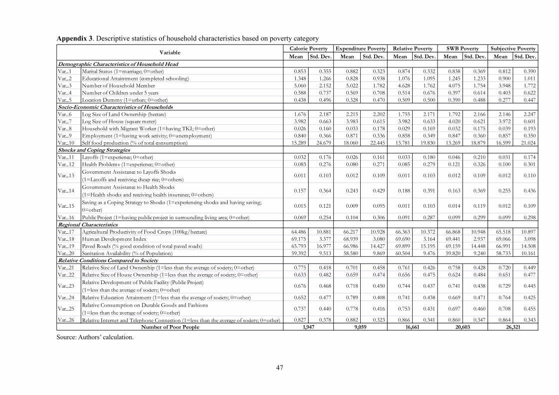
47
Appendix 3. Descriptive statistics of household characteristics based on poverty category
Mean Std. Dev. Mean Std. Dev. Mean Std. Dev. Mean Std. Dev. Mean Std. Dev.
Var_1 Marital Status (1=marriage; 0=other) 0.853 0.355 0.882 0.323 0.874 0.332 0.838 0.369 0.812 0.390Var_2 Educational Attaintment (completed schooling) 1.348 1.266 0.828 0.938 1.076 1.095 1.245 1.233 0.900 1.011Var_3 Number of Household Member 5.060 2.152 5.022 1.782 4.628 1.762 4.075 1.754 3.948 1.772Var_4 Number of Children under 5 years 0.588 0.737 0.569 0.708 0.514 0.676 0.397 0.614 0.403 0.622Var_5 Location Dummy (1=urban; 0=other) 0.438 0.496 0.328 0.470 0.509 0.500 0.390 0.488 0.277 0.447
Var_6 Log Size of Land Ownership (hectare) 1.676 2.187 2.215 2.202 1.755 2.171 1.792 2.166 2.146 2.247Var_7 Log Size of House (square meter) 3.982 0.663 3.983 0.615 3.982 0.633 4.020 0.621 3.972 0.601Var_8 Household with Migrant Worker (1=having TKI; 0=other) 0.026 0.160 0.033 0.178 0.029 0.169 0.032 0.175 0.039 0.193Var_9 Employment (1=having work activity; 0=unemployment) 0.840 0.366 0.871 0.336 0.858 0.349 0.847 0.360 0.857 0.350Var_10 Self food production (% of total consumption) 15.289 24.679 18.060 22.445 13.781 19.830 13.269 18.879 16.599 21.024Shocks and Coping StrategiesVar_11 Layoffs (1=experience; 0=other) 0.032 0.176 0.026 0.161 0.033 0.180 0.046 0.210 0.031 0.174Var_12 Health Problems (1=experience; 0=other) 0.083 0.276 0.080 0.271 0.085 0.279 0.121 0.326 0.100 0.301
Var_13 Government Assistance to Layoffs Shocks(1=Layoffs and receiving cheap rice; 0=others)
0.011 0.103 0.012 0.109 0.011 0.103 0.012 0.109 0.012 0.110
Var_14 Government Assistance to Health Shocks(1=Health shocks and receiving health insurance; 0=others)
0.157 0.364 0.243 0.429 0.188 0.391 0.163 0.369 0.255 0.436
Var_15 Saving as a Coping Strategy to Shocks (1=experiencing shocks and having saving;0=other)
0.015 0.121 0.009 0.095 0.011 0.103 0.014 0.119 0.012 0.109
Var_16 Public Project (1=having public project in surrounding living area; 0=other) 0.069 0.254 0.104 0.306 0.091 0.287 0.099 0.299 0.099 0.298
Var_17 Agricultural Productivity of Food Crops (100kg/hectare) 64.486 10.881 66.217 10.928 66.363 10.372 66.868 10.948 65.518 10.897Var_18 Human Development Index 69.175 3.377 68.939 3.080 69.690 3.164 69.441 2.937 69.066 3.098Var_19 Paved Roads (% good condition of total paved roads) 65.793 16.977 66.986 14.427 69.899 15.195 69.159 14.448 66.991 14.508Var_20 Sanitation Availability (% of Population) 59.392 9.513 58.580 9.869 60.504 9.476 59.820 9.240 58.733 10.161
Var_21 Relative Size of Land Ownership (1=less than the average of society; 0=other) 0.775 0.418 0.701 0.458 0.761 0.426 0.758 0.428 0.720 0.449Var_22 Relative Size of House Ownership (1=less than the average of society; 0=other) 0.633 0.482 0.659 0.474 0.656 0.475 0.624 0.484 0.651 0.477
Var_23 Relative Development of Public Facility (Public Project)(1=less than the average of society; 0=other)
0.676 0.468 0.718 0.450 0.744 0.437 0.741 0.438 0.729 0.445
Var_24 Relative Education Attainment (1=less than the average of society; 0=other) 0.652 0.477 0.789 0.408 0.741 0.438 0.669 0.471 0.764 0.425
Var_25 Relative Consumption on Durable Goods and Fashions(1=less than the average of society; 0=other)
0.737 0.440 0.778 0.416 0.753 0.431 0.697 0.460 0.708 0.455
Var_26 Relative Internet and Telephone Connection (1=less than the average of society; 0=other) 0.827 0.378 0.882 0.323 0.866 0.341 0.860 0.347 0.864 0.34316,661 20,603 26,321Number of Poor People 1,947 9,059
Relative Conditions Compared to Society
Regional Characteristics
VariableCalorie Poverty Expenditure Poverty
Demographic Characteristics of Household Head
Socio-Economic Characteristics of Households
Relative Poverty SWB Poverty Subjective Poverty
Source: Authors’ calculation.

48
Appendix 4. Cross correlation matrix
Y1 Y2 Y3 Y4 Y5 Var_1 Var_2 Var_3 Var_4 Var_5 Var_6 Var_7 Var_8 Var_9 Var_10 Var_11 Var_12 Var_13 Var_14 Var_15 Var_16 Var_17 Var_18 Var_19 Var_20 Var_21 Var_22 Var_23 Var_24 Var_25 Var_26Y1 1Y2 0.193 1Y3 0.115 0.464 1Y4 0.009 0.057 0.109 1Y5 0.036 0.240 0.208 0.143 1Var_1 0.004 0.042 0.048 -0.014 -0.077 1Var_2 -0.012 -0.186 -0.163 -0.102 -0.341 0.135 1Var_3 0.109 0.241 0.215 0.026 -0.032 0.335 0.048 1Var_4 0.063 0.132 0.138 0.023 0.036 0.188 0.108 0.367 1Var_5 0.010 -0.069 0.120 -0.030 -0.233 -0.038 0.358 0.005 -0.006 1Var_6 -0.007 0.086 -0.001 0.011 0.151 0.036 -0.207 0.022 0.015 -0.456 1Var_7 -0.012 -0.026 -0.040 -0.004 -0.069 0.008 0.016 0.011 -0.025 0.016 0.059 1Var_8 -0.007 -0.001 -0.014 -0.007 0.025 -0.004 -0.075 -0.017 -0.012 -0.058 0.014 0.013 1Var_9 -0.011 0.011 -0.006 -0.029 -0.012 0.306 0.088 0.135 0.117 -0.083 0.076 -0.002 -0.034 1Var_10 0.032 0.138 0.058 0.048 0.216 -0.072 -0.268 -0.056 -0.025 -0.313 0.247 -0.043 0.053 -0.052 1Var_11 0.007 0.003 0.031 0.093 0.032 0.003 0.015 0.021 0.008 0.040 -0.034 -0.007 0.009 -0.068 -0.015 1Var_12 0.010 0.017 0.037 0.141 0.104 -0.055 -0.094 -0.021 -0.025 -0.025 0.009 0.004 0.015 -0.122 0.083 0.092 1Var_13 0.002 0.009 0.005 0.016 0.021 0.000 -0.014 0.006 0.000 -0.008 -0.015 -0.009 0.003 -0.006 0.002 0.100 0.036 1Var_14 0.014 0.137 0.102 0.066 0.314 -0.044 -0.175 0.019 0.018 -0.111 0.045 0.002 0.033 -0.022 0.110 0.004 0.077 0.020 1Var_15 0.003 -0.014 -0.011 0.009 -0.007 -0.003 0.028 0.001 -0.008 0.036 -0.024 0.030 0.007 -0.007 -0.009 0.039 0.047 0.117 -0.001 1Var_16 -0.017 0.011 -0.012 0.006 0.006 0.016 -0.030 0.007 -0.003 -0.049 0.028 0.032 0.010 0.019 0.039 0.021 0.057 0.015 0.033 0.022 1Var_17 -0.037 -0.018 -0.019 0.012 -0.094 -0.033 -0.055 -0.114 -0.096 0.087 -0.164 0.179 0.054 -0.063 -0.090 0.003 -0.001 0.008 -0.007 0.004 0.062 1Var_18 -0.028 -0.097 0.012 -0.046 -0.164 -0.009 0.172 -0.034 -0.046 0.222 -0.127 0.074 -0.122 -0.008 -0.257 0.008 -0.037 -0.013 -0.119 0.006 -0.002 0.039 1Var_19 -0.047 -0.073 0.015 -0.019 -0.150 -0.036 0.069 -0.116 -0.091 0.230 -0.250 0.038 0.028 -0.046 -0.211 0.012 -0.013 -0.015 -0.066 0.016 0.001 0.515 0.375 1Var_20 -0.011 -0.060 0.035 -0.011 -0.111 -0.001 0.134 0.015 -0.010 0.151 -0.091 0.060 -0.102 0.015 -0.117 0.006 -0.030 -0.008 -0.076 0.002 0.010 -0.072 0.660 0.166 1Var_21 0.006 -0.058 -0.001 -0.006 -0.084 -0.025 0.136 -0.005 -0.003 0.266 -0.749 -0.084 -0.004 -0.052 -0.154 0.024 0.001 0.011 -0.025 0.011 -0.020 0.071 0.059 0.149 0.043 1Var_22 0.001 0.024 0.031 -0.011 0.035 -0.002 -0.030 -0.015 0.001 0.009 -0.091 -0.650 -0.005 0.001 -0.009 0.001 -0.008 0.009 0.010 -0.023 -0.003 0.002 0.008 0.014 -0.003 0.102 1Var_23 -0.028 -0.025 -0.001 -0.004 -0.030 -0.003 0.030 -0.020 -0.009 0.081 -0.108 0.018 0.026 -0.021 -0.077 0.014 0.009 0.007 -0.002 0.014 0.007 0.134 0.065 0.167 0.048 0.071 0.007 1Var_24 0.013 0.146 0.155 0.076 0.259 -0.119 -0.799 -0.022 -0.111 -0.161 0.120 -0.010 0.043 -0.080 0.190 -0.005 0.075 0.004 0.133 -0.016 0.010 -0.001 -0.086 -0.026 -0.065 -0.080 0.026 -0.021 1Var_25 0.017 0.075 0.076 0.004 0.025 -0.001 -0.054 -0.005 -0.009 0.004 -0.013 -0.102 0.002 -0.007 -0.008 -0.001 -0.003 0.014 0.012 -0.014 0.004 0.036 0.025 0.042 0.013 0.024 0.123 0.026 0.052 1Var_26 -0.016 0.028 0.014 0.004 0.015 0.002 -0.115 -0.034 -0.022 -0.114 0.054 -0.150 0.017 0.009 -0.018 -0.009 0.012 0.015 0.024 -0.012 0.040 0.161 0.036 0.089 -0.006 -0.045 0.162 0.013 0.059 0.130 1
Source: Authors’ calculation.

49
Appendix 5. Spearman’s rank correlations among provincial rankings of poverty measurements
Correlation CaloriePoverty
ExpenditurePoverty
RelativePoverty
SWBPoverty
SubjectivePoverty
Calorie 1
Expenditure 0.381 10.038**
Relative Poverty 0.230 0.236 10.222 0.210
SWB Poverty -0.191 -0.015 -0.233 10.312 0.940 0.216
Subjective Poverty 0.211 0.758 0.115 0.198 10.262 0.000*** 0.547 0.295
Note: ** and *** are significant at 5% and 1%, respectively. Figures in italics are p-values. Source: Authors’ calculation.

50
Abstract (in Japanese)
要約
Post-MDGs の開発議論を睨んで、世界では今、「貧困」の概念議論や、満足度、幸福度等を
用いた政策分析•採用に関する議論がたけなわである。「貧困」の概念や捉え方は多様であり、
またそれらは固定化されたものではなく時とともに変化するものでもある。異なる社会経済規
範を有する諸国においてそれらは異なり、同じ社会や国家に於いても経済や社会の発展に伴い
変容する。開発の初期段階において諸国は絶対的貧困と立ち向かうが、1人当たりの所得が高
まってくるにつれ、人々は相対的貧困(格差)や主観的貧困(満足度や幸福度の概念を含む)
をより考える様になると思われる。本論文は、絶対的貧困(カロリー摂取、消費額基準)と相
対的貧困(所得格差)、およびこれら客観的貧困と主観的貧困を計る諸指標とをそれぞれ対比
させつつ構築提示し、それら諸指標の間の関係、各指標で計られた「貧困」の決定要因を探っ
ている。インドネシアをケース国としてその2005年の全国社会経済調査(Susenas)を用
いて分析した結果、1人当たりの消費額を用いた貧困率(14.5%)と主観的貧困率(42%)の間には
28 パーセント近い隔たりがあることがわかった。それは重要な一面ではあるが、客観的•物質
的に貧困でないことは、主観的に貧困でない事の十分条件でもなく、また必要条件でもないこ
とも分析結果は示している。
絶対的貧困指標から主観的指標に至る5種類の貧困指標を構築し、インドネシアの各地域の
各指標によるランク付けを行うと、それらランキングの間には有為な相関がないことがわかる。
貧困の中身•構成は各地域特有なものが多く、貧困削減政策が各地域に合った形でテイラー•メ
イドされている必要が浮かび上がる。Logit および Ordered-Logit モデル推計から得られた結
果は、諸指標で計った「貧困」の決定要因としては、教育達成度、家計サイズ(人数)、不動
産の所有度(農地や家屋を含む)、外国への出稼ぎ労働者の有無、一時帰休や失職などの経済
的ショックの有無、病気等の健康ショックの有無、公共サービスや公共プロジェクトの有無、
道路インフラ等へのアクセス等が重要であることを示している。
教育の効果については特に重要な発見がある。教育無しから初等教育完結、初等教育から中
等教育完結へと教育達成度が1段階向上する度に、5つの貧困指標のどれにおいても「貧困で
ない」とされる確立は11パーセントずつ向上するという結果が得られた。更に重要なことが、
相対的貧困分析が示す結果から見いだされている。物理的資産や耐久消費財の消費レベルが居
住する社会の平均より低いことは(格差が大きいことは)住民の相対的および主観的貧困度を
増すことが示されるが、教育達成度については正の外部性(positive externality)が確認され
る。即ち、人々は教育水準の高い社会に居住することによってより「貧困でない」と感じるの
である。教育は正に人造り、国造りの中心にある。
分析結果はまた、絶対的貧困と相対的貧困の双方への働きかけを考えるのであれば、貧困削
減プログラム(公共投資や ODA によるインフラ整備等も含む)の実施において、対象となる地
域や住民とそうでない地域や住民の双方への配慮が重要であるという政策含意も示している。
地域をまたがって住民を繋ぐこと、正の開発効果が他地域へ波及しやすくする配慮を怠らない
ことが肝要であることを分析結果は示している。
本論文が、今後の多様化する「貧困」議論や「開発」議論に一石を投じることとなれば、そ
れは著者にとって望外の喜びである。


