Aalborg Universitet

Modeling Wireless Sensor Networks for Monitoring in Biological Processes

Nadimi, Esmaeil

Publication date:2008

Document VersionPublisher's PDF, also known as Version of record

Link to publication from Aalborg University

Citation for published version (APA):Nadimi, E. (2008). Modeling Wireless Sensor Networks for Monitoring in Biological Processes. Aalborg:Department of Control Engineering, Aalborg University.

General rightsCopyright and moral rights for the publications made accessible in the public portal are retained by the authors and/or other copyright ownersand it is a condition of accessing publications that users recognise and abide by the legal requirements associated with these rights.

? Users may download and print one copy of any publication from the public portal for the purpose of private study or research. ? You may not further distribute the material or use it for any profit-making activity or commercial gain ? You may freely distribute the URL identifying the publication in the public portal ?

Take down policyIf you believe that this document breaches copyright please contact us at vbn@aub.aau.dk providing details, and we will remove access tothe work immediately and investigate your claim.

Downloaded from vbn.aau.dk on: april 05, 2019

Modeling wireless sensor networks for monitoring in biological processes

Ph.D. thesis

Esmaeil Shahrak Nadimi

Department of Electronic Systems Section for Automation and Control

Aalborg University Fredrik Bajers Vej 7, 9220 Aalborg East, Denmark

Modeling wireless sensor networks for monitoring in biological processes Ph.D. thesis ISBN 978-87-90664-39-8 April 2008

Copyright 2005–2008 (c) Esmaeil Shahrak Nadimi

III

Preface This thesis is submitted as partly fulfillment of the requirements for the Doctor of Philosophy at the Section of Automation and Control, Department of Electronic Systems, Aalborg University, Denmark. The work has been carried out in the period February 2005 to April 2008 under the supervision of Professor Thomas Bak and Senior Scientist Henning Tangen Søgaard.

Aalborg University, April 2008

Esmaeil Shahrak Nadimi

V

Abstract

Modeling wireless sensor networks for monitoring in biological processes

Successful grazing in developed agriculture calls for automated and

efficient monitoring and control of animals. Monitoring should allow us to develop methodologies for detecting individuals with potential health problems, and for optimizing the grazing process (e.g. grazing time budget), which potentially would have a significant impact on practical farming. Management and control of a herd of animals relies on monitoring the herd, which is very complicated due to the geographical distribution of the animals in outdoor environments, as their behavior is strongly governed by their instincts and needs for feed resources. Animal behavior monitoring systems in outdoor environments should be able to remotely register relevant behavioral parameters, as the use of wired sensors is impractical. In this thesis, a ZigBee based wireless sensor network was employed as monitoring system to register the behavior of a group of dairy cows in a herd. Only a part of the herd was monitored, as monitoring each individual animal in a large herd under practical conditions is inefficient in terms of costs. Investigations to show that the monitored animals can indeed represent the whole herd were carried out. The tagged animals in the herd were equipped with wireless nodes around the neck capable of measuring two behavioral parameters: the pitch angle of the neck (using accelerometer) and the velocity of the movement of the animal (using received signal strength). Fusing the two measured behavioral data resulted in an improvement of the classification results regarding the animal behavior mode (activity/inactivity), compared to the results achieved by only monitoring one of the behavioral parameters. Applying a multiple-model adaptive estimation (MMAE) approach to the data resulted in the highest classification success rate in comparison to other classification approaches (such as decision tree, fuzzy logic classifier and neural network), due to the use of precise forth-order mathematical models which relate the feed offer as input to the pitch angle of the neck as the output of the model.

This thesis shows that wireless sensor networks can be successfully employed to monitor the behavior of a herd of dairy cows in outdoor environments. The approaches used in this thesis can be extended to a variety of applications in animal behavior monitoring, modeling and classification. The

VI

proposed models describing animal behavior modes can be used to control the behavior of herds of animals in terms of the activity of the animals.

VII

Synopsis

Vellykket græsning i moderne landbrug kræver automatisering og effektiv monitorering og styring af dyrene. Monitoreringen skal sætte os i stand til at udvikle metoder til detektering af potentielt sygdomsramte enkeltdyr samt at optimere af græsningsprocessen (fx tidsbudgettet for græsningen), som kan have betydelig indflydelse på praktisk landbrug. Styring og kontrol af en flok dyr er afhængig af en monitorering af flokken, hvilket er meget kompliceret pga. den geografiske fordeling af dyrene i udendørs omgivelser, idet deres adfærd er stærkt styret af deres instinkter og behov for foder. Systemer til monitorering af dyrs adfærd i udendørs omgivelser skal kunne foretage en fjernregistrering af relevante adfærdsparametre, da anvendelsen af trådede sensorer er upraktisk.

I denne afhandling er der anvendt et ZigBee-baseret trådløst sensornetværk som monitoreringssystem til registrering af en gruppe malkekøers adfærd. Kun en del af flokken blev monitoreret, da monitorering af hvert enkelt dyr i en stor flok under praktiske forhold er omkostningsmæssigt ineffektiv. Der blev gennemført undersøgelser, der skulle vise, at de monitorerede dyr var repræsentative for hele flokken. De mærkede dyr i flokken blev udstyret med trådløse enheder fæstnet omkring halsen. Enhederne var i stand til at måle to adfærdsparametre: halsens hældningsvinkel (ved brug af accelerometer) og dyrenes bevægelseshastighed (baseret på signalstyrken). Kombination af de to typer af adfærdsdata resulterede i en forbedring af klassifikationsresultaterne mht. dyrenes adfærdstype (aktiv/inaktiv) i forhold til resultater opnået ved kun at monitorere en af adfærdsparametrene. Ved anvendelse af model adaptive estimation (MMAE) blev der opnået en klassifikation med højere succesrate end med andre klassifikationsmetoder (fx decision tree, fuzzy logic classifier and neurale netværk), pga. brugen af en præcis fjerdeordens matematisk model, som knytter fodermængden som input til halsens hældningsvinkel som output af modellen. Denne afhandling viser, at trådløse sensornetværk kan anvendes med succes til monitorering af en flok malkekøers adfærd i udendørs omgivelser. Metoden, der anvendes i denne afhandling, kan udvides til en række anvendelser vedrørende monitorering af dyrs adfærd samt til modellering og klassifikation. De fremsatte modeller til beskrivelse af dyrs adfærdstyper kan anvendes til at styre en dyrefloks adfærd mht. dyrenes aktivitet.

IX

Acknowledgments I would like to appreciate my supervisors Thomas Bak and Henning Tangen Søgaard for their continuous support and guidance during the past three years and for their great help. Thomas has been a great help in guiding and showing me the correct route to achieve the final goal of the project with his scientific vision. A special acknowledgment is due to the time dedication of Henning to the project. Without his many hours working and being in touch whenever I needed him, the project would not be accomplished. Thanks! Very special thanks go to my former supervisor Roozbeh Izadi-Zamanabadi for many great discussions of different ideas over the years. Without him, definitely the project could not be accomplished. I would like to thank everyone, students as well as colleagues at Research Center Bygholm, Aarhus University and others, who have helped at field tests and their support. Special thanks to my friends at Aalborg University. Without their help whenever I was in Aalborg, this thesis could not come to an end. I would like here to thank my family, especially my parents who supported me in any condition during my whole life. I really appreciate that they have always trusted me. Thanks! Finally the greatest acknowledgment goes to Victoria for her support and patience during these three years, and the happiness and motivations that she has dedicated me.

XI

Contents I Introduction 1.1 Motivation and background...……………………………………….............9 1.2 Previous work..…………………………………………………….............12 1.3 Contributions………………………………………………………............21 1.4 Thesis outline……………………………………………………................22 References………………………………………………………………...........24 II Monitoring Cow Behavior Parameters based on Received Signal Strength using Wireless Sensor Networks Abstract..…………………………………………………………….................30 2.1 Introduction..………………………………………………………............30 2.2 Problem statement and background......……………………………...........31 2.4 Materials and methods..……………………………………………............33 2.5 Experimental setup and results…………………………………….............38 2.6 Conclusions………………………………………………………...............39 References………………………………………………………………...........40 III ZigBee-based wireless sensor networks for monitoring animal presence and pasture time in a strip of new grass Abstract..………………………………………………………….....................44 3.1 Introduction..………………………………………………………............45 3.2 Materials and methods......…………………………………………...........48 3.3 Experimental setup and results......…………………………………...........57 3.4 Conclusions..………………………………………………………............62 References………………………………………………………………...........65 IV ZigBee based Wireless Sensor Networks for classifying the behavior of a herd of animals using classification trees 4.1 Abstract...………………………………………………………….............70 4.2 Introduction………………………………………………………..............70 4.3 Problem statement and background......……………………………...........72

CONTENTS

XII

4.4 Materials and methods..……………………………………………...........74 4.5 Results……………………………………………………………..............88 4.6 Conclusions………………………………………………………..............89 4.7 References………………………………………………………................90 V Observation Kalman filter identification and multiple-model adaptive estimation for classifying animal behavior using wireless sensor networks Abstract……………………………………………………………...................94 5.1 Introduction………………………………………………………..............95 5.2 Observer Kalman filter identification method.....…………………............97 5.3 Multiple-model adaptive estimation approach……………………...........101 5.4 Experimental setup and results……………………………………...........103 5.5 Conclusions………………………………………………………............112 References…………………………………………………………….............112 VI Conclusions, discussions and future works 6.1 Conclusions………………………………………………………............116 6.2 Future work................................................................................................119 Appendixes............................................................................................121 Bibliography ...................................................................................................143 Published and submitted papers...................................................................149

CONTENTS

1

Nomenclature Chapter 2 k time instant −kx̂ a priori state estimate

kx̂ a posteriori state estimate −

kP a priori estimate of error variance

kP a posteriori estimate of error variance

kK Kalman gain

kQ process noise covariance

kR measurement noise covariance

kγ arrival sequence

kw process noise

kv measurement noise

kH output matrix

kϕ system matrix

θ pitch angle of the neck

TxP transmitted power levels

RxP received power levels

TxG antenna gains of the transmitter

RxG antenna gains of the receiver λ wavelength d distance between transmitter and receiver

n attenuation factor

CONTENTS

2

α optimal antenna gain

Chapter 3

TxP transmitted power levels

RxP received power levels d distance between transmitter and receiver C optimal antenna gain

)(tγ packet arrival sequence K,2,1=t time

WL window length

T threshold )(tγ ′ filtered packet arrival sequence

0r gateway connectivity range )(te classification error )(ˆ tr RSS based estimate of the distance between a node and

gateway Δ extended area

ET pasture time in the extended area

CT pasture time in the gateway connectivity area

K ratio of the extended area to the gateway connectivity area

1D number of monitored cows in the extended

2D total number of cows in the extended area k ratio between total number of cows and number of

monitored cows 0H null hypothesis

1H alternative hypothesis

CONTENTS

3

1μ theoretical mean values of 1D

2μ unknown mean value of 2D

1σ theoretical standard deviation of 1D

2σ unknown standard deviation of 2D α significance level

v degrees of freedom

0t t-statistics

1y sample means of 1D

2y sample means of 2D

1s Sample standard deviation of 1D

2s Sample standard deviation of 2D

1n sample size for 1D

2n sample size for 2D

Chapter 4 k time instant −kx̂ a priori state estimate

kx̂ a posteriori state estimate −

kP a priori estimate of error variance

kP a posteriori estimate of error variance

kK Kalman gain

kQ process noise covariance

kR measurement noise covariance

kγ arrival sequence

CONTENTS

4

kx true (unknown) state

kz RSS measurements or acceleration measurements

kw process noise

kv measurement noise

kH output matrix

kϕ system matrix

cλ critical value for arrival probability of the observation update

λ lower bound of arrival probability of the observation update

λ upper bound of arrival probability of the observation update p maximum eigenvalues of the system matrix

)(0 ⋅I zero order modified Bessel function of the first kind α real parameter which determines the shape of the window N window length

TxP transmitted power levels

RxP received power levels

TxG antenna gains of the transmitter

RxG antenna gains of the receiver

WLλ wavelength d distance between transmitter and receiver

en attenuation factor

C optimal antenna gain

kd distance between the cow node and the gateway

kD change in distance during each sampling interval a cow number q day number

CONTENTS

5

aqT training dataset '

aqT validation dataset

Chapter 5 k time instant

)(ku input vector )(ky output vector )(kx state vector

A system dynamic matrix

B input matrix C output matrix

D G observer gain matrix

)(kv extended input vector

A extended system dynamic matrix

P prediction horizon

Y set of L predicted output values

L number of data points

V extended input matrix θ vector of observer Markov parameters

+V pseudo-inverse of V ss integer n state vector dimension

R unitary left matrix

CONTENTS

6

S unitary right matrix ∑ rectangular matrix of singular values

n∑ controllable and observable system singularvalues )(sH transfer function of the true system

nR first n columns of R

nS first n columns of S

M general model in MMAE approach )(kμ probability that the MMAE method attributes to

model M ),,( 0 kk yyY K= Measurement up to time instant k

)(kjλ probability that a model is correct

)(ky observation data

)(krj residual measurements

jS covariance matrix

W window length

CHAPTER 1

Introduction

Section 1.1: Motivation and background

8

This thesis is the result of a three year study of animal (dairy cow)

behavior monitoring and modeling, which began in February of 2005 aimed at developing an autonomous monitoring system capable of registering the behavior of a group of dairy cows using wireless sensor networks. The thesis documents innovations in the areas of system architecture, wireless sensor network implementation, mathematical modeling and system identification related to animal behavior monitoring.

This thesis addresses monitoring and modeling animal behavior in terms of activity and inactivity in outdoor environments. Several studies have focused on animal behavior monitoring and control inside the barn, but new challenges are introduced in outdoor environments, where the habitat areas are larger and where the animals are more dynamic. Designing a monitoring system capable of remotely registering animal behavior prevents potential disturbances on the animal behavior, and is important for animal science studies. It may also help to provide a better environment for the animals to live in while optimizing their production.

The main objectives of this thesis are as follows: 1) Selecting relevant behavioral parameters that by monitoring and

analysis allow different behavioral modes (e.g. activity or inactivity) to be detected.

2) Providing a monitoring system that can measure and monitor the behavioral parameters.

3) Classify behavioral modes such as active or inactive. A comparison can then be made between different behavioral modes of monitored animals and productive animals. For instance, the time length that each individual animal spends in a specific behavioral mode (e.g. active) can be compared with the same time of a high productive animal. This comparison can be used as a basis for adjustment of the behavioral modes of the low-productive animals.

In this thesis, pitch angle of the neck and the translational velocity of the animal were selected as behavioral parameters based on the fact that when an animal is active (grazing or searching for feed), its neck is down and the velocity is nonzero, and when inactive (lying down or ruminating), the neck is horizontal and the velocity is zero.

To classify the behavior into various modes such as active or inactive, different classification approaches such as decision trees, fuzzy logic classifiers, neural network classifiers and a Multiple-Model Adaptive Estimation approach (MMAE) were applied to the data.

Chapter 1

9

1.1. Motivation and background

Public perception, animal welfare and milk quality call for a continued use of grasslands for grazing in dairy farming (Torjusen et al., 2001). To meet the public concern, some milk producers offer incentives to dairy farmers if they let their dairy cows graze outdoor, but for many farmers this is impossible due to livestock management and control problems. Management and control relies on monitoring the herd, which is significantly complicated by the inherent geographical distribution of the animals in outdoor environments. The distribution and the behavior of the animals are mainly governed by their needs for feed resources and water.

Successful grazing in developed agriculture calls for automated and efficient monitoring and control of animals. The monitoring should allow us to establish a better understanding of animal behavior, to detect individuals with potential health problems, and generally to optimize the grazing process (e.g. grazing time budget). All things that potentially would have significant impacts on practical farming. An important example is the interaction between animals and their feed supply. Sustainable management of grassland systems requires understanding of the impact of grazing livestock on the vegetation. Behavioural models may provide this understanding by accurately modeling feeding patterns, meal consumption and timing to predict total feed intake (ASAB, 2008).

Feed offer has fundamental impact on the production of the animals. If the feed offered to the animals is below a certain amount, their production will be affected. This situation can be detected by monitoring the behavior of the animals. For instance, if the feed offered to the animals is low, the eating time length decreases, as they will spend more time looking for feed. Therefore, the relation between the different animal behavioral modes (such as eating or lying down) and their production can be achieved by registering daily time budget as exemplified in Table 1.

Table 1. Sample daily time budget for dairy cows (milk production association, 2005)

Daily time budget for dairy cows

Daily behavioral time budget for top-10% of cows by milk production

Activity Time devoted to activity per day

Activity Top 10% average

Eating 3 to 5 h (9 to 14 meals / day) Eating 5.5 h Lying/resting 12 to 14 h Resting 14.1 h

Social interactions 2 to 3 h Standing 1.1 h Ruminating 7 to 10 h Perching 0.5 h

Drinking 30 min Drinking 20 min

Section 1.1: Motivation and background

10

Once the time budget table is obtained for each individual animal, its behavioral modes and production can be compared to the behavioral modes and the production of the high-productive animals of the farm. In the example shown in Table 1, the normal eating time length of an individual dairy cow was between 3 to 5 hours per day, while the top 10% productive animals of the farm ate 5.5 hours per day. Knowledge of the individual time budgets is the basis for actions to bring the under performers into a situation where they perform better. Monitoring animal behavior in terms of activity can potentially be used as input to a control system for controlling the behavior by adjusting for example the environment, to optimize behavior relevant for productivity. Registration of the automatic monitoring system may also help to reveal individuals with health problems and behavior abnormalities through identification of deviations from normal behavior.

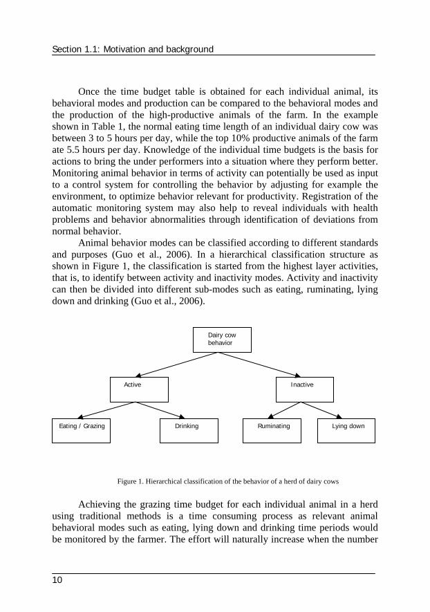
Animal behavior modes can be classified according to different standards and purposes (Guo et al., 2006). In a hierarchical classification structure as shown in Figure 1, the classification is started from the highest layer activities, that is, to identify between activity and inactivity modes. Activity and inactivity can then be divided into different sub-modes such as eating, ruminating, lying down and drinking (Guo et al., 2006).

Figure 1. Hierarchical classification of the behavior of a herd of dairy cows Achieving the grazing time budget for each individual animal in a herd

using traditional methods is a time consuming process as relevant animal behavioral modes such as eating, lying down and drinking time periods would be monitored by the farmer. The effort will naturally increase when the number

Dairy cow behavior

InactiveActive

Eating / Grazing Lying down RuminatingDrinking

Chapter 1

11

of animals and the spatial distribution increases (i.e. inside the barn or in an outdoor environment). Manual registration of such a time budget may also potentially disturb the behavior of the animals and as a consequence, in the worst case, the productivity of the animal can significantly decrease (Szewczyk et al., 2004).

Consequently, autonomous monitoring system capable of registering relevant animal behavior is desirable. The monitoring system should be able to precisely monitor the behavior of each individual animal without disturbing their behavior. The monitoring system should be robust and flexible enough in order to function in a rough environment such as e.g. fields covered by trees.

In general, animal behavior monitoring systems should be able to remotely register relevant behavioral parameters using wireless communication. In practice, the use of wired sensors to monitor animal behavior is completely impractical due to their natural mobility. Animal behavior monitoring systems that are based on RFID tags are short range wireless sensors, which make them rather impractical in the large fields. In order to be able to monitor the behavior of a herd of animals across a whole field using RFID tags, extra infrastructure facilities such as large number of aggregation points (gateways) are required.

Behavioral parameters such as pitch angle of the neck can not be monitored and sensed by the off-the-shelf RFID based monitoring systems. On the contrary, the translational velocity can be indirectly estimated from the location of the wireless nodes (associated with each cow) monitored using grid topology localization approach (Ramadurai et al., 2005). In the grid approach, the network space is divided into a uniform grid and the probability of node presence is estimated at each square of the grid. The main drawback of this method is the need of covering each square of the grid by a gateway. The finer and more accurate the grid is, the higher number of gateways are needed.

Other animal behavior monitoring systems based on Bluetooth or WiFi are practical in outdoor environments and large fields but high energy consumption and long network joining time are their main drawbacks. Therefore, a low-cost low-power monitoring system that can fulfill the requirements (such as the ability to handle a large number of nodes per network, the ability to identify new incoming wireless nodes without the necessity of restarting the whole network) is needed.

The monitoring system which is the basis for this dissertation benefits from a ZigBee based wireless sensor network. It is a low cost system that is equivalent to Bluetooth or WiFi based monitoring systems with mesh networking capability, with lower power consumption, shorter network joining times, higher networking capability and with a relatively long range of

Section 1.2: Previous work

12

communication (in outdoor environments) and with self healing and self configuring characteristics.

1.2. Previous work This section will address previous work related to topics that is essential for this dissertation. The topics include: 1.2.1. Behavior parameter monitoring

Various behavioral parameters of different animals have been studied by different researchers aimed at achieving more information and deeper insight about the behavior of animals under different conditions. This knowledge can potentially help animal behavior experts to interpret the behavior and consequently predict the animal behavior under certain conditions, such as when the animal is in lack of feed, lack of light or under heat stress. For instance, the behavior of groups of seabirds under different conditions was monitored and studied by Szewczyk et al., (2004). The time period that each seabird spent in the nest in different conditions was monitored by a large network of wireless sensors in which the temperature and the light of each nest was used as the indicator of bird presence inside the nest.

Combining cameras and distributed, non-invasive sensors with elements of computer vision, information technology and artificial intelligence, enabled monitoring the effect of new medicine on the behavior of a group of mice in the lab (Belongie et al., 2004). The behavior and habits of honeybees and wasps were tracked by radio frequency identification (RFID) tags in a wireless sensor network in the research carried out by Roberts et al., (2004).

The spatial distribution of a herd of dairy cows in the barn or in the field were tracked and monitored by White et al., (2001), Butler et al., (2004), Munksgaard et al., (2005), Braunreiter et al., (2007), Maertens et al., (2007), Umstatter et al., (2006), and Schwager et al., (2007). The velocity of the movements of animals in the field were monitored and registered by Oudshoorn et al., (2006) based on both positions and the velocities of the movements in the field. Different behavior modes of dairy cows such as standing and lying down when they were in the barn were evaluated by Munksgaard et al., (2005), Wilson et al., (2005) and Sallvik et al., (2005).

Health parameters such as pH of the rumen was measured and monitored by Mottram et al., (2006) and Lokhorst et al., (2007) while experiments to

Chapter 1

13

measure body temperature using rumen bolus were carried out by Ipema et al., (2006).

1.2.2. Monitoring systems As all these measured behavioral parameters (position, velocity, rumen

PH, and jaw movements) can potentially represent the animal behavior in terms of activity, new perspectives to solve the problem of animal (dairy cow) behavior monitoring in terms of activity were introduced by Umstatter et al., (2006) and Schwager et al., (2007) by measuring the pitch angle of the neck of the animal. It relies on the fact that when the animal is active (grazing or looking for the grass), the head is down (slanted neck) and the translational velocity of the animal is nonzero while in the inactivity mode such as lying down or ruminating, the head is up (horizontal neck) and the velocity of the movement is zero. Consequently, the pitch angle of the neck and the velocity can be indicators of the behavioral mode in terms of animal activity.

In order to measure the behavioral parameters such as position, velocity, pitch angle of the neck and the pH of the rumen, different methods and strategies and consequently different monitoring systems (sensors) have been employed by different researchers. For instance, the position of a herd of dairy cows in the field was monitored and registered using Global Positioning System (GPS) in the experiments carried out by White et al., (2001), Butler et al., (2004), Braunreiter et al., (2007), Maertens et al., (2007), Umstatter et al., (2006), Oudshoorn et al., (2007) and Schwager et al., (2007). By post processing of registered locations from the GPS, the movement velocity was estimated by Oudshoorn et al., (2007). Munksgaard et al., (2005) used received signal strength (RSS) in a wireless sensor network and estimated the translational velocity of a group of dairy cows in a barn. Different behavior modes of dairy cows such as standing and lying down in the barn were evaluated by Munksgaard et al., (2005) using an accelerometer around the leg and a data logger. Sallvik et al., (2005) used video processing combined with a RFSU (radio frequency synchronization unit). Herbivore jaw movements to detect the grazing behavior were monitored by Ungar et al., (2007) using a sound sensor.

Nagl et al. (2003) designed a remote health-monitoring system for cattle that included various sensors, such as a GPS unit, a pulse oximeter, a core body temperature sensor, an electronic belt, a respiration transducer and a temperature sensor. The system communicated wirelessly with a base station via Bluetooth communication protocol. Taylor and Mayer (2004) reported a

Section 1.2: Previous work

14

study regarding a smart and comprehensive animal management system. Each animal was equipped with a wireless node (sensor + mote), which could provide accurate measurements of the location and health-related information of the animal wirelessly. Haapala (2003) tested the performance of radio frequency identification (RFID) tags and various readers (gateway) on cattle under extremely cold temperature in Finland. Brown-Brandl et al. (2001) tested a short-range communication system for measuring core body temperature in poultry, beef and dairy cattle. Temperature transmitters were implanted into the body of the animals. A CorTempTM miniaturized ambulatory logger received the temperature data wirelessly. Test results showed good accuracy, resolution, and response time for temperature measurement. Kononoff et al. (2002) used a wireless automatic system to record the chewing and ruminating behaviors to study the dietary factors affecting normal rumen function of dairy cows. Butler et al. (2004) developed a moving virtual fence algorithm for limiting the movements of a group of dairy cows in predefined boundaries. Each animal in the herd was equipped with a smart collar consisting of a GPS, a PDA, a radio unit (WLAN) and a sound amplifier. The animal’s location was determined using the GPS and was verified through a measurement of proximity of the cow relative to the fence boundary. When the animal approached the perimeter, it was presented with a sound stimulus, which drove the animal away from the fence. The pitch angle of the neck of a group of dairy cows were measured by Schwager et al., (2007) using a magnetometer mounted around the neck of the cow.

1.2.2.1 Sensors Each monitoring system has specific advantages but also problems. GPS

is a relatively precise sensing system to monitor the location of animals, however high energy consumption in addition to frequent connection loss with the satellites in environments covered by trees makes it inefficient for animal behavior monitoring (Oudshoorn et al., 2006; Schwager et al., 2007). Attaching an accelerometer equipped with a data logger to the leg of animals and registering the status of the leg in the experiments carried out by Munksgaard et al., (2005) demonstrated reliable results but the problem is the use of an offline monitoring system. Another drawback of the employed monitoring system by Munksgaard et al., (2005) is that the sensors are attached around the leg of the animal, and as a consequence, the communication with the aggregation point will be lost when the animal lies down. The communication range will also significantly decrease when the sensor is covered by mud. Consequently, online

Chapter 1

15

low cost low power wireless sensor networks as used by Szewczyk et al., (2004) are appropriate. One of the problems introduced in the research carried out by Schwager et al., (2007) was the use of magnetometers for measuring the pitch angle of the neck as the magnetometers saturates easily in the presence of relatively strong magnetic fields. Accelerometers on the other hand are not affected by the saturation problem; the main disadvantage of using them is their sensitivity to temperature variations. The solution to this problem is addressed in this thesis by employing a temperature sensor and calibrating the acceleration measurements. The pitch angle of the neck is estimated from the acceleration data. A rough estimation of the translational velocity of the animal is achieved by post processing the distance estimates measured using received signal strength (RSS).

1.2.2.2 Network In order to aggregate the sensor readings in a wireless sensor network,

different communication protocols such as ZigBee, Bluetooth, WiFi and radio frequency identification (RFID) have been employed in different contributions by Polastre, (2004), Roberts et al., (2004), Butler et al., (2004), Munksgaard et al., (2005), Szewczyk et al., (2004), Schwager et al., (2007), Ipema et al., (2006) and Lokhorst et al., (2007). A brief comparison among the communication protocols are presented by Table 2. All these standards use the instrumentation, scientific and medical (ISM) radio bands, including the sub-GHz bands of 902–928MHz (US), 868–870MHz (Europe), 433.05–434.79MHz (US and Europe) and 314–316MHz (Japan) and the worldwide acceptable GHz bands of 2.400–2.4835 GHz (Wang et al., 2006). Table 2. Comparison between wireless LAN, Bluetooth and ZigBee, (Wang et al., 2006)

Feature WiFi (IEEE 802.11b) Bluetooth (IEEE 802.15.1)

ZigBee (IEEE 802.15.4)

Radio DSSS FHSS DSSS Data rate 11 Mbps 1 Mbps 250 kbps Nodes per master 32 7 64,000 Slave enumeration latency Up to 3 s Up to 10 s 30 ms

Data type Video, audio, graphics, pictures, files

Audio, graphics, pictures, files Small data packet

Range (m) 100 10 70 Extendibility Roaming possible No Yes Battery life Hours 1 week >1 year

Feature WiFi (IEEE 802.11b) Bluetooth (IEEE 802.15.1) ZigBee (IEEE 802.15.4)

Section 1.2: Previous work

16

Using radio signals with a lower frequency leads to a longer transmission range and a stronger capability to penetrate through walls and glass, but the absorption rate will also be higher with lower frequencies. Radio waves with higher frequencies are easier to scatter; therefore effective communication range for signals carried by a high frequency radio wave may not necessarily be shorter than that by a lower frequency carrier at the same power rating.

Bluetooth (IEEE 802.15.1) is a wireless protocol that is used for short-range communication. It uses the 2.4 GHz, 915 and 868MHz radio bands to communicate at 1 Mbit between up to eight devices and was used for localizing a group of dairy cows inside the barn using received signal strength (position by post processing using triangulation) in the research carried out by Munksgaard et al., (2005).

WiFi networks use radio technologies (IEEE 802.11) to provide fast, reliable and secure connectivity. WiFi networks can be used to connect computers to each other, to the internet and to wired networks. WiFi works in unlicensed 2.4 GHz (802.11b/g), and 5 GHz (802.11a/h) with 11 Mbits (802.11b) or 54 Mbits (802.11a/g).

ZigBee (IEEE 802.15.4) is a wireless protocol that is used for low data rate connectivity among relatively simple devices that consume minimal power and typically connect over short distances. It is ideal for monitoring, control, automation, sensing and tracking applications for home, medical and industrial environments and has been used for animal behavior monitoring purposes in the researches carried out by Szewczyk et al., (2004) and Ipema et al., (2006).

After measuring animal behavior parameters using wireless sensors, the behavioral parameters need to be aggregated and sent to infrastructures facilities for further processing. Nodes memory in a wireless sensor network is a very scarce resource because some of the functionalities must be available all the time, therefore, the memory should be used most efficiently. The measured data by wireless node can be potentially processed at the local memory of the node (Szewczyk et al., (2004)), but it should not affect other necessary applications running on the node due to lack of memory.

1.2.3. Classification and behavior modeling Different classification methods to classify animal behavior have been

employed in different studies. A K-means classifier was applied to the data of location and the pitch angle of the neck of a herd of cattle to classify their behavior into two modes, active and inactive, in the research carried out by Schwager et al., (2007) and Guo et al., (2006). Decision trees were applied to

Chapter 1

17

the data of the pitch angle of the neck of a herd of sheep in the investigations of Umstatter et al., (2006). In this thesis, the same approach is applied to the data of the pitch angle of the neck and the velocity of the movement of a group of dairy cows. In addition, a very simple threshold method is used to classify the behavior into two modes as active and inactive. Fuzzy logic and neural network classifiers are also applied to the data of the pitch angle of the neck and the translational velocity. In addition a Multiple-model adaptive estimation (MMAE) approach is applied. In order to detect different behavioral modes and the transition among them (e.g. from activity to inactivity or vice versa) using the MMAE approach, one or several models describing different behavioral modes are required (Ferreira and Waldmann, (2007)). Such a model should be able to simulate the actual animal behavior as precise as possible. Among all the relevant models introduced in the literature able to model behavior of animals, entity and group mobility models received considerable attention due to their simplicity (Camp et al., 2004; Ting et al., 2007; Chang & Liao, 2004; Yoon et al., 2005; Blakely & Lowekamp, 2004; Bai & Helmy et al., 2005; Sommer, 2007). The entity mobility models are classified into two groups defined by a high degree of freedom and a low degree of freedom models respectively (Camp et al., 2004). High degree of freedom mobility models such as random walk, random waypoint, random direction and Gauss-Markov mobility models and low degree of freedom models such as freeway and city section mobility models as described by Camp et al., (2004), Chang & Liao, (2004) and Yoon et al., (2005) are briefly presented below.

1.2.3.1 Random walk mobility model

The random walk mobility model, also known as Brownian motion, was

developed by Einstein to resemble the chaotic movement of entities observed in nature (Camp et al., 2004). In the random walk mobility model, the entity moves from its current location to a new location by randomly choosing a direction and a speed from a predefined range, known as [0,2π] and [minimum-speed, maximum-speed] respectively. A new direction and speed will be chosen either at a constant time interval or after a constant distance being traveled. If the entity reaches the boundary of the area in which is able to move, it will bounce off the border with a predetermined angle (sommer, (2007)).

The random walk mobility model is a memory-less model due to independency of the current speed or direction to the past measurements. This characteristic can generate unrealistic movements such as sudden stops and

Section 1.2: Previous work

18

sharp turns, which infrequently happens in animal behavior science (Oudshoorn et al., 2006).

1.2.3.2 Random waypoint mobility model

The main difference between the random waypoint mobility model and

the random walk mobility model is that pause intervals between changes in speed and direction are included. After the pause interval expires, the entity chooses a new set of coordinates by choosing a random speed and direction (Camp et al., 2004, Sommer et al., 2007, Bai & Helmy et al., 2005).

1.2.3.3 Random direction mobility model

The random direction mobility model performs like the random walk or

random waypoint mobility models; however an entity would only pause and change speed and direction when it hits the border of the area. As opposed to the random walk and random waypoint, the random direction model distributes an entity’s movement equally around the area (Camp et al., 2004, Sommer et al., 2007).

1.2.3.4 Gauss-Markov mobility model

The Gauss-Markov mobility model was designed to vary the level of

randomness of the movement using only one tuning parameter. In this model, each entity is initially assigned a given speed and direction. At fixed time intervals, the speed and direction for each entity are updated and new movements occur. The new speed nS and direction nd at time instance thn is

calculated using the values at time instance thn )1( − and a random variable as described by Eq. (1) (Prabhakaran & Sankar, 2006).

1

1

)1()1(

)1()1(2

1

21

−

−

−+−+=

−+−+=

−

−

n

n

xnn

xnn

dddd

SSSS

ααα

ααα (1)

The variable α is the tuning parameter with the upper and lower limit set

as one and zero respectively ( 10 ≤≤ α ). S and d are constants representing

Chapter 1

19

the mean value of the speed and direction as ∞→n . Finally 1−nxS and

1−nxd are two random variables chosen from a Gaussian distribution. If α is set to zero, the movement is totally random and thereby equivalent to Brownian motion while linear motion is obtained by setting α equal to one. Values between zero and one correspond to different degrees of random movements.

The Gauss-Markov mobility model is capable of reducing the sudden stops or sharp turns encountered in the random walk and the random waypoint mobility models because an entity’s past velocity and direction has been taken into account when a new speed or direction is assigned (Chang & Liao, (2004), Prabhakaran & Sankar, (2006)).

Based on animal behavior studies, a group of dairy cows rarely walk randomly, however, their behavior and their spatial distribution are mainly governed by food resources (Bishop-Hurley et al., 2007; Oudshoorn et al., 2007). The main drawback of representing the behavioral data using random models (Brownian motion) is not considering the influence of feed offer on the behavioral data. Taking into account that the feed offer can strongly affect animal behavior and the input to the random models (e.g. Brownian motion) is white noise, models that can include the effect of feed offer as input on the behavioral modes are preferred. Consequently, in order to estimate the models that could relate the feed offer to the behavioral parameters, different system identification techniques (Ljung, 1988) can be applied to the data representing pitch angle of the neck and the feed offer.

1.2.3.5 Model identification System identification is the process of developing or improving a

mathematical representation of a physical system using experimental data (Juang, 1988). The analysis could be performed in the frequency domain or the time domain. For a long time, frequency domain identification and time domain identification were considered as competing methods to solve the same problem which was building a model for a linear time-invariant (LTI) dynamic system. At the end, the frequency domain achieved a bad reputation because the transformation from time domain to frequency domain is prone to leakage errors where noiseless data in the time domain resulted in noisy frequency response function (FRF) measurements (Zhang et al., 2005). However, it has been shown that exactly the same problem could occur in the time domain. It was also been shown that by extending the models, a full equivalence exist

Section 1.2: Previous work

20

between both domains (Zhang et al., 2005). Once this equivalence between both domains was established, the question was raised whether there is any difference between them. It is important to notice that although both domains carry exactly the same information, it might be simpler to represent the information in one domain compared to the other domain because the same information are represented differently (Zhang et al., 2005).

Among different time domain identification techniques such as correlation analysis, state space modeling, black-box modeling and time series analysis (MATLAB, 2007), state space modeling is widely used (Tiano et al., 2007; Elkaim et al., 2002; Juang, 1988). Robust numerical properties and relatively low computational complexities make the state space model very practical (Elkaim, 2002). Describing a system by a set of first-order differential equations, rather than by one or more thn -order differential equations could be another reason. Another advantage of state space model analysis over other methods is the quick estimation process because only two parameters (the poles and the input delay) must be identified.

Depending on various applications, different types of state space modeling could be utilized. Based on projection techniques in Euclidean space, subspace identification methods (SIMs) have been one of the main topics of research in system identification (Gevers, 2003). Several representative algorithms have been published, including canonical variate analysis (CVA, Larimore, 1983; 1990), numerical algorithm of subspace state space system identification (N4SID, Van Overschee and De Moor, 1994) and multivariate output-error state space (MOESP, Verhaegen, 1994). The asymptotic properties of these subspace algorithms have also been investigated in the past decade and consistency conditions of the estimates have been identified (Deistler et al., 1995; Peternell et al., 1996; Jansson and Wahlberg, 1998; Bauer et al., 1999; Bauer and Jansson, 2000; Knudsen, 2001). Subspace identification methods have many advantages compared to prediction error method, such as simplicity in parameterization, better numerical reliability and modest computational complexity. However, they also have certain drawbacks. One is that subspace identification methods may give biased estimate for errors-in-variables; another is that many subspace identification methods do not work on closed-loop data (Ljung and McKelvey, 1996; Forssell and Ljung, 1999), even though the data satisfy identifiability conditions for prediction error methods. Another time domain identification technique is the observer Kalman filter identification (OKID) algorithm developed to model large space structures (Juang & Longman, 1995). The original algorithm was developed to include residual whitening and several advances in the model realization algorithms (Phan et al.,

Chapter 1

21

1992). The OKID algorithm minimizes the error in the observer, which will converge to the true Kalman filter for the data set used, given that the true world process is corrupted by zero-mean white noise.

To be numerically efficient and robust with respect to measurement noise and in the presence of nonlinearities is an important characteristic of the OKID approach (Tiano et al., 2007; Elkaim, 2002). In addition, minimizing the effect of neglected dynamics of the system in question is another advantage of the OKID (Phan, & Juang, 1992; Juang, & Longman, 1995). The OKID approach has been implemented in variety of applications such as unmanned ships (Tiano et al., 2007), underwater vehicles (Ferriera et al., 2007) and flexible space structures (Juang, 1988). Taking all the mentioned advantages of OKID approach over other methods into consideration, this method is employed in this thesis to identify the model of the animal behavior in terms of activity and inactivity.

The OKID approach requires relevant input and output data to identify the underlying models that can describe animal behavioral modes (activity or inactivity) without needing a priori knowledge about the dynamics of the behavior. As the behavioral modes can be controlled by feed offer (Table 1), the feed offer is considered as the input to the underlying models and the pitch angle was selected as the output of the model. 1.3. Contributions This thesis represents the sum of a number of different contributions in the area of animal behavior monitoring. As a thesis, it represents an application study using input from disciplines within wireless communication, mathematical modeling (system identification) and signal processing. The main contributions are:

• Conception, design and experimental demonstration of a wireless sensor network based remote monitoring system capable of monitoring animal (dairy cows) behavior parameters (Nadimi et al., 2007) such as pitch angle of the neck and the translational velocity of the animal. The appropriate communication protocol (ZigBee) for monitoring animal behavior in outdoor environments was selected and implemented (Nadimi et al., 2007; Nadimi et al., 2008 (a); Nadimi et al., 2008 (b); Nadimi et al., 2008 (c)).

• Conception and introduction of new behavioral parameters to be measured as a basis for an indication of animal activity and inactivity followed by fusion of the behavioral parameters i.e. the pitch angle of

Section 1.3: Contributions

22

the neck and the translational velocity of the animal (Nadimi et al., 2007; Nadimi et al., 2008 (a); Nadimi et al., 2008 (b)).

• Proof of two extensions, one supporting that measuring the grazing time in an specific part of the field may be used to accurately estimate the grazing time in the whole field (Nadimi et al., 2008 (a)). Another extension supports that by monitoring the behavior of a part of the herd (23% of the herd in this thesis) may provide an indication of the behavior of the whole herd (Nadimi et al., 2008 (a)).

• Deployment of the methodology to identify precise mathematical models describing animal behavior in terms of activity or inactivity (Nadimi et al., 2008 (c)) with the pitch angle of the neck and the feed offer as output and input of the model respectively (Nadimi et al., 2008 (c)). Models were identified providing accurate results in terms of cross-correlation between the output and the residuals as well as cross-correlation between the input and the output residuals (Nadimi et al., 2008 (c)).

• Description and deployment of various classification methods to classify the animal behavior in terms of activity and inactivity. Applying a simple threshold method (Nadimi et al., 2007), decision trees, fuzzy logic and neural network classifier (Nadimi et al., 2008 (b)) and Multiple-Model Adaptive Estimation (MMAE) approach to the data (Nadimi et al., 2008 (c)).

• Conception and design of different experiments (Nadimi et al., 2007, Nadimi et al., 2008 (a), Nadimi et al., (2008) (b)) to validate the results by means of manual registrations, observations and deployment of monitoring systems.

1.4. Thesis outline

This thesis is a collection of papers that represent various steps taken to achieve a robust and remote monitoring system to register animal behavior parameters and to model and classify the behavior in terms of behavioral modes (active or inactive).

Chapter 1 contains the introduction, motivations and background. The potential application domains that can benefit from this thesis are presented. Previous work including state of the art is also presented and contributions and general overview of this thesis is stated.

Chapter 1

23

Chapter 2 presents the system layout, some details of the monitoring system, and the preliminary results stating that wireless sensor networks could be successfully employed to monitor the animal behavior by registering the pitch angle of the neck of the animal together with received signal strength (RSS) measurements. In this chapter, simple thresholds are used as criteria for classifying the animal behavior into two modes. One threshold is applied to the pitch angle measurements and another threshold is applied to the measurement of the velocity of the animal.

Chapter 3 describes strip crop grazing and the registration of pasture time in a specific area of the field. This chapter also includes the proof of two extensions: an area extension where knowledge about animal presence in a limited area is used to predict animal presence in a larger extended area. The other extension aims at determining the whole herd presence based on registration of a subset of tagged animals. Solving a specific problem regarding packet loss using data post processing is also described in this chapter.

Chapter 4 covers the modeling of the animal parameter (pitch angle of the neck and velocity) using a simple Brownian motion model. The performance of different classification approaches such as decision trees; fuzzy logic and neural network classifier are presented as well. The chapter aims at demonstrating that the behavior of the whole herd could be described by a common mathematical model as the behavior of some animals were used to predict the behavior of other animals in the herd.

Chapter 5 details time domain system identification techniques applied to behavior monitoring. The performance of a Multiple-Model Adaptive Estimation approach (MMAE) is studied. As the MMAE approach requires mathematical models describing the behavior, system identification techniques were used to identify the underlying models of the animal behavior. Taking advantages and drawbacks of different identification methods into account, an Observer Kalman filter Identification (OKID) methodology is selected. As each model requires inputs and outputs, the pitch angle of the neck was selected as the output of the model while the feed offer was chosen as the input to the model.

Chapter 6 states the conclusions of this thesis along with recommendations for further work.

References

24

References Bishop-Hurley, G.J., Swain, D.L., Anderson, D.M., Sikka, P.,Crossman,

C., Corke, P., 2007. Virtual fencing applications: implementing and testing an automated cattle control system. J. Comput. Electron. Agric. 56 (1), pp. 14–22.

Brown-Brandl, T.M., Yanagi, T., Xin, H., Gates, R.S., Bucklin, R., Ross, G., 2001. Telemetry system for measuring core body temperature in livestock and poultry. ASAE Paper No.: 01-4032. The American Society of Agriculture Engineers, St. Joseph, Michigan, USA.

Butler Z; Corke P; Peterson R; Rus D. 2004. Networked Cows: Virtual Fences for Controlling Cows. The International Journal of Robotics Research, Vol. 25, No. 5-6, pp. 485-508 (2006), DOI: 10.1177/0278364906065375.

Bauer D., M. Deistler, and W. Scherrer 1999. Consistency and asymptotic normality of some subspace algorithms for systems without observed inputs. Automatica, 35: pp. 1243-1254.

Bauer D., M. Jansson 2000. Analysis of the asymptotic properties of the MOESP type of subspace algorithms. Automatica, 36(4):497-509.

Bauer D., L. Ljung 2002. Some facts about the choice of the weighting matrices in larimore type of subspace algorithms. Automatica, 38: pp. 763-773.

Torjusen, H., Lieblein, G., Wandel, M., Francis, C., A., 2001. Food system orientation and quality perception among consumers and producers of organic food in Hedmark County, Norway. Journal of food quality and preference, Vol. 12, issue 3, pp. 207-216.

Camp, T., Boleng, J., Davies V., 2004. A survey of mobility models for ad hoc network research. Colorado school of Mines.

Crossbow Technology Inc., 2004. Smart Dust/Mote Training Seminar. Crossbow Technology, Inc., San Francisco, California, July 22–23.

Deistler M., K. Peternell, and Scherrer 1995. Consistency and relative efficiency of subspace methods. Automatica, 31: pp. 1865-1875.

Elkaim, G., 2002. System Identification for Precision Control of a Wing Sailed GPS-Guided Catamaran. Ph.D. Thesis, Department of Aeronautics and Astronautics, Stanford University.

Chapter 1

25

Ferreira, J. C. B. C., Waldmann, J., 2007. Covariance intersection-based sensor fusion for sounding rocket tracking and impact area prediction. Control Engineering Practice, Volume 15, Issue 4, April 2007, pp. 389-409.

Forssell U., L. Ljung 1999. Closed-loop identification revisited. Automatica, 35: pp. 1215-1241.

Gevers M. A personal view on the development of system identification, 2003. In Proceedings of 13th IFAC symposium on System Identification, pp. 773-784, Rotterdam, Nether- lands.

Gustafsson T. 2002. Suspace-based system identification: weighting and pre-filtering of in- struments. Automatica, 38: pp. 433-443.

Haapala, H.E.S., 2003. Operation of electronic identification of cattle in Finland. In: The Proceedings of the 4th European Conference in Precision Agriculture, Berlin, Germany, pp. 14–19.

Ipema A., Goense D., Hogewerf P., Houwers W., Roest van H., 2006. Real-time monitoring of the body temperature with a rumen bolus. 4th international workshop on smart sensors in livestock monitoring. Book of abstracts, pp.13-14

Jansson M., B. Wahlberg 1998. On consistency of subspace methods for system identifi- cation. Automatica, 34(12): pp. 1507-1519.

Juang, J., N., 1988. Applied system identification. Prentice Hall PTR. ISBN: 0-13-079211-X.

Knudsen T. 2001. Consistency analysis of subspace idenfification methods based on a linear regression approach. Automatica, 37: pp. 81-89.

Kononoff, P.J., Lehman, H.A., Heinrichs, A.J., 2002. A comparison of methods used to measure eating and ruminating activity in confined dairy cattle. J. Dairy Sci. 85, pp. 1801–1803.

Larimore W.E. System identification, reduced-order filtering and modeling via canonical variate analysis 1983. In Proc. 1983 American Control Conf., H.S. Rao and T. Dorato (Ed), IEEE, New York. pp. 657-664.

Lewis, F. L., 2004. Wireless sensor networks. Smart environments: Technologies, Protocols and Applications. ed. D.J. Cook and S.K. Das, John Wiley, New York. ISBN: 978-0-471-54448-7

References

26

Ljung L., McKelvey T., 1996. Subspace identification from closed loop data. Signal Processing, 52: pp. 209-215.

Mottram T., Lowe J., McGowan M., Phillips N., Poppi D., 2006. Monitoring rumen PH by wireless telemetry in dairy cows. 4th international workshop on smart sensors in livestock monitoring. Book of abstracts, pp.9-10.

Munksgaard, L., Jensen, M.B., Herskin, M.S., Levendahl, P., 2005. The need for lying time in high producing dairy cows. In:Proceedings of the 39th International Congress of the ISAE, Kanagawa, Japan, pp. 38–42.

Nadimi, E.S., Bak, T., Izadi-Zamanabadi, R., 2006. Monitoring animals and herd behavior parameters using a wireless sensor network. In: Proceedings of XVI CIGR World Congress. Book of Abstracts, pp. 415–416.

Nadimi, E.S., Søgaard, H.T., Oudshoorn, F.W., Blanes-Vidal, V., Bak, T., 2007. Monitoring cow behavior parameters based on received signal strength using wireless sensor networks. In: Cox, S. (Ed.), Proceedings of 3rd European Conference on Precision Livestock Farming (ECPLF)., ISBN 978-90-8686-023-4, pp. 95–103.

Nadimi, E.S., Søgaard, H.T., Bak, T., 2008. ZigBee-based wireless sensor networks for monitoring animal presence and pasture time in a strip of new grass. . J. Comput. Electron. Agric. doi:10.1016/j.compag.2007.09.010.

Nagl, L., Schmitz, R.,Warren, S., Hildreth, T.S., Erickson, H., Andresen, D., 2003.Wearable sensor system for wireless state-of-health determination in cattle. In: Proceedings of the 25th IEEE EMBS Conference, Cancun, Mexico, pp. 17–21.

Oudshoorn, F.W., Nadimi, E.S., 2007. Intelligent grazing management using wireless sensor networks. In: Cox, S. (Ed.), Proceedings of 3rd European Conference on Precision Livestock Farming (ECPLF)., ISBN 978-90-8686-023-4, pp. 111–116.

Oudshoorn, F.W., Kristensen, T., Nadimi, E.S., 2008. Dairy cow defecation and urination frequency and spatial distribution related to time limited grazing. Livestock Sci., doi:10.1016/j.livsci.2007.02.021.

Peternell K., W. Scherrer, and M. Deistler, 1996. Statistical analysis of

Chapter 1

27

novel subspace identification methods. Signal Processing, 52: pp. 161-177.

Phan M., L. G. Horta, J.-N. Juang, R. W. Longman, 1992. Improvement of Observer/Kalman Filter Identi_cation (OKID) by Residual Whitening, Journal of Vibration and Acoustics 117 (2). pp. 232-238.

Prabhakaran, P.; Sankar, R., 2006. Impact of Realistic Mobility Models on Wireless Networks Performance. IEEE International Conference on Wireless and Mobile Computing, Networking and Communications,(WiMobapos;2006), pp. 329 – 334.

Sallvik K; Oostra H.H. 2005. Automatic Identification and Determination of the Location of Dairy Cows, Precision Livestock Farming ‘05, edited by S. Cox. pp. 85-92.

Schwager, M., Anderson, D.M., Butler, Z., Rus, D., 2007. Robust classification of animal tracking data. J. Comput. Electron.Agric. 56 (1), pp. 46–59.

Sensicast, 2004. http://www.sensicast.com/. Sensors Magazine, 2004. Editorial: this changes everything—market

observers quantify the rapid escalation of wireless sensing and explain its effects. Wireless for Industry, Supplement to Sensors Magazine, Summer, pp. S6–S8.

Szewczyk, R., Osterweil, E., Polastre, J., Hamilton, M., Mainwaring, A., Estrin, D., 2004. Habitat monitoring with sensor networks. J. Commun. ACM 47 (6), pp. 34–40.

Tiano, A., Sutton, R., Lozowicki, A., Naeem, W., 2007. Observer Kalman filter identification of an autonomous underwater vehicle. Control Engineering Practice, Volume 15, Issue 6, June 2007, pp. 727-739.

Taylor, K., Mayer, K., 2004. TinyDB by remote. In: Presentation in Australian Mote Users’ Workshop, Sydney, Australia, February 27.

Umstatter C; Waterhouse A; Holland J. 2006. An automated method of simple behavior classification as a tool for management improvement in extensive systems. 4th international workshop on smart sensors in livestock monitoring. Book of abstracts, pp.57-58

References

28

Van Overschee P., B. De Moor, 1994. N4SID: subspace algorithms for the identification of combined deterministic-stochastic systems. Automatica, 30: pp. 75-93.

Verhaegen M., 1994. Identification of the deterministic part of MIMO state space models given in innovations form from input-output data. Automatica, 30: pp. 61-74.

Wang, N., Zhang, N., Wang, M., 2006. Wireless sensors in agriculture and food industry—recent development and future perspective. J. Comput. Electron. Agric. 50 (1), pp. 1–14.

Wilson, S.C., Dobos, R.C., Fell, L.R., 2005. Spectral analysis of feeding behavior of cattle kept under different feedlot conditions. J. Appl. Anim. Welfare Sci. 8 (1), pp. 13–24.

White S L; Sheffield R E; Washburn S P; King L D; Green J T., 2001. Spatial and Time Distribution of Dairy Cattle Excreta in an Intensive Pasture System, journal of ENVIRON. QUAL, Vol.30, November-December 2001. pp. 764-770.

Zhang P; Sadler C. M; Lyon A. S; Martonosi M., 2004. Hardware Design Experiences in ZebraNet. Proceedings of the 2nd international conference on Embedded networked sensor systems. pp. 227 – 238. ISBN: 1-58113-879-2.

CHAPTER 2

Monitoring Cow Behavior Parameters based on Received Signal Strength using Wireless Sensor Networks

Section 2.1: Introduction

30

Monitoring Cow Behavior Parameters based on Received Signal Strength using Wireless Sensor Networks E. S. Nadimi1, 3*, H. T. Søgaard1, F. W. Oudshoorn1, V. Blanes-Vidal2, T. Bak3 1Research Center Bygholm, Department of Agricultural Engineering, Horsens, Denmark 2Department of Animal Science, Univ. Politécnica de Valencia, Spain 3Department of Electronic Systems, Aalborg University, Denmark esmaeil.nadimi@agrsci.dk Abstract The pitch angle of the neck of the cow using a 2-axis accelerometer has been measured and the movement velocity was estimated using received signal strength, both in a wireless sensor network. Classification based on activity (grazing, looking for the grass) and inactivity (lying down, standing) has been successfully accomplished. The results have been confirmed by manual registration and by GPS measurements. Keywords: behavior classification, wireless sensor networks, received signal strength, Kalman filter, moving window. Introduction Novel distributed wireless sensor networks can provide data that allow monitoring the motion of individual animals or herds of animals. In this sense, the knowledge of the herd behavior phases (lying down, grazing etc.) can be classified by measuring relevant animal behavior parameters such as the pitch angle of the neck, position and the movement velocity of the animals in the field. Such behavior classification is potentially useful as management tools in grazing and production optimization (Oudshoorn et al., 2006). The general behavior of a herd of animals is well known by farmers but not so well documented. Different aspects of the animals’ behavior have been studied by different researchers. The positions of cows being in the field were tracked and monitored by Butler et al. (2004) while Oudshoorn et al. (2006) made their investigation based on the positions and the velocities of the movements in the field. Observations of feeding, drinking, and standing behavior change over the

Chapter 2

31

period around calving were studied by Gupta et al. (2005). Different behavior phases of dairy cows such as standing and lying when they are in the barn were evaluated by Munksgaard et al. (2005) and Wilson et al. (2005). However, none of these references addressed an online monitoring system that classifies the behavior of the cows when they are in the field. In order to monitor herd behavior, data relevant to their behavior should be measured, aggregated, processed and finally sent through a network to infrastructure facilities. In animal science applications, the natural mobility of the herd makes wireless sensor networks the perfect candidate for such monitoring of animal behavior parameters. A herd of animals differs in many ways from man-made system of mobile robots because the behavior of each individual is governed by unpredictable natural instincts and the environment in which it is placed (e.g. motion patterns influenced by food sources). Motion parameters can be measured using different types of sensors and consequently different strategies. GPS is the most popular system employed in outdoor application to register position (Butler et al. (2004), Oudshoorn et al. (2006)) but energy consumption makes it impractical in many applications. Munksgaard et al. (2005) classified cows’ behavior in two phases as standing or lying down using an accelerometer attached to the leg of the cow and an offline data logger in a barn which causes problems addressed in their paper, while Umstatter et al. (2006) used an offline pitch-roll sensor around the neck. Sallvik et al. (2005) used video processing combined with signal strength, and WiFi was employed as the wireless communication protocol. The main objective of the present paper is to address online robust behavior classification using a wireless sensor network. To fulfill the objective, ZigBee was implemented as the wireless communication protocol and each node was equipped with an accelerometer in order to measure the pitch angle of the neck. The nodes were also programmed to measure received signal strength (RSS) allowing the distance between sensors and gateway to be estimated. The displacement (and by post processing the velocity) using received signal strength (RSS) was estimated afterwards. The organization of this paper is as follows: section 2 presents the problem and a short review on wireless sensor networks. Section 3 describes materials and methods that have been used to classify the behavior phases. Section 4 describes the experimental setup and results and finally, the conclusions are presented. Problem Statement & Background Problem statement

Section 2.2: Problem statement & background

32

In this paper, the problem of online robust behavior classification using a wireless sensor network has been addressed. The main problems reported in the research done by Umstatter et al. (2006) in which an offline pitch-roll sensor was employed were:

• 1) Local, non-representative peaks may occur because only the minimum value of the pitch angle of the neck is recorded during each sampling interval.

• 2) Disability of online measuring. These two problems can make the classification unreliable therefore they are addressed in this paper and solved by using a moving average window together with velocity estimation using RSS. The third problem which occasionally happens in monitoring moving nodes in outdoor environments using wireless sensor networks is packet loss. An efficient solution to the packet loss problem is to predict the lost states using a Kalman filter which is presented in this paper. Background Location systems in outdoor environment have been a research interest in the last years. The methods for locating a target in a geographic area based on received signal can be classified in three different groups (Duarte-Melo and Liu, (2003)):

• Time of arrivals (TOA) algorithms • Angle of arrivals (AOA) algorithms • Received signal strength (RSS) algorithms

In order to get an accurate estimate of the distance between nodes based on TOA and AOA algorithms, additional localization hardware such as bi-directional antenna and high precision clock synchronization is required while RSS algorithms are based on the fact that a radio signal attenuates with increasing distance from the emitter. If the emitted power is known, measuring the incoming power at the receiver, the distance between the transceiver and receiver can be estimated. Nevertheless, the medium exerts a substantial influence on the arriving signal power: obstacles attenuate the signal and produce reflections. Other signals or even the reflections of the signal of interest may interfere with the emitted signal, which alters the signal’s power (Arias et al., 2004). In order to estimate the distance from RSS values, range measurements should be done, i.e. estimating the distance between two nodes, given the signal strength received by one node from the other. RF-based signal strength measurements are usually prone to inaccuracies and errors and,

Chapter 2

33

hence, calibration of such measurements is inevitable before using them for localization. For this algorithm to work, extensive preliminary field measurements and calibrations were carried out as discussed in the following. Materials and Methods Materials MPR2400 Micaz sensor motes from Crossbow were used for the experiments in this paper. They have a Chipcon CC2420 radio, which uses 2.4 GHz IEEE 802.15.4/ZigBee RF transceiver with MAC support and provides a received signal strength indicator (RSSI) output that is sampled by an 8-bit ADC. MTS310 sensor boards which are equipped by 2-axis accelerometer were used to measure the pitch angle of the neck of the cow. TinyOS was running on the motes and Sensor-MAC (S-MAC) was used for communication. The RSS data and the accelerometer readings were encapsulated in the same packet. This designed packet structure can solve the problem reported by Nielsen et al. (2005) in which two different packet structures were used to disseminate the data of RSS and acceleration. If each sensor disseminates two kinds of packets for the relevant data, for instance one for RSS and the other one for acceleration, losing one of them make the other packet useless. The sampling rate for the packet dissemination was chosen as 1 Hz (Nadimi et al., 2006). The CC2420 radio supports up to 255 different transmission power levels and allows for a programmable transmission frequency. In order to minimize the number of variables in the experiment, the RF transmission frequency and the transition power were respectively fixed at a single frequency band and at the maximum transmission power. Methods Applying Kalman filter to RSS and acceleration measurements As mentioned earlier, received signal strength at the gateway is different from transmitted signal strength, due to attenuation and several noise factors. The Kalman filter method can be used to calculate an improved RSS estimate, by reducing the influence of the measurement noise component. Due to high rate energy absorption in outdoor applications, packets either arrive or are lost within a sampling period following a Bernoulli process. A Kalman Filter, however, still provides estimates in case of intermittent observations (Sinopoli et al., 2004). With these assumptions, the Kalman filter equations are as

Section 2.3: Materials and methods

34

follows:

• Time update equations: kkk xx ˆˆ 1 ϕ=−

+ (1)

kTkkkk QPP +=−

+ ϕϕ1 (2) • Measurement updates equations

−−= kkkkk PHKIP )( γ (3)

)ˆ(ˆˆ −− −+= kkkkkkk xHzKxx γ (4)

1)( −−− += kTkkk

Tkkk RHPHHPK (5)

where k is the time instant, −

kx̂ , kx̂ are a priori and posteriori state estimate

respectively, −kP , kP are a priori and posteriori estimate of error variance

respectively, and kK is the Kalman gain. kQ is the process noise covariance and kR is the measurement noise covariance. kγ is the arrival sequence which is modeled by a Bernoulli process (1 if arrived; 0 if lost). The process has been modeled by a discrete time Wiener process.

kkkk

kkkk

vxHzwxx

+=+=+ ϕ1 (6)

where, ),0( kk QNw ∈ is the zero mean process noise and ),0( kk RNv ∈ is the zero mean measurement noise. kH and kϕ are set to 1 independently of time ( k ). Kalman filter with intermittent observation estimates the lost states due to the packet loss and reduces the effect of measurement noise. Acceleration measurements analysis The behavior of the cows is classified into two different phases, active (grazing, looking for grass) and inactive (lying down, standing). In the active period, the cows are grazing or looking for the grass so the neck of the cow is down and the movement velocity is nonzero while in inactive phase, the neck of the cow is almost horizontal and the movement velocity is zero. Measuring the pitch angle of the neck of the cow together with the movement velocity is the basis for the behavior classification.

Chapter 2

35

To measure the pitch angle of the neck,θ , a 2-axis accelerometer was installed around the neck of the cow (Figure 1). Equation relating acceleration and pitch angle can be simply calculated using inverse sine and cosine functions using the fact that the accelerometer measures the components of the gravity acceleration parallel to the yx − plane. Based on the measurements of the pitch angle of the neck and the results from Umstatter et al. (2006), the range of θ is between -70 to -40 degrees when the cow is grazing or looking for the grass and between -30 to 0 when the cow is lying or standing where 0 is horizontal. Considering the time length of lying down is an important factor for classification. During the grazing period, cows move their heads upwards with certain intervals and thereby made the pitch angle readings close to zero during very short periods of time (Umstatter et al., 2006). To avoid classifying these events as parts of lying or standing phases, the data were low-pass filtered using a moving average window. Figure 2 shows the graph of pitch angle after using a moving window with the length of 1000 seconds (placed symmetrically around the time instant of interest). The window length was chosen less than the length of inactive period to be sure that these periods would be detected. RSS measurement analysis In order to get an accurate estimate of the distance between nodes based on received signal strength, extensive preliminary field measurements and calibrations were carried out. Figure 3 shows the graph of signal strength versus

Figure 1. Wireless node around the neck of the cow

Figure 2. Pitch angle of the neck. The data from wireless sensor network curve is compared to the manual registration

GPS0 0.2 0.4 0.6 0.8 1 1.2 1.4 1.6 1.8 2

x 104

-70

-60

-50

-40

-30

-20

-10

time (second)

pitc

h an

gle

(deg

ree)

Active (manual registration)

Inactive(manual registration)

Active (manual registration)

Threshold Nod

Section 2.3: Materials and methods

36

distance for one of the nodes. The received power level can be converted to a distance estimate by using a radio wave propagation model (Kotanen et al., 2003). A simple log-distance model was used:

)4log(20)log(20log10 πλ −+++−= RxTxRxTx GGPPdn (7) In equation (7), [ ]dBmPTx and [ ]dBmPRx are the transmitted and received power levels, respectively. [ ]dBiGTx and [ ]dBiGRx are antenna gains of the transmitter and the receiver respectively. [ ]mλ is the wavelength, and [ ]md is the distance between transmitter and receiver. The exponent n is assumed to attain a value of 2 for outdoor environments. Calculating antenna gain in equation (7) is not a simple procedure so instead of equation (7), a propagation model has been fitted to the experimental data. In this model, the last four terms in equation (7) were combined into one constant α (equation 8) which was estimated by minimization the sum of squared differences between the experimental RSS and the modeled RSS.

Figure 3. RSS vs. distance for fitted propagation model and experimental data.

Figure 4. Displacement using RSS method. The threshold indicates the activity and inactivity phases.

0 5 10 15 20 25 30-85

-80

-75

-70

-65

-60

-55

distance (meter)

rece

ived

sig

nal s

treng

th (d

Bm

)

* optimal propagation model (Blue) + experimental measurements (Black)

0.2 0.4 0.6 0.8 1 1.2 1.4 1.6 1.8 2

x 104

0.5

1

1.5

2

2.5

3

3.5

time (second)

disp

lace

men

t (m

eter

)

Threshold

Active (manual registration)

Inactive(manual registration)

Active (manual registration)

Chapter 2

37

α+−= RxTx PPdlog20 (8) Using equation (8) and the moving average filtered RSS values (window length of 1000 seconds), the graph of estimated distances walked per sampling time versus time has been shown in Figure 4. The definition of distance walked over one sampling interval (displacement) and the distance from the gateway is

Figure 5. The comparison between distance walked estimated by RSS ( d ) and measured by GPS ( xΔ ). The distance between the node and the gateway is estimated as ( dr +1 ) using RSS and measured

as 2r using GPS

Figure 6. Distance from the gateway measured by GPS vs. estimated by RSS.

Figure 7. Displacement Measured by GPS vs. estimated by RSS

5 10 15 20 25 305

10

15

20

25

30

35

distance estimated by RSS (meter)

dist

ance

mea

sure

d by

GP

S (m

eter

)

0 1 2 3 4 5 6 7 8 9 100

1

2

3

4

5

6

7

8

9

10

displacement estimated by RSS (meter)

disp

lace

men

t mea

sure

d by

GP

S (m

eter

)

Base station

Position before

Real Position after moving

Monitored Position after moving (RSSI)

r1

r2

d

Δx

Section 2.4: Experimental setup and results

38

illustrated in Figure 5. Each cow was equipped with a GPS as a reference (Figure 1) to measure the position and the distance walked by the cow at each sample time. Figure 6 shows the measured distance by GPS between the cow and the gateway versus the distance estimated by RSS algorithm. The distance walked by the cow over each sample interval measured by GPS and estimated by RSS is presented in Figure 7. Experimental setup and Results Experimental setup The experiment was done during 3 days with 4 cows. The experiment was carried out 5 hours per day as an average. Each cow was equipped with a wireless node and a GPS as a reference. The shape of the field was rectangular ( 3560× meters). Each day, new field with new grass was provided for the cows. The gateway was installed in the middle of one of the longest sides. Manual registration of the behavior was carried out as well. Results Table 1 presents the results of classification based on the measurements of pitch angle, velocity and both together. Success rate is determined by comparing the results of manually registered behavior with the monitored results from wireless nodes together with the introduced thresholds in Figure 2 and Figure 4. 3 hours observations in 3 different time intervals per day for each cow were accomplished. The classification success rate in Table 1 when both pitch angle and velocity have been employed was considered as a successful classification if both pitch angle and velocity have classified the behavior correctly. The average success rate to classify both active and inactive periods during the experiment was 80% while for classifying in terms of duration of the activity was 74%. Figure 8 shows the results of the classification based on proposed method for one of the cows. As it can be seen from Figure 8, in the active period, the pitch angle is in the range of -70 to -30 and the velocity is nonzero while in inactive period, the neck is almost horizontal and the velocity is close to zero (less the threshold in Figure 4). The distance between the nodes and the gateway using RSS was overestimated when compared to the distance determined by GPS (Figure 6) because the fitted propagation model (Equation 8), overestimated the distance as a total. In contrast to distance, the estimated walked distance using RSS algorithm (Figure 7) is an underestimation of the measured GPS displacement by principle shown in Figure 5.

Chapter 2

39

Table 1. The comparison between classification success rates based on pitch angle, walked distance per sampling interval and both. Day 1 Day 2

Sensor No#

Success rate of

classification only based on

pitch angle

Success rate of

classification only based on

velocity

Success rate of

classification based on

pitch angle and velocity

Success rate of

classification only based on

pitch angle

Success rate of

classification only based on

velocity

Success rate of

classification based on pitch

angle and velocity

1 88% 88% 88% 100% 100% 100%

2 100% 91% 91% 65% 70% 61%

3 100% 71% 71% 79% 100% 79%

4 100% 85% 85% 65% 100% 65%

Conclusion A 2-axis accelerometer was used to estimate the pitch angle of the neck of the cow while signal strength in a wireless sensor network was used to estimate movements of the cows. Data for pitch angle as well as movement estimation was transmitted through a wireless sensor network. Based on these estimates, the cows’ behavior could be successfully classified as either active (grazing, looking for the grass) or inactive (lying down, standing). The results have been

Figure 8. Behavior classification based on pitch angle measurements and walked distance estimate using RSS algorithm.

0 0.2 0.4 0.6 0.8 1 1.2 1.4 1.6 1.8 2

x 104

-70

-60

-50

-40

-30

-20

-10

0 0.2 0.4 0.6 0.8 1 1.2 1.4 1.6 1.8 2

x 104

0

0.5

1

1.5

2

2.5

3

time (second)

pitc

h an

gle

(deg

ree)

velo

city

(m/s

)

Active (manual registration)

Inactive(manual registration)

Active (manual registration)

Blue: pitch angleBlack: movement velocity

Section 2.5: Conclusion

40

confirmed by manual registration and by GPS measurements. Reference: Arias J., Zuloaga A., Lazaro J., Andreu J., Astarloa A. 2004. Malguki: an

RSSI based ad hoc location algorithm. Journal of Microprocessors and Microsystems, Vol. 28, pp. 403-409.

Butler Z., Corke P., Peterson R., Rus D. 2004. Networked Cows: Virtual Fences for Controlling Cows. International Conference on Robotics and Automation, (ICRA).

Duarte-Melo E. J., Liu M. (2003). Data-gathering wireless sensor networks: organization and capacity, Elsevier, computer networks

Gupta S., Earley B., Ting S.T.L., Crowe M.A. 2005. Effect of repeated regrouping and relocation on the physiological, immunological, and hematological variables and performance of steers. Journal of Animal Science 83:1948-1958.

Kotanen A., Hannikainen M., Leppakoski H., Hamalainen, T.D. 2003. Experiment on local positioning with Bluetooth. Information Technology: Coding and Computing [Computers and Communications], 2003. Proceedings. ITCC 2003. International Conference, pp. 297-303.

Munksgaard L., Jensen, M.B., Herskin, M.S., Levendahl, P., 2005. The need for lying time in high producing dairy cows. Proc. 39th Int. Congress of the ISAE, Kanagawa, Japan, 38.

Nadimi E. S., Bak T., Izadi-Zamanabadi R. 2006. Monitoring animals and herd behavior parameters using a wireless sensor network. Proceedings of XVI CIGR world congress. Book of abstracts, pp. 415-416.

Nielsen C., Kracht S., Svenstrup M. 2005. Localization using received signal strength indicator. Report, Aalborg University.

Oudshoorn F., Kristensen T., Nadimi E. S. 2006. Dairy cow defecation and urination frequency and spatial distribution related to time limited grazing, accepted in the journal of livestock production sciences.

Sallvik K., Oostra H.H. 2005. Automatic Identification and Determination of the Location of Dairy Cows, Precision Livestock Farming ‘05, edited by S. Cox.

Chapter 2

41

Sinopoli B., Schenato L., Franceschetti M., Poolla K., Jordan M.I., Sastry S.S. 2004. Kalman filtering with intermittent observation. IEEE transaction on automatic control, Vol. 9, pp. 1453-1464.

Umstatter C., Waterhouse A., Holland J. 2006. An automated method of simple behavior classification as a tool for management improvement in extensive systems. 4th international workshop on smart sensors in livestock monitoring. Book of abstracts, pp.57-58.

Wilson S.C., Dobos R.C., Fell L.R. 2005 spectral analysis of feeding behavior of cattle kept under different feedlot conditions”. Journal of Applied Animal Welfare.

CHAPTER 3 ZigBee Based Wireless Sensor Networks for Monitoring Animal Presence and Pasture Time in a Strip of New Grass

Section 3.1: Introduction

44

ZigBee Based Wireless Sensor Networks for Monitoring Animal Presence and Pasture Time in a Strip of New Grass

1,2E. S. Nadimi, 1H. T. Søgaard, 2T. Bak, 1F. W. Oudshoorn

1Research Center Bygholm, Department of Agricultural Engineering, Aarhus University, Schuttesvej 17, DK-8700 Horsens, Denmark 2Department of Electronic Systems, Automation and control, Aalborg University, Denmark Email of corresponding author: esmaeil.nadimi@agrsci.dk, Tel. +4589993014, Fax. +4589993100 Abstract The problem of online monitoring of cows’ presence and pasture time in an extended area covered by a strip of new grass using wireless sensor networks has been addressed. The total pasture time in the extended area was estimated by measuring the pasture time in a specific part of that area called the gateway connectivity area where sensor nodes mounted on the cows could communicate directly with a gateway. Packet loss causes a node that was present in the connectivity range of the gateway frequently to be classified as an absent node. Therefore, a moving average window with optimal window length and threshold was designed to minimize the misclassification. As the measured pasture time in the gateway connectivity area was an underestimation of the total pasture time in the extended area, an area based correction factor, same for all individual animals was applied. As only 23% of the animals in a herd were equipped to be monitored by sensor nodes, investigations to evaluate if the monitored number of animals could represent the whole herd were of great importance. To accomplish the investigations, the number of monitored cows by sensor nodes and the total number of cows (with and without sensor nodes) in the extended area were counted manually each minute over a period of three hours during three days. Pearson chi-square test of goodness of fit showed that the number of cows in the extended area was normally distributed. Furthermore, a statistical test showed that the mean number of monitored cows in the extended area and the mean of total number of cows in the extended area corresponded with the percentage of monitored cows by sensor nodes in the herd (23%). Keywords: Wireless sensor networks; ZigBee; Packet delivery performance; Received signal strength; Pearson chi-square test; Animal presence monitoring; Pasture time.

Chapter 3

45

I. 0BINTRODUCTION Public perception, animal welfare, and milk quality call for a continued use of grasslands for grazing in dairy farming (Torjusen et al., 2001). To meet the public concern some milk producers offer incentives to dairy farmers if they let their dairy cows graze, but for many farmers this is impossible due to livestock management and control problems. Management and control relies on monitoring of the herd, which is significantly complicated by the inherent distribution of the animals as well as the outdoor location. Successful grazing in developed agriculture calls for automated and efficient monitoring and control of the animals. The monitoring should allow us to establish a better understanding of animal behavior, detect individuals with potential health problems, and generally optimize the grazing process, all things that potentially would have a significant impact on practical farming. The general behavior of a herd of animals is well known by farmers but not so well documented. Different aspects of animal behaviour have been studied by different researchers. The position of animals in the field were tracked and monitored by White et al. (2001), Schwager et al. (2007) and Butler et al. (2004) while Oudshoorn et al. (2007) made investigation based on the positions and the velocities of the movements in the field. Different behavior phases of dairy cattle were evaluated by Munksgaard et al. (2005), Wilson et al. (2005), Nadimi et al. (2007) and Bishop-Hurley et al. (2007). None of these references, however, addressed an online monitoring system that registers the time that animals spent in specific areas of the field. Such information would be useful in strip crop grazing systems, where the animals are offered a controllable section of e.g. new grass at regular intervals (Oudshoorn and Nadimi, 2007). The total number of animals roaming in a particular area of the field and their total pasture time in that area can be an indicator of the grass quality, and quantity and may help determine the right time to provide access to a new strip. From a strip crop grazing point of view, the question is if we can set up an automatic monitoring system that can identify animals present in the new strip, determine how long time they spend there and based on that say something about the need for a new strip of grass. In addition it is interesting to investigate if the whole herd has to be monitored or if a subset of the herd can be used as an indicator of the need for new feed. Monitoring only a subset of a herd might be more economical and practical. The most popular system for outdoor localization is based on the Global Positioning System (GPS) (Butler et al. 2004 and Oudshoorn et al. 2007) but energy consumption and cost makes it difficult to apply in practical farming. In addition satellite connection loss has been reported frequently in the research

Section 3.1: Introduction

46

done by Oudshoorn et al. (2007). A simpler alternative is based on radio frequency identification (RFID) tags (Ng et al., 2005). Locating RFID readers strategically in the field allow animals entering a specific area to be registered. The main drawbacks of RFID technology are the relatively short communication range (1-2 m ) and the fact that the devices are passive limiting future extensions such as temperature and motion monitoring. Monitoring relatively large extended areas (1800-3000 2m ) using RFID tags also demand a significant infrastructure. A more natural candidate for an online monitoring framework is based on wireless sensor network technology. By providing each animal with a sensor node, which incorporates computation, sensing, and wireless networking capabilities allows relevant health parameters and location to be collected at regular intervals on each individual. Information can flow across the group as in a modern communications network, using low-power radios with well-designed protocol stacks thereby extending the communication range of system significantly at no extra cost. This permits data to be aggregated across the network and forwarded to control and management systems. Local computational capabilities on the individual sensor node allow complex filtering and triggering functions, and application or sensor-specific data compression algorithms. The application of sensor networks for animal monitoring was addressed by Szewczyk et al. (2004), Wang et al. (2006), Bishop-Hurley et al. (2007), Nadimi et al. (2007) and Schwager et al. (2007). The objectives of this research were to demonstrate registration of pasture time in a specific area (a strip with new grass) using a ZigBee (Szewczyk et al. 2004) based wireless sensor network and single hop connectivity. Another objective was to prove two extensions: An area extension where knowledge about animal presence in a limited area is used to predict animal presence in a larger extended area. The other extension aims at determining the whole herd presence based on registration of a subset of tagged animals. Yet another objective was to solve a specific problem regarding packet loss using data post processing. Each node in the network was programmed to transmit data when located within communication range of a gateway in the area with new grass as illustrated by Figure 1.

Chapter 3

47

The principle is single hop connectivity that is the gateway only registers presence when a specific node is within the communication range and actively participates in handshaking communication (Lewis, 2004). In this research, multi hop connectivity as used in modern communication networks was not utilized. As the area defined by the communication range does not necessarily cover the same area as the new grass strip, an area based correction factor was applied to the measured time in the gateway connectivity area to estimate the total pasture time in the new grass strip. Most researches (e.g. White et al. 2001, Butler et al. 2004, Munksgaard et al. 2005, Nadimi et al. 2007 and Oudshoorn et al. 2007) only monitored a portion of a herd of animals but the monitored behavior was generalized to the whole herd without any reliable proof. However, it is of great importance to demonstrate that the monitored subset of a herd can represent the whole herd. In the present paper, a statistical test is suggested to determine if the number of monitored animals in the new grass strip could represent the whole herd. The remainder of this paper is organized as follows. Section 2 describes materials and methods that have been used to monitor the pasture time and

Section 3.2: Materials & Methods

48

animal presence in an extended area. Section 3 describes the experimental setup and results and finally, the conclusions are presented.

II. MATERIALS & METHODS Materials MPR2400 Micaz sensor motes from Crossbow were used for the experiments in this paper. They have a Chipcon CC2420 radio, which uses 2.4 GHz IEEE 802.15.4/ZigBee RF transceiver with MAC support. TinyOS was running on the motes. In order to register the absolute time when the nodes were within range of communication with the gateway, the gateway was programmed to register the arrival time of the packets disseminated by the nodes as a time stamp in the received packet. When a node desired to transmit a message, handshaking protocols with the destination node were used to improve reliability. The destination and gateway transmitted alternately as follows: request to send, ready to receive, send message, message received. The sampling rate for the packet dissemination was chosen as 1 Hz (Nadimi et al. 2006). The CC2420 radio supports up to 255 different transmission power levels and allows for a programmable transmission frequency. In order to minimize the number of variables in the experiment, the RF transmission frequency was fixed at a single frequency band (2.48 GHz) while the transmission power (1 milliwatt) was selected to ensure that the nodes were able to communicate with the gateway only in a certain area, i.e. a part of the new grass strip (gateway connectivity area). Methods Outdoor wireless communication channels as used in this work are inherently unreliable and the effect of packet loss can not be neglected. Here, the basic idea is to use arrival of packets as the only indicator for classifying nodes as being within or outside the gateway communication range. Packets disseminated by each sensor node contained the identification number (node ID) of the node. The packet arrival time was registered by the gateway and indicated the presence of the node within the communication range of the gateway at that time instant. In order to minimize misclassification due to packet loss in the presence of obstacles, a moving average window was applied to packet arrival sequence. An optimization problem was set up to find the optimal window length and the optimal threshold for classification.

Chapter 3

49

Estimation of window length and threshold value Packet delivery performance

Once the nodes were deployed, each of them followed a sequence of instructions to gather information about its surroundings and to transmit data packets toward the gateway. Intermittent communication due to poor connectivity with the transceiver, presence of obstacles as an interferer and general unreliability in the communication channels caused loss of packets. As an example, packet delivery performance for one of the nodes in the communication range of the gateway is represented in Figure 2 in which 1 is an indicator of packet arrival and 0 indicates packet loss. The packet loss in this example was 312 out of 1000 packets or 31.2%. As it can be seen from Figure 2, it would lead to a high misclassification rate if packet loss was taken as an indication of the cow being outside the communication range of the gateway. Therefore a moving average window and a threshold operation were employed to minimize misclassification, i.e. if the average of the packet delivery values in a window around a given time instant was larger than a given threshold; the cow was classified as being within the communication range of the gateway at that time instant.

Figure 2. Example of packet delivery performance in the network when the sensor node is within the communication range of the gateway. 1 indicates packet arrival and 0 indicates packet loss.

0 100 200 300 400 500 600 700 800 900 1000

0

0.2

0.4

0.6

0.8

1

1.2

Time (sec)

Pac

ket d

eliv

ery

perfo

rman

ce

Section 3.2: Materials & Methods

50

To calculate the optimal window length and threshold value, another experiment was carried out in which the gateway was programmed to measure the received signal strength (RSS) of the incoming packets to estimate the distance between sensor nodes and the gateway. Assuming that the RSS distance estimate is used as ground truth and based on packet delivery performance, an optimization problem for estimation of the optimal window length and the threshold could be formulated. The following sections present the details of the approach applied.

RSS measurement analysis

In order to convert the received signal strength to an accurate estimate of the distance between the gateway and the node, extensive preliminary field measurements and calibrations were carried out. Figure 3 shows the graph of signal strength versus distance for one of the nodes during calibrations. The received power level can be converted to a distance estimate by using a radio wave propagation model fitted to the experimental data (Kotanen et al. 2003 and Nadimi et al. 2007). CPPd RxTx +−=log20 (1) where [ ]dBmTxP and [ ]dBmRxP are the transmitted and received power levels, respectively. [ ]md is the distance between transmitter and receiver. In this model, constant C represents the antenna gain and wavelength effects and was estimated by minimizing the sum of squared differences between the experimental RSS and the modeled RSS. As all the nodes have different characteristics such as different antenna gains or different radios, the graph of received signal strength versus distance (Figure 3) is not the same for all the nodes. Therefore, the optimal constant C in equation (1) is different from one node to another one (the range varied between -60 dBm to -55 dBm). In the present research, the constant C calculated for one of the nodes (-56 dBm) was selected as the optimal constant representing antenna gain and wavelength effect for all the nodes. This strategy tends to diminish precision of the results of each individual node (curve fit and estimated distance between nodes and gateway) and consequently the whole system. However that is the practical solution to implement a similar monitoring system to a large herd of animals with a large number of nodes as it will be time

Chapter 3

51

and energy consuming process to estimate the optimal constant C for all the nodes. To estimate the distance between sensor nodes and the gateway in case of missing RSS data due to packet loss, a simple Kalman filter with intermittent observation was implemented to the RSS data (Sinopoli et al. 2004). Modeling the data as a discrete time Wiener process, the Kalman filter was designed to estimate the states not observed due to packet loss. Estimated distances between a sensor node and the gateway during an experiment with cows in the field are presented in Figure 4.

0 5 10 15 20 25-90

-85

-80

-75

-70

-65

-60

Distance (m)

Sig

nal s

treng

th (d

Bm

)

Figure 3. RSS versus distance for fitted optimal propagation model and experimental data. Black curve: propagation model, Blue curve: experimental data. Arrows as indicator of error bar (standard deviation) at each point.

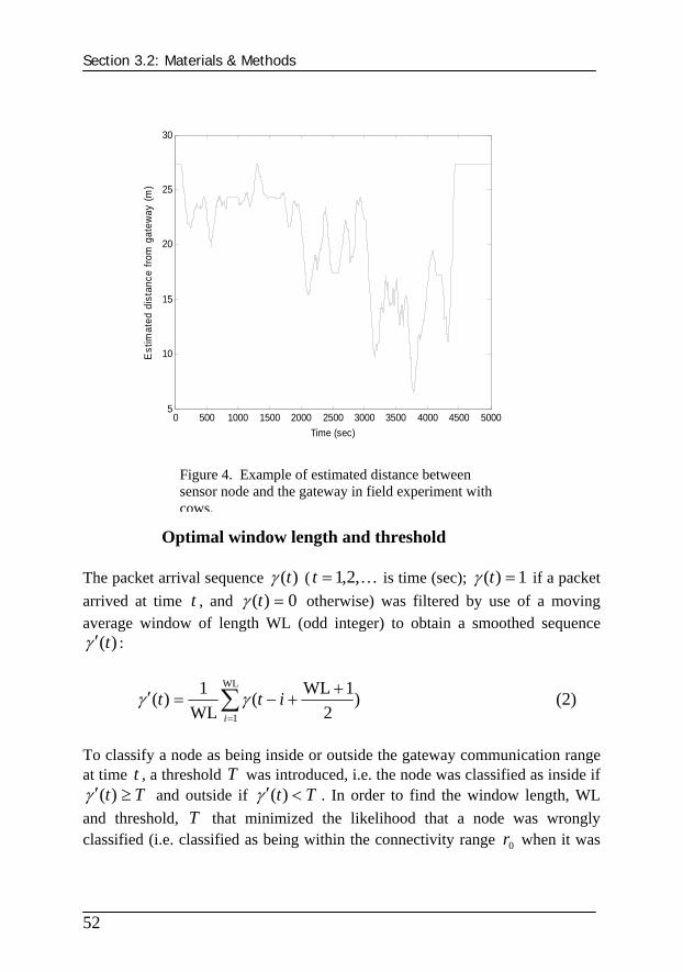
Section 3.2: Materials & Methods

52

Optimal window length and threshold

The packet arrival sequence )(tγ ( K,2,1=t is time (sec); 1)( =tγ if a packet arrived at time t , and 0)( =tγ otherwise) was filtered by use of a moving average window of length WL (odd integer) to obtain a smoothed sequence

)(tγ ′ :

∑=

++−=′

WL

1)

21WL(

WL1)(

iitt γγ (2)

To classify a node as being inside or outside the gateway communication range at time t , a threshold T was introduced, i.e. the node was classified as inside if

Tt ≥′ )(γ and outside if Tt <′ )(γ . In order to find the window length, WL and threshold, T that minimized the likelihood that a node was wrongly classified (i.e. classified as being within the connectivity range 0r when it was

0 500 1000 1500 2000 2500 3000 3500 4000 4500 50005

10

15

20

25

30

Time (sec)

Est

imat

ed d

ista

nce

from

gat

eway

(m)

Figure 4. Example of estimated distance between sensor node and the gateway in field experiment with cows.

Chapter 3

53

not and vice versa) a minimization criterion was defined:

∑= )(min 2

,WLteJ

T (3)

where the classification error )(te was defined as:

⎩⎨⎧ ≤<>≥−

=otherwise0

))(ˆand)('(or))(ˆand)('(if)(')( 00 rtrTtrtrTtTt

teγγγ

(4) In equation (4), )(ˆ tr is the RSS based estimate of the distance between a node and the gateway and 0r (gateway connectivity range) was set to 25 meters based on packet reception rate (example in Figure 5). The selected value of 0r reflects a compromise: on one hand a large value of 0r was desired to make the covered circle as large as possible; on the other hand 0r should not be large to avoid unreliable classification because of low reception rate at high distances from the gateway (Figure 5). Among all the facts which can intensify packet loss rate such as environmental condition, distance, relative height between transceiver and receiver, transmission power, data rate, packet size and the routing protocol; environmental effect and the relative height are mainly the factors that caused high rate packet loss. While the experiment and therefore the calibration process were accomplished in rainy days in the field (outdoor), low reception rate is expected due to high humidity rate where the radio waves can be more easily absorbed by the water and the wet grass. As the curve of packet reception rate versus relative height between sensor nodes and the gateway ascends until a certain relative height and then reaches the steady state, relatively short distance between nodes and the ground and the gateway (40 cm) could be a reason for high packet loss rate.

Pasture time estimation

In order to monitor the pasture time in the strip of new grass, the field was extended by moving a section of the fence. As it is shown in Figure 6, the rectangular extended area, Δ (which is the strip of new grass) was not entirely covered by the gateway connectivity area which implies that time spent in that

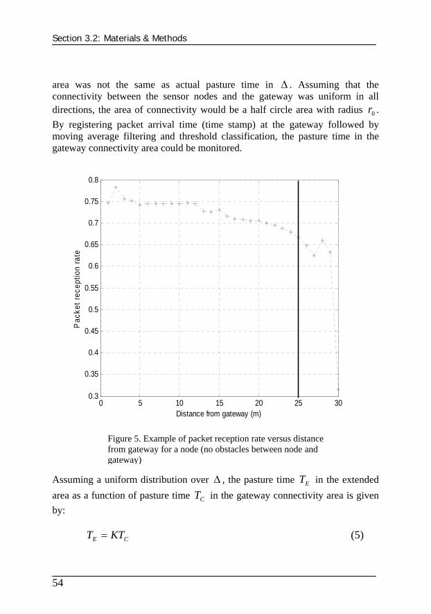
Section 3.2: Materials & Methods

54

area was not the same as actual pasture time in Δ . Assuming that the connectivity between the sensor nodes and the gateway was uniform in all directions, the area of connectivity would be a half circle area with radius 0r . By registering packet arrival time (time stamp) at the gateway followed by moving average filtering and threshold classification, the pasture time in the gateway connectivity area could be monitored.

Assuming a uniform distribution over Δ , the pasture time ET in the extended area as a function of pasture time CT in the gateway connectivity area is given by:

CE KTT = (5)

0 5 10 15 20 25 300.3

0.35

0.4

0.45

0.5

0.55

0.6

0.65

0.7

0.75

0.8

Distance from gateway (m)

Pac

ket r

ecep

tion

rate

Figure 5. Example of packet reception rate versus distance from gateway for a node (no obstacles between node and gateway)

Chapter 3

55

where constant K is the ratio of the extended area (Δ ) to the gateway connectivity area ( 2

0rπ /2). Since the constant K depended only on fixed geometrical quantities, it was the same constant for all individuals in the herd.

Testing the hypothesis that monitored cows could represent the entire herd

To estimate pasture time for the entire herd of cows based on data from the monitored subset of the herd (23%), it was assumed that the monitored cows could represent the whole herd. The validity of this assumption was examined by statistical tests that involved two random variables: 1D , the number of monitored cows in the extended area, and 2D , the total number of cows in that area. Both of these variables were sampled each minute over three hours by manual observation. First, it was tested if the distributions of 1D and 2D could be approximated by normal distributions. Then it was tested if the ratio between the means of 2D and 1D was equal to the ratio k between the total number of

cows and the number of monitored cows ( 3.4730 ==k ). If the result of this

Section 3.2: Materials & Methods

56

test was positive, it would indicate that the monitored cows could represent all cows in the herd (with respect to pasture time in the extended area).

Test of the normal approximation

Pearson's chi-square test ( 2χ ) is one of a variety of chi-square statistical procedures whose results are evaluated by reference to the chi-square distribution (Chernoff and Lehmann, 1954). Pearson's chi-square is used to assess tests of goodness of fit which establishes whether or not an observed distribution differs from a theoretical distribution. Pearson chi-square tests were applied to the samples of 1D and 2D to evaluate whether the variables were normally distributed.

Testing if the monitored cows was a representative sample of the herd

In order to evaluate if the monitored subset of the herd could represent the whole herd, the following null hypothesis 0H and alternative hypothesis 1H were set up:

121

120

::

μμμμ

kHkH

≠=

s.t. 22

21 σσ ≠ (6)

where 1μ and 2μ are the theoretical and unknown mean values of 1D and 2D respectively. 1σ and 2σ are the theoretical and unknown standard deviations of

1D and 2D and k is a constant representing the ratio of the number of monitored cows to the total number of cows. In order to define significance level (α ), the probability function has been introduced: ) trueisreject( 00 HHp=α (7) To reject the null hypothesis, modifications to the standard test were required to incorporate the ratio k . A modified version of the two-sample t test was applied. The result is a criterion for rejection, vtt ,210 α−> where vt ,21 α− is the

21 α− quantile in the Student’s t-distribution with v degrees of freedom. The

Chapter 3

57

t-statistics 0t and the degrees of freedom v are defined as:

1

21

2

2

22

120

nsk

ns

ykyt

+

−= (8)

11 1

2

1

21

2

2

2

2

22

2

1

21

2

2

22

−

⎟⎠⎞

⎜⎝⎛

+−

⎟⎠⎞

⎜⎝⎛

⎟⎟⎠

⎞⎜⎜⎝

⎛+

=

n

nsk

n

ns

nsk

ns

v (9)

In equation (8) and (9), 1y and 2y are the sample means of 1D and 2D , respectively while 1s and 2s are the sample standard deviations of 1D and

2D . The sample sizes for 1D and 2D are 1n and 2n respectively.

III. EXPERIMENTAL SETUP & RESULTS

Experimental setup The case study in the presented experiment was a group of dairy cows. The experiment was carried out during 6 days with 30 cows 6 hours per day on average. Data from three days of the experiment were used for estimation of the optimal window length and threshold of the filter used for the packet arrival sequence. The packet arrival sequence from the remaining three days were filtered and applied for estimation of pasture time in the strip of new grass. During the calibration process, the nodes were placed at fixed distances (1 to 30 meters far from the gateway) for 5 minutes at each distance. The sampling time was set to 1 second and it was expected to receive 300 samples per distance while the real number of packets received at each distance is presented by packet reception rate in Figure 5. The experimental data in Figure 3 represents the mean value of the readings taken at each distance. Seven out of 30 cows were equipped with wireless nodes around the neck. The node on the collar as well as collar itself was fixed very well to prohibit any

Section 3.3: Experimental setup & Results

58

slide to right or left side. The antenna pointed the sky in order to have better communication between nodes and the gateway. The antenna was ½ wave dipole antenna, with an MMCX connector. The gateway was installed 1.2 meters above the ground in a location as indicated in Figure 1. The shape of the extended area was rectangular and the area was 60 meters by 40 meters while the shape of the gateway connectivity area was a half circle with a radius of 25 meters. Each day, a new extended area covered by new grass was provided for the cows. Manual registrations of absolute time of day when each of the 30 cows was in the extended area and the connectivity area were carried out 3 hours per day during 3 days. Furthermore, the number of cows roaming in the extended area was registered manually with a sampling interval of one minute during different grazing periods (e.g. first grazing period starts when the animal enters the field and second grazing period starts after first lying down period). Results and discussion

Pasture time monitoring

Minimizing the cost function in equation (3) resulted in an optimal window length and threshold of 155 seconds and 0.388, respectively. The result of applying the moving average window with the optimal window length and the threshold to the packet delivery performance (Figure 2) is presented by Figure 7. While the delivery rate in the packet delivery performance was 68.8% (31.2% packet loss), applying the optimal window improved the results of packet delivery to 92%. Moving average filtering and subsequent classification of presence inside or outside the connectivity area were compared to manual registrations and resulted in errors as exemplified in Figure 8 and Figure 9 for two different nodes. Values of 0 and 1 indicate correct and incorrect classification, respectively. The percentages of successful classification for the entire experiment are presented in Table 1. In order to estimate the total pasture time length for each of the monitored cows in the extended area using estimated total pasture time length in the gateway connectivity area, equation (5) was applied with 44.2=K as the extended area was 2m2400 and gateway connectivity area was 2m74.981 . Statistical analysis of the cows’ GPS positions confirmed that they were uniformly distributed over the extended area.

Chapter 3

59

Table 2 shows the estimated pasture time as percentage of true pasture time for all the monitored cows during the experiment. As it can be concluded from Table 2, the estimated total pasture time using equation (5) was always an underestimation of the real total pasture time. One reason for this could be that the packet loss rate was generally higher in this experiment than it was in the experiment used for finding the optimal window length and classification threshold. Apart from the proposed moving average window, a potential solution for the problem of packet loss could be as introduced by Guo et al., (2006) in which an onboard flash memory was used in their designed nodes to store considerable amounts of data. Stored packets would then be sent to the gateway as soon as nodes could communicate to the gateway. However, this solution to the problem of packet loss would require extra hardware facilities and causes delay in classifying the presence or absence in the communication range of the gateway, this relatively short delay will not have a critical influence on the performance of the monitoring system.

0 100 200 300 400 500 600 700 800 9000.3

0.4

0.5

0.6

0.7

0.8

0.9

1

Time (sec)

Filte

red

pack

et d

eliv

ery

perfo

rman

ce

Figure 7. Filtered packet delivery performance by the optimal moving average window. The threshold (0.388) is presented by the horizontal line.

Section 3.3: Experimental setup & Results

60

0 2000 4000 6000 8000 10000 12000 140000

0.2

0.4

0.6

0.8

1

1.2

Time (Sec)

Pre

senc

e E

rror i

n C

onne

ctiv

ity A

rea

Figure 8. Classification error for one of the nodes, example 1.

0 2000 4000 6000 8000 10000 12000 140000

0.2

0.4

0.6

0.8

1

1.2

Time (Sec)

Pre

senc

e E

rror i

n C

onne

ctiv

ity A

rea

Figure 9. Classification error for one of the nodes, example 2.

Chapter 3

61

Section 3.4: Conclusions

62

Normality test for number of cows in the extended area

In order to evaluate whether the total number of cows ( 2D ) in the extended area was normally distributed using Pearson chi-square test, contingency tables were constructed for data from all days. As an example, Table 3 presents the contingency tables for two different datasets containing of total number of cows ( )1(

2D and )2(2D ) in two different grazing periods from the first day. It was

concluded from the Pearson chi-square test of goodness of fit with 2 degrees of freedom that 2D was normally distributed (hypothesis accepted at a significance level of 0.2). As presented in Table 3, the estimated mean value of )2(

2D (total number of cows in the extended area during second grazing period) is smaller while the estimated variance is larger compared to the estimated mean value and variance of )1(

2D (total number of cows in the extended area during first grazing period) with grass offer reduction. Pearson chi-square test of goodness of fit was also applied to 1D and the results demonstrated that the distribution of 1D during first an second grazing period ( )1(

1D and )2(1D ) was Gaussian (hypothesis accepted at a significance level of

0.2) and the estimated mean value of )1(1D and )2(

1D was 2.6 and 2.4 respectively.

Testing the hypothesis that monitored cows could represent the entire herd

The results of testing the null hypothesis in equation (6) are shown in Table 4. The significance level is chosen equal to 0.2 (Montgomery, 1996). Based on the results of the last row in Table 4, it is concluded that the introduced null hypothesis can not be rejected.

IV. CONCLUSION The problem of online monitoring of cows’ presence and pasture time in an extended area in the field with new grass has been addressed and solved by using wireless sensor networks. The total pasture time in the extended area was estimated by measuring the pasture time in the gateway connectivity area where

Chapter 3

63

the sensor nodes could communicate directly to the gateway. However, as the measured time in the connectivity area underestimated the total pasture time in the extended area, an area based correction factor was applied and the results showed 79.9% success rate (21.1% error) on average. As only 23% of the animals were equipped to be monitored by sensor nodes, investigations to evaluate whether the monitored animals could represent the whole herd were carried out. Pearson chi-square test of goodness of fit has been successfully applied to the datasets containing the number of cows roaming in the extended area and the number of cows carrying sensor nodes in the extended area. The results of statistical analysis indicated that the datasets were normally distributed.

Section 3.4: Conclusions

64

The hypothesis was that cows with and without sensor nodes would spend the same relative amount of time in the extended area. This hypothesis was confirmed by a modified two sample t test for the expected relation between the mean number of cows with sensor nodes in the extended area and the mean number of cows totally in the extended area. Applying a moving average window with optimal window length and optimal threshold could successfully compensate for packet loss between sensor nodes and gateway and thereby improve the result of classification as being within or outside communication range of the gateway.

Chapter 3

65

REFERENCE

Bishop-Hurley, G. J., Swain, D. L., Anderson, D. M., Sikka, P., Crossman, C., Corke, P., 2007. Virtual fencing applications: Implementing and testing an automated cattle control system. Journal of Computers and Electronics in Agriculture, Vol. 56, Issue 1, pp.14-22.

Butler, Z., Corke, P., Peterson, R., Rus, D., 2004. Networked Cows: Virtual Fences for Controlling Cows. In Proceedings of ICRA. IEEE Conference on Robotics and Automation, New Orleans, LA. Vol. 5, pp.4429 – 4436.

Chernoff, H., Lehmann, E.L., 1954. The use of maximum likelihood estimation in chi-square test of goodness o fit. The annals of mathematical statistics.

Guo, Y., Corke, P., Poulton, G., Wark, T., Bishop-Hurley G., Swain, D. 2006. Animal behavior understanding using wireless sensor networks. In proceedings of the 1st IEEE international workshop on practical issues in building sensor network applications (SenseApp 2006); Tampa, Fl, IEEE, pp. 608-614.

Kotanen, A., Hannikainen, M., Leppakoski, H., Hamalainen, T.D. 2003. Experiment on local positioning with Bluetooth. Information Technology: Coding and Computing [Computers and Communications], 2003. Proceedings. ITCC 2003. International Conference, pp. 297 – 303.

Lewis, F. L., 2004. Wireless sensor networks. Smart environments: Technologies, Protocols and Applications. ed. D.J. Cook and S.K. Das, John Wiley, New York. ISBN: 978-0-471-54448-7

Montgomery, D., C. 1996. Design and analysis of experiments. John Wiley & Sons, United states of America. Fourth edition.

Munksgaard, L., Jensen, M.B., Herskin, M.S., Levendahl, P., 2005. The need for lying time in high producing dairy cows. In proceedings of the 39th International Congress of the ISAE, Kanagawa, Japan, pp. 38-42.

Nadimi, E. S., Bak, T., Izadi-Zamanabadi, R. 2006. Monitoring animals and herd behavior parameters using a wireless sensor network.

References

66

Proceedings of XVI CIGR world congress. Book of abstracts, pp. 415-416.

Nadimi, E. S., Søgaard, H. T., Oudshoorn, F. W., Blanes-Vidal, V., Bak, T. 2007. Monitoring Cow Behavior Parameters based on Received Signal Strength using Wireless Sensor Networks. In proceedings of 3rd European Conference on Precision Livestock Farming (ECPLF). Edited by: S. Cox. pp.95-103. ISBN: 978-90-8686-023-4

Ng, M. L., Leong, K. S., Hall, D. M., Cole, P. H., 2005. A simple passive UHF RFID tag for livestock identification. Proceedings of IEEE international symposium on microwave, antenna, propagation and EMC technologies for wireless communication. pp. 67-70.

Oudshoorn, F. W., Nadimi, E. S., 2007. Intelligent grazing management using wireless sensor networks. In proceedings of 3rd European Conference on Precision Livestock Farming (ECPLF). Edited by: S. Cox. pp.111-116. ISBN: 978-90-8686-023-4

Oudshoorn, F. W., Kristensen, T., Nadimi, E. S., 2007. Dairy cow defecation and urination frequency and spatial distribution related to time limited grazing, accepted in the journal of livestock production sciences. Livestock Science (2007), doi:10.1016/j.livsci.2007.02.021

Schwager, M., Anderson, D. M., Butler, Z., Rus, D., 2007. Robust classification of animal tracking data. Journal of Computers and Electronics in Agriculture, Vol. 56, Issue 1, pp.46-59.

Sinopoli, B., Schenato, L., Franceschetti, M., Poolla, K., Jordan, M. I., Sastry, S.S., 2004. Kalman filtering with intermittent observation. IEEE transaction on automatic control, Vol. 9, pp. 1453-1464.

Szewczyk, R., Osterweil, E., Polastre, J., Hamilton, M, Mainwaring, A., Estrin, D., 2004. Habitat monitoring with sensor networks. Journal of Communications of the ACM, Vol.47, issue 6, pp.34-40.

Torjusen, H., Lieblein, G., Wandel, M., Francis, C., A., 2001. Food system orientation and quality perception among consumers and producers of organic food in Hedmark County, Norway. Journal of food quality and preference, Vol. 12, issue 3, pp. 207-216.

Wang, N., Zhang, N., Wang, M., 2006. Wireless sensors in agriculture and food industry-recent development and future perspective.

Chapter 3

67

Journal of computers and electronics in agriculture. Vol. 50, Issue 1, January 2006, pp. 1-14.

White, S. L., Sheffield, R. E., Washburn, S.P., King, L. D., Green, J. T., 2001. Spatial and Time Distribution of Dairy Cattle Excreta in an Intensive Pasture System, journal of Environmental Quality. Vol. 30, pp. 2180-2187.

Wilson, S.C., Dobos, R.C., Fell, L.R., 2005. Spectral analysis of feeding behavior of cattle kept under different feedlot conditions”. Journal of Applied Animal Welfare science. Vol. 8, Issue 1, pp. 13-24.

CHAPTER 4 ZigBee Based Wireless Sensor Networks for Classifying the Behavior of a Herd of Animals Using Classification Trees

Section 4.1: Introduction

70

ZigBee Based Wireless Sensor Networks for Classifying the Behavior of a Herd of Animals Using Classification Trees

1,2E. S. Nadimi, 1H. T. Søgaard, 2T. Bak

1Research Center Bygholm, Department of Agricultural Engineering, Aarhus University, Denmark 2Department of Electronic Systems, Automatic and Control, Aalborg University, Denmark

Email: esmaeil.nadimi@agrsci.dk; henningt.sogaard@agrsci.dk; tba@es.aau.dk Abstract An in-depth study of wireless sensor networks applied to monitoring of animal behavior in the field is provided. Herd motion data such as pitch angle of the neck and the movement velocity were respectively monitored by an MTS310 sensor board equipped with a 2-axis accelerometer and received signal strength indicator functionality in a single hop wireless sensor network. Pitch angle measurements as well as velocity estimates were transmitted through a wireless sensor network based on ZigBee communication protocol. After data filtering, the pitch angle measurements together with velocity estimates were used to classify the animal behavior into two classes as active and inactive. Considering all the advantages and drawbacks of classification trees compared to neural network and fuzzy logic classifiers, a general classification tree was preferred. The classification tree was constructed based on the measurements of pitch angle of the neck and movement velocity of some animals in the herd and was used to predict the behavior of other animals in the herd. The results showed that there was a large improvement in the classification accuracy if both pitch angle of the neck and velocity were employed as predictors in comparison to just pitch angle or just velocity employed as the single predictor. The classification results proved the possibility of determining a general decision rule which can classify the behavior of each individual in a herd of animals. The results have been confirmed by manual registration and by GPS measurements. Keywords: Received signal strength; Kalman Filter; Kaiser window; ZigBee; Wireless sensor network; Classification tree; Behavior monitoring.

I. Introduction Animal behavior monitoring represents a class of wireless sensor network applications with enormous potential benefits for practical farming. In this sense, the knowledge of the herd behavior phases (activity, inactivity) can be

Chapter 4

71

monitored by measuring relevant behavior parameters. Such behavior classification is potentially useful as management tools in grazing and production optimization. Furthermore, the behavioral monitoring would allow us to establish a better understanding of animal behavior, detect individuals with potential health problems, and generally optimize the grazing process.In order to monitor herd behavior, data relevant to the behavior should be measured, aggregated, processed and finally sent through a network to infrastructure facilities. In animal science applications, the natural mobility of the herd makes wireless sensor networks the perfect candidate for such monitoring of animal behavior parameters. Furthermore, wireless sensor networks represent a significant advance over traditional invasive methods of monitoring. The integration of local processing and storage allows sensor nodes to perform complex filtering and triggering functions, as well as to apply application-specific or sensor-specific data compression algorithms. Low-power radios with well-designed protocol stacks allow generalized communications among network nodes, rather than point-to-point telemetry. The computing and networking capabilities allow sensor networks to be reprogrammed or retasked after deployment in the field. Therefore, monitoring animal behavior parameters using wireless sensor networks leads to a flexible and robust monitoring system capable of remotely registering the behavior parameters which are of interest. A herd of animals differs in many ways from man-made systems of mobile robots because the behavior of each individual is governed by unpredictable natural instincts and the environment in which it is placed (e.g. motion patterns influenced by food sources and water). Therefore, different aspects of animal behavior by monitoring variety of behavioral parameters have been studied by different researchers. As instance, the position of animals in the field were tracked and monitored by White et al., (2001); Butler et al., (2004); Zhang et al., (2004); Schwager et al., 2007 and Wark et al., (2007) while Oudshoorn et al., (2006) made their investigation based on the positions and the velocities of the movements in the field. Different behavior phases of dairy cows such as standing and lying down when they were in the barn are evaluated by Munksgaard et al., (2005) and Wilson et al., (2005). However, none of these references address an online monitoring system based on wireless sensor networks that classifies the behavior of the animals when they are in the field. The behavioral parameters can be measured using different types of sensors and consequently different strategies. GPS is the most popular system employed in outdoor applications to register position (Butler et al., 2004; Oudshoorn et al., 2006 and Schwager et al., 2007) but high energy consumption is one of the main drawbacks of such a localization method. Furthermore, satellite connection loss in the areas of the field covered by trees has been reported

Section 4.2: Problem statement and background

72

frequently in the research done by Oudshoorn et al., (2006). This makes GPS less practical in terms of long-term studies and less reliable for animal monitoring in some specific environments. Using an accelerometer attached to the leg of animal together with an offline data logger inside barn was another approach used in the experiments carried out by Munksgaard et al., (2005). They classified cow behavior into two phases as moving or stationary, while Umstatter et al., (2006) used an offline pitch-roll sensor around the neck. Sallvik & Oostra (2005) used video processing combined with RFSU (radio frequency synchronization unit). In the present paper, a wireless sensor network was established in which ZigBee was implemented as the wireless communication protocol. Each node in the network was equipped with an accelerometer in order to measure the pitch angle of the neck. The nodes were programmed to measure received signal strength (RSS) allowing the distance between wireless sensors and a gateway to be estimated. Based on successive distance estimates, the velocity could be estimated. In order to fuse the measured behavior parameters (i.e. pitch angle of the neck and the movement velocity) and consequently to be able to classify the animal behavior into classes as active or inactive, different classification methods such as decision trees, fuzzy logic and neural networks have been introduced in the literature. Comparing advantages and drawbacks of decision trees compared to Fuzzy logic and neural network classifiers made them the best candidate in terms of simplicity and accuracy to evaluate the herd behavior and they have hence been employed as the classification method. The objectives of this paper were to classify the behavior of a herd of animals into two classes as active and inactive using the pitch angle measurements of the neck of the animal together with the movement velocity estimates in a wireless sensor network. Yet another objective was to solve a specific problem regarding packet loss using data post processing. The remainder of this paper is organized as follows. Problem statement and a short review on wireless sensor networks are presented in section 2. Section 3 describes materials and methods that have been used to classify the behavior phases. Section 4 describes the results achieved by this research and finally, the conclusions are presented.

II. Problem statement & background Problem statement In this paper, the problem of online robust classification of the animal behavior using a wireless sensor network has been addressed. The main deficiencies

Chapter 4

73

reported in the research done by Umstatter et al., (2006), Nadimi et al., (2007) and Schwager et al., (2007) were:

• Local, non-representative peaks may occur because only the minimum value of the pitch angle of the neck was recorded during each sampling interval. (Umstatter et al., 2006)

• Disability of online measuring. (Umstatter et al., 2006) • Simple-non robust classification method. (Nadimi et al., 2007) • High energy consumption method to estimate the behavior of animals

(Schwager et al., 2007) The first two problems can make the classification results unreliable. Therefore they are addressed in this paper and solved by using a Kalman filter and weighted moving average window together with velocity estimation using RSS measurements. As the simple threshold method (two dimensions classification tree) used in the research carried out by Nadimi et al., (2007) made the classification non robust and in order to reduce the risk of an improper classification, decision trees, fuzzy logic and neural network classification methods have been applied. Consequently, decision tree due to its simplicity for training, accuracy and applicability was chosen as the most suitable classification approach. To employ a low-cost and low-power monitoring system, wireless sensor networks have been implemented in the present research, therefore the deficiency (high energy consumption) introduced in the research carried out by Schwager et al., (2007 ) is addressed. In order to address the problem of packet loss which occasionally occurs in monitoring moving nodes in outdoor environments using wireless sensor networks, an efficient solution is proposed by predicting the lost states using a Kalman filter which is presented in this paper. Background Location systems in outdoor environments have been a research interest in the last years. The methods for locating a target in a geographical area based on received signal can be classified in three different groups of which the latter was studied in this paper.

• Time of arrivals (TOA) algorithms These algorithms measure the time a signal needs to travel from a beacon to the target node. As distances in pasture fields are not very big, the relative resolution acquired using radio signals is very poor. However, other kinds of signals, such as sound with a smaller wavelength are easier to track (Harter et

Section 4.3: Materials and methods

74

al., 1999; Priyantha et al., 2000; Ward et al., 1997), so the radio interface may be used to synchronize the network nodes, and the sound signal to measure distances. The precision of these methods is very good, but it requires some additional hardware, in order to produce and detect the sound signal.

• Angle of arrivals (AOA) algorithms These algorithms measure the direction, the arriving signal comes from. Using the laws of sine and cosine, the position of the target node can be calculated (Arias et al., 2004). The hardware needed may be quite complex, as it requires either a mechanical system that moves the antenna or an antenna array, whose radiation pattern can be altered electronically.

• Received signal strength (RSS) algorithms In order to get an accurate estimate of the distance between nodes based on TOA and AOA algorithms, additional localization hardware in terms of antennas or high precision clock synchronization is required. However, RSS algorithms are based on the fact that a radio signal attenuates with increasing distance from the emitter. If the emitted power is known, measuring the incoming power at the receiver, the distance between the transceiver and receiver can be estimated. Nevertheless, the medium exerts a substantial influence on the arriving signal power; obstacles attenuate the signal and produce reflections. Other signals or even the reflections of the signal of interest may interfere with the emitted signal, which alters the signal’s power (Arias et al; 2004). In order to estimate the distance from RSS values, range measurements should be done, i.e. estimating the distance between two nodes, given the signal strength received by one node from the other. Signal strength measurements are usually prone to inaccuracies and errors and, hence, calibration of such measurements is inevitable before using them for localization. For this algorithm to work, extensive preliminary field measurements and calibrations were carried out as discussed in the following.

III. Materials and methods Materials MPR2400 Micaz sensor motes from Crossbow were used for the experiments in this paper. They have a Chipcon CC2420 radio, which uses a 2.4 GHz IEEE 802.15.4/ZigBee RF transceiver with MAC support and provides a received signal strength indicator (RSSI) output that is sampled by a 10-bit ADC. An MTS310 sensor board equipped with a 2-axis accelerometer and a temperature

Chapter 4.

75

sensor was used to measure the pitch angle of the neck of a cow. The temperature sensor was used to calibrate the accelerometer readings as the digital output of the accelerometer (duty cycle) can be varied by temperature drifts. Consequently, to use the accelerometer as a dual-axis tilt sensor to measure the pitch angle of the neck of the cow, the raw accelerometer ADC readings were converted to acceleration measurements (Analog device, 2007). TinyOS operating system was running on the motes (Gay et al., 2007). The RSS data and the accelerometer readings together with the temperature measurements were encapsulated in the same packet. This designed packet structure solve the problem reported by Nielsen et al., (2005) in which two different packet structures were used to disseminate the data of RSS and acceleration. If each sensor disseminates two kinds of packets, for instance one for RSS and the other one for acceleration, losing one of them make the other packet useless. The selected sampling rate for the packet dissemination was 1 Hz (Nadimi et al., 2006). Multiple sensor nodes sent sensor readings to a base station or aggregation point in the network (gateway) using many to one routing protocol. The CC2420 radio supports up to 255 different transmission power levels and allows for a programmable transmission frequency. In order to minimize the number of variables in the experiment, the RF transmission frequency and the transition power were respectively fixed at a single frequency band (2.48 GHz) and at the maximum transmission power (1 mW). The case study in this experiment was a group of dairy cows. The experiment was carried out during 3 days with 4 cows 6 hours per day as an average. Each cow was equipped with a wireless node and a GPS as a reference around the neck (Figure 1). During the calibration process, the nodes were placed at fixed distances (1–30m far from the gateway) for 5 minute at each distance. The sampling time was set to 1 second and it was expected to receive 300 samples per distance. As without any energy budgeting, MPR2400 Micaz nodes operating at 100% duty cycle can approximately operate for seven days (Polastre, 2003), normal AA batteries with a conservative estimate of 2200 mAh total capacity was utilized which provided enough power for each sensor node during the whole experiment (3 days). The shape of the field was rectangular ( 4080× meters). Each day, a new field with new grass was provided for the cows. The gateway was installed in the middle of one of the longest sides. Manual registration of the behavior was carried out as well.

Section 4.3: Materials and methods

76

Methods RSS and acceleration measurements filtering When data travel along unreliable communication channels in a large, wireless sensor network, the effect of communication delays and loss of information cannot be neglected. This problem is addressed here using separate discrete Kalman filters for RSS and acceleration observation where the arrival of observation packets is modeled as a random process. The statistical convergence properties of the state error covariance have been studied, showing the existence of a critical value for the arrival probability of the observations, beyond which a transition to an unbounded state error covariance occurs. Due to high rate energy absorption in outdoor applications, packets either arrive or are lost within a sampling period following a Bernoulli process with parameter

10 ≤≤ λ (packet arrival probability). A Kalman Filter, however, still provides estimates in case of intermittent observations (Sinopoli et al., 2004). With these assumptions, the Kalman filter equations for scalar states and measurements are as follows:

• Time update equations:

Node

GPS

Figure 1. Wireless node and GPS around the neck

Y

X

Chapter 4.

77

kkk xx ˆˆ 1 ϕ=−+ (1)

kkkkk QPP +=−+

T1 ϕϕ (2)

• Observation updates equations −−= kkkkk PHKP )1( γ (3)

)ˆ(ˆˆ −− −+= kkkkkkk xHzKxx γ (4)

1TT )( −−− += kkkkkkk RHPHHPK (5) where K,2,1,0=k is the time instant, −

kx̂ and kx̂ are a priori and posteriori

state estimate which a state could either be RSS or acceleration. −kP and kP are

a priori and posteriori estimate of error variance, and kK is the Kalman gain.

kQ is the process noise covariance, kR is the measurement noise covariance.

kγ is the arrival sequence which is common for the RSS filter and the acceleration filter and is modeled by a Bernoulli process (1 if arrived; 0 if lost). The underlying process (pitch angle of the neck and the movement velocity) has been assumed as a discrete time Wiener process described by equations (6) and (7) in the state space form. kkkk wxx +=+ ϕ1 (6)

kkkk vxHz += (7) where, kx is the true (unknown) state, kz is the RSS measurements or acceleration measurements if the packet arrives, ),0( kk QNw ∈ is the process noise and ),0( kk RNv ∈ is the measurement noise ( kw and kv are independent). kH and kϕ are set to 1 independently of time ( k ). To estimate the states, separate scalar filters for RSS and acceleration has been employed. As the Kalman filter is designed to handle intermittent observations, it will estimate the states not observed due to the packet loss and thereby reduce the effect of measurement noise. The existence of a critical value cλ for the arrival probability of the observation update has been shown by Sinopoli et al., (2004), such that for cλλ > , the mean state covariance [ ]kPΕ is bounded for all initial conditions and for

Section 4.3: Materials and methods

78

cλλ ≤ the mean state covariance diverges for some initial condition. A lower

bound λ , and upper bound λ can be found for the critical probability cλ , i.e;

λλλ ≤≤ c . The lower bound can be expressed in closed form while the upper bound is the solution of a linear matrix inequality (LMI). In some special cases when kH is invertible or kϕ has a single unstable eigenvalue, the two bounds coincide, giving a tight estimate. Since kH is set to 1, the critical arrival probability can be expressed as (Sinopoli et al., 2004):

211 pc −=λ ))(eigmax( kp ϕ= (8)

As the average value of λ was 0.7 in the present study and 0=cλ for a discrete time Wiener process, the inequality cλλ > was fulfilled. During the grazing period, the head moves upwards with certain intervals and thereby make the pitch angle readings close to zero during very short periods of time (Umstatter et al., 2006). To avoid classifying these events as parts of an inactivity phase, the Kalman filtered data were further filtered using a weighted moving average window. In order to select an appropriate window, the properties of different common windows such as Rectangular, Bartlett, Hanning, Hamming, Blackman and Kaiser Window have been considered. The two main criteria to measure the performance of different windows are (Ashan, 2003):

• Smearing reduction or spectral resolution improvement which can be achieved by reduction of the main lobe width in frequency domain

• Leakage reduction or amplitude resolution improvement which can be achieved by side lobe reduction

The first property is the ability of the filter to separate signals whose frequencies are nearly the same while the second property is the capability of separating unequal amplitudes in order to prevent that low amplitude peak drowns in the leakage of the higher amplitude peak. To fulfill the criteria, narrow main lobe width and low side lobe amplitude is required. While these two conditions can not be met simultaneously, the trade off between the main lobe width and side lobes’ amplitudes can be quantified by a Kaiser window represented by (Oppenheim et al., 1999):

Chapter 4.

79

⎪⎪⎩

⎪⎪⎨

⎧

≤≤−−

=

otherwise0

0if)(

))12(1(

0

20

NnI

NnI

Wn πα

πα (9)

where )(0 ⋅I is the zeroth order modified Bessel function of the first kind. The real parameter α which determines the shape of the window is set to 0.5 and the integer N gives the length of the window ( 1+N points). The window length was chosen less than the length of typical inactive periods to be sure that these periods would be detected ( 1000=N , i.e. 0.278 h). Acceleration measurements analysis In the active period, the animals are grazing or looking for grass so their necks are down and the movement velocities are nonzero. In the inactive phase, the necks are almost horizontal and the movement velocities are zero. Therefore measuring the pitch angle of the neck together with the movement velocity is chosen as the basis for the behavior classification. To measure the pitch angle of the neck, the MTS310 sensor board was installed around the neck. In order to convert the raw accelerometer ADC readings to the acceleration measurements, the values of bias and sensitivity of each sensor by orienting the accelerometer axis towards the gravity axis (+1g and -1g) have been calculated. Furthermore, the relationship between acceleration and pitch angle is based upon inverse sine and cosine functions using the fact that the accelerometer measures the components of the gravity acceleration parallel to the local coordinate system (X-Y plane) of MTS310 sensor board (Figure 1). Figure 2 shows an example of the graph of pitch angle after using a moving window placed symmetrically around the time instant of interest. RSS measurement analysis In order to get an accurate estimate of the distance between nodes based on received signal strength, extensive preliminary field measurements and calibrations were carried out. Figure 3 shows the graph of signal strength versus distance for one of the nodes for a typical outdoor setup in field. The experimental data in Figure 3 represents the mean value of the readings taken at each distance. The received power level can be converted to a distance estimate by using a radio wave propagation model (Kotanen et al., 2003). A simple log-distance model was used:

Section 4.3: Materials and methods

80

)4log(20)log(20log10 πλ −+++−= WLRxTxRxTxe GGPPdn (10) where [ ]dBmTxP and [ ]dBmRxP are the transmitted ( dBm0 ) and received power levels (RSS), respectively. [ ]dBiTxG and [ ]dBiRxG are antenna gains of the transmitter and the receiver. [ ]mWLλ is the wavelength, and [ ]md is the distance between transmitter and receiver. The exponent en is assumed to attain a value of 2 for outdoor environments (Kotanen et al., 2003; Nadimi et al., 2007). Calculating the antenna gain in equation (10) is not a simple procedure so a propagation model has been fitted to experimental data. In this model, the last four terms in equation (10) were combined into one constant C (see equation 11) which was estimated by minimizing the sum of squared differences between the experimental RSS and the modeled RSS.

CPPd RxTx +−=log20 (11) As all the nodes have different characteristics such as different antenna gains or

X

Figure 2. Pitch angle of the neck passed through Kalman – Kaiser Filter

0 1 2 3 4 5 6-70

-60

-50

-40

-30

-20

-10

Time, Hour

Pitc

h A

ngle

, Deg

ree

Chapter 4.

81

different radios, the graph of received signal strength versus distance (Figure 3) is not the same for all the nodes. Therefore, the optimal constant C in Equation (11) is different from one node to another one (the range varied between −60 dBm to −55 dBm). In the present research, the constant C calculated for one of the nodes (−56 dBm) was selected as the optimal constant representing antenna gain and wavelength effect for all the nodes. This strategy tends to descend precision of the results of each individual node (curve fit and estimated distance between nodes and gateway) and consequently the whole system. However, that is the practical solution to implement a similar monitoring system to a large herd of animals with a large number of nodes as it will be time and energy consuming process to estimate the optimal constant C for all the nodes. Using equation (11), distance kd between the cow node and the gateway could be estimated for each time instant k , and furthermore the change in distance

0 5 10 15 20 25-90

-85

-80

-75

-70

-65

-60

Distance (m)

Sig

nal s

treng

th (d

Bm

)

Figure 3. RSS versus distance for fitted optimal propagation model and experimental data. Black curve: propagation model, Blue curve: experimental data. Arrows as indicator of error bar (standard deviation) at each point.

Section 4.3: Materials and methods

82

during each sampling interval could be estimated as 1−−= kkk ddD . This distance change was taken as a rough estimate of the distances walked by the cow during the sampling interval. An example of estimated distances walked per sampling interval (velocity) versus time has been shown in Figure 4. A comparison between estimated and true distance walked over one sampling interval (displacement) is illustrated in Figure 5. Based on the methodology used in this research to estimate the velocity using RSS, if an animal walks in a circle around the gateway, the velocity will be estimated as zero. However attention needs to be drawn to the fact that this case can rarely happen, as animal behavior studies have demonstrated that cows use to walk straight forward (Oudshoorn et al. 2007). To prove the visual observation that cows rarely move on a circle, the position of cows in the field was registered by GPS and was sampled every 60 seconds (Figure 6). Based on GPS registrations and the equations of half circles (see Figure 6), it was demonstrated that three consecutive locations were not on a same circle. The mentioned drawback of the method would only become relevant in a large field where the half circles far from the gateway turn to straight lines. In this experiment the size of the field was chosen as 8040× meters and the radius of the largest half circle was 40 meters. In order to verify the estimated distance using received signal strength, a GPS (Figure 1) was employed to measure the position and the distance of wireless nodes from the gateway. Figure 7 (upper graph) shows the measured distance by GPS between one of the nodes and the gateway versus the distance estimated by the RSS approach. Furthermore, Figure 7 (lower graph) presents the distance of a node from gateway measured by GPS and estimated by RSS measurements versus time. The distance between the nodes and the gateway using RSS was overestimated when compared to the distance determined by GPS as it can be seen from the fitted curve to the scattered data in Figure 7 because the fitted propagation model (Equation 11), overestimated the distance as a total. In contrast to distance, the estimated walked distance using RSS algorithm is an underestimation of the measured GPS displacement as it is presented in Figure 5. Behavior classification based on classification trees In nonlinear least squares fitting and other parametric approaches, it is supposed that the relationship between the response and the predictor is known or can be identified based on the data. Suppose instead, that the relationship is unknown and there is no need to identify a specific relationship. In that case a nonparametric type of regression fitting approach can be applied.

Chapter 4.

83

Figure 4. Estimated distance walked per sampling interval

0 1 2 3 4 5 60

0.05

0.1

0.15

0.2

0.25

0.3

Time, Hour

Est

imat

ed d

ista

nce

wal

ked

per s

ampl

ing

time,

m/s

Gateway Position before moving

Position after moving

dk–1

dk

Dk

Δxk

Figure 5. Distance walked during one sampling interval as estimated from RSS measurements (Dk) and based on true positions ( kxΔ )

Section 4.3: Materials and methods

84

Figure 6. Registered position of cows movement in the field (Black *) and half circles centered on the gateway (Blue curves).

0 10 20 30 40 50 60 700

5

10

15

20

25

30

35

40

45S

hort

side

of t

he fe

nce

(met

er)e

fenc

e (m

eter

)

Gateway

Long side of the fence (meter)

Figure 7. Distance of a node from the gateway measured by GPS versus estimated by RSS (top). The blue curve is the representative of quadratic curve fit to the data (top). The distance of a node from gateway measured by GPS (blue dots) and estimated by RSS (black dots) versus time.

30 35 40 45 50 55 6020

30

40

50

60

Distance from gateway estimated by RSS (meter)Dis

tanc

e fro

m g

atew

ay m

easu

red

by G

PS

(met

er)

0 1 2 3 4 5 620

30

40

50

60

70

Time (hour)

Dis

tanc

e fro

m g

atew

ay (m

eter

)

Chapter 4.

85

One such approach is based on trees (Breiman, 1998). Classification trees are used to predict membership of cases or objects into classes of a categorical dependent variable from measurements of one or more predictor variables. The goal of classification trees is to predict or explain responses of a categorical dependent variable. The flexibility of classification trees makes them a very attractive analysis option. Classification trees use a “white box” decision rule if a given result is provided by a model and the explanation for the result is easily replicated by simple math, while an artificial neural network or a fuzzy logic classifier uses a black box model in which the explanation for the results can be excessively complex for a decision maker to comprehend. Another drawback of neural network or fuzzy classifiers is the slow process of training (Schetinin et al., 2004). Figure 8 shows a sample classification tree fitted to a training set. For each branch node, the left child node corresponds to the points that satisfy the condition and the right child node corresponds to the points that do not satisfy the condition. Descriptive statistics (mean value) for the observations falling into each terminal node is represented at the terminal node. Assuming animal activity as a class represented by 1 and inactivity as another class represented by 0 forms the value at each terminal node as the likelihood that the observation belongs to that category class. The animal would then be classified as active or inactive if the likelihood at each terminal node was larger or smaller than 0.5 respectively. The training sets and the validation sets were chosen randomly among all the registered data sets. The training set was constructed by predictors (velocity, pitch angle) and responses (behavior phase). The data of predictors were registered by individual wireless nodes in which each node was associated with an animal and the responses were registered manually. The main purpose of the classification method presented in this paper is to construct a general tree which could predict the behavior of the animals in the training set as well as animals in the validation set. The validation set was chosen as the data set of registered behavior of animals which were not involved in the training set. A tree as exemplified by Figure 8 having many branches may overfit the training set and introduces uncertainties regarding prediction of new unseen data. Some of the lower branches may be strongly affected by outliers and other artifacts of the training set and therefore, the discrimination between some of the predictors would be less than the resolution. It would be preferred to find a simpler tree that avoids this problem of overfitting. Pruning is basically an estimation problem in which the best tree size is estimated based on the error cost. Accuracy is computed by counting the misclassifications at all tree nodes. Then, the tree is pruned by computing the

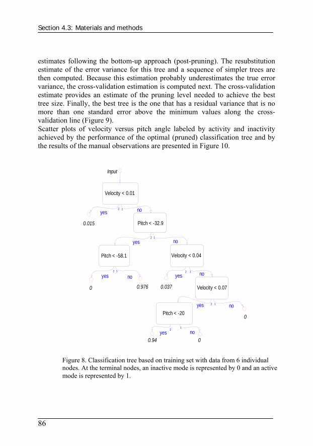
Section 4.3: Materials and methods

86

estimates following the bottom-up approach (post-pruning). The resubstitution estimate of the error variance for this tree and a sequence of simpler trees are then computed. Because this estimation probably underestimates the true error variance, the cross-validation estimation is computed next. The cross-validation estimate provides an estimate of the pruning level needed to achieve the best tree size. Finally, the best tree is the one that has a residual variance that is no more than one standard error above the minimum values along the cross-validation line (Figure 9). Scatter plots of velocity versus pitch angle labeled by activity and inactivity achieved by the performance of the optimal (pruned) classification tree and by the results of the manual observations are presented in Figure 10.

Figure 8. Classification tree based on training set with data from 6 individual nodes. At the terminal nodes, an inactive mode is represented by 0 and an active mode is represented by 1.

Velocity < 0.01

Pitch < -32.9

Pitch < -58.1 Velocity < 0.04

Velocity < 0.07

Pitch < -20

0.015

0 0.976 0.037

0

00.94

Input

no1yes

2

no1

yes2

no1

yes2

yes2 no1

yes 2 no1

yes2 no

1

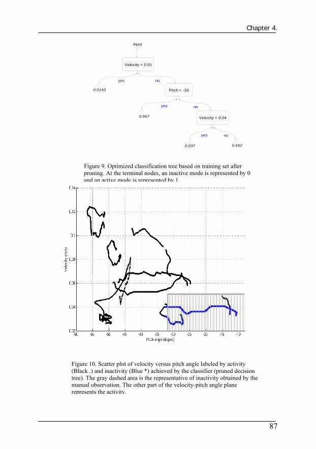
Chapter 4.

87

Figure 9. Optimized classification tree based on training set after pruning. At the terminal nodes, an inactive mode is represented by 0 and an active mode is represented by 1.

0.0143 Pitch < -33

Velocity < 0.040.957

0.037 0.652

Input

Velocity < 0.01

yes

2

no

1

no

1

yes

2

no

1

yes

2

Figure 10. Scatter plot of velocity versus pitch angle labeled by activity (Black .) and inactivity (Blue *) achieved by the classifier (pruned decision tree). The gray dashed area is the representative of inactivity obtained by the manual observation. The other part of the velocity-pitch angle plane represents the activity.

Section 4.4: Results

88

IV. Results Table 1 represents the results of behavior classification in which the ground-truth was achieved by manual observation carried out during the experiment. The procedure consisting of training, pruning and validation was performed 6 times. Each time, 6 randomly chosen datasets out of the 8 were used for training and pruning while the remaining 2 datasets were used for validation. It is assumed that each dataset was associated with an animal therefore the dataset associated with cow )4,3,2,1(=a in day )2,1(=q was defined as aqT or '

aqT in case that dataset was used in training set or in validation set respectively. The measurements of pitch angle and velocity were used as predictors and the behavior classified as activity or inactivity was used as the response. It can be concluded from the table that a general classification tree as shown in Figure 9 constructed by the data from a subset of cows could predict the behavior of other cows with high classification success rate. Similar classification tables have been achieved by only considering the pitch angle or velocity as the predictor but the classification results showed much lower success rates in comparison to the results of Table 1. Constructing the tree only based on pitch angle measurements as the predictor showed that the classification tree could predict the behavior with 55% success rate while the velocity as the unique predictor could classify the behavior with 43% accuracy on average. Based on manual registration and GPS measurements, cow2 associated with node2 was the most active cow (92% of time active) in the group. It can be seen in the Table 1, the classification success rate is minimum when the data of cow2 is not considered for training the tree. Cow1, on the other hand, was the most inactive cow in the group (83% of time active) and hence has limited effect on training the tree. As the evaluation criterion most used for a classifier is the error rate (the ratio of the number of falsely classified samples to the whole number of samples), this rate has been calculated for the pruned decision tree shown by Figure 9, a trained fuzzy logic classifier and a trained neural network classifier. Furthermore, the classification cost in terms of number of nodes or neurons were taken as well into account. While a simple classification tree with 4 terminal nodes could classify the behavior with error rate of 16.76 % on average, the same data sets were imported to the fuzzy logic classifier and the error rate of 19.32% was achieved by 70 trained epochs and in the case of linear neural network classifier, the error rate of 18.65% was achieved by 100 neurons.

Chapter 4

89

Table 1. Classification success rate using cross validation method, representing the accuracy to predict the behavior of some cows using the behavior of other cows in the same herd

trainT validationT Classification success rate

T11, T21, T31, T12 ,T22 ,T42

T´41 T´32

83.2% 80%

T11 ,T21, T31, T22, T32, T42

T´41 T´12

80.5% 95.1%

T11, T21, T41, T22, T32, T42

T´31 T´12

82% 93.4%

T11, T31, T41, T12, T32, T42

T´21 T´22

71.8% 70.2%

T21, T31, T41, T12, T32, T42

T´11 T´22

84.3% 72.6%

T21, T31, T41, T22, T32, T42

T´11 T´12

90.3% 95.5%

V. Conclusions Pitch angle measurements as well as movement velocity estimation were successfully transmitted through a wireless sensor network and were used to classify the animal behavior into two classes as active and inactive. The proposed Kalman filter could handle the problem raised by packet loss due to intermittent observation by estimating the lost states. The problem of non representative local peaks due to head movements during grazing period were addressed and robustly solved by a Kaiser window. Classification trees showed advantages over neural network and fuzzy logic classifiers therefore a general classification tree was preferred. The classification tree was constructed based on the measurements of pitch angle of the neck and the movement velocity. The results showed that there was a large improvement in the classification accuracy if both pitch angle of the neck and velocity were employed as predictors in comparison to just pitch angle or just velocity employed as the single predictor. The results suggest that a classification tree for behavior classification was a compromise between active and less active cows. In spite of this, it seemed that

Section 4.5: Conclusions

90

success rate of at least 70.2% could be achieved. The results have been confirmed by manual registration and by GPS measurements. To confirm or reject this percentage, a study including more cows during more days is necessary. The classification results proved the possibility of determining a general decision rule (model) which can classify the behavior of each individual in a herd of animals. Consequently, the achieved behavioral model could then be used for further control purposes such as behavioral control. However the classification results showed an improvement compared to the results achieved by other studies, some key challenges such as a more robust wireless sensor network, with less percentage of packet loss, and more precise methods to estimate the movement velocity are required.

Reference

Analog device dataste (2007). ADXL202JE accelerometer data sheet. Arias J; Zuloaga A; Lazaro J; Andreu J; Astarloa A. (2004). Malguki: an

RSSI based ad hoc location algorithm. Journal of Microprocessors and Microsystems, Vol. 28, pp. 403-409.

Ashan S; T. (2003). Optimal window design. Journal of IEEE potentials, Vol21, Issue 5, pp. 39-43

Breiman L. (1998). classification and regression tree. Boca Raton, Fla.: Chapman & Hall/CRC.

Butler Z; Corke P; Peterson R; Rus D. (2004). Networked Cows: Virtual Fences for Controlling Cows. International Conference on Robotics and Automation, (ICRA)

Elnahrawy E; Li X; Martin R P (2004). “The Limits of Localization Using Signal Strength: A Comparative Study”, in Proceedings of the First IEEE International Conference on Sensor and Ad hoc Communications and Networks (SECON).

Gay D; Levis P; Culler D (2007). Software Design Patterns for TinyOS. ACM Transactions on Embedded Computing Systems (TECS), Vol. 6, Issue 4.

Harter A; Hopper A; Steggles P; Ward A; Webster P. (1999). The anatomy of a context-aware application, Mobile Computing and Networking, pp. 59–68.

Chapter 4

91

Kotanen A; Hannikainen M; Leppakoski H; Hamalainen T D (2003). Experiment on local positioning with Bluetooth. Information Technology: Coding and Computing [Computers and Communications], 2003. Proceedings. ITCC 2003. International Conference, pp. 297 - 303

Munksgaard L; Jensen, M.B; Herskin, M.S; Levendahl, P; 2005. The need for lying time in high producing dairy cows. Proc. 39th Int. Congress of the ISAE, Kanagawa, Japan, 38.

Nadimi E S; Bak T; Izadi-Zamanabadi R (2006). Monitoring animals and herd behavior parameters using a wireless sensor network. Proceedings of XVI CIGR world congress. Book of abstracts, pp. 415-416.

Nadimi E S; Søgaard H T; Oudshoorn F W; Blanes-Vidal V; Bak T (2007). Monitoring Cow Behavior Parameters based on Received Signal Strength using Wireless Sensor Networks. 3rd European conference on precision livestock farming. Greece.

Nielsen C; Kracht S; Svenstrup M. 2005. Localization using received signal strength indicator. Report, Aalborg University.

Oppenheim A V; Schafer R W; Buck J R (1999). Discrete-time signal processing. Upper Saddle River, N.J.: Prentice Hall. ISBN 0-13-754920-2.

Oudshoorn F; Kristensen T; Nadimi E S (2006). Dairy cow defecation and urination frequency and spatial distribution related to time limited grazing, accepted in the journal of livestock production sciences.

Polastre J. (2003) Design and Implementation of Wireless Sensor Networks for Habitat Monitoring. Master’s thesis, University of California, Berkeley.

Priyantha N B; Chakraborty A; Balakrishnan H (2000). The Cricket Location-Support System, Mobile Computing and Networking, pp.32–43.

Sallvik K; Oostra H.H. 2005. Automatic Identification and Determination of the Location of Dairy Cows, Precision Livestock Farming ‘05, edited by S. Cox.

Schetinin V; Fieldsend J E; Partridge D; Krzanowski W J; Everson R M; Bailey T C; Hernandez A (2004). The Bayesian Decision Tree

References

92

Technique with a Sweeping Strategy. International Conference on Advances in Intelligent Systems - Theory and Applications, Centre de Recherche Public Henri Tudor, Luxembourg-Kirchberg, Luxembourg, November, 2004.

Schwager M; Anderson M. D.; Butler Z; Rus D (2007). Robust classification of animal tracking data, Computers and Electronics in Agriculture, Vol. 56, Issue 1, pp. 46-59.

Sinopoli B; Schenato L; Franceschetti M; Poolla K; Jordan M.I; Sastry S.S. 2004. Kalman filtering with intermittent observation. IEEE transaction on automatic control, Vol. 9, pp. 1453-1464.

Szewczyk R; Osterweil E; Polastre J; Hamilton M; Mainwaring A; Estrin, D. 2004. Habitat monitoring with sensor networks. Journal of Communications of the ACM, Vol.47, issue 6, pp.34-40.

Umstatter C; Waterhouse A; Holland J. 2006. An automated method of simple behavior classification as a tool for management improvement in extensive systems. 4th international workshop on smart sensors in livestock monitoring. Book of abstracts, pp.57-58

Ward A; Jones A; Hopper A. (1997). A new location technique for the active office. IEEE Personal Communications, pp.42–47.

Wark T; Crossman C; Hu W; Guo Y; Valencia P; Sikka P; Corke P; Lee C; Henshall J; Prayaga K; O’Grady J; Reed M; Fisher A. (2007). The Design and Evaluation of a Mobile Sensor/Actuator Network for Autonomous Animal Control. Proceedings of the 6th international conference on Information processing in sensor networks. pp. 206 – 215; ISBN: 978-1-59593-638.

White S L; Sheffield R E; Washburn S P; King L D; Green J T (2001). Spatial and Time Distribution of Dairy Cattle Excreta in an Intensive Pasture System, journal of ENVIRON. QUAL, Vol.30, November-December 2001.

Wilson S C; Dobos R C; Fell L R (2005). Spectral analysis of feeding behavior of cattle kept under different feedlot conditions”. Journal of Applied Animal Welfare science.

Zhang P; Sadler C. M; Lyon A. S; Martonosi M. (2004). Hardware Design Experiences in ZebraNet. Proceedings of the 2nd international conference on Embedded networked sensor systems. pp. 227 – 238. ISBN: 1-58113-879-2

CHAPTER 5 Observer Kalman filter identification and multiple-model adaptive estimation for classifying animal behavior using wireless sensor networks

Section 5.1: Introduction

94

Observer Kalman filter identification and multiple-model adaptive estimation for classifying animal behavior using

wireless sensor networks

E. S. Nadimia,b,* , H. T. Søgaardc, T. Bakb

aResearch Center Bygholm, Department of Agricultural Engineering,

Aarhus University, Denmark bDepartment of Electronic Systems, Automation and Control, Aalborg

University, Denmark Engineering College of Aarhus, Aarhus, Denmark

Abstract: The identification of a mathematical model capable of precisely describing the behavior of animals given input such as feed has great potential for behavioral control purposes. Such models will provide a prediction capability which is fundamental to any closed loop control of the behavior e.g. control the feeding. This paper investigates the problem of mathematically modeling animal behavior that is feeding activity or feeding inactivity of dairy cattle given feed dry matter. The observer-Kalman filter identification method was successfully applied to input-output data and two models representing the hypothesis that animals are actively feeding and the hypothesis that animals are inactive were identified. The input and output of each of the identified models was feed dry matter offer and the pitch angle of the neck respectively. The pitch angle of the neck of the animal was successfully measured and aggregated by a ZigBee-based wireless sensor network. Two forth-order models describing the dynamics of an animal in the active and inactive behavior modes showed precise performance in terms of prediction error, cross correlation function between residual and the output as well as cross correlation between residual and the input with 97% confidence interval. Each of the two models describes different biological behavior hypothesis (active and inactive) and a multiple-model adaptive estimation approach was applied to determine the likelihood of each of the two models being the correct model for a specific input of dry matter feed. The minimum achieved classification success rate was 79.7% and the average success rate was 87.2% for the whole experiment. In order to qualify the results of the presented research, more experiments with longer time periods including bigger herds of animals are required, however the results showed great improvement compared to the results of other studies.

Chapter 5

95

Keywords: observer, Kalman filter, multiple-model adaptive estimation, animal behavior, wireless sensor networks

1. Introduction: Modeling of animal behavior plays a fundamental role in the design of systems for monitoring and controlling animal behavior. Such systems can potentially have a significant impact on practical farming by improving animal welfare and livestock management. Appropriate models may be used as predictors in a closed loop setup, where feed is automatically made available based on set references for feeding activity. If e.g. cows do not exhibit an active feeding behavior for sufficient amount of time, optimal production require that more feed be made available to increase the time they spend feeding. If the time they spend actively feeding can be predicted as a basis of the available feed, this may be used to adjust the feeding process automatically. Although different aspects of animal behavior are well known by scientists, it is worth noting that the problem of controlling the behavior of a herd of animals by controlling the environment (e.g. the feed) is still far from being resolved in an optimal way. One of the main reasons for that is that the dynamic behavior of animals and their interaction with the surrounding is very complex and difficult to model mathematically in a reliable way that is suited for on-line applications. Among all different aspects of animal behavior which have been studied by different researchers (Szewczyk et al., 2004; Wilson et al., 2005; Guo et al., 2006; Munksgaard et al., 2006; Bishop-Hurley et al., 2007; Oudshoorn et al., 2007; Nadimi et al., 2007; Schwager et al., 2007), grazing behavior has got special attention due to close correlation to animal welfare, productivity and farm management (Wang et al., 2006). In order to be able to study and control the grazing behavior dynamics, a model which could precisely generate the same pattern as actual behavior must be achieved. Such a model (random walk mobility model, random waypoint mobility model, random direction mobility model and Gauss-Markov mobility model) can be found in literature as in Camp et al., 2002. While all these models mainly focus on the motion characteristics (random speed and random direction), a new perspectives to solve the problem of online monitoring of grazing behavior were introduced by Nadimi et al., 2007 and Schwager et al., 2007. In order to evaluate the grazing behavior, parameters such as the pitch angle of the neck of animal in addition to the motion characteristics were registered by wireless sensor networks. In the research carried out by Nadimi et al., 2007 the pitch angle of the neck was modeled by a discrete time Wiener process and subsequently translated to a behavioral mode (active or inactive). Lack of deterministic inputs (time series) in the Wiener process as well as

Section 5.1: Introduction

96

inaccurate achieved results led to inapplicability of Wiener process for further control purposes. Therefore a model of the grazing behavior in terms of activity and inactivity taking the pitch angle of the neck into account as output and providing the information of an input (i.e. dry matter offer) into the model would be of interest. The Observer Kalman filter identification (OKID) method is one of the time domain techniques relevant for this problem as no a priori knowledge of the system is needed. Input-output data is sufficient, and a pseudo-Kalman filter state estimator is produced making it very useful for control applications (Elkaim, 2002). Furthermore, the technique has been proven to be numerically efficient and robust with respect to measurement noise and even in the presence of mild nonlinearities (Tiano et al., 2007). Thus in the present research, the OKID method has been applied and two different state space models that describe the animal dynamics in terms of pitch angles of the neck were identified. The use of two models reflects observations on animals that indicate significant differences in the neck pitch dynamics given the behavioral mode of the animal. An animal grazing is moving its head up and down in a periodic manner, whereas the dynamics of the head movement of an animal resting etc. has much lower frequency content. The two models reflect this observation by assuming two different hypotheses. One model reflects the hypothesis that the animal is grazing, while the other reflect the hypothesis that the animal is not grazing. To determine the likelihood of a given model and thereby hypothesis being the correct, the models are fused with a multiple-model adaptive estimation approach (Bak, 2000; Ferreira & Waldmann 2007). The two dynamic models combined with multiple-model adaptive estimation allow a classification of the activity mode of the animal into grazing or non-grazing. Different classification methods such as decision trees, fuzzy logic, neural networks, K mean classifier and multiple-model adaptive estimation (MMAE) have been implemented in different applications (Bak 2000, Bar-shalom and Fortmann 1988, Ormsby 2003, Nadimi et al., 2007, Ferreira and Waldmann 2007, Schwager et al., 2007). To the authors’ best knowledge, among the classification methods, MMAE has not been implemented in animal behavior studies. One reason for that could be lack of reliable and suitable models describing the dynamic behavior of animals. In the MMAE method the likelihood of a number of independent dynamic models are continuously evaluated based on their prediction accuracy. The remainder of the paper is organized as follows. The mathematical basis of the observer Kalman filter identification approach will be presented in Section 2. Section 3 is dedicated to the mathematical formulation of multiple-model adaptive estimation approach to evaluate the likelihood of animal behavioral

Chapter 5

97

mode (activity and inactivity). The experimental set up and materials employed in this research are described in section 4. In section 5, the results of system identification and classification using OKID method and MMAE approach are presented respectively. At the end, the conclusions and the discussions of the study are represented.

2. Observer Kalman filter identification method To perform system identification, several methods have been developed over the years (Ljung 2000). Observer Kalman filter identification (OKID) is a time domain technique with several advantages for the specific application addressed in this paper. First, OKID technique assumes that the system in question is a discrete linear time invariant (LTI) state space system. Second, only input and output data to formulate the model is required and no a priori knowledge of the system is needed. Third, the OKID method produces a pseudo-Kalman state estimator, which is very useful for control applications and at last, the truncation errors are small, thus even in the case of model order error, the results of that error will be minimal (Elkaim, 2002). Consider a system described by an LTI discrete time multiple-input, multiple-output (MIMO) state space model of the form:

⎩⎨⎧

+=+=+

)()()()()()1(

kDukCxkykBukAxkx

(1)

with input vector mRku ∈)( , output vector pRky ∈)( , state vector

nRkx ∈)( , and system matrices nnRA ×∈ , mnRB ×∈ , npRC ×∈ and mpRD ×∈ .

The identification problem consists of determining the minimal state space realization using input-output discrete data { } mN

k Rku ∈=0)( , { } pNk Rky ∈=0)(

which means that the dimension of state space vector ( n ) as well as system matrices DCBA ,,, have to be identified. According to the OKID algorithm (Juang, 1994), to artificially increase the damping of the system, an observer is applied to state Eq. (1), by using an observer gain matrix pnRG ×∈ .

[ ]⎩⎨⎧

∈−+=

+=+× )()()( pmnRGGDBB

GCAA (2)

Section 5. 2: Observer Kalman filter identification method

98

Therefore the state space model presented in Eq. (1) can be rewritten as equation below:

⎪⎪⎪

⎩

⎪⎪⎪

⎨

⎧

∈⎥⎦

⎤⎢⎣

⎡=

+=+=+

+ pmRkyku

kv

kDukCxkykvBkxAkx

)()(

)(

)()()()()()1(

(3)

where in Eq. (3), )(kv is an extended input vector. The matrix G can be chosen to make A as stable as desired, under an observability condition, i.e. all the eigenvalues of the modified system can be arbitrarily placed inside the unit circle. Eq. (3) is an observer equation if the state vector )(kx is considered as an observer state vector, therefore the Markov parameters of the system in Eq. (3) will be referred to as observer Markov parameters (Tiano et al., 2007). To select the observer gain matrix G such that all the eigenvalues of A are placed inside the unity circle, a P step ahead predictor for output vector in response to arbitrary initial conditions and input values could be formulated as Eq. (4).

VY θ= (4)

[ ][ ]

⎥⎥⎥⎥

⎦

⎤

⎢⎢⎢⎢

⎣

⎡−++

+++

=

=

+++=−

)()2()1(

)1()1()()()2()1(

)()2()1(1

Lvvv

LPvPvPvLPuPuPu

V

BACBCDLPyPyPyY

P

K

MOMM

K

K

K

K

θ

In Eq. (4), Y is a set of L predicted output values, V is extended input matrix and θ is the vector of observer Markov parameters (Juang, 1994). Assuming that the input is persistently exciting, the observer Markov parameters can be determined as follows:

Chapter 5

99

[ ] +== VYPθθθθθ L210 (5) where +V is the pseudo-inverse of V and kθ is defined as in Eq. (6).

[ ] [ ])2()1(111 )()()( kkkkk

k GGCACGDBGCACBAC θθθ =+−++== −−− (6)

In order to have a unique solution, all the rows of V must be linearly independent. Furthermore, to minimize any numerical error due to the computation of the pseudo-inverse, the rows of V should be chosen as independently as possible (Juang, 1994). As a result, the maximum value (upper bound of the order of the deadbeat observer) of the prediction horizon ( P ) can be described as in Eq. (7).

mpmLP

+−

≤ (7)

Once the vector of observer Markov parameters has been identified, the system matrices ( DCBA ,,, ) and the order of minimum realization can be determined. For this purpose, the eigensystem realization (ERA) could be employed in which the generalized Hankel matrix composed of observer Markov parameters should be formed as in Eq. (8).

[ ]BABABA

AC

ACC

kH ssk

ssssksskssk

sskkk

sskkk

11

1221

21

11

)1( −−

−−++−+

+++

−++

⎥⎥⎥⎥

⎦

⎤

⎢⎢⎢⎢

⎣

⎡

=

⎥⎥⎥⎥

⎦

⎤

⎢⎢⎢⎢

⎣

⎡

=− LM

L

MOMM

L

L

θθθ

θθθθθθ

(8)

in which ss should be chosen much larger than the expected state vector dimension ( n ). Factorization of the block data matrix using singular value decomposition in Eq. (8) for 1=k would result in an equation as presented in Eq. (9).

TSRH ∑=)0( (9) where the columns of matrices R and S are orthonormal and ∑ is a rectangular matrix as presented in Eq. (10).

Section 5. 2: Observer Kalman filter identification method

100

0),,,(000

2121 ≥≥≥≥=∑

⎥⎦

⎤⎢⎣

⎡∑=∑

nnn

n

wherediag σσσσσσ LL

(10)

While the diagonal elements of n∑ correspond to the robustly controllable and observable system state components, the other singular values are correspondent to the measurement noise (Tiano et al., 2007). Therefore, to eliminate the high-frequency contamination, the measurement data should be pre-filtered before any model parameters could be identified. Assuming that the true system could be represented by )(sH , A good estimation of the state vector dimension ( n ) should qualify certain condition as introduced by Eq. (11).

⎪⎪⎩

⎪⎪⎨

⎧

∑≤

−−

∑≤−−

∞

∞

−∞

−

1

1

1

)(2)(

)()(

)(2)()(

σn

n

tracesH

BAsICsH

traceBAsICsH

(11)

Taking Eq. (9) to (11) into consideration, the Eq. (9) can be rewritten as follows:

Tnnn SRH ∑=)0( (12)

where matrices nR and nS are constructed by the first n columns of R and S respectively. Hence, the estimation of system matrices can be achieved as presented in Eq. (13).

½

½

½½ )1(

nnTm

rTnn

nnTnn

REC

ESB

SHRA

∑=

∑=

∑∑= −−

(13)

in which the definition of matrices rE and mE are shown in Eq. (14).

[ ][ ]ppp

Tm

pmpmpmTr

IE

IE

00

00

L

L

=

= +++ (14)

Chapter 5

101

Using Eq. (13) and (14), the observer gain matrix G and system matrices ( CBA ,, ) can be obtained (Juang, 1994). Another straight forward approach to identify system matrices using observer Markov parameters could be obtained by the general relationship between the actual system Markov parameters and the observer Markov parameters by inducing Eq. (2), (5) and (8) as described in Eq. (15).

∑∑

= −

= −

∞+=−=

=−=

=

P

i ikik

k

i ikikk

Pk

Pk

D

1)2(

1)2()1(

0

,,1

,,2,1

L

L

θθθ

θθθθ

θ

(15)

Applying the Eigensystem Realization Algorithm (ERA) to the system Markov parameters would consequently result in achieving the system matrices (Elkaim, 2002).

3. Multiple-model adaptive estimation approach While a complex model relies on several assumptions to describe the actual system, it can only provide more accurate estimates in very specific situations compared to the results achieved by employing several simple models (Bak, 2000; Ferreira & Waldmann 2007). Multiple-model adaptive estimation (MMAE) uses a number of models and calculates the likelihood of each model and their combinations to yield the (sub)optimal estimate. Over time, suitable models would have high probabilities and therefore dominate the estimates (Ferreira and Waldmann 2007). The fundamental basic of MMAE used in the present research is shown in Figure 1 (Ferreira and Waldmann 2007).

Section 5. 3: Multiple-model adaptive estimation approach

102

MMAE mainly relies on two assumptions. The first assumption is that the true model is among the proposed models and the second one is that the same true model has been running since 0=t (Bak, 2000; Ferreira & Waldmann 2007). Let )(kiμ be the probability that the MMAE method attributes to model

)2,1( =iM i at time kt = given the measurements up to that time ),,( 0 kk yyY K= (Eq. (16)).

)),(()()( 1−=Δ kikii YkyMpYMpkμ (16)

The initial probability )0(iμ that a given model iM is the correct one is defined by a priori information. The updating process from )1( −kiμ to )(kiμ can be achieved using Eq. (17).

Classification

Kalman filter Activity model

Kalman filter Inactivity model

MMAE approach

Probability calculation

Output data

Input data

Figure 1. Fundamental basics of MMAE approach.

Probabilities of activity and inactivity model

Measurements residual

Measurements residual

Chapter 5

103

∑=

−

−

−

−−

−

−== 2

11

1

1

11

)1(),)((

)1(),)(())((

)(),)(()(

jjjk

iik

k

kiiki

kMYkyp

kMYkypYkyp

YMpMYkypk

μ

μμ (17)

Let the likelihood function )(kjλ be the conditional probability density

function ),)(( 1 jk MYkyp − that observation )(ky occurs assuming the

validity of model jM . The likelihood can be extracted directly from the

innovation process (residual measurements )(krj ) in the j th Kalman filter

assuming that it is Gaussian, zero mean and with covariance jS . Therefore,

)(kjλ can be defined as follows in Eq. (18) (Bak, 2000; Ferreira & Waldmann 2007).

)21exp(

)2(

1),)(()( 1½2/1 jj

Tj

jpjkj rSr

SMYkypk −

− −==π

λ (18)

Using Eq. (17) and (18), the probability )(kiμ that model iM is correct is updated by using Eq. (19).

∑=

−

−= 2

1)1()(

)1()()(

jjj

iii

kk

kkk

μλ

μλμ (19)

4. Experimental setup and materials The case study in the presented experiment was a group of dairy cows. In order to monitor behavior parameters of the herd, MPR2400 Micaz sensor motes from Crossbow were employed. They have a Chipcon CC2420 radio, which uses a 2.4 to 2.48 GHz IEEE 802.15.4/ZigBee RF transceiver with MAC support. They include direct sequence spread spectrum (DSSS) radio which is resistant to RF interference and provides inherent data security. TinyOS as the operating system was running on the motes. MTS310 sensor board equipped with a 2-axis accelerometer was employed to measure the pitch angle of the neck of each cow. A cow with the head down

Section 5. 4: Experimental setup and materials

104

would nominally register with a pitch angle of -40 degrees and a cow with its head upright would register with a pitch angle of -10 degrees. The accelerometer readings together with the sensor ID were encapsulated in one packet. The selected sampling rate for the packet dissemination was 1 Hz (Nadimi et al., 2007). Multiple sensor nodes sent sensor readings to a base station or aggregation point in the network (gateway) using many to one routing protocol. The gateway was an MIB600 which provided a TCP/IP interface for both programming and data communication. The CC2420 radio supports up to 255 different transmission power levels and allows for a programmable transmission frequency. In order to minimize the number of variables in the experiment, the RF transmission frequency and the transition power were respectively fixed at a single frequency band (2.48 GHz) and at the maximum transmission power (1 mW). The selection of the radio channel 26 (associated with frequency band 2.48 GHz) could be justified due to the highest packet delivery performance in this radio channel while the maximum transmission power was chosen because the maximum communication range was achieved. The experiment was carried out over 3 days with 4 cows 6 hours per day on average. The cows were equipped with wireless nodes around the neck. The node on the collar as well as the collar itself was fixed very well to prevent any slide to right or left side. The antenna pointed to the sky in order to have better communication between nodes and the gateway. The antenna was ½ wave dipole antenna, with an MMCX connector. The gateway was installed 1.2 m above the ground. The shape of the field was rectangular and the area was 60 m long by 40 m wide. Each day, a new field with the same dimension (60 m by 40 m) covered by new grass was provided for the cows. Manual registrations of the absolute time of the day as well as the behavioral mode (active or inactive) of each cow were carried out during the whole day. During the experiment, the grass length (dry matter offer) was measured in different parts of the field and the average length was chosen to express the general grass length and thereby dry matter offer.

5. Results

5.1 OKID identification results The OKID method assumes that the system to be identified is LTI. Another requirement for the implementation of the OKID method is to have close to noise-free data. To reduce the measurement noise of the neck pitch angle measurements they were filtered by a low pass filter (rectangular window). The

Chapter 5

105

window length ( 3=W seconds) was chosen in order to be able to capture the dynamics of the head movements. Based on field observations and manual registrations, the animals move the head with a frequency of 1 Hz during the active period. Therefore, to design a low pass filter capable of removing high frequency contamination (noise) and keeping the fluctuations of 1 Hz, the maximum window length should be 6 seconds ( W

π2 ). Consequently, the

window length was selected to ensure that the head fluctuations would be detected. Applying the designed low pass filter to the pitch angle measurements resulted in the filtered data as exemplified by Figure 2 (a). In order to properly identify the parameters of the model relating the pitch angle of the neck (output) to dry matter offer (input), the input signal should be persistently exciting (Ljung and Soderstrom, 1986; Ljung, 1987). The input signal was modeled as a ramp signal with an additive random process, based on two facts: (1) The manual registrations demonstrated that dry matter offer descends with negative slope with increasing time (Oudshoorn et al., 2007) and (2) The grazing process is an irregular process, as the animals stop grazing time to time. Consequently, a random process was added to the ramp signal in such a way that at each time step, the dry matter offer is larger or equal than the dry matter offer of the next time step. Therefore, the manual registrations of the dry matter offer were resampled and random process with mean value (0) and small standard deviation (0.001) compared to the mean value and the standard deviation of the input signal, was added to the input signal. As a consequence of adding a random signal with mean value (0) to the input signal, the identification process would be unbiased (Ljung and Soderstrom, 1986; Ljung, 1987). Therefore the input signal was filtered as well, by a rectangular window in order to remove the high frequency contamination and to ensure that the low frequency components of the measurements of the dry matter offer (input) would be kept. The new input signal used in the identification process is presented by Figure 2 (b). As a single complex model can provide accurate estimates of the system in specific situations compared to the results achieved by several simple models, the output data set as well as input data set was divided to 2 datasets, one representing the active period ( AP ) when the animal is grazing and the other one representing inactive period ( IP ) when it is not. The division process of the output and input data set were carried out according to the manual registration of the behavior as observed during the experiment. Each data set representative of activity or inactivity was divided into two subsets for identification process ( II IPAP , ) and validation process ( VV IPAP , ). Later on,

Section 5.5: Results

106

the OKID method was applied to each data set ( II IPAP , ) and two dynamic models were obtained. As the first step in the OKID algorithm, an appropriate prediction horizon ( P ) using Eq. (7) should be selected. Taking into account that the system is single-input single-output (SISO), by implementing Eq. (7), P has been selected as 30 samples. Identifying the observer Markov parameters of the active and inactive period associated with the data sets IAP and IIP and forming the Hankel Matrix resulted in singular value decomposition as presented by Figure 3.

0 1 2 3 4 5 6-100

-80

-60

-40

-20

0

Time (Hour)

Pitc

h an

gle

of th

e ne

ck (D

egre

e) (a)

0 1 2 3 4 5 6160

180

200

220

240

260

Time (Hour)

Dry

mat

ter o

ffer (

Kg)

(b)

Figure 2. Filtered measurements of the pitch angle of the neck (output of the process) using a low pass filter (rectangular window with window length = 3 sec) (a). Dry matter offer as the input of the process (b).

Chapter 5

107

Taking Eq. (11) and Figure 3 into account would reveal that a forth or higher order model is in perfect agreement with the input-output data. However, fifth or higher order models have been rejected since pole-zero cancellation would suggest that it could be a consequence of round-off modeling errors. By identifying system matrices, the eigenvalues of the models associated with activity and inactivity could be calculated (Figure 4). As a subset of each data set ( II IPAP , ) was specified to the identification process, validation process was carried out on the other subsets ( VV IPAP , ). The results of the validation process are shown by Figure 5 in terms of the difference between model output and the measurements (one step ahead prediction error). The absolute mean value of the prediction error for the activity period and inactivity period was 1.8 and 0.6 degrees on average respectively. The prediction error time series (cross correlation between residuals and the output) of the identified activity state model with 97% confidence interval is presented by Figures 6 and 7. The cross correlation of the input and output residuals is presented as well (97% confidence interval) by the same Figures (6

0 5 10 150

0.2

0.4

0.6

0.8

Number

Sin

gula

r val

ue m

agni

tude

(act

ivity

)

0 5 10 150

0.05

0.1

0.15

0.2

Number

Sin

gula

r val

ue m

agni

tude

(ina

ctiv

ity)

Figure 3. Singular value magnitude of the identified models for activity state

Section 5.5: Results

108

and 7). It can be confirmed that the identified models showed a good prediction capability as the cross correlation functions are within the 97% confidence interval.

0 50 100 150 200 250 300 350 400-10

-5

0

5

10

Time (Sec)

Pre

dict

ion

erro

r for

act

ive

perio

d (D

egre

e)

0 50 100 150 200 250 300 350 400-6

-4

-2

0

2

4

6

Time (Sec)

Pre

dict

ion

erro

r for

inac

tive

perio

d (D

egre

e)

Figure 5. Prediction error achieved in the validation process for activity phase (upper) and inactivity phase (lower).

-0.2 0 0.2 0.4 0.6 0.8 1-0.5

-0.4

-0.3

-0.2

-0.1

0

0.1

0.2

0.3

0.4

0.5

Real axis

Imag

inar

y ax

is

Figure 4. Eigenvalues of the models associated with activity state. The star represents the eigenvalues of the model in terms of activity and the plus

represent the eigenvalues of inactivity model.

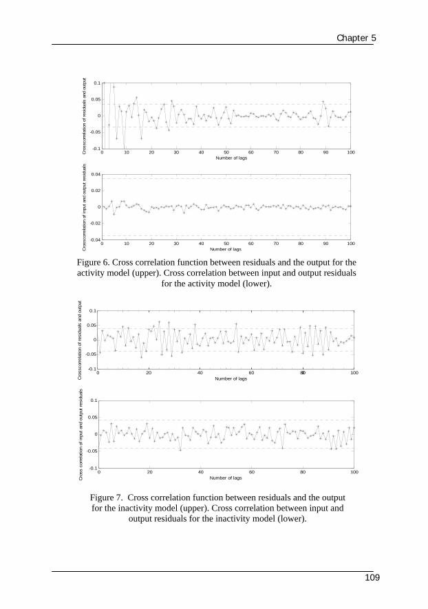
Chapter 5

109

0 10 20 30 40 50 60 70 80 90 100-0.1

-0.05

0

0.05

0.1

Number of lags

Cro

ssco

rrela

tion

of re

sidu

als

and

outp

ut

0 10 20 30 40 50 60 70 80 90 100-0.04

-0.02

0

0.02

0.04

Number of lagsCro

ssco

rrela

tion

of in

put a

nd o

utpu

t res

idua

ls

Figure 6. Cross correlation function between residuals and the output for the activity model (upper). Cross correlation between input and output residuals

for the activity model (lower).

0 20 40 60 80 1000-0.1

-0.05

0

0.05

0.1

Number of lagsCro

ssco

rrela

tion

of re

sidu

als

and

outp

ut

0 20 40 60 80 100-0.1

-0.05

0

0.05

0.1

Number of lagsCro

ss c

orre

latio

n of

inpu

t and

out

put r

esid

uals

Figure 7. Cross correlation function between residuals and the output for the inactivity model (upper). Cross correlation between input and

output residuals for the inactivity model (lower).

Section 5.5: Results

110

5.2 Multiple-model adaptive estimation results Assuming that the behavioral mode (activity and inactivity) models are represented by 1M and 2M respectively, MMAE approach has been applied to

1M and 2M to calculate the likelihood of each model and their combination to yield the optimal estimate. The initial probabilities )0(1μ and )0(2μ that 1M or 2M is the correct model was defined by a priori information. As it was observed, all the animals were active when the experiment started therefore the initial probabilities )0(1μ and )0(2μ were assigned to 0.6 and 0.4 respectively. Applying Eq. (16) to (19) to the models would result in the probability assignment as shown in Figure 8.

Figure 8. Classification results of activity state using MMAE approach. The top figure represents the pitch angle of the neck; the

figure in the middle is the likelihood function that model 1M is correct while the lowest figure is the likelihood function that model

2M is correct.

0 1 2 3 4 5 6-100

-50

0

Time (Hour)Pitc

h an

gle

of th

e ne

ck (D

egre

e)

0 1 2 3 4 5 60

0.5

1

Time (Hour)

Like

lihoo

d of

act

ivity

mod

el

0 1 2 3 4 5 60

0.5

1

Time (Hour)Like

lihoo

d of

inac

tivity

mod

el

ActiveActive

Active Active

Active ActiveInactive

Inactive

Inactive

Chapter 5

111

From Figure 8 it can be concluded that when the animal was active, the likelihood that model 1M was the correct model would be larger than 0.5 while the likelihood during inactivity period was close to zero. On the other hand, when the animal was inactive, the likelihood that 2M is the correct model would be close to one and during activity period, the likelihood would be smaller than 0.5. Modifications in the likelihood results as proposed by Ferreira & Waldmann 2007 were carried out such that the probabilities larger than 0.5 was assumed as 1 and the probabilities smaller than 0.5 was assumed as zero. As behavioral mode periods of all the animals were registered manually during the experiment (ground truth), the pitch angle measurements of all the animals as well as dry matter offer were fed into the identified activity ( 1M ) and inactivity models ( 2M ) and the results of MMAE approach were achieved and summarized by Table 1. Therefore, the classification success rate in Table 1 was calculated as the percentage of the correct behavior classification (behavioral mode) using MMAE approach compared to the results of manual registrations.

Table 1. Classification success rate achieved by the identified models and MMAE

approach Day No Cow No

No.1

No. 2

No. 3

No. 1

88.2%

81.5%

86.3%

No. 2

89.7%

85.6%

88.4%

No. 3

81.5%

80.3%

79.7%

No. 4

96.8%

96.1%

92.4%

As a result of Table 1, 87.2% success rate was achieved on average which is significantly higher compared to the results of other studies (Nadimi et al., 2007; Schwager et al., 2007, Umstatter et al., 2006); however to confirm the

Section 5.6: Conclusions

112

obtained success rate, more experiments should be carried out in which higher number of animals are monitored during longer periods of time. Conclusions The problem of animal behavior identification in terms of behavioral mode (activity and inactivity) using mathematical models has been addressed. The observer-Kalman filter identification method was successfully applied to input-output data and two models representing the hypothesis that animals are actively feeding and the hypothesis that animals are inactive were identified. The input and output of the identified models was dry matter offer and the pitch angle of the neck respectively. The output was successfully measured and aggregated by ZigBee-based wireless sensor networks. Many-to-one routing protocol was used as the communication protocol between sensor nodes and the gateway. Two forth-order models describing behavioral mode showed precise performance in terms of prediction error, cross correlation function between residual and output as well as cross correlation between residual and the input with 97% confidence interval. The achieved models could be potentially employed for further control purposes. As another objective of the paper was to properly classify the behavior of the animals in terms of activity and inactivity using obtained models, multiple-model adaptive estimation approach has been applied to the input-output data. The achieved minimum classification success rate was 79.7% and the average success rate was 87.2% for the whole experiment. In order to qualify the results of the presented research, more experiments with longer time periods including bigger herds of animals are required, however the results showed great improvement compared to the other studies. References Bak, T. (2000). Lecture notes—estimation and sensor information fusion.

Aalborg, Denmark: Department of Control Engineering, Aalborg University.

Bar-Shalom, Y., & Fortmann, T. E. (1988). Tracking and data association. New York: Academic Press.

Bishop-Hurley, G.J., Swain, D.L., Anderson, D.M., Sikka, P.,Crossman, C., Corke, P., 2007. Virtual fencing applications: implementing and

Chapter 5

113

testing an automated cattle control system. J. Comput. Electron. Agric. 56 (1), 14–22.

Camp, T., Boleng, J., Davies V., 2002. A survey of mobility models for ad hoc network research. Colorado school of Mines.

Elkaim, G., 2002. System Identification for Precision Control of a Wing Sailed GPS-Guided Catamaran. Ph.D. Thesis, Department of Aeronautics and Astronautics, Stanford University.

Ferreira, J. C. B. C., Waldmann, J., 2007. Covariance intersection-based sensor fusion for sounding rocket tracking and impact area prediction. Control Engineering Practice, Volume 15, Issue 4, April 2007, pp. 389-409.

Guo, Y., Corke, P., Poulton, G., Wark, T., Bishop-Hurley, G., Swain, D., 2006. Animal behavior understanding using wireless sensor networks. In: Proceedings of the 1st IEEE International Workshop on Practical Issues in Building Sensor Network Applications (SenseApp 2006), IEEE, Tampa, Fl, pp. 608–614.

Juang, J., N., 1994. Applied system identification. Prentice Hall PTR. ISBN: 0-13-079211-X.

Munksgaard, L., Jensen, M.B., Herskin, M.S., Levendahl, P., 2005. The need for lying time in high producing dairy cows. In:Proceedings of the 39th International Congress of the ISAE, Kanagawa, Japan, pp. 38–42.

Nadimi, E.S., Bak, T., Izadi-Zamanabadi, R., 2006. Monitoring animals and herd behavior parameters using a wireless sensor network. In: Proceedings of XVI CIGR World Congress. Book of Abstracts, pp. 415–416.

Nadimi, E.S., Søgaard, H.T., Oudshoorn, F.W., Blanes-Vidal, V., Bak, T., 2007. Monitoring cow behavior parameters based on received signal strength using wireless sensor networks. In: Cox, S. (Ed.), Proceedings of 3rd European Conference on Precision Livestock Farming (ECPLF)., ISBN 978-90-8686-023-4, pp. 95–103.

Nadimi, E.S., Søgaard, H.T., Bak, T., 2007. ZigBee-based wireless sensor networks for monitoring animal presence and pasture time in a strip of new grass. . J. Comput. Electron. Agric. doi:10.1016/j.compag.2007.09.010.

References

114

Ormsby, C. D. 2003. Generalized Residual Multiple Model Adaptive Estimation of Parameters and States. PhD Thesis. Air force inst of tech wright-patterson afb oh school of engineering and management.

Oudshoorn, F.W., Nadimi, E.S., 2007. Intelligent grazing management using wireless sensor networks. In: Cox, S. (Ed.), Proceedings of 3rd European Conference on Precision Livestock Farming (ECPLF)., ISBN 978-90-8686-023-4, pp. 111–116.

Oudshoorn, F.W., Kristensen, T., Nadimi, E.S., in press. Dairy cow defecation and urination frequency and spatial distribution related to time limited grazing. Livestock Sci., doi:10.1016/j.livsci.2007.02.021.

Schwager, M., Anderson, D.M., Butler, Z., Rus, D., 2007. Robust classification of animal tracking data. J. Comput. Electron.Agric. 56 (1), 46–59.

Szewczyk, R., Osterweil, E., Polastre, J., Hamilton, M., Mainwaring, A., Estrin, D., 2004. Habitat monitoring with sensor networks. J. Commun. ACM 47 (6), 34–40.

Tiano, A., Sutton, R., Lozowicki, A., Naeem, W., 2007. Observer Kalman filter identification of an autonomous underwater vehicle. Control Engineering Practice, Volume 15, Issue 6, June 2007, pp. 727-739.

Wang, N., Zhang, N., Wang, M., 2006. Wireless sensors in agriculture and food industry—recent development and future perspective. J. Comput. Electron. Agric. 50 (1), 1–14.

Wilson, S.C., Dobos, R.C., Fell, L.R., 2005. Spectral analysis of feeding behavior of cattle kept under different feedlot conditions. J. Appl. Anim. Welfare Sci. 8 (1), 13–24.

CHAPTER 6 Conclusions, discussions and future work

Section 1.1: Conclusions

116

It was the goal of the author that throughout the development of this thesis, the design, development and implementation process be sufficiently explained to allow the reader to understand and if desired, enable the reader to replicate the process that resulted in the experimental validation of the project. Indeed, though this thesis describes the process only for a particular implementation of the ZigBee based monitoring system on a group of dairy cows and mathematically model their behavior, it is hoped that it can act as a guide for other applications which apply wireless sensor networks to monitor animal behavior. Conclusions

The problem of animal behavior monitoring and classification in terms of behavioral mode (activity and inactivity) using wireless sensor networks has been successfully addressed in this thesis. The research carried out can potentially result in controlling the animal behavior and consequently improving their productivity and welfare.

Various direct and indirect behavioral parameters (such as location, pH of rumen, position of the neck, status of the leg and the translational velocity) are capable of representing animal behavior. Some of these parameters can indicate the animal behavior in terms of activity and inactivity. Among them, the pitch angle of the neck and the velocity of the movement of the animal were selected in this thesis as indicators of activity and inactivity due to the simplicity of their measurement using non invasive methods and their ability to precisely represent the activity.

In order to measure, aggregate and transmit the behavioral parameters (pitch angle of the neck and the velocity of the movement) through a network to infrastructure facilities, wireless sensor networks demonstrated considerable advantages over other traditional invasive monitoring systems. As using wires is impractical in animal behavior monitoring in outdoor environments and the presence of human can potentially disturb the animal behavior, a wireless remote monitoring system is essential. Among all different wireless based monitoring systems (ZigBee, Bluetooth, RFID and WiFi), a ZigBee based wireless sensor network was selected as it fulfilled all the necessary requirements: bandwidth, short network joining time, long communication range, low energy consumption and low cost. The ZigBee based monitoring system was successfully employed, although the main disadvantage of its use was the relatively high rate packet loss (30% on average) in outdoor environments.

Chapter 6

117

When the behavioral data traveled along unreliable communication channels in the wireless sensor networks, the effect of communication delays and loss of information could not be neglected. Consequently, this problem was addressed by using separate discrete Kalman filters for the registered behavior parameters, in which the arrival of observation packets was modeled as a random process. The lost behavioral parameters data were optimally estimated by the Kalman filter.

Monitoring behavioral parameters of each individual animal in a large herd is necessary when health parameters need to be registered. When the study is focused on activity parameters, monitoring each individual animal is not efficient in terms of time, cost and effort. Therefore, in this thesis, which was focused on animal activity, only a part of the herd (23% of the animals) was equipped with sensor nodes. In order to evaluate whether the monitored animals represented the whole herd, investigations relating the whole herd presence and the registrations of a subset of tagged animals were carried out, indicating that the monitored animals did represent the whole herd in terms of activity.

Given that the tagged animals represented the whole herd, classification of the behavior of the tagged animals into two classes, active and inactive, was carried out. Different classification methods were applied to the data (i.e. pitch angle of the neck and the translational velocity of the animals). Initially, a threshold method was successfully applied to the data using two thresholds defined for behavior classification:

1) A threshold on the pitch angle of the neck (-32 degree). 2) A threshold on the translational velocity (0.05 1−ms ).

Implementing the threshold method resulted in 61% classification success rate. In order to improve the behavior classification, different classification approaches such as decision trees, fuzzy logic and neural network classifiers were successfully applied to the data representing the pitch angle of the neck and the translational velocity of the animals. The best results in terms of error rate and number of nodes were achieved by a pruned decision tree in which both the pitch angle and the translational velocity were selected as predictors. Another advantage of the decision tree was the use of a white-box model, in comparison to fuzzy logic and neural network classifiers (black-box model) in which the explanation of the results can be excessively complex for a decision maker to comprehend. The classification results achieved by the decision tree were improved when both behavioral parameters were utilized as the predictors compared to the classification results when only one of the behavioral parameters was used as the single predictor.

Finally, a high performance Multiple-Model Adaptive Estimation (MMAE) approach to classify animal behavior into two classes, active and

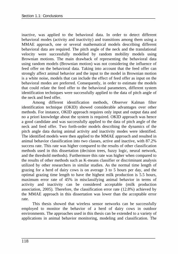
Section 1.1: Conclusions

118

inactive, was applied to the behavioral data. In order to detect different behavioral modes (activity and inactivity) and transitions among them using a MMAE approach, one or several mathematical models describing different behavioral data are required. The pitch angle of the neck and the translational velocity were successfully modelled by random mobility models using Brownian motions. The main drawback of representing the behavioral data using random models (Brownian motion) was not considering the influence of feed offer on the behavioral data. Taking into account that the feed offer can strongly affect animal behavior and the input to the model in Brownian motion is a white noise, models that can include the effect of feed offer as input on the behavioral modes are preferred. Consequently, in order to estimate the models that could relate the feed offer to the behavioral parameters, different system identification techniques were successfully applied to the data of pitch angle of the neck and feed offer.

Among different identification methods, Observer Kalman filter identification technique (OKID) showed considerable advantages over other methods. For instance, OKID approach requires only input and output data and no a priori knowledge about the system is required. OKID approach was hence a good candidate and was successfully applied to the data of pitch angle of the neck and feed offer. Two forth-order models describing the dynamics of the pitch angle data during animal activity and inactivity modes were identified. The identified models were then applied to the MMAE approach and resulted in animal behavior classification into two classes, active and inactive, with 87.2% success rate. This rate was higher compared to the results of other classification methods used in this dissertation (decision trees, fuzzy logic, neural network, and the threshold methods). Furthermore this rate was higher when compared to the results of other methods such as K-means classifier or discriminant analysis utilized by other researchers in similar studies. As the normal time length of grazing for a herd of dairy cows is on average 3 to 5 hours per day, and the optimal grazing time length to have the highest milk production is 5.5 hours, maximum error rate of 45% in misclassifying animal behavior in terms of activity and inactivity can be considered acceptable (milk production association, 2005). Therefore, the classification error rate (12.8%) achieved by the MMAE approach in this dissertation was lower than the acceptable error rate.

This thesis showed that wireless sensor networks can be successfully employed to monitor the behavior of a herd of dairy cows in outdoor environments. The approaches used in this thesis can be extended to a variety of applications in animal behavior monitoring, modeling and classification. The

Chapter 6

119

proposed models describing animal behavior mode can then be used to control the behavior of herds of animals in terms of activity of the animals.

Future work

Having elaborated on the results presented in this dissertation, it is appropriate to outline potential future work. This is presented in the form of future improvements that would potentially enhance the solutions of the problem. Many of the suggested improvements are not difficult and only need sufficient time.

1. Monitoring system

The current configuration of the monitoring system is such that improvements can be made in relation to the following points:

• Packet loss: to design a monitoring system that can handle the packet loss problem. Adding flash memory to the wireless nodes in order to save the packets that can not be transmitted and resend the saved packets after a while can be another solution. Furthermore, another potential solution could be using handshaking protocol such as in the TCP/IP protocol.

• Longer range of communication: to design a monitoring system that provides longer range of communication. An obvious solution would be multi-hop routing protocol.

• Lower power consumption: to design a monitoring system that the power system lasts more than 7 days at 100% duty cycle. Potential solutions for that could be changing the routing protocol from single-hop connection to multi-hop connection. As energy consumption for transmitting a packet in the wireless communication has inverse relation with the square of distance, the required energy for forwarding a message from a source node to the gateway using a wireless node as an intermediate relay is half of the energy required for the direct packet transmission from the source node to the gateway. Another potential solution could be to improve the power supply by changing normal AA batteries to solar cells or to rechargeable

Section 1.2: Future work

120

batteries capable of being charged by the movement of the animal.

2. Behavior parameters

The current registered behavioral parameters (pitch angle and velocity) have proved to be sufficient for the purpose of behavior monitoring in terms of activity and inactivity. However additional improvements could be considered as follows:

• Precision: to measure the behavioral parameters more

accurately. Potential solutions to precisely monitor the velocity is to add extra infrastructure to the wireless nodes (such as bidirectional antenna, sound systems) or applying high precision localization techniques (triangulation).

3. Experimental validation

The current experimental setup to register the behavioral parameters has

been performed in different fields with including different herds of dairy cows; however different hypotheses in this dissertation could be validated in different fields of different sizes, including higher number of animals in the herd due to the behavior changes from one herd to another one.

Appendix

Appendix

122

TinyOS packet deciphering

One of the first things to do once the wireless nodes are running is to figure out how to use them with different applications. There is documentation on the TinyOS website about programming the motes using NesC language, but figuring out how to get that data to a specific application and what it means can be difficult and time consuming process. This subsection is used to explain deciphering TinyOS serial packets. It is assumed that the raw data packets from the gateway are successfully received (the serial port connected to a MIB510 Serial Interface board or an Ethernet port using MIB600). Preliminary knowledge about the packet structure of TinyOS as presented below is essential:

1. A TinyOS data packet has a maximum length of 255 bytes. 2. The raw data packet is associated on both ends by a frame

synchronization byte of 0x7E. This is used to detect the start and the end of a packet from the stream (Thorn, 2005).

3. The raw data packet utilizes an escape byte of 0x7D. This is essential in case a byte of payload data is the same as a reserved byte code, such as the frame synch byte 0x7E. In those conditions, the payload data will be preceded by the escape byte and the payload data itself will be exclusively OR’ed with 0x20 (Thorn, 2005).

4. On a computer running XP, multiple byte values are byte-swapped in the data stream. For example, the 2 byte UART Address field (0x007E) will appear as 7E 00 in the byte stream (Thorn, 2005).

The raw data packet structure is described by Diagram1 and Table1 as follows.

SYNC_BYTE Packet Type Payload Data SYNC_BYTE

0 1 2...n-1 n Diagram 1. General raw data packet structure

Table1. Description of the packet type, payload data and the synchronization byte (Thorn, 2005)

Byte # Field Description 0 Packet frame synch

byte Always 0x7E

Appendix

123

1 Packet Type There are 5 known packet types: • P_PACKET_NO_ACK (0x42) - User packet with no ACK required. • P_PACKET_ACK (0x41) – User packet. ACK required. Includes a prefix byte. Receiver must send a P_ACK response with prefix byte as contents. • P_ACK (0x40) – The ACK response to a P_PACKET_ACK packet. Includes the prefix byte as its contents. • P_UNKNOWN (0xFF) – An unknown packet type.

2…n-1 Payload Data In most cases will be a TinyOS Message of varying length, which will be described below.

n SYNC_BYTE Always 0x7E

The payload data is a type of TinyOS message defined by the structure

TOS_Msg. This data structure is defined as follows:

Address MessageType

GroupID Data Length

Data CRC

0 1 2 3 4 5...n-2 n-1 n Diagram 2. TOS_MSG data structure

Table 2. TOS_MSG data structure (Thorn, 2005).

Byte # Field Description 0 - 1 Message Address One of 3 possible value types:

• Broadcast Address (0xFFFF) – message to all nodes. • UART Address (0x007e) – message from a node to the gateway serial port. All incoming messages will have this address. • Node Address – the unique ID of a node to receive message.

2 Message Type Active Message (AM) unique identifier for the type of message it is. Typically each application will have its own message type. Examples include: AMTYPE_XUART = 0x00 AMTYPE_MHOP_DEBUG = 0x03 AMTYPE_SURGE_MSG = 0x11 AMTYPE_XSENSOR = 0x32 AMTYPE_XMULTIHOP = 0x33 AMTYPE_MHOP_MSG = 0xFA

Appendix

124

3 Group ID Unique identified for the group of motes participating in the network. The default value is 125 (0x7d). Only motes with the same group ID will talk to each other.

4 Data Length The length (l) in bytes of the data payload. This does not include the CRC or frame synch bytes.

5…n-2 Payload data The actual message content. The data resides at byte 5 through byte 5 plus the length of the data (l from above). The data will be specific to the message type. Specific message types are discussed in the next section.

n-1, n CRC Two byte code that ensures the integrity of the message. The CRC includes the Packet Type plus the entire unescaped TinyOS message.

The payload data inside a TinyOS message is raw data specified to an application. In many cases, particularly applications that use ad-hoc mesh networking, the application will use the multi-hop message protocol.

Source Address Origin Address Sequence Number

HopCount

ApplicationData

0 1 2 3 4 5 6 7...n Diagram3. Multi-hop message format

Table 3. Details of the multi-hop message format (Thorn, 2005).

Byte # Field Description 0,1 Source Address The address of the forwarding node.

2,3 Origin Address The address of the node that originated the packet.

4,5 Sequence Number

Used for determining route and calculating missed packets

6 Hop Count Used for calculating route. Number of nodes traversed.

7…n Application Data The specific application data.

The Application Data inside a Multi-hop message is raw data specified to an application. The format of the data is determined by the Message Type field

Appendix

125

in byte 2 of the TinyOS message. The application that comes pre-installed on the motes from Crossbow is called Surge_Reliable, The data format for the Surge_Reliable application is defined in the Surge_Msg structure (Thorn, 2005). The format of that message is given as follows.

Type Reading Parent Addr Sequence Number

Light Temp MagX

MagY

Accel X

Accel Y

RSSI

0 1 2 3 4 5 6 7 8 9 10 11 12 13 14 15

Diagram 4. Surge_Msg format

Table 4. Details of the Surge_Msg format Byte # Field Description

0 Type The type of message that indicates the action. Known values are: • SURGE_TYPE_SENSORREADING (0x00) – The message contains sensor data. • SURGE_TYPE_ROOTBEACON (0x01) – • SURGE_TYPE_SETRATE (0x02) – Changes the rate a mote will send data. • SURGE_TYPE_SLEEP ( 0x03) – Puts the mote to sleep.

• SURGE_TYPE_WAKEUP (0x04) – Wakes mote. • SURGE_TYPE_FOCUS (0x05) – Causes mote to chirp. • SURGE_TYPE_UNFOCUS (0x06) – Returns mote to normal (unfocused mode).

1-2 Reading Does not appear to be used.

3-4 Parent Address The address of the Parent Node.

5-8 Sequence Number

The upper 9 bits represent the battery voltage. The remaining bits count the number of packets sent since the application was last reset.

9 Light The raw light sensor reading.

10 Temp The raw thermistor reading.

11 Mag X The raw sensor reading for the x-axis magnetometer.

12 Mag Y The raw sensor reading for the y-axis magnetometer.

13 Accel X The raw sensor reading for the x-axis accelerometer.

14 Accel Y The raw sensor reading for the x-axis accelerometer.

15 RSSI The raw received signal strength indicator reading.

Appendix

126

Title: Validation of Micaz mote measurements (acceleration) Objective:

1) To validate the accuracy of acceleration measurements from Micaz motes (MTS310) by comparison with measurements from GPS on a robotic platform.

2) The influence of mobility on connectivity issues between wireless nodes and the gateway (packet delivery performance).

Schematic:

Figure 1. experimental setup

Forward

GPS

Mote1 Mote2

x x

GW Mote3

Configuration A

Forward

GPS

Mote1 Mote2

x x

GW

Mote3

Configuration B

Mote3

+20m -20m

1m

Appendix

127

Experiment Description: Wireless nodes are placed on a robot and data from the robot and nodes are collected. The GPS data are analyzed and equivalent accelerations were found, which will be compared to similar measurements from the wireless nodes. In order to avoid accelerations due to angular velocity of the platform, the platform was driven in a strictly linear pattern. The influence of mobility on connectivity and thereby accuracy of the node accelerometers was investigated by setting up nodes that are not directly on the platform as well as moving the gateway off the platform. Two experiments were carried with Configuration A, in order to have data from both x and y directions while the gateway was placed on the platform (acceleration precision test). Configuration B is only used for investigations of the x-direction component of the acceleration with the gateway off the platform (mobility and connectivity test). Procedure: Experiment A

1) Install motes on the robotic platform with x-direction of accelerometers as indicated in Figure 1, configuration A. Install the gateway (and laptop gateway computer) on the platform. Initialize on-board data collection. Install mote3 off the platform, at 80 cm height (the typical height of the neck of a dairy cow).

2) Synchronize clocks, between on-board computer and the gateway computer by adjusting time on the gateway computer.

3) Start data collection on the on-board computer of GPS measurements (time-tagged) and the wireless sensor network (acceleration of the three motes and time-tag).

4) Drive the robot for 5 min (approximately) on Bremse-banen (asphalt), in straight lines (approximately 30-40 meters) with varying accelerations. Log data from the wireless nodes on the gateway computer and from GPS on the on-board computer.

5) Turn Mote1 and Mote2 90 degrees, so y-direction is aligned with robot forward direction, repeat step 3-4.

Requirements:

1) Number of wireless nodes: • 3 nodes • One gateway

Appendix

128

2) Location of the nodes:

• 2 nodes and the gateway on the platform • one node off the platform

3) Direction of the nodes: • The antenna pointed the sky in order to have better

connectivity. • The 2 onboard nodes with X-direction component of the

accelerometer aligned with the direction of the movement of the platform

• The 2 onboard nodes with Y-direction component of the accelerometer aligned with the direction of the movement of the platform

4) Applications in TinyOS:

• XSensorMTS300 (single-hop connectivity) • TOSBase • Xlisten

5) The range of single-hop communication between nodes • Up to 50 meters (maximum RF power level)

6) Data transition rate: • 1 Hz

7) Time length of the experiment: • 5 minutes

Experiment B

1) Install motes on robotic platform with x-direction of accelerometers as indicated in Figure 1, configuration B. Install the gateway (and laptop gateway computer) off the platform, at 80 cm height. Initialize on-board data collection. Install mote3 off the platform, at 80 cm height.

2) Synchronize clocks, between on-board computer and the gateway computer by adjusting time on the gateway computer.

Appendix

129

3) Start data collection on the on-board computer of GPS measurements (time-tagged) and the wireless sensor network (acceleration of the three motes and time-tag).

4) Drive the robot for 5 min (approximately) on Bremse-banen (asphalt), in straight lines (approximately 30-40 meters) with varying accelerations. Log data from wireless nodes on the gateway computer and from GPS on the on-board computer.

Requirements:

1) Number of wireless nodes: • 3 nodes • One gateway

2) Location of the nodes: • 2 nodes on the platform • The gateway and one node off the platform

3) Direction of the nodes: • The antenna pointed the sky in order to have better

connectivity. • The 2 onboard nodes with X-direction component of the

accelerometer aligned with the direction of the movement of the platform

4) Applications in TinyOS:

• XSensorMTS300 (single-hop connectivity) • TOSBase • Xlisten

5) The range of single-hop communication between nodes • Up to 50 meters (maximum RF power level)

6) Data transition rate: • 1 Hz

7) Time length of the experiment: • 5 minutes

Appendix

130

Results: Experiment A: The validation results of the acceleration measurements using wireless sensor networks and GPS are presented by Figure 2.

0 50 100 150 200 250 300-0.8

-0.6

-0.4

-0.2

0

0.2

0.4

0.6

Time (sec)

Acc

eler

atio

n (m

s- 2)

Figure 2. Comparison of X-direction component of the acceleration measurement

(Experiment A). The blue curve is the results of wireless sensor networks and the black curve is the result of GPS measurement

Experiment B: The results of packet delivery performance are presented in Figure 3 where 1 is an indictor of successful packet delivery and 0 is an indicator of packet loss.

Appendix

131

0 50 100 150 200 250 300

0

0.2

0.4

0.6

0.8

1

1.2

Time (sec)

Pac

ket d

eliv

ery

perfo

rman

ce

Figure 3. Packet delivery performance of wireless sensor network (Experiment B).

Title: Experimental setup for animal presence and pasture time monitoring In order to identify whether an animal is within the gateway connectivity area (defined in Chapter 3), and to estimate the pasture time length in strips of new grass, experiments as presented in the section “experimental set up” in Chapter 3 were carried out. While only a brief description of the experiments is presented throughout the thesis, more details about how the experiments were carried out are represented as follows.

Test of connectivity

The aim of this experiment was to ensure that by installing wireless nodes around the neck of the cows (collar), the nodes could successfully communicate with the gateway. This experiment helps at finding out whether the wireless nodes could communicate with the gateway in outdoor environments where the wet floor and changing the relative height between the nodes and the gateway were the main issues.

Appendix

132

Requirements: 8) Different sources of energy absorption that can attenuate RF waves can

be introduced in outdoor environments. For instance, the wet grass could be one of the sources of RF wave energy absorption. Another source of signal attenuation was obstacles between the gateway and the wireless nodes. The obstacle could be the body of the animal that was placed between a wireless node and the gateway. Therefore, in order to evaluate whether the real experiment would succeed, a short preliminary experiment for 30 minutes was carried out.

9) Number of cows:

• 7 cows carrying the nodes

10) Location of the nodes: • Attached to the collar around the neck

11) Direction of the nodes: • The antenna pointed the sky in order to have better

connectivity.

12) Applications in TinyOS: • XSensorMTS300 (single-hop connectivity) • TOSBase • Xlisten

13) The range of single-hop communication between nodes • Up to 50 meters (maximum RF power level)

14) The dimension of the field: • 40×40 2m

15) Data transition rate: • 1 Hz

16) Time length of the experiment: • 30 minutes

Appendix

133

Figure4. Experimental setup representing connectivity test Monitoring a group of dairy cows in the area covered by new grass The goals of this experiment were:

1. Estimating the time length that cows spend in the area covered by strips of new grass

• Assuming the radius of the communication area between the gateway

and the wireless nodes as R , and the area covered by strips of new grass after moving the fence as A , the probability that a cow enters the area covered by strips of new grass could be calculated using Bayesian equation as follows:

12

2 PRAP ×=

π

40 m

GW

45 m 45 m

20 m 20 m

Appendix

134

where 1P is the probability that a cow enters into the connectivity range of the gateway and P is the probability that a cow enters into the extended area. 1P could potentially represent: 1) The time ( 1t ) that each cow spends in the gateway connectivity area 2) The number of entrance ( 1n ) to the gateway connectivity area Furthermore, P could represent the same parameters as above but in the extended area covered by strips of new grass.

Figure5. Monitoring Cow presence and pasture time

d

R

A

GW

Appendix

135

2. Evaluating the hypothesis presented in Chapter 3 to demonstrate if the tagged animals could represent the whole herd • In order to ensure whether the results of monitoring presence of the

tagged animals in the area covered by strips of new grass could be extended to the whole herd, a small herd of cows was monitored in the field.

Description: The experiment was carried out on a small herd of dairy cows. Wireless nodes were mounted on the collars attached around the neck of some of the cows. In order to verify the results of the experiment achieved from the wireless sensor networks, the herd was monitored by a camera installed close to the filed (Figure5). The fence was moved to enlarge the field to provide new grass offer for the herd, therefore to be able to monitor the location of the cows and evaluate whether they are in the gateway connectivity area, the new location of the fence and the new gateway connectivity area was painted as an arc on the floor (Figure6). The camera was installed on top of one stick almost 2 meters high. In order to be able to monitor and detect each tagged animal in the herd using the camera, each of them was painted with their identification number (the same ID number as their associated wireless node) on the body.

Figure 6. Setup of the experiment

Appendix

136

Requirements:

1. number of the cows • 15 cows totally • 7 cows carrying the nodes

2. Size of the field: • 180×50 2m

• Before extension: 100×50 2m • After extension: 180×50 2m

3. Applications in TinyOS:

• XSensorMTS300 (single-hop connectivity) • TOSBase • Xlisten

4. Location of the nodes: • Attached to the collar around the neck

5. Direction of the nodes: • The antenna pointed the sky in order to have better

communication.

6. Camera and 2 meters high stick 7. The range of single hop communication between nodes

• Up to 50 meters (maximum RF power level)

8. Data transition rate: • 1 Hz

9. Time of the experiment: • 8 hours per day • Manual data registering: 8 hours per day for 5 days.

Results: As presented in Chapter 3.

Appendix

137

Monitoring cows in the area covered by new grass (pitch angle of the neck & velocity) The main goal of this experiment was to measure the pitch angle of the neck and the velocity of the movement of the animals in the field as described in Chapter 4. Therefore, each animal was equipped with a wireless node around the neck capable of measuring the pitch angle of the neck using accelerometers and the velocity of the movement of the animal using received signal strength (RSS). Figure 7. The experimental setup to measure the pitch angle of the neck and the velocity

of the movement

Requirements: 1) number of cows

• 4 cows were tagged with wireless nodes and GPS as the reference

2) Size of the field:

• 60×40 2m

3) Employed sensors

d

R

GW

Appendix

138

• MTS310 equipped with accelerometer and temperature sensor

4) Applications in TinyOS: • XSensorMTS300 (single-hop connectivity) • TOSBase • Xlisten • Java

5) Location of the nodes: • Around the neck of the cows

6) Direction of the nodes: • The antenna pointed the sky in order to have better

communication.

7) Camera and 2 meters high stick 8) Four GPS sensors were installed around the neck

9) The range of single hop communication between nodes

• Up to 50 meters (maximum RF power level)

10) Data transition rate: • 1 Hz

11) Time of the experiment: • 8 hours per day • Data aggregation: 8 hours per day for 5 days.

Results: As presented in Chapter 4. Monitoring cows in the area covered by new grass (position & velocity)

The main goal of this experiment was to monitor the behavior parameters (position & velocity) of a group of dairy cows using localization methods. Along one side of the fence where the gateway was installed, two beacons were

Appendix

139

also installed. In order to achieve a unique estimation of the location of a node using triangulation method, three beacons (including the gateway) is required. However with the setup shown in Figure 8, two beacons (including gateway) are sufficient because each node would be located to be in two different points of the field (symmetric position with the fence as the symmetrical axis), and one of them is not acceptable (on the other side of the fence). Therefore, by data post processing and limiting the identified located points within the boundaries of the field, the incorrect location could be filtered out. Description:

The main goal of this experiment was monitoring behavioral parameters (location) of a group of dairy cows using triangulation approach. The velocity could then be estimated using data post processing. In order to verify the estimated location of the animals using wireless sensor network, each tagged animal was also provided with GPS sensors. The whole experiment was monitored by camera as well.

Figure 8. Monitoring the position and the velocity of a group of dairy cows using triangulation

d

R

GW Beacon #Beacon #

Appendix

140

Requirements: 1) number of the cows

• 10 cows totally • 4 cows were tagged with wireless nodes and GPS as the

reference

2) Number of beacons: • Two beacons excluding the gateway on the fence next to the

gateway

3) Size of the field: • 180×50 2m

• Before extension: 100×50 2m • After extension: 180×50 2m

4) Applications in TinyOS:

• NodeIntegration (single-hop connectivity) • io_sw_real2 (local data filtering and triangulation in each

individual node) • Serial Forwarder • Java

5) Application in Matlab • Kalman filter • Monte-Carlo localization

6) Location of the nodes: • Around the neck of the cows

7) Direction of the nodes: • The antenna pointed the sky in order to have better

communication.

8) Camera and 2 meters high stick 9) Four GPS sensors were installed around the neck

Appendix

141

10) The range of single hop communication between nodes • Up to 50 meters (maximum RF power level)

11) Data transition rate: • 0.1 Hz

12) Time of the experiment: • 8 hours per day • Data aggregation: 8 hours per day for 5 days.

Results: The results of the experiment were not satisfactory. The designed wireless sensor network was not robust and stable because the wireless nodes could not persistently communicate with the beacons. The packet delivery performance was very low (20%) and the packet loss rate was high. In this experiment, time synchronization between nodes and the beacons was an important issue. The preliminary draft of the experiment in small scale was carried out in the lab and the results were satisfactory. Reference Thorn J., 2005. Deciphering TinyOS serial packets. Octave technical report brief B#5-01

Bibliography

143

Bibliography Analog device dataste (2007). ADXL202JE accelerometer data sheet. Arias J., Zuloaga A., Lazaro J., Andreu J., Astarloa A. 2004. Malguki: an RSSI

based ad-hoc location algorithm. Journal of Microprocessors and Microsystems, Vol. 28, pp. 403-409.

Ashan S; T. (2003). Optimal window design. Journal of IEEE potentials, Vol21, Issue 5, pp. 39-43

Bak, T. (2000). Lecture notes—estimation and sensor information fusion. Aalborg, Denmark: Department of Control Engineering, Aalborg University.

Bar-Shalom, Y., & Fortmann, T. E. (1988). Tracking and data association. New York: Academic Press.

Bauer D., M. Deistler, and W. Scherrer 1999. Consistency and asymptotic normality of some subspace algorithms for systems without observed inputs. Automatica, 35: pp. 1243-1254.

Bauer D., M. Jansson 2000. Analysis of the asymptotic properties of the MOESP type of subspace algorithms. Automatica, 36(4): pp. 497-509.

Bauer D., L. Ljung 2002. Some facts about the choice of the weighting matrices in larimore type of subspace algorithms. Automatica, 38: pp. 763-773.

Bishop-Hurley, G.J., Swain, D.L., Anderson, D.M., Sikka, P.,Crossman, C., Corke, P., 2007. Virtual fencing applications: implementing and testing an automated cattle control system. J. Comput. Electron. Agric. 56 (1), pp. 14–22.

Breiman L. (1998). classification and regression tree. Boca Raton, Fla.: Chapman & Hall/CRC.

Brown-Brandl, T.M., Yanagi, T., Xin, H., Gates, R.S., Bucklin, R., Ross, G., 2001. Telemetry system for measuring core body temperature in livestock and poultry. ASAE Paper No.: 01-4032. The American Society of Agriculture Engineers, St. Joseph, Michigan, USA.

Butler Z; Corke P; Peterson R; Rus D. 2004. Networked Cows: Virtual Fences for Controlling Cows. The International Journal of Robotics

Bibliography

144

Research, Vol. 25, No. 5-6, pp. 485-508 (2006), DOI: 10.1177/0278364906065375.

Camp, T., Boleng, J., Davies V., 2004. A survey of mobility models for ad hoc network research. Colorado school of Mines.

Chernoff, H., Lehmann, E.L., 1954. The use of maximum likelihood estimation in chi-square test of goodness o fit. The annals of mathematical statistics. Crossbow Technology Inc., 2004. Smart Dust/Mote Training Seminar.

Crossbow Technology, Inc., San Francisco, California, July 22–23. Deistler M., K. Peternell, and Scherrer 1995. Consistency and relative e±ciency

of subspace methods. Automatica, 31:1865-1875. pp. 451-460. Duarte-Melo E. J., Liu M. (2003). Data-gathering wireless sensor networks:

organization and capacity, Elsevier, computer networks. pp. 243-254. Elkaim, G., 2002. System Identification for Precision Control of a Wing Sailed

GPS-Guided Catamaran. Ph.D. Thesis, Department of Aeronautics and Astronautics, Stanford University.

Elnahrawy E; Li X; Martin R P (2004). “The Limits of Localization Using Signal Strength: A Comparative Study”, in Proceedings of the First IEEE International Conference on Sensor and Ad hoc Communications and Networks (SECON). pp. 65-73.

Ferreira, J. C. B. C., Waldmann, J., 2007. Covariance intersection-based sensor fusion for sounding rocket tracking and impact area prediction. Control Engineering Practice, Volume 15, Issue 4, April 2007, pp. 389-409.

Forssell U., L. Ljung 1999. Closed-loop identification revisited. Automatica, 35: pp. 1215-1241.

Gay D; Levis P; Culler D (2007). Software Design Patterns for TinyOS. ACM Transactions on Embedded Computing Systems (TECS), Vol. 6, Issue 4. pp. 540-552.

Gevers M. A personal view on the development of system identification, 2003. In Proceedings of 13th IFAC symposium on System Identification, pp. 773-784, Rotterdam, Nether- lands.

Guo, Y., Corke, P., Poulton, G., Wark, T., Bishop-Hurley G., Swain, D. 2006. Animal behavior understanding using wireless sensor networks. In proceedings of the 1st IEEE international workshop on practical issues in building sensor network applications (SenseApp 2006); Tampa, Fl, IEEE, pp. 608-614.

Gupta S., Earley B., Ting S.T.L., Crowe M.A. 2005. Effect of repeated regrouping and relocation on the physiological, immunological, and hematological variables and performance of steers. Journal of Animal Science 83: pp. 1948-1958.

Bibliography

145

Gustafsson T. 2002. Suspace-based system identification: weighting and pre-filtering of in- struments. Automatica, 38: pp. 433-443.

Haapala, H.E.S., 2003. Operation of electronic identification of cattle in Finland. In: The Proceedings of the 4th European Conference in Precision Agriculture, Berlin, Germany, pp. 14–19.

Harter A; Hopper A; Steggles P; Ward A; Webster P. (1999). The anatomy of a context-aware application, Mobile Computing and Networking, pp. 59–68.

Kotanen A., Hannikainen M., Leppakoski H., Hamalainen, T.D. 2003. Experiment on local positioning with Bluetooth. Information Technology: Coding and Computing [Computers and Communications], 2003. Proceedings. ITCC 2003. International Conference, pp. 297-303.

Ipema A., Goense D., Hogewerf P., Houwers W., Roest van H., 2006. Real-time

monitoring of the body temperature with a rumen bolus. 4th international workshop on smart sensors in livestock monitoring. Book of abstracts, pp.13-14.

Jansson M., B. Wahlberg 1998. On consistency of subspace methods for system identifi- cation. Automatica, 34(12):pp. 1507-1519.

Juang, J., N., 1988. Applied system identification. Prentice Hall PTR. ISBN: 0-13-079211-X.

Knudsen T. 2001. Consistency analysis of subspace idenfification methods based on a linear regression approach. Automatica, 37: pp. 81-89,.

Kononoff, P.J., Lehman, H.A., Heinrichs, A.J., 2002. A comparison of methods used to measure eating and ruminating activity in confined dairy cattle. J. Dairy Sci. 85, pp. 1801–1803.

Larimore W.E. System identification, reduced-order filtering and modeling via canon- ical variate analysis 1983. In Proc. 1983 American Control Conf., H.S. Rao and T. Dorato (Ed), IEEE, New York. pp. 66-74.

Lewis, F. L., 2004. Wireless sensor networks. Smart environments: Technologies, Protocols and Applications. ed. D.J. Cook and S.K. Das, John Wiley, New York. ISBN: 978-0-471-54448-7.

Ljung L., McKelvey T., 1996. Subspace identification from closed loop data. Signal Processing, 52: pp. 209-215.

Montgomery, D., C. 1996. Design and analysis of experiments. John Wiley & Sons, United states of America. Fourth edition.

Mottram T., Lowe J., McGowan M., Phillips N., Poppi D., 2006. Monitoring rumen PH by wireless telemetry in dairy cows. 4th international workshop on smart sensors in livestock monitoring. Book of abstracts, pp. 9-10.

Bibliography

146

Munksgaard, L., Jensen, M.B., Herskin, M.S., Levendahl, P., 2005. The need for lying time in high producing dairy cows. In:Proceedings of the 39th International Congress of the ISAE, Kanagawa, Japan, pp. 38–42.

Nadimi, E.S., Bak, T., Izadi-Zamanabadi, R., 2006. Monitoring animals and herd behavior parameters using a wireless sensor network. In: Proceedings of XVI CIGR World Congress. Book of Abstracts, pp. 415–416.

Nadimi, E.S., Søgaard, H.T., Oudshoorn, F.W., Blanes-Vidal, V., Bak, T., 2007. Monitoring cow behavior parameters based on received signal strength using wireless sensor networks. In: Cox, S. (Ed.), Proceedings of 3rd European Conference on Precision Livestock Farming (ECPLF)., ISBN 978-90-8686-023-4, pp. 95–103.

Nadimi, E.S., Søgaard, H.T., Bak, T., 2008. ZigBee-based wireless sensor networks for monitoring animal presence and pasture time in a strip of new grass. . J. Comput. Electron. Agric. doi:10.1016/j.compag.2007.09.010.

Nagl, L., Schmitz, R.,Warren, S., Hildreth, T.S., Erickson, H., Andresen, D., 2003.Wearable sensor system for wireless state-of-health determination in cattle. In: Proceedings of the 25th IEEE EMBS Conference, Cancun, Mexico, pp. 17–21.

Ng, M. L., Leong, K. S., Hall, D. M., Cole, P. H., 2005. A simple passive UHF RFID tag for livestock identification. Proceedings of IEEE international symposium on microwave, antenna, propagation and EMC technologies for wireless communication. pp. 67-70.

Nielsen C., Kracht S., Svenstrup M. 2005. Localization using received signal strength indicator. Report, Aalborg University.

Oppenheim A V; Schafer R W; Buck J R (1999). Discrete-time signal processing. Upper Saddle River, N.J.: Prentice Hall. ISBN 0-13-754920-2.

Ormsby, C. D. 2003. Generalized Residual Multiple Model Adaptive Estimation of Parameters and States. PhD Thesis. Air force inst of tech wright-patterson afb oh school of engineering and management.

Oudshoorn, F.W., Nadimi, E.S., 2007. Intelligent grazing management using wireless sensor networks. In: Cox, S. (Ed.), Proceedings of 3rd European Conference on Precision Livestock Farming (ECPLF)., ISBN 978-90-8686-023-4, pp. 111–116.

Oudshoorn, F.W., Kristensen, T., Nadimi, E.S., 2008. Dairy cow defecation and urination frequency and spatial distribution related to time limited grazing. Livestock Sci., doi:10.1016/j.livsci.2007.02.021.

Peternell K., W. Scherrer, and M. Deistler, 1996. Statistical analysis of novel

Bibliography

147

subspace identification methods. Signal Processing, 52: pp. 161-177. Phan M., L. G. Horta, J.-N. Juang, R. W. Longman, 1992. Improvement of

Observer/Kalman Filter Identi_cation (OKID) by Residual Whitening, Journal of Vibration and Acoustics 117 (2). pp. 232-238

Polastre J. (2003) Design and Implementation of Wireless Sensor Networks for Habitat Monitoring. Master’s thesis, University of California, Berkeley.

Prabhakaran, P.; Sankar, R., 2006. Impact of Realistic Mobility Models on Wireless Networks Performance. IEEE International Conference on Wireless and Mobile Computing, Networking and Communications, (WiMobapos;2006). pp. 329 – 334.

Priyantha N B; Chakraborty A; Balakrishnan H (2000). The Cricket Location-Support System, Mobile Computing and Networking, pp.32–43.

Sallvik K; Oostra H.H. 2005. Automatic Identification and Determination of the Location of Dairy Cows, Precision Livestock Farming ‘05, edited by S. Cox. pp. 85-92.

Schetinin V; Fieldsend J E; Partridge D; Krzanowski W J; Everson R M; Bailey T C; Hernandez A (2004). The Bayesian Decision Tree Technique with a Sweeping Strategy. International Conference on Advances in Intelligent Systems - Theory and Applications, Centre de Recherche Public Henri Tudor, Luxembourg-Kirchberg, Luxembourg, November, 2004.

Schwager, M., Anderson, D.M., Butler, Z., Rus, D., 2007. Robust classification of animal tracking data. J. Comput. Electron.Agric. 56 (1), pp. 46–59.

Sensors Magazine, 2004. Editorial: this changes everything—market observers quantify the rapid escalation of wireless sensing and explain its effects. Wireless for Industry, Supplement to Sensors Magazine, Summer, pp. 56–58.

Sensicast, 2004. http://www.sensicast.com/. Sinopoli B., Schenato L., Franceschetti M., Poolla K., Jordan M.I., Sastry S.S.

2004. Kalman filtering with intermittent observation. IEEE transaction on automatic control, Vol. 9, pp. 1453-1464.

Szewczyk, R., Osterweil, E., Polastre, J., Hamilton, M., Mainwaring, A., Estrin, D., 2004. Habitat monitoring with sensor networks. J. Commun. ACM 47 (6), pp. 34–40.

Taylor, K., Mayer, K., 2004. TinyDB by remote. In: Presentation in Australian Mote Users’ Workshop, Sydney, Australia, February 27.

Thorn J., 2005. Deciphering TinyOS serial packets. Octave technical report brief B#5-01.

Tiano, A., Sutton, R., Lozowicki, A., Naeem, W., 2007. Observer Kalman filter identification of an autonomous underwater vehicle. Control Engineering Practice, Volume 15, Issue 6, June 2007, pp. 727-739.

Bibliography

148

Torjusen, H., Lieblein, G., Wandel, M., Francis, C., A., 2001. Food system orientation and quality perception among consumers and producers of organic food in Hedmark County, Norway. Journal of food quality and preference, Vol. 12, issue 3, pp. 207-216.

Umstatter C; Waterhouse A; Holland J. 2006. An automated method of simple behavior classification as a tool for management improvement in extensive systems. 4th international workshop on smart sensors in livestock monitoring. Book of abstracts, pp.57-58.

Van Overschee P., B. De Moor, 1994. N4SID: subspace algorithms for the identification of combined deterministic-stochastic systems. Automatica, 30: pp. 75-93.

Verhaegen M., 1994. Identification of the deterministic part of MIMO state space models given in innovations form from input-output data. Automatica, 30: pp. 61-74.

Wang, N., Zhang, N., Wang, M., 2006. Wireless sensors in agriculture and food industry—recent development and future perspective. J. Comput. Electron. Agric. 50 (1), pp. 1–14.

Ward A; Jones A; Hopper A. (1997). A new location technique for the active office. IEEE Personal Communications, pp. 42–47.

Wark T; Crossman C; Hu W; Guo Y; Valencia P; Sikka P; Corke P; Lee C; Henshall J; Prayaga K; O’Grady J; Reed M; Fisher A. (2007). The Design and Evaluation of a Mobile Sensor/Actuator Network for Autonomous Animal Control. Proceedings of the 6th international conference on Information processing in sensor networks. pp. 206 – 215; ISBN: 978-1-59593-638.

White S L; Sheffield R E; Washburn S P; King L D; Green J T., 2001. Spatial and Time Distribution of Dairy Cattle Excreta in an Intensive Pasture System, journal of ENVIRON. QUAL, Vol.30, November-December 2001. pp. 234-245.

Wilson, S.C., Dobos, R.C., Fell, L.R., 2005. Spectral analysis of feeding behavior of cattle kept under different feedlot conditions. J. Appl. Anim. Welfare Sci. 8 (1), pp. 13–24.

Zhang P; Sadler C. M; Lyon A. S; Martonosi M., 2004. Hardware Design Experiences in ZebraNet. Proceedings of the 2nd international conference on Embedded networked sensor systems. pp. 227 – 238. ISBN: 1-58113-879-2

Published and submitted papers

149

Published and submitted papers The following papers have been published, submitted or presented as a direct result of this thesis. ZigBee-based wireless sensor networks for monitoring animal presence and pasture time in a strip of new grass. / Nadimi, Esmaeil S; Søgaard, Henning Tangen; Bak, T; Oudshoorn, Frank W. In: Computers and Electronics in Agriculture. 2008; Volume 61, Issue 2, May 2008, Pages 79-87. Research: Peer-reviewed article ZigBee Based Wireless Sensor Networks for Classifying the Behavior of a Herd of Animals Using Classification Trees. / Nadimi, Esmaeil S; Søgaard, Henning Tangen; Bak, T. In: Biosystems Engineering. 2008; In press. Research: Peer-reviewed article Observer Kalman filter identification and multiple-model adaptive estimation for classifying animal behavior using wireless sensor networks. / Nadimi, Esmaeil S; Søgaard, Henning Tangen; Bak, T. In: Control Engineering Practice; Submitted. Research: Peer-reviewed article Dairy cow defecation and urination frequency and spatial distribution in relation to time-limited grazing. / Oudshoorn, Frank W.; Kristensen, Troels; Nadimi, Esmaeil S. In: Livestock Science. 2008 ; Vol. 113, No. 1, p. 62-73. Research: Peer-reviewed article Animal pasture time monitoring in the field using wireless sensor networks. / E. S. Nadimi, H. T. Søgaard, T. Bak. In: international conference on agriculture engineering (AGENG 2008), Greece. Research: Article for conference peer reviewed

Published and submitted papers

150

Intelligent grazing management using wireless sensor networks. / Oudshoorn, Frank W.; Nadimi, Esmaeil S. The Netherlands: Wageningen Academic publishers, 2007. p. 111-116 Conference: Precision livestock farming 2007, Skiathos, Greece, June 3, 2007 - June 6, 2007. Research: Article for conference peer reviewed Model predictive controller combined with LQG controller and velocity feedback to control the stewart platform. / Nadimi, Esmaeil S; Bak, Thomas; Izadi-Zamanabadi, R. 2006. p. 44-49 Conference: Advanced Motion Control, IEEE International Workshop, No. 9, Istanbul, Turkey, March 27, 2006 - March 29, 2006. Research: Conference paper peer reviewed Monitoring animals and herd behavior parameters using a wireless sensor network. / Nadimi, Esmaeil S; Bak, Thomas; Izadi-Zamanabadi, R. 2006. p. 415-416 Conference: CIGR world congress, agriculture engineering for a better world, No. XVI, Bonn, Germany, September 3, 2006 - September 7, 2006. Research: Conference paper Monitoring cow behavior parameters based on received signal strength using wireless sensor networks. / Nadimi, Esmaeil S; Søgaard, Henning Tangen; Oudshoorn, Frank W.; Blanes-Vidal, Victoria; Bak, T. The Netherlands: Wageningen Academic Publishers, 2007. p. 95-103 Conference: Precision livestock farming, No. 2007, Skiathos, Greece, June 3, 2007 - June 6, 2007. Research: Article for conference peer reviewed Monitoring pasture time in strips of new grass using wireless sensor networks. / Nadimi, Esmaeil S; Oudshoorn, Frank W.; Bak, Thomas. 2006. p. 31-32 Conference: International workshop on smart sensors in livestock monitoring, No. 4, Brescia, Italy, September 22, 2006 - September 23, 2006. Research: Abstract (published)

Published and submitted papers

151

Perspectives for use of technology to assist grazing issues. / Oudshoorn, Frank W.; Nadimi, Esmaeil S. København: Cattle Consultancy Days, 2007. p. 99-102 Conference: Cattle Consultancy Days, No. 2007, Nyborg, Denmark, August 29, 2007 - August 30, 2007. Research: Conference paper Precision Livestock Farming. / Christensen, Svend; Thysen, Iver; Sørensen, Claus Aage Grøn; Oudshoorn, Frank W.; Nadimi, Esmaeil S; Green, Ole. Copenhagen: Nordic Association of Agricultural Scientists, 2007. p. 49-50 Conference: Trends and Perspectives in Agriculture, No. 23, Copenhagen, Denmark, June 26, 2007 - June 29, 2007. Research: Conference paper Modelling of Sensor Networks for Monitoring in Biological Processes: DaNet NewsLetter March 2006. / Shahrak Nadimi, Esmaeil; Vinstrup, Anya Bjørn. In: DaNet NewsLetter. 2006; 01.03.2006. Communication: Contribution to providing magazine Wireless Sensor Network. / Oudshoorn, Frank W.; Green, Ole; Shahrak Nadimi, Esmaeil; Jensen, Lars Aalkjær. 2006. 1 p. Conference: Workshop CD, SAC, Auchincruive, Edinburgh, United Kingdom, October 11, 2006 - October 12, 2006. Research: Poster Wireless sensor network. / Green, Ole; Oudshoorn, Frank W.; Shahrak Nadimi, Esmaeil; Jensen, Lars Aalkjær. 2006. p. 1 Conference: NJF Seminar: Precision technology in crop production - Implementation and benefits, No. 390, Lillehammer, Norway, November 7, 2006 - November 8, 2006. Research: Poster