1

D-Level thesis in Statistics, June 2010

School of Technology & Business Studies

Dalarna University, Sweden

Modeling the Dynamic Conditional

Correlation between Hong Kong and

Tokyo Stock Markets with Multivariate

GARCH models

Author: Sisi Peng & Huibo Deng

Supervisor: Changli He

2

Abstract

The raw data is the daily return denoted by Rt of the two stock markets Hong Kong

and Tokyo. They are collected to get the residuals. The model we used to fit the data

in our paper is the bivariate DCC-GARCH model.

For the p-th order vector autoregressive model, we choose the value of p equal

to one by using some model selection criteria: AIC, HQ and SC. Then we got the

estimations of the DCC-GARCH(1,1) and give out the dynamics conditional

correlation between HS and NK and the conditional standard deviations which is

seen as the volatilities of the stock price.

At last we come to the point that between the two stock markets there is a

dynamic conditional correlation which depends on the time change and also the

volatilities of each stock market is a time-varying volatility.

Key words: Volatilities, Vector Autoregressive model (VAR), GARCH model, Dynamic

Conditional Correlation (DCC).

3

Contents

Abstract …...………………………….………………………………………………………………………………… 2

1. Introduction ………………………………….………………………………………………….……………….. 4

1.1 Literature review ……………………………........……………………………………………………… 4

1.2 Aim and outline of the paper ………………………………………………….…………………….. 5

2. Data Description …….……………................................................................................. 5

3. Models ……………………………………………..…………………………………..………………………….. 8

3.1 Multivariate GARCH Model …………………………………………….…………………………….. 8

3.2 DCC-GARCH Model ……………………………………………………………………………………….. 9

3.3 Model Building ……………………………………………………………………………………………..10

4. Analysis and Results ….……………..…………………………………………………………………….…11

4.1 Estimation of DCC-GARCH Model ………………………………….………………….………….11

4.2 Parameter Estimation …………………………………………………………………………………..12

5. Conclusions ……………………………………………………………….………………………………………14

References ……………………………………………………………………………………………………………17

4

1. Introduction

1.1 Literature review

After the Generalized Autoregressive Conditional Heteroscedasticity model (GARCH

model) was first introduced by Bollerslev (1986), it was concerned more and more by

the application of those who use it as one of the powerful tools to analysis the

financial return time series data. The financial return series with high frequency data

display stylized facts such as volatility clustering, fat-tailness, high kurtosis and

skewness. Modeling volatility in asset returns with such stylized facts is considered as

a measure of risk, and investors want a premium for investing in risky assets.

Many researchers took quite a lot of in-depth studies and developed the

univariate GARCH models and multivariate GARCH models. For instance, the

Exponential GARCH model (EGARCH model) was pointed out by Nelson (1991). He

pointed out that the volatilities aroused by negative news are larger than that by

same level positive news. That is to say it is an asymmetry phenomenon. In order to

solve this problem, he introduced a parameter “g” in the conditional variance part.

Then it can reflect different volatilities when the random error takes negative or

positive values.

Also the Threshold GARCH (TGARCH model) was mentioned by Zakoian (1990)

and then by Glosten, Jaganathan and Runkle (1993) is an asymmetry GARCH models.

ςt2 = ω + α ∙ μt−1

2 + γ ∙ μt−12 dt−1 + β ∙ ςt−1

2 in the function above, dt−1 is a dummy

variable：when μt−1 < 0, dt−1 = 1; otherwise, dt−1 = 0. Therefore, in this model,

good news (μt−1 > 0) has an α impact effect on conditional variance. And bad news

(μt−1 < 0) has an α + γ impact effect. It is very famous because of the name

“impact curve”.

All the achievements above are the basis for the multivariate GARCH models like

Constant Conditional Correlation (CCC) GARCH model by Bollerslev (1990) and is later

extended by Jeantheau (1998). Then Engle (2000) introduced a Dynamic Conditional

Correlation (DCC) GARCH model which the conditional correlation is not a constant

5

term any more. And his main finding in his paper is that: The bivariate version of

GARCH model provides a very good approximation to a variety of time varying

correlation processes. The comparison of the DCC-GARCH model with simple

multivariate GARCH and several other estimators shows that the DCC is often the

most accurate. This is true whether the criterion is mean absolute error, diagnostic

tests or tests based on value at risk calculations.

So in our study, the authors mainly used the bivariate DCC GARCH to model the

time varying volatility (conditional heteroscedasticity) in stock indexes of two main

financial centers Hong Kong and Tokyo comparatively instead of individually.

1.2 Aim and outline of the paper

The aim of the paper is: Trying to find the internal links between the financial return

and the past errors and the relations between the two stock indexes using the DCC

GARCH model.

You will find mainly six parts in this paper. First section is the introduction. Then

the main part of the paper will be consisted by five parts: the author will present the

data collected to be modeled which is from the two Asian Stock markets first.

Secondly we will show the details of basic models and set ups used in the paper. The

following section will be the analyzing process and going to give the estimation

results. Last part comes to the conclusions.

2. Data Description

The samples analyzed in this research include Hong Kong stock market represented

by the HangSeng (HS) index and Japan stock market represented by Tokyo Nikkei 225

(NK) index.

In order to get the synchronism of the data, we only collect the raw data of the

days when the two markets are both business days. All the stock prices are the

closing value of each day over the period January 5, 1998 to April 30, 2010 for a total

6

of 2930 observations. The raw data are available at Yahoo Finance website1.

Let Yt denote the closing price at time t. To achieve stationary, we transform

the nominal stock price data by taking the first-difference of the logarithm for each

stock price series and multiplied by 100. Rt denotes the daily returns.

Rt = 100 × log Yt Yt−1 = 100 × log Yt − log Yt−1 (1)

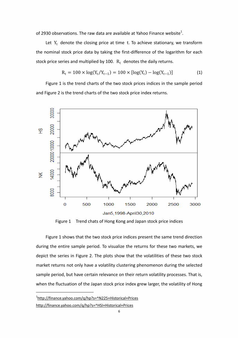
Figure 1 is the trend charts of the two stock prices indices in the sample period

and Figure 2 is the trend charts of the two stock price index returns.

Figure 1 Trend chats of Hong Kong and Japan stock price indices

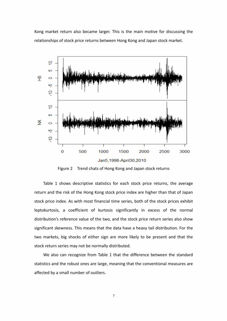
Figure 1 shows that the two stock price indices present the same trend direction

during the entire sample period. To visualize the returns for these two markets, we

depict the series in Figure 2. The plots show that the volatilities of these two stock

market returns not only have a volatility clustering phenomenon during the selected

sample period, but have certain relevance on their return volatility processes. That is,

when the fluctuation of the Japan stock price index grew larger, the volatility of Hong

1http://finance.yahoo.com/q/hp?s=^N225+Historical+Prices

http://finance.yahoo.com/q/hp?s=^HSI+Historical+Prices

7

Kong market return also became larger. This is the main motive for discussing the

relationships of stock price returns between Hong Kong and Japan stock market.

Figure 2 Trend chats of Hong Kong and Japan stock returns

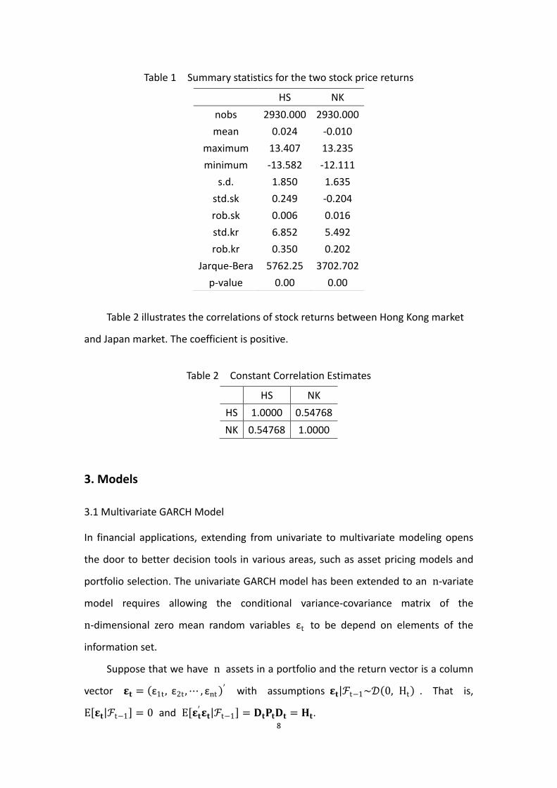
Table 1 shows descriptive statistics for each stock price returns, the average

return and the risk of the Hong Kong stock price index are higher than that of Japan

stock price index. As with most financial time series, both of the stock prices exhibit

leptokurtosis, a coefficient of kurtosis significantly in excess of the normal

distribution’s reference value of the two, and the stock price return series also show

significant skewness. This means that the data have a heavy tail distribution. For the

two markets, big shocks of either sign are more likely to be present and that the

stock return series may not be normally distributed.

We also can recognize from Table 1 that the difference between the standard

statistics and the robust ones are large, meaning that the conventional measures are

affected by a small number of outliers.

8

Table 1 Summary statistics for the two stock price returns

Table 2 illustrates the correlations of stock returns between Hong Kong market

and Japan market. The coefficient is positive.

Table 2 Constant Correlation Estimates

HS NK

HS 1.0000 0.54768

NK 0.54768 1.0000

3. Models

3.1 Multivariate GARCH Model

In financial applications, extending from univariate to multivariate modeling opens

the door to better decision tools in various areas, such as asset pricing models and

portfolio selection. The univariate GARCH model has been extended to an n-variate

model requires allowing the conditional variance-covariance matrix of the

n-dimensional zero mean random variables εt to be depend on elements of the

information set.

Suppose that we have n assets in a portfolio and the return vector is a column

vector 𝛆𝐭 = ε1t , ε2t , ⋯ , εnt ′ with assumptions 𝛆𝐭 ℱt−1~𝒟 0, Ht . That is,

E 𝛆𝐭 ℱt−1 = 0 and E 𝛆𝐭

′𝛆𝐭 ℱt−1 = 𝐃𝐭𝐏𝐭𝐃𝐭 = 𝐇𝐭.

HS NK

nobs 2930.000 2930.000

mean 0.024 -0.010

maximum 13.407 13.235

minimum -13.582 -12.111

s.d. 1.850 1.635

std.sk 0.249 -0.204

rob.sk 0.006 0.016

std.kr 6.852 5.492

rob.kr 0.350 0.202

Jarque-Bera 5762.25 3702.702

p-value 0.00 0.00

9

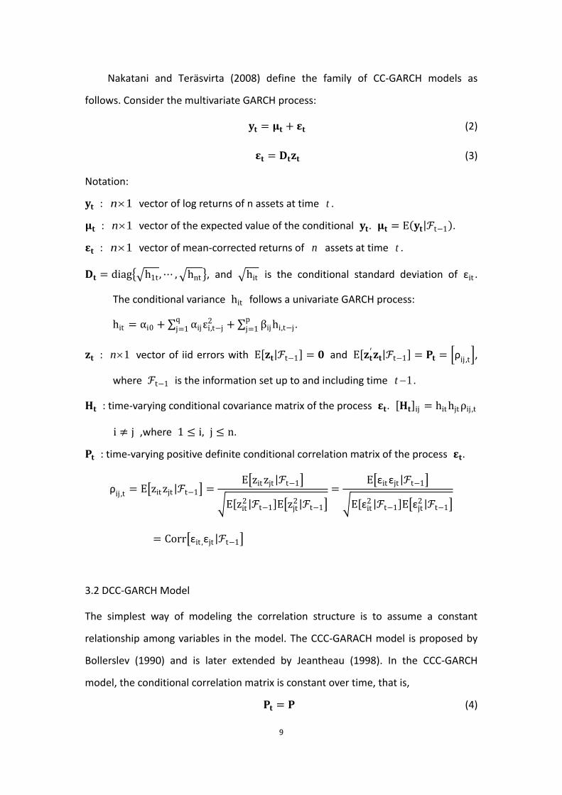
Nakatani and Teräsvirta (2008) define the family of CC-GARCH models as

follows. Consider the multivariate GARCH process:

𝐲𝐭 = 𝛍𝐭 + 𝛆𝐭 (2)

𝛆𝐭 = 𝐃𝐭𝐳𝐭 (3)

Notation:

𝐲𝐭 : 1n vector of log returns of n assets at time t .

𝛍𝐭 : 1n vector of the expected value of the conditional 𝐲𝐭. 𝛍𝐭 = E 𝐲𝐭 ℱt−1 .

𝛆𝐭 : 1n vector of mean-corrected returns of n assets at time t .

𝐃𝐭 = diag h1t , ⋯ , hnt , and hit is the conditional standard deviation of εit .

The conditional variance hit follows a univariate GARCH process:

hit = αi0 + αijεi,t−j2q

j=1 + βij hi,t−jpj=1 .

𝐳𝐭 : 1n vector of iid errors with E 𝐳𝐭 ℱt−1 = 𝟎 and E 𝐳𝐭

′𝐳𝐭 ℱt−1 = 𝐏𝐭 = ρij ,t ,

where ℱt−1 is the information set up to and including time 1t .

𝐇𝐭 : time-varying conditional covariance matrix of the process 𝛆𝐭. 𝐇𝐭 ij = hit hjtρij ,t

i ≠ j ,where 1 ≤ i, j ≤ n.

𝐏𝐭 : time-varying positive definite conditional correlation matrix of the process 𝛆𝐭.

ρij ,t = E zit zjt ℱt−1 =

E zit zjt ℱt−1

E zit2 ℱt−1

E zjt2 ℱt−1

=E εit εjt ℱt−1

E εit2 ℱt−1

E εjt2 ℱt−1

= Corr εit ,εjt ℱt−1

3.2 DCC-GARCH Model

The simplest way of modeling the correlation structure is to assume a constant

relationship among variables in the model. The CCC-GARACH model is proposed by

Bollerslev (1990) and is later extended by Jeantheau (1998). In the CCC-GARCH

model, the conditional correlation matrix is constant over time, that is,

𝐏𝐭 = 𝐏 (4)

10

However, the assumption of Bollerslev’s (1990) model that the conditional

correlations are constant over time may seem too restrictive in practice, and for this

reason many authors have proposed models of time-varying conditional correlations.

Thus, Engle (2002) and Tse and Tsui (2002) propose a generalization of Bollerslev’s

(1990) constant conditional correlation model by making the conditional correlation

matrix time-dependent. This type of model is called a dynamic conditional

correlation (DCC) model and it is one of the most popular CCC-GARCH models with

time-varying conditional correlations.

Engle (2002) applies GARCH-type dynamics in modeling the conditional

correlations. Its correlation structure is defined as follows:

𝐏𝐭 = 𝐐𝐭⨀𝐈𝐍 −1 2 𝐐𝐭 𝐐𝐭⨀𝐈𝐍

−1 2 (5)

𝐐𝐭 = 1 − α − β 𝐐 + α𝐳𝐭−𝟏𝐳𝐭−𝟏′ + β𝐐𝐭−𝟏 (6)

where

α + β < 1 𝑎𝑛𝑑 𝛼 > 0, 𝛽 > 0

Notation:

IN = E 𝐳𝐭′𝐳𝐭

⨀: the Hadmard or element wise product of the two conformable matrices.

𝐐: a sample covariance matrix of 𝐳𝐭.

In this formulation, the correlation process is driven by two parameters,

α and β. This is one of the advantages of the DCC-GARCH model in the sense that the

number of parameters to be estimated for conditional correlations does not depend

on the number of variables in the model. With this property, one can alleviate the

computational burden and yet obtain large-dimensional correlations. But the simple

structure of the DCC-GARCH parameterizations may be seen as a weakness because

all the correlation processes are assumed to have the same dynamic behavior.

3.3 Model Building

In this paper, we use the bivariate DCC-GARCH model to discuss the relationships

between Japan stock market and Hong Kong stock market, and impact on returns of

11

the two markets. The simplest but often very useful DCC-GARCH process is of course

the DCC-GARCH (1, 1) process. The constructions of the model are as follows:

RHSt = ϕ0 + ϕ1kRHSt−kpk=1 + ϕ2kRNKt−k

pk=1 + ε1,t (7)

RNKt = φ0 + φ1kRHSt−kpk=1 + φ2kRNKt−k + ε2,t

pk=1 (8)

h11,t = α10 + α11ε1,t−12 + β11h11,t−1 (9)

h22,t = α20 + α21ε2,t−12 + β21h22,t−1 (10)

𝐏𝐭 = 𝐐𝐭⨀𝐈𝐍 −1 2 𝐐𝐭 𝐐𝐭⨀𝐈𝐍

−1 2 (11)

𝐐𝐭 = 1 − α − β 𝐐 + α𝐳𝐭−𝟏𝐳𝐭−𝟏′ + β𝐐𝐭−𝟏 (12)

4. Analysis and Results

4.1 Estimation of DCC-GARCH Model

In this part, we describe how the parameters of a DCC-GARCH model may be

determined. The likelihood function for 𝛆𝐭 = 𝐃𝐭𝐳𝐭 is

ℒ 𝛉 = 1

2π 𝐇𝐭 Nt=1 exp −

1

2𝛆𝐭′𝐇𝐭

−𝟏𝛆𝐭 (13)

The log-likelihood function of the DCC-GARCH model at time t is in general

given by

ℓ 𝛉 = ln L 𝛉 = −N

2ln 2π −

1

2ln 𝐇𝐭 −

1

2𝛆𝐭′𝐇t

−1𝛆𝐭 (14)

= −N

2ln 2π −

1

2ln 𝐃𝐭𝐏𝐭𝐃𝐭 −

1

2𝛆𝐭′𝐃t

−1𝐏𝐭−𝟏𝐃𝐭

−𝟏𝛆𝐭

The log-likelihood function can be decomposed into two parts, namely the

volatility component and the correlation component. The volatility component at

time t is given by

ℓv,t 𝛚 = −N

2ln 2π −

1

2ln 𝐕𝐭 −

1

2𝛆𝐭′𝐕t

−1𝛆𝐭 (15)

where Vt = Dt2, and the correlation component at time t is

ℓc,t 𝛚,𝛗 = −1

2ln 𝐏𝐭 −

1

2𝐳𝐭′𝐏𝐭

−𝟏𝐳𝐭 +1

2𝐳𝐭′𝐳𝐭 (16)

By applying this decomposition, the estimation of a DCC-GARCH model can be

12

carried out in two steps. First, maximize (15) with respect to 𝛚 which denotes the

parameters in the volatility component. Second, maximize (16) with respect to 𝛗

which denotes the parameters in the correlation component, given the estimates

from the preceding step. It is worth mentioning that the constraints on α and β

must be satisfied throughout the iterations because otherwise 𝐐𝐭 may become an

explosive sequence.

4.2 Parameter Estimation

The equations (7) and (8) can be written as:

RHSt

RNKt =

ϕ0

φ0 +

ϕ11 ⋯ ϕ2p

φ11 ⋯ φ2p

RHSt−1

⋮RNKt−p

+ ε1,t

ε2,t (17)

This is p-th order vector autoregressive model. We choose the value of p by

using some model selection criteria, such as Akaike Information Criterion (AIC),

Hanna-Quinn Information Criterion (HQ) and Schwarz Information Criterion (SC). All

of these selection criteria are not the same when they are used in the univariate

model.

AIC n = ln det n ~u +

2

TnK2 (18)

HQ n = ln det n ~u +

2ln ln T

TnK2 (19)

SC n = ln det n ~u +

ln T

TnK2 (20)

where n ~u = T−1 u tu t

′,′Tt=1 and n∗ is the total number of the parameters in

each equation and n assigns the lag order.

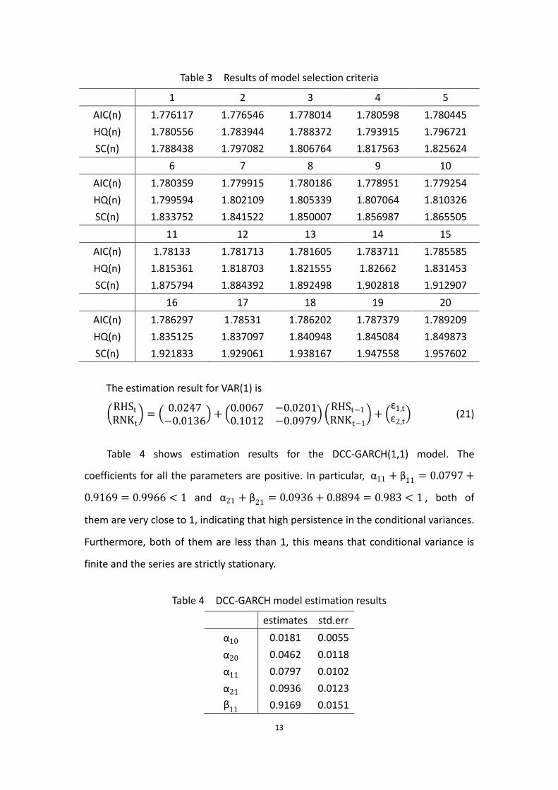
In table 3, from fitted models with p = 1,2, ⋯ ,20, we choose the value of p

which has the minimal selection criteria; therefore, p = 1.

13

Table 3 Results of model selection criteria

1 2 3 4 5

AIC(n) 1.776117 1.776546 1.778014 1.780598 1.780445

HQ(n) 1.780556 1.783944 1.788372 1.793915 1.796721

SC(n) 1.788438 1.797082 1.806764 1.817563 1.825624

6 7 8 9 10

AIC(n) 1.780359 1.779915 1.780186 1.778951 1.779254

HQ(n) 1.799594 1.802109 1.805339 1.807064 1.810326

SC(n) 1.833752 1.841522 1.850007 1.856987 1.865505

11 12 13 14 15

AIC(n) 1.78133 1.781713 1.781605 1.783711 1.785585

HQ(n) 1.815361 1.818703 1.821555 1.82662 1.831453

SC(n) 1.875794 1.884392 1.892498 1.902818 1.912907

16 17 18 19 20

AIC(n) 1.786297 1.78531 1.786202 1.787379 1.789209

HQ(n) 1.835125 1.837097 1.840948 1.845084 1.849873

SC(n) 1.921833 1.929061 1.938167 1.947558 1.957602

The estimation result for VAR(1) is

RHSt

RNKt =

0.0247−0.0136

+ 0.0067 −0.02010.1012 −0.0979

RHSt−1

RNKt−1 +

ε1,t

ε2,t (21)

Table 4 shows estimation results for the DCC-GARCH(1,1) model. The

coefficients for all the parameters are positive. In particular, α11 + β11 = 0.0797 +

0.9169 = 0.9966 < 1 and α21 + β21 = 0.0936 + 0.8894 = 0.983 < 1 , both of

them are very close to 1, indicating that high persistence in the conditional variances.

Furthermore, both of them are less than 1, this means that conditional variance is

finite and the series are strictly stationary.

Table 4 DCC-GARCH model estimation results

estimates std.err

α10 0.0181 0.0055

α20 0.0462 0.0118

α11 0.0797 0.0102

α21 0.0936 0.0123

β11 0.9169 0.0151

14

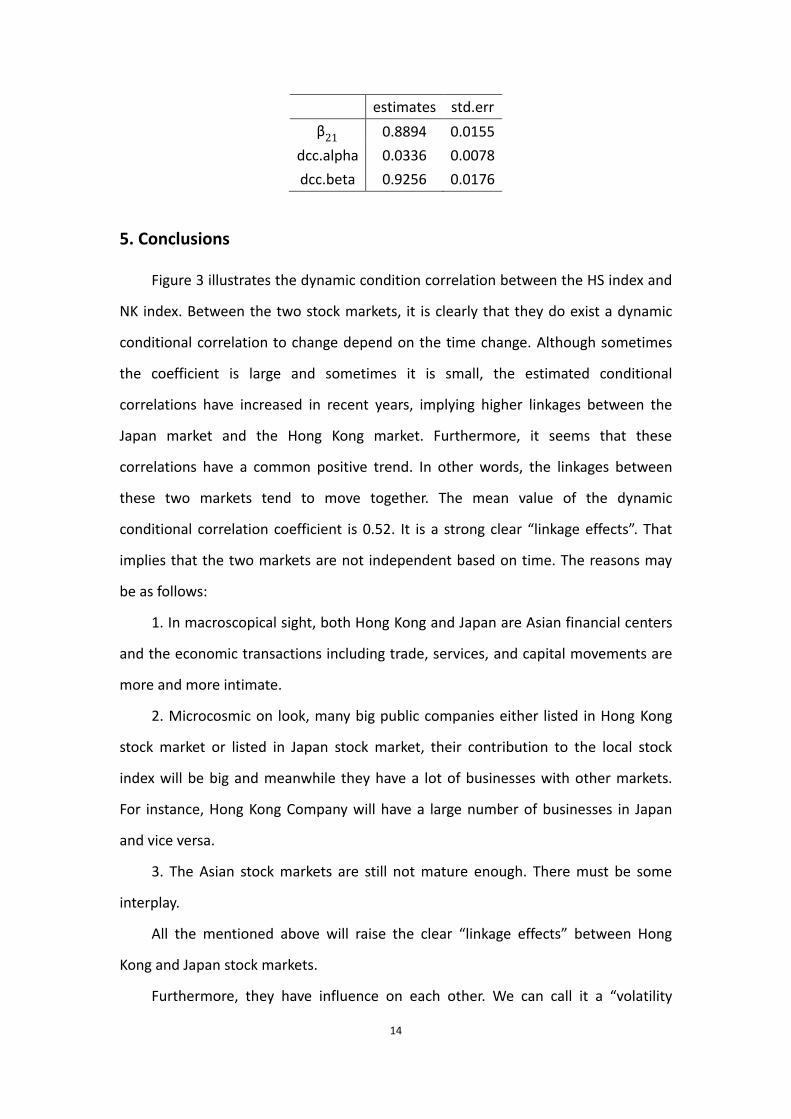
estimates std.err

β21 0.8894 0.0155

dcc.alpha 0.0336 0.0078

dcc.beta 0.9256 0.0176

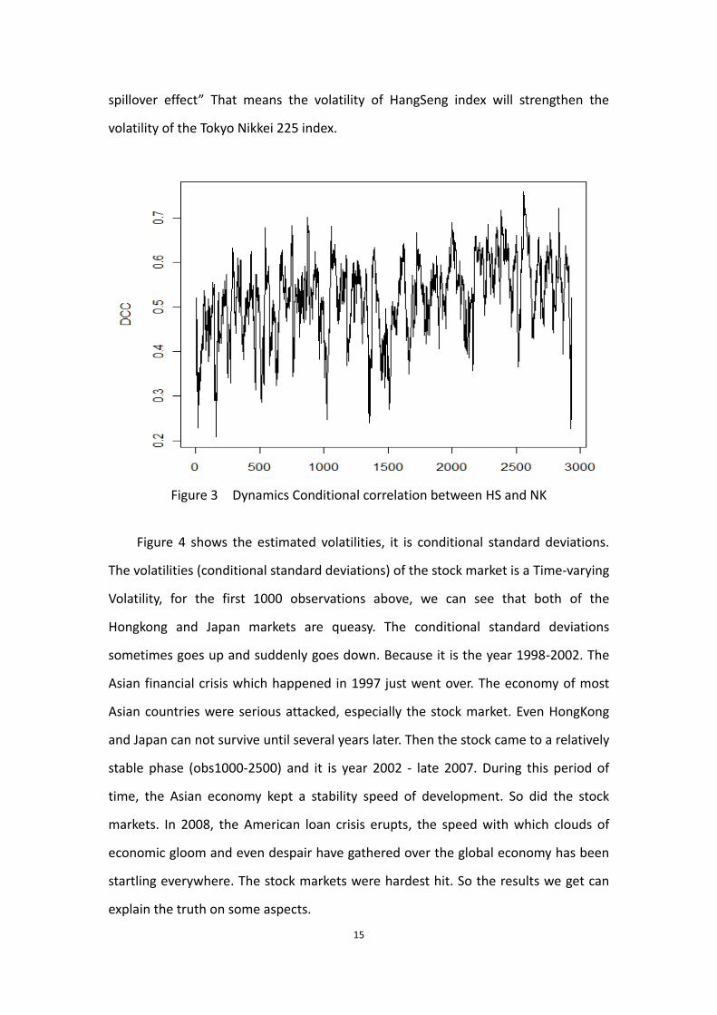
5. Conclusions

Figure 3 illustrates the dynamic condition correlation between the HS index and

NK index. Between the two stock markets, it is clearly that they do exist a dynamic

conditional correlation to change depend on the time change. Although sometimes

the coefficient is large and sometimes it is small, the estimated conditional

correlations have increased in recent years, implying higher linkages between the

Japan market and the Hong Kong market. Furthermore, it seems that these

correlations have a common positive trend. In other words, the linkages between

these two markets tend to move together. The mean value of the dynamic

conditional correlation coefficient is 0.52. It is a strong clear “linkage effects”. That

implies that the two markets are not independent based on time. The reasons may

be as follows:

1. In macroscopical sight, both Hong Kong and Japan are Asian financial centers

and the economic transactions including trade, services, and capital movements are

more and more intimate.

2. Microcosmic on look, many big public companies either listed in Hong Kong

stock market or listed in Japan stock market, their contribution to the local stock

index will be big and meanwhile they have a lot of businesses with other markets.

For instance, Hong Kong Company will have a large number of businesses in Japan

and vice versa.

3. The Asian stock markets are still not mature enough. There must be some

interplay.

All the mentioned above will raise the clear “linkage effects” between Hong

Kong and Japan stock markets.

Furthermore, they have influence on each other. We can call it a “volatility

15

spillover effect” That means the volatility of HangSeng index will strengthen the

volatility of the Tokyo Nikkei 225 index.

Figure 3 Dynamics Conditional correlation between HS and NK

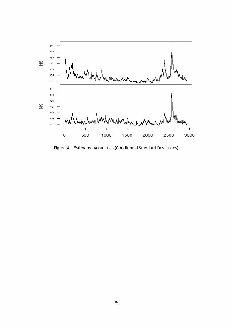
Figure 4 shows the estimated volatilities, it is conditional standard deviations.

The volatilities (conditional standard deviations) of the stock market is a Time-varying

Volatility, for the first 1000 observations above, we can see that both of the

Hongkong and Japan markets are queasy. The conditional standard deviations

sometimes goes up and suddenly goes down. Because it is the year 1998-2002. The

Asian financial crisis which happened in 1997 just went over. The economy of most

Asian countries were serious attacked, especially the stock market. Even HongKong

and Japan can not survive until several years later. Then the stock came to a relatively

stable phase (obs1000-2500) and it is year 2002 - late 2007. During this period of

time, the Asian economy kept a stability speed of development. So did the stock

markets. In 2008, the American loan crisis erupts, the speed with which clouds of

economic gloom and even despair have gathered over the global economy has been

startling everywhere. The stock markets were hardest hit. So the results we get can

explain the truth on some aspects.

16

Figure 4 Estimated Volatilities (Conditional Standard Deviations)

17

References

Bollerslev Tim. (1986). Generalized autoregressive conditional heteroskedasticity.

Journal of Econometrics, 31(3), pp.307-327.

Bollerslev Tim. (1987). A Conditional Heteroskedasticity Time Series Model for

Speculative Prices and Rates of Return. The Review of Economics and Statistics,

69(3), pp.542–547.

Bollerslev Tim, Engle Robert F. and Jeffrey M. Wooldridge. (1988). A Capital Asset

Pricing Model with Time-varying Covariances. The Journal of Political Economy,

96(1), pp.116-131.

Bollerslev Tim. (1990). Modeling the Coherence in Short-Run Nominal Exchange

Rates: A Multivariate Generalized Arch Model. The Review of Economics and

Statistics, 72(3), pp.498-505.

Billio Monica, Caporin Massimiliano and Gobbo Michele. (2003). Block Dynamic

Conditional Correlation Multivariate GARCH Model. Greta Working Paper,

No.03.03.

Balázs Égerta and Evžen Kočenda. (2007). Time-Varying Comovements in

Developed and Emerging European Stock Markets: Evidence from Intraday Data.

William Davidson Institute Working Paper, No.861.

Cappiello Lorenzo, Engle Robert F., and Sheppard Kevin. (2006). Asymmetric

Dynamics in the Correlations of Global Equity and Bond Returns. Journal of

Financial Econometrics, 4(4), pp.537-572.

Colm Kearney and Valerio Poti. (2003). DCC-GARCH Modeling of Market and

Firm-Level Correlation Dynamics in the Dow Jones Eurostoxx 50 Index. Paper

submitted to the European Finance Association Conference, Edinburgh, August

2003.

Engle Robert F.. (1982). Autogressive Conditional Heteroskedasticity with

Estimates of the Variance of United Kingdom Inflation. Econometric, 50(4),

pp.987-1008.

Engle Robert F. and Kroner Kenneth F.. (1995). Multivariate Simultaneous

18

Generalized ARCH. Econometric Theory, 11(1), pp.122-150.

Engle Robert F. and Sheppard Kevin. (2001). Theoretical and Empirical Properties

of Dynamic Conditional Correlation Multivariate GARCH. UCSD Working Paper

NO.2001-15.

Engle Robert F.. (2002). Dynamic Conditional Correlation - A Simple Class of

Multivariate GARCH Models. Journal of Business and Economic Statistics, 20(3),

pp.339-350.

Hamilto, J.D. (1994). Time series analysis, Princeton University Press, Princeton

NJ.

He Changli and Teräsvirta Timo. (2004). An Extended Constant Conditional

Correlation Garch Model and its Fourth-Moment Structure. Econometric Theory,

20, pp.904-926.

Ljung G.M. and Box G.E.P.. (1978). On a Measure of Lack of Fit in Time Series

Models. Biometrika, 65(2), pp.297-303.

Mohamed El Hedi Arouri, Fredj Jawadi and Duc Khuong Nguyen. (2008),

International Stock Return Linkages: Evidence from Latin American Markets.

European Journal of Economics, Finance and Administrative Sciences, 11,

pp.57-65.

Nelson Daniel B.. (1991). Conditional Heteroskedasticity in Asset Returns: a New

Approach. Econometrica, 59(2), pp.347-370.

Nakatani Tomoaki and Teräsvirta Timo. (2009). Testing for Volatility Interactions

in the Constant Conditional Correlation GARCH Model. Econometrics Journal,

12(1), pp.147-163.

Nathaniel Frank, Brenda González-Hermosillo and Heiko Hesse. (2008).

Transmission of Liquidity Shocks: Evidence from the 2007 Subprime Crisis.

International Monetary Fund Working Paper, No.200.

Sheppard Kevin. (2001). Multi-step Estimation of Multivariate GARCH Models.

Second International ICSC Symposium on Advanced Computing Financial Markets,

Paper No.1744-137.

Silvennoinen Annastiina and Teräsvirta Timo. (2005). Multivariate Autoregressive

19

Conditional Heteroskedasticity with Smooth Transitions in Conditional

Correlations. SSE/EFI Working Paper Series in Economics and Finance, No.577,

Stockholm School of Economics.

Therese Peters. (2008). Forecasting the covariance matrix with the DCC GARCH

model. Stockholm University, Examensarbete, 2008:4.