Embed Size (px)
Citation preview
Modeling Market Sentiment and Conditional Distribution of
Stock Index Returns under GARCH Process
A final project submitted to the faculty of Claremont Graduate University in partial fulfillment of
the requirements for the degree of Doctor of Philosophy in Economics
by
Ali Arik
Claremont Graduate University
2011
© Copyright Ali Arik, 2011
All rights reserved.

Abstract
(Modeling Market Sentiment and Conditional Distribution of Stock Index Returns
under GARCH Process)
by
Ali Arik
Claremont Graduate University: 2011
In finance, one of the greatest challenges is to measure investor sentiment correctly. A
shortcoming of previous studies has been their failure to find an appropriate methodology which
would define market sentiment correctly and use stock volatility to measure a direct relationship
between sentiment and expected returns. Using survey-based measures of both individual and
institutional investor sentiment, along with a set of macroeconomic variables, I employ a
generalized autoregressive conditional heteroscedasticity specification, which employs not only
the conditional volatility but also implied volatility (VIX) in the mean equation to test the impact
of investor sentiment on stock returns. First, I find support for a negative relation between stock
returns and implied volatility. Second, I find a positive and statistically significant relationship
between changes in the sentiment Bull Ratio of both institutional and individual investors and
S&P 500 excess returns in the following month. The estimation results also suggest that the
opinions of institutional investors seem to relate to market data better than those of individual
investors. In behavioral models, it is believed that investors' widespread optimism and pessimism
can cause prices to deviate from their fundamental values, leading to temporary price corrections
in the form of mean-reverting behavior when those expectations are not met. Using periodic
realized market returns as anchors, I find a positive (negative) insignificant (significant)
relationship between daily index returns and bullish (bearish) sentiment. These effects are
stronger when the state of implied volatility is controlled as low, moderate, and high state.

1
Table of Contents
Chapter I .......................................................................................................................................... 2
Investigating the Relationship between Implied Volatility and Stock Returns .............................. 2
I. Introduction .......................................................................................................................... 2
II. Understanding VIX ................................................................................................................ 3
III. VIX as measuring Fear .......................................................................................................... 5
IV. VIX under different Regimes ................................................................................................ 8
V. Chapter Conclusion .............................................................................................................. 9
Chapter II ....................................................................................................................................... 10
Measuring Market Sentiment and Stock Index Returns ............................................................... 10
I. Literature Review ............................................................................................................... 10
II. Methodology for Measuring Investor Sentiment .............................................................. 13
III. Methodology for Measuring Index Returns ....................................................................... 17
IV. Model ................................................................................................................................. 18
V. Data, Descriptive Statistics, and Estimation Results .......................................................... 28
VI. Chapter Conclusion ............................................................................................................ 44
Chapter III ...................................................................................................................................... 45
Effects of Investor Sentiment and Implied Volatility on Daily Returns ........................................ 45
I. Introduction ........................................................................................................................ 45
II. Methodology ...................................................................................................................... 46
III. Empirical Results ................................................................................................................ 56
IV. Chapter Conclusion ............................................................................................................ 61
V. Final Conclusion .................................................................................................................. 62
2
Chapter I
Investigating the Relationship between Implied Volatility
and Stock Returns
I. Introduction
Since Markowitz (1952, 1959), who laid the groundwork for the Capital Asset Pricing
Model (CAPM), forecasting volatility has become one of the great success stories in finance.
Markowitz formulates the theory of optimal portfolio selection problem in terms of expected
return and risk and argues that investors would optimally hold a mean-variance effect portfolio, a
portfolio with the highest expected return for a given level of variance. A stock that is volatile is
also considered higher risk because its performance may change quickly in either direction at any
time. However, volatility is only one indicator of risk affecting a stock. Investors pay attention to
volatility not because it is perceived as a mere measure of risk, but because they worry about
unusual levels of excessive volatility, especially when observed fluctuations in a stock price do
not seem to be accommodated by any related news about the firm's fundamentals. If this is the
case, the stock price no longer might play its role as a signal about the true intrinsic value of a
firm, Karolyi (2001). After Black and Scholes (1973) option pricing model, the use of implied
volatility (versus historical volatility) in forecasting expected returns has become popular among
researchers. For instance, Ederington and Guan (2002) find that most implied standard deviations
averages calculated from several options for the S&P 500 futures options market forecast
expected volatility better than naive time series models, concluding that "implied volatility has
strong predictive power and generally subsumes the information in historical volatility" (p.29).

3
II. Understanding VIX
Because many investors hold more than one stock, it is more suitable to measure or pay
attention to the volatility of an index. The VIX index was introduced by R. Whaley in 1993 for
S&P 100 index. In 2003, CBOE together with Goldman Sachs, updated the VIX calculation
based on S&P 500 index by averaging the weighted prices of the index's vanilla puts and calls
(that are not exotic) over a wide range of strike prices.1 Conventional wisdom is that VIX tends
to trend in the very short-term, mean reverting over the short-intermediate term, and moves in
cycles over the long-term. Examination of Figure 1 over the sample period from 2001:01 -
2011:02 reveals that VIX is low and stable between 2003 and 2008, after the dot-com crisis and
before the financial meltdown of 2008. During the dot-com crisis, VIX usually remained
between 20 and 40. Also observe that right around the time of the housing crisis, it remained
mostly above 20 as well as reaching its all time high level of 80. Since May 2010, VIX has come
down to its low 20 level again as the economy gets itself out of recession.
1 VIX futures and options have become tradable assets in Exchange history. VIX represents the expected market volatility over the next 30 calendar days. It is the volatility of a variance swap1. For example, VIX 25 means that the market expects an annualized change of 25 percent in volatility over the next 30 days. This roughly corresponds to monthly 7.21 percent
, means that the Index options are priced with the assumption of 68 percent likelihood (plus-minus one
standard deviation) that the magnitude of the S&P 500 index 30-day return will be less than 7.21 percent (up or down).
0
10
20
30
40
50
60
70
80
90 Vix
Figure 1
4
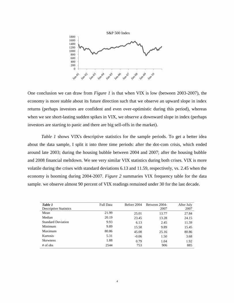
One conclusion we can draw from Figure 1 is that when VIX is low (between 2003-2007), the
economy is more stable about its future direction such that we observe an upward slope in index
returns (perhaps investors are confident and even over-optimistic during this period), whereas
when we see short-lasting sudden spikes in VIX, we observe a downward slope in index (perhaps
investors are starting to panic and there are big sell-offs in the market).
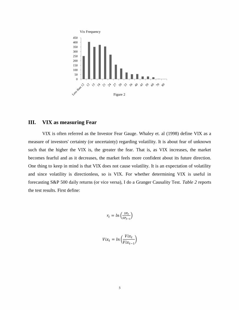
Table 1 shows VIX's descriptive statistics for the sample periods. To get a better idea
about the data sample, I split it into three time periods: after the dot-com crisis, which ended
around late 2003; during the housing bubble between 2004 and 2007; after the housing bubble
and 2008 financial meltdown. We see very similar VIX statistics during both crises. VIX is more
volatile during the crises with standard deviations 6.13 and 11.59, respectively, vs. 2.45 when the
economy is booming during 2004-2007. Figure 2 summaries VIX frequency table for the data
sample. we observe almost 90 percent of VIX readings remained under 30 for the last decade.
Table 1 Descriptive Statistics
Full Data Before 2004 Between 2004-2007
After July 2007
Mean 21.99 25.01 13.77 27.84
Median 20.19 23.45 13.28 24.15
Standard Deviation 9.93 6.13 2.45 11.59 Minimum 9.89 15.58 9.89 15.45
Maximum 80.86 45.08 25.16 80.86
Kurtosis 5.31 -0.06 1.50 3.68
Skewness 1.88 0.79 1.04 1.92
# of obs 2544 753 906 885
0
200
400
600
800
1000
1200
1400
1600
1800
S&P 500 Index
5
III. VIX as measuring Fear
VIX is often referred as the Investor Fear Gauge. Whaley et. al (1998) define VIX as a
measure of investors' certainty (or uncertainty) regarding volatility. It is about fear of unknown
such that the higher the VIX is, the greater the fear. That is, as VIX increases, the market
becomes fearful and as it decreases, the market feels more confident about its future direction.
One thing to keep in mind is that VIX does not cause volatility. It is an expectation of volatility
and since volatility is directionless, so is VIX. For whether determining VIX is useful in
forecasting S&P 500 daily returns (or vice versa), I do a Granger Causality Test. Table 2 reports
the test results. First define:
0
50
100
150
200
250
300
350
400
450
Vix Frequency
Figure 2
6
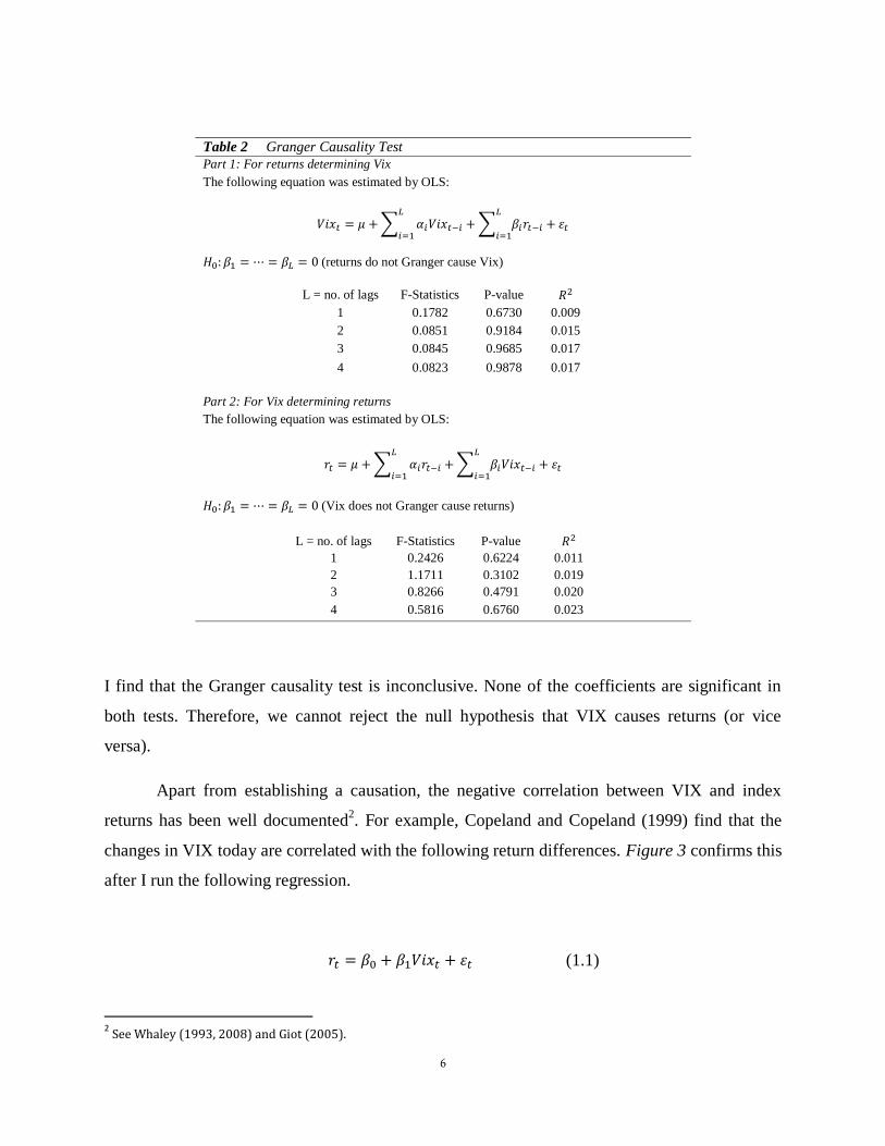
Table 2 Granger Causality Test
Part 1: For returns determining Vix
The following equation was estimated by OLS:
(returns do not Granger cause Vix)
L = no. of lags F-Statistics P-value
1 0.1782 0.6730 0.009
2 0.0851 0.9184 0.015
3 0.0845 0.9685 0.017
4 0.0823 0.9878 0.017
Part 2: For Vix determining returns
The following equation was estimated by OLS:
(Vix does not Granger cause returns)
L = no. of lags F-Statistics P-value
1 0.2426 0.6224 0.011
2 1.1711 0.3102 0.019
3 0.8266 0.4791 0.020
4 0.5816 0.6760 0.023
I find that the Granger causality test is inconclusive. None of the coefficients are significant in
both tests. Therefore, we cannot reject the null hypothesis that VIX causes returns (or vice
versa).
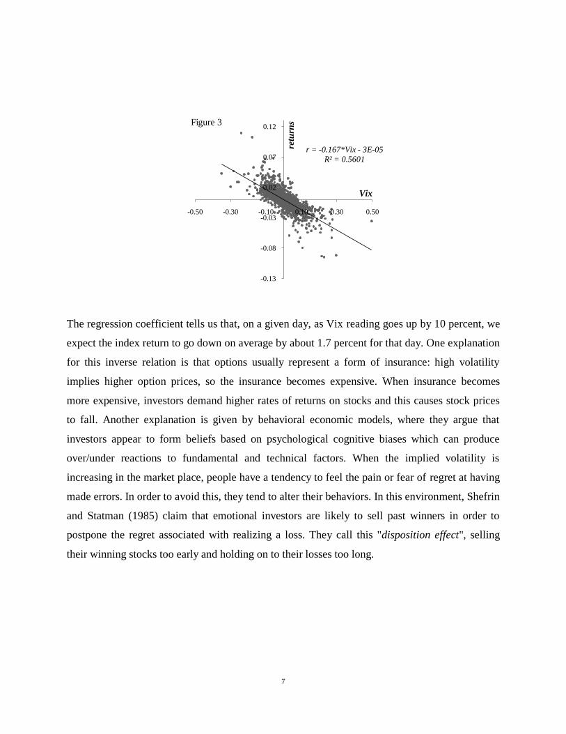
Apart from establishing a causation, the negative correlation between VIX and index
returns has been well documented2. For example, Copeland and Copeland (1999) find that the
changes in VIX today are correlated with the following return differences. Figure 3 confirms this
after I run the following regression.
(1.1)
2 See Whaley (1993, 2008) and Giot (2005).
7
The regression coefficient tells us that, on a given day, as Vix reading goes up by 10 percent, we
expect the index return to go down on average by about 1.7 percent for that day. One explanation
for this inverse relation is that options usually represent a form of insurance: high volatility
implies higher option prices, so the insurance becomes expensive. When insurance becomes
more expensive, investors demand higher rates of returns on stocks and this causes stock prices
to fall. Another explanation is given by behavioral economic models, where they argue that
investors appear to form beliefs based on psychological cognitive biases which can produce
over/under reactions to fundamental and technical factors. When the implied volatility is
increasing in the market place, people have a tendency to feel the pain or fear of regret at having
made errors. In order to avoid this, they tend to alter their behaviors. In this environment, Shefrin
and Statman (1985) claim that emotional investors are likely to sell past winners in order to
postpone the regret associated with realizing a loss. They call this "disposition effect", selling
their winning stocks too early and holding on to their losses too long.
r = -0.167*Vix - 3E-05
R² = 0.5601
-0.13
-0.08
-0.03
0.02
0.07
0.12
-0.50 -0.30 -0.10 0.10 0.30 0.50
retu
rns
Vix
Figure 3

8
IV. VIX under different Regimes
In this section, I investigate how sensitive the S&P 500 index returns are under different
VIX readings. I first split VIX data into three categories: low, moderate, and high. The
distribution of VIX, not reported here, has a mean of roughly 22 for the data sample. So I define
a moderate regime as plus/minus half standard deviation from its mean, which corresponds to a
range between 17.02 and 26.95. There are about 894 low regime, 1105 moderate regime, and 544
high regime observations for the sample period, corresponding 35%, 44%, and 21%, respectively
indicating that it skewed left. The claim is that the slope of the regression line in Equation (1.1)
should be steeper in high volatility state than it is in low or moderate state. The following
regression is run to test this.
(1.2)
For each regime i, if . .
As claimed, Figure 4 shows that stock index returns are more sensitive under high implied
volatility state. DeBondt amd Thaler (1985) argue that investors are subject to waves of
r = -0.0943Vix + 0.0005
R² = 0.6027
-0.1
-0.05
0
0.05
0.1
-0.5 0 0.5
Ret
urn
s
Vix
Low
r = -0.142Vix + 0.0004
R² = 0.6159
-0.1
-0.05
0
0.05
0.1
-0.5 0 0.5
Ret
urn
s
Vix
Moderate
Figure 4
r = -0.2519Vix - 0.0006
R² = 0.6503
-0.1
-0.05
0
0.05
0.1
-0.5 0 0.5
Ret
un
s
Vix
High

9
optimisim and pessimism of herding bias. Investors who communicate regularly tend to think
and act similarly, perhaps they avoid being wrong in the group. In this tendency, they adopt the
opinions and follow the behavior of the majority to feel safer and to avoid conflict. When VIX
gets high, there is a greater panic and fear in the market place, which leads investors to sell off
their holdings quicker than they would normally do. As a result, index returns drop sharply. We
can apply the same logic to low VIX state, where investors do not expect big swings in stock
prices and are more confident and optimistic about the direction of the market. When VIX goes
up in this environment, they may not see it as a treat but instead as a temporary price correction.
Therefore, they may choose to ignore it and react less by holding onto their positions longer.
V. Chapter Conclusion
In this chapter, I briefly argue that there is a strong relationship between implied
volatility and index returns. VIX is believed to be a measure of investors' certainty regarding
volatility. High volatility implies price turbulences (usually negative sharp drops in prices),
whereas low volatility implies price stability (usually price-rallies and bubbles). In the next
chapter, using survey-based data, I employ a generalized autoregressive conditional
heteroscedasticity specification, where implied volatility (VIX) is exogenously added in the
mean equation to test the impact of investor sentiment on stock returns.

10
Chapter II
Measuring Market Sentiment and Stock Index Returns
I. Literature Review
I.1. Earlier Studies
Over the years, numerous studies have been carried out on understanding how investors
trade in the stock market. For many economists during the early period of the twentieth century,
financial markets were still regarded as mere casinos. In standard finance, the expected utility
theory (which focuses on the level of wealth) offers a representation of truly rational behavior
under certainty. Using consumption discount models, Lucas (1978) claims that all investors have
rational expectations and stock prices do fully reflect all available information.3 He argues that if
we can forecast agents' future consumption, rational asset prices may have a forecastable element
related to consumption. However, Grossman and Shiller (1981) found that consumption discount
models do not work very well unless the coefficient of relative risk aversion is set very high.
In contrast to the expected utility theory, Kahneman and Tversky (1979, 1992) offer the
prospect theory, in which utility is defined over gains and losses (i.e. returns), relevant to a
reference point rather than levels of wealth. They document behavioral systematic cognitive
biases that are very common in human decision-making under uncertainty. They claim that
people do not obey the normal axioms of the finance theory (expected utility; risk aversion
problem; Bayesian updating; decision under uncertainty; and rational expectations) and they
claim Bayes’ rule is not an apt characterization of how individuals actually respond to new data.
―…perhaps the most robust finding in the psychology of judgment is that people are
overconfident…‖ (Kahneman and Tversky 1982).
Behavioral economists claim that understanding the behaviors of market participants is
the key to understanding the market. These studies give psychological evidence explaining why
3 This is the neoclassical version of the Efficient Market Hypothesis.

11
and how people make systematic errors in the way they think and claim that economists have
ignored these biases in prior studies because they thought they would disappear when the stakes
are high (LeRoy 1989). But today we see evidence that these biases are too important to ignore.4
For example, representative bias is believed to lead investors to overreact to news while
conservative bias leads investors to underreact to news.5
One of the major criticisms of behavioral finance is that people can find a story to fit the
facts. LeRoy (1989) states that behavioral models are more successful in providing ―after-the-
fact‖ explanations for observed behavior than in generating testable predictions. Malkiel (2003)
gives a good summary of why people should be skeptical of empirical results reported in
behavioral finance literature. He believes that apparent patterns are extremely rare or too
unstable to guarantee consistently superior investment results.
In many behavioral models inspired by DeLong, Shleifer, Summers, and Waldmann
(DSSW (1990) hereafter), investors are of two types: professional investors who are sentiment-
free and inexperienced investors who are prone to sentiment. In the effort of measuring investor
sentiment and quantifying its effect, researchers mainly focused on Noise Trading theory, where
individual (inexperienced) investors are blamed for creating excessive market volatility (noise).
For example, according to Black (1986), the price of a stock reflects two things: information
(that is observable and professional traders trade on) and noise (that is unobservable and the
individual traders trade on). He claims that noise is the major reason for the use of decision rules
that seem to violate the normal axioms of the finance theory. Shleifer and Summers (1990) argue
that noise (rather than information) drives market participants’ decisions in financial markets.
DSSW (1990a, b) claim that noise traders falsely believe that they have unique information
about the future price of a risky asset. Daniel et al. (1998) define noise trading as ―variability in
prices arising from unpredictable trading that seems unrelated to valid information‖.
By definition, inexperienced traders have different beliefs from other professional
4 See Barberis and Thaler (2003) “Survey of a Behavioral Finance” for details. Several papers document such behavioral biases as overconfidence Daniel, Hirshleifer, and Subrahmanymean (1998); Barber and Odean (2001); Gervais and Odean (2001), as overreaction DeBondt and Thaler (1985), as loss aversion Kahneman and Tversky (1979); Shefrin and Statman (1985); Odean 1998, as herding Huberman and Regev (2001), as mental accounting Kahneman and Tversky (1981), and as regret.
5 Griffin and Tversky (1992) state that in revising their forecast, people focus too much on the strength of the evidence and too little on its weight, relative to a rational Bayesian. Barberis, Shleifer, and Vishny (1998) explain representativeness as people’s belief that they see patterns in random sequences.

12
investors, usually resulting from differences in processing information. One claim is that
individual traders may lack the ability to distinguish noise from information; they think they are
trading on information and do not know that they are trading on noise.
I.2. Recent Studies
In the literature, investor sentiment is defined as the general attitude towards the
accumulation of a variety of fundamental and technical factors and takes three forms: bullish,
bearish, and uncertain. Brown and Cliff (2004, 2005) suggest that stock market return and
investor sentiment may act in a system. They employ two types of sentiment measures: one is
direct measures from surveys, and the other is indirect measures from various market data such
as market performance variables, derivative variables, and other sentiment measures such as
closed-end fund discount rate, net purchases of mutual funds, proportion of fund assets held in
cash, and number of IPOs. They find strong evidence that their sentiment measures co-move
with the market in the long run (2-3 years). However, they find little evidence that sentiment has
predictive power for near-term future stock returns.
Baker and Wurgler (2004, 2006, 2007) discuss cross-sectional differences in the time
series of the stock returns. They claim that sentiment may differ across stocks and arbitrage
possibilities may be different from one stock to another. They find evidence that investor
sentiment affects the cross-section of stock returns and that the impacts are most profound on the
stocks whose valuation is highly subjective and difficult to arbitrage. They suggest that the
stocks most sensitive to shifts in investor sentiment are those companies that are younger,
smaller, unprofitable, non-dividend paying, distressed, have extreme growth potential, and that
have higher betas. These stocks will exhibit high sentiment beta.
Fisher and Statman (2000) were among the first to use survey-based measures of investor
sentiment. They used three groups of investors: small investors (who are individuals taking
American Association Individual Investors (AAII) surveys), semiprofessional investors (who are
newsletter writers), and large investors (who are the institutions and Wall Street strategists).
Using level of sentiment, they find that the sentiments of the three groups do not move together.
Although both small investors and the semiprofessional investors are prone to be influenced by
13
past returns, large investors are more careful and are not easily influenced by the past market
price movements.
Verma and Soydemir (2009) employ survey-based data. Unlike the previous studies
which usually treat sentiment as fully irrational, they focus on both rational and irrational
components of investor sentiment. They use two surveys’ data: individual investor survey from
AAII and institutional investor survey from Investor Intelligence (II). They regress both these
surveys on various rational factors including classical Fama-French factors and then, they define
the fitted values from these regressions as the rational component of sentiment and the residuals
as the irrational component of sentiment. Consistent with Brown and Cliff (2004), they find
weak evidence between sentiment and market return in the short run but stronger evidence in the
case of long-run. They claim that in times when irrational sentiment is high, noise trading can
distort the price of risk, causing it to move away from the rates justified by economic
fundamentals contributing to the formation of bandwagons and bubbles in the stock market.
II. Methodology for Measuring Investor Sentiment
II.1. Surveys
DeLong, Shleifer, Summer, and Waldmann (DSSW (1990)) study the effects of noise
trading on equilibrium prices. They argue that noise traders act on non-fundamental information,
which creates a systematic risk that is reflected on prices. They call this act sentiment. They
claim that, when there are limits to arbitrage opportunities (in either direction) in the market, this
risk created by shifts in sentiment forces prices to deviate from fundamental value, making prices
unpredictable. DSSW (1990) predict that the direction and the magnitude of changes in
sentiment are important elements in asset pricing. Their main focus is between changes in
sentiment and returns. A sentiment measure might capture whether a group of investors are
bullish or bearish for the stock market over a period of time. Studies using investor surveys as a
direct measure of sentiment provide powerful empirical support for the hypothesis that stock
prices are affected by investor sentiment.

14
I use two sentiment surveys' data: One, American Association Individual Investors
(AAII). Two, Investors Intelligent (II). AAII is believed to represent individual investors. One
argument is that individual investors might not act in line with their responses to surveys and
AAII is a poor representation of individual investor sentiment. Using weekly survey data, Fisher
and Statman (2000) claim that individual investors taking AAII surveys do follow their
sentiment with investment action. They found a positive and statistically significant relationship
between the monthly change in the sentiment and the monthly change in the stock allocation in
their portfolios.6 Another criticism is that AAII cannot fully represent the total market
participants in the S&P 500 index. In fact, survey data from Investors Intelligent (II), which is
designed to capture institutional sentiment, is a better representation of market participants. For
this reason, I add II survey data into my analysis.
In Noise Trading theory, individual (inexperienced) investors are blamed for creating
excessive market volatility (noise). Black (1986) claims that if there are no limits to arbitrage in
the market, institutional investors will take positions against those noise traders (contrarian
strategy). I investigate whether the correlation coefficient between the estimated sentiment for
institutional and individual investors based on selected macro variables is, as claimed, negative
or not. I find the coefficient to be 0.20. This can tell us two things: One, there are substantial
limits to arbitrage in the market as Shleifer and Vishny (1997) claim, especially when
fundamental traders manage other people’s money, they may avoid taking extremely volatile
―arbitrage positions‖ against noise traders because of high risk and the pressure from investors in
the fund. Two, not all individual investors are inexperienced and noise traders. Perhaps due to
improved information technology and telecommunication, many individual traders have direct
access to information that those fundamentalist traders use and can follow how big funds are
investing their money.
II.2. Macroeconomic Variables
As Fisher and Statman (2000) state, studies that use collected investor surveys can only
explain the effects of explicit sentiment on stock returns. They argue that indicators of implicit
6 They also find a negative and statistically significant relationship between the sentiment and future S&P 500 returns.

15
sentiment also need to be studied in order to understand the relationship between market
sentiment and stock returns. In the effort to measure market sentiment, I use both explicit (the
observable component of investor sentiment) and implicit (the unobservable component of
investor sentiment). For the explicit sentiment, I use two surveys' monthly Bull Ratios. I then
investigate the relationship between the log difference of Bull Ratios, called Sent, which is
regressed on a set of macroeconomic variables, and the next month's stock returns. For the
implicit sentiment, I use the residuals of those fitted values. For the definitions of explicit and
implicit sentiment, my methodology is similar to the one that is adopted by Verma and Soydemir
(2009). However, there are three major differences:
Instead of the spread between the percentage of bullish investors and the percentage of
bearish investors (Bull-Bear) from survey data, I use the log difference in Bull Ratio.
Although some of the fundamental macroeconomic variables that are adopted by Verma
and Soydemir (2009) are similar to the ones used here, the majority of my variables are
different. I mainly focus on national economic data instead of market performance
variables such as Fama-French factors.
They use the Value at Risk (VaR) econometric approach to investigate the relationship
between stock market returns and investor sentiment, whereas I use the Generalized
Autoregressive Conditional Heteroscedasticity (GARCH) model.
II.2.1. Selection Criteria for Macroeconomic Variables
As Verma and Soydemir (2009) indicate, the ideal selection criteria for the
macroeconomic indicators would be to select those that have small correlations with others so
that each can represent a unique risk explaining investors Bull Ratio. They suggest using those
that carry non-redundant information. But the nature of most macro variables is that they all
somewhat have common components. In order to achieve clearer measures for their composite
sentiment index, Baker and Wurgler (2007) try extracting the effects of the real business cycle
from their selected variables by using Principal Components Analysis. They use six variables for
their sentiment index.

16
Except for the fact that some variables are not available in monthly series (such as gross
domestic product or government current expenditure, which are not selected for that reason),
Table 3 summarizes a list of variables for the selection process. The selection bias is an
important issue in the literature. There can be many candidate variables used throughout the
literature. I investigate 17 variables, but not necessarily all will be used. In my selection criteria,
I intend to select those that are known to affect market sentiment (namely Bull Ratio here) and
those that are found to be highly correlated with sentiment while they are weakly correlated with
other selected variables. We can always add more variables or discard some of the variables from
the list. Apart from personal favors or biases, I believe the power of this type of models should
lie within its flexibility of choosing which variables to use and which not to use. It has to adapt to
contemporary changes in economic activities and what investors are contemporarily paying
attention to from one time to another. For example, there might be times when markets pay close
attention to one particular (or a set of) variable(s) especially when it crosses over some important
level such as happens in oil prices.
Table 3 Macroeconomic Variables
Inflation Rate--CPI and PPI
Real Disposable Personal Income (Inc)
Default Spread (DS)--difference between BAA and AAA bonds
Consumption Expenditure (CE2I)--over Disposable Income
Funds Rate (FR)
Yield Curve (YC) -- difference between 10-year T-bond and 3-month T-Bill (similar to Term Spread)
Real Retail and Food Services Sales (RS)
Jobs Opening in Manufacturing (Jobs)
Inventory to Sales (I2S)
Euro/Dollar Index (Euro)
Trade Balance (TB)
Housing Starts (H)-- Total New Privately Owned Housing Units Started
Industrial Production (IP)-- in Manufacturing
Consumer Sentiment Index (CSI)-- University of Michigan
Unemployment Rate (UE)
S&P 500 Volume (SPV)

17
Table 4 reports the correlation coefficients among these variables. Although most of the
variables are correlated in the same direction with AAII and II, few variables have opposite signs
such as Inventory to Sales and Yield Curve. First of all, there were not large differences in
correlation coefficients for the sample period. And the conflict in signs can be ignored if the
correlation coefficient is close to zero. For example, and
.
III. Methodology for Measuring Index Returns
DSSW (1990) study the changes in sentiment and returns. Brown (1999) who also
recognizes the importance of noise trading, however, focuses on the changes in sentiment and
volatility. Lee, Jiang, and Indro (2002) argue that empirical tests which focused on the impact of
sentiment either on expected return or volatility alone are misspecified. Using a Generalized
Autoregressive Conditional Heteroscedasticity (GARCH) in-mean model (Bollerslev 1986,
1987; Engle et al. 1987), Lee et al. (2002) show that both the conditional volatility and excess
returns are affected by investor sentiment. They examine the relationship between market
volatility, excess returns, and investor sentiment for various market indices. Their results show
that sentiment is a priced risk factor. More specifically, they find that excess returns are
contemporaneously positively correlated with shifts in sentiment and the magnitude of bullish
Table 4 Cross Correlations AAII II Jobs Euro CE2I I2S RS TB SPV CSI CPI PPI UE FR DS YC IP H Inc
AAII 1.00
II 0.36 1.00
Jobs 0.17 0.03 1.00
Euro 0.04 0.20 -0.11 1.00
CE2I -0.07 -0.05 -0.05 -0.02 1.00
I2S 0.14 -0.12 -0.17 -0.28 -0.20 1.00
RS 0.00 0.22 0.06 0.06 0.33 -0.50 1.00
TB -0.16 -0.04 -0.04 -0.06 -0.11 0.14 0.01 1.00
SPV -0.06 -0.36 -0.03 -0.02 0.01 0.00 -0.10 0.03 1.00
CSI 0.06 0.25 0.07 0.00 -0.09 0.04 0.11 0.04 -0.02 1.00
CPI -0.08 -0.13 0.05 0.30 0.16 -0.46 0.05 -0.42 0.21 -0.22 1.00
PPI -0.08 -0.08 0.02 0.39 0.03 -0.46 0.15 -0.39 0.21 -0.13 0.80 1.00
UE 0.03 0.15 -0.18 0.03 -0.13 0.08 -0.07 0.25 0.04 0.02 -0.13 -0.20 1.00
FR -0.01 0.01 0.21 0.13 0.06 -0.17 0.13 -0.12 0.04 0.18 0.25 0.26 -0.24 1.00
DS 0.13 0.01 -0.05 -0.26 -0.14 0.49 -0.27 0.03 -0.02 -0.10 -0.48 -0.46 0.05 -0.32 1.00
YC 0.09 -0.08 -0.14 -0.16 0.04 0.00 -0.06 0.11 0.07 -0.11 0.07 0.03 0.07 -0.56 0.03 1.00
IP 0.00 -0.09 0.29 0.05 0.06 -0.23 0.18 -0.16 -0.17 -0.07 0.08 0.19 -0.43 0.26 -0.06 -0.08 1.00
H -0.14 -0.08 0.10 0.02 -0.05 -0.28 0.17 -0.20 0.08 -0.14 0.07 0.11 -0.09 0.03 -0.12 -0.07 0.10 1.00
Inc 0.05 0.14 0.07 0.00 -0.89 0.04 0.07 0.16 -0.07 0.15 -0.20 -0.04 0.10 -0.01 0.07 -0.06 0.04 0.07 1.00

18
(bearish) changes in sentiment leads to downward (upward) revision in volatility and consequent
higher (lower) future excess returns.
III.1. Theory behind GARCH Models
Generalized Autoregressive Conditional Heteroscedasticity (GARCH) model is
developed by Bollerslev (1986), which is an extension of the ARCH model, first introduced by
Engle (1982) to explain the volatility of inflation rates. Numerous studies have examined the
relationship between expected return and risk (not necessarily but often measured by conditional
volatility, Lee et al. [2002]). Consistent with the behavioral economists' hypothesis that
investors put more weight on recent past data, a simple GRACH in-mean setting allows the
future values of mean and variance to be conditional on its past values so the errors are not
constant, in the form that a series with some periods of low volatility tends to be followed by low
volatility, and high volatility tends to be followed by high volatility. This is a well-known
phenomenon called "volatility clustering", named by Mandelbrot (1963), and because it has a
direct impact on returns, it is included in the mean equation7. Despite their sensitivity to some
extreme data points, GARCH models are reviewed as more appropriate methodologies
explaining financial data that exhibit excess kurtosis and tail thickness.
IV. Model
IV.1. Measuring Investor Sentiment
After determining what macro variables to use for each sentiment data, I regress Bull
Ratio on those selected macro variables. Sent variable is calculated in the last week of each
month representing a sentiment measure for the following month, whereas all macro variables
are taken within the month they are released. Therefore, I write macro variables with t-1 time
subscript.
7 Later, it will be replaced by the implied volatility (S&P 500's VIX Index).

19
where is the parameters to be estimated; is the random error term. represents log-
change Bull Ratio, the shift in sentiment at time . is the set of national economic
variables. The fitted values from this regression captured the observable component of investor
sentiment and the residuals are assumed to capture the unobservable component. Both
observable and unobservable components estimated here will be used to investigate monthly
market excess returns.
IV.2. Measuring Market Excess Returns
The following analysis follows a general -in-mean model with m number of
autoregressive terms and no sentiment parameters. GARCH-in-mean models allow us to set
conditional volatility ( ) in the mean equation so that we can analyze the effects of volatility on
stock returns. In the literature, different types of GARCH models are suggested in order to
capture "leverage effect".8 Consistent with Kahneman (1992) value function that is loss averse,
which claims negative shocks have bigger impacts on prices then positive shocks, Glosten,
Jagannathan, and Runkle (1993) (GJR-GARCH hereafter) suggest that these innovations
(depending on their nature) have an asymmetric impact on market volatility.
;
and ;
;
where : Monthly excess returns for period t
8 Leverage effect is defined as investors in forming their expectations of conditional volatility may perceive positive and negative shocks differently. Also see Bollerslev (2008) for more details explaining different types of (A)GARCH models.

20
: Mean of conditional on past information
: Variance
: Residuals
: Dummy variable for negative news shocks, if
m: Number of autoregressive terms
p: Number of ARCH terms
u: Number of news asymmetry terms
q: Number of GARCH terms
and
A stationary solution exists if , and , where . Engle's
(1982) ARCH model uses the normal distribution of residuals . Using , the log-
likelihood function of the normal distribution is given by:
The full set of parameters includes the parameters from the mean equation , from the
variance equation , and the distribution parameters from in the case of a non-
normal distribution function. Bollerslev (1987) proposed a standardized Student's t-distribution
with degrees of freedom whose density is given by:
where
is the gamma function and is the parameter measuring the tail
thickness (Alberg, Shalit, and Yosef, 2006). The log-likelihood function for the Student's t-
distribution is given by:

21
where lower indicates flatter tails and as , the distribution approaches to a normal
distribution. Fernandez and Steel (1998) proposed another method to introduce skewness in any
symmetric univariate distribution:
where is the Student distribution and is a unimodal density with an asymmetric
skewness parameter such that if the order moment of exists, the skewed
distribution has a finite moment of
(Lambert, Laurent, and
Veredas, 2007) and the first two moments are given by:
Transforming
yields skewed distributions, where the parameter can be interpreted as
the mean or location parameter and the parameter can be interpreted as the standard deviation
or the dispersion parameter. 9
Lambert and Laurent (2001) extended the skewed Student-t
distribution where the random variable
is said to be skewed Student-t,
with and , if:
9 See Lambert and Laurent (2001a,b); Wurtz, Chalabi, and Luksan (2009) for more details. I also considered other
distributions such as normal and generalized error distribution (ged). Consistent with the claim, the results from these distributions were inferior relative to skewed student-t distribution.

22
;
;
its density is given by:
;
such that
;
The log-likelihood function for the skewed Student's t-distribution is given by:

23
IV.2.1. Model 1: (Base Model without Sentiment)
In benchmark, I exclude sentiment as an explanatory variable in the mean equation and
start my analysis using a simple GARCH(1,1) model, where , , , u , and
.10
with
.
IV.3 Measuring Market Excess Returns using Investor Sentiment
IV.3.1. Model 2: (Adding Sentiment Parameters directly)
In this setting, I investigate Fisher and Statman's (2000) findings, where using multiple
regressions, they found no signs of a meaningful relationship between change in sentiment and
S&P 500 returns in the next period11
. They argue that collected investor surveys can explain the
effects of sentiment on stock returns. Different from their technique, I use GARCH-in-mean
models. The following diagram summarizes the methodology that is adopted here.
10 I also tested the model with AR(1) and GJR innovations. The results were either similar or inferior. Moreover, Lee et al.
(2002) suggest that market volatility tends to be higher in high inflation periods. So I add in the conditional volatility.
Again, adding risk-free rate did not improve the test results. One explanation may be that the U.S. inflation rate was low, remained under four percent, during the last ten years, which had no impact on conditional volatility.
11 They used weekly series.
Conditional
Volatility
Excess Returns
ARCH term,
GARCH term,
Investor Surveys

24
I use both individual and institutional investors surveys, separately and together. There are a total
of three models to estimate. 12
;
;
;
;
where represents change in sentiment, more specifically,
.
IV.3.2. Model 3: (Adding Sentiment Parameters after Regressing them on
Selected Macro Variables)
It is claimed that when investors are bullish about the economy, stock returns, on
average, go up in the next month. Few questions arise from this relationship:
What are the factors that affect shifts in investors sentiment?
How do these factors affect different groups of investors?
Are there other factors that affect each group of investors differently?
If we were to assume that individual investors and institutional investors are affected by various
factors that are not necessarily dependent on each other, then we would expect that both groups
have a small correlation coefficient. In Section 2.3, I found the correlation coefficient to be 0.36,
which indicates that although there are similar variables affecting both groups of investors
sentiment in the same direction, there may be other variables that affect only one group of
investors but not the other. Therefore, in this section, I add the estimated sentiment parameters as
explanatory variables, which are obtained from the selected macro variables, in the mean
equation and then investigate their effects on S&P 500 excess returns in the following month.
12 I also included the squared lagged shifts in observable and unobservable component in the conditional volatility as in Chen et al. (2008) and Lee et al. (2002), the results were insignificant.

25
There are a total of four models to estimate.
;
;
;
;
;
where represents the fitted values; is the residuals from
;
; and
.
Sent captures shifts in investor sentiment (Bull Ratio) measured by surveys. Verma and
Soydemir (2009) define Sent-hat as the rational component of investor sentiment and as the
irrational component of investor sentiment. However, given that AAII-Sent-hat only captures
about 15 percent and II-Sent-hat captures about 25 percent of variations on Bull Ratio, which
suggests there exist other factors, if not more important, at least as important as those selected
macro variables, I believe interpreting these variables as rational and irrational is
inappropriate.13
Instead, inspired by Fisher and Statman (2000), I interpret Sent-hat as the
observable component of investor sentiment and as the unobservable component of investor
sentiment. I investigate whether both observable and unobservable components have effects on
excess returns.
13 They also report R-squared values of 0.30 and 0.16 for individual and institutional investors, respectively.
Observable (via Investor Surveys)
Conditional
Volatility
Excess Returns
Macro
Indicators
Unobservable (via Residuals)
ARCH term,
GARCH term,

26
IV.4. Measuring Market Excess Returns and Sentiment under Implied Volatility
The CAPM claims that investors should be awarded for taking extra risk in the market.
As in Lee et al. (2002), risk is, not necessarily but often, measured by conditional volatility in the
GARCH-in-mean setting. They interpret the sign of conditional volatility, in the mean
equation as price for time-varying risk so that the positive coefficient suggests that investors are
compensated for taking more risk, whereas the negative coefficient suggests that investors are
penalized for the extra risk they take. French et. al (1987) estimate GARCH-in-mean models on
the daily excess returns of the S&P composite index for the period 1928 to 1984. They use both
the conditional variance and the conditional standard deviation specification and provide
evidence for a significant positive relationship between excess returns and risk. They claim that
their results should support the CAPM's hypothesis.14
In this section, instead of adding
conditional variance in the mean equation (GARCH-in-mean) and arguing that it represents the
time-varying risk associated with changes in volatility, I propose a different approach: adding
implied volatility in the mean equation. Given that a stock price of a firm today is calculated
based on the firm's future earnings, implied volatility, if desired to be used as a measure of risk,
should be a more appropriate measure of risk than past volatility because implied volatility
measures the uncertainty associated with future expectations. In Chapter I, I showed that the
relationship between stock returns and implied volatility is negative. Therefore, I expect the
relationship between excess returns and risk, associated with implied volatility, to be negative.
There are a total of eight models to estimate.
;
;
;
;
;
;
14
The CAPM assumes that the variance of returns is a good measure of risk and returns are normally distributed.

27
;
;
;
where represents
.
15
IV.5. Measuring Market Returns and Sentiment using Weekly Series
Given that GARCH models are more appropriate for high frequency data series, in this
section, I repeat the methodology adopted as in Section IV.1 and 2 by using weekly series.
Because the selected macro variables are announced monthly, we have no way of re-testing the
methodology in the section IV.3 for the weekly series. Moreover, when the high frequent series
is used, negative sign bias of the residuals is in present. So I use GJR-innovation in the
conditional variance. There are a total of eight models to estimate.
;
;
;
;
;
;
;
;
.
15
I also used various models (not reported here) with AR(1), GJR-innovation, and delta , where it is defined as . Again, the test results were either the same or inferior.
28
V. Data, Descriptive Statistics, and Estimation Results
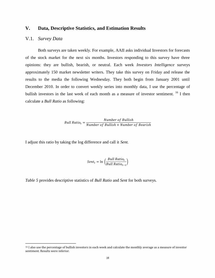
V.1. Survey Data
Both surveys are taken weekly. For example, AAII asks individual Investors for forecasts
of the stock market for the next six months. Investors responding to this survey have three
opinions: they are bullish, bearish, or neutral. Each week Investors Intelligence surveys
approximately 150 market newsletter writers. They take this survey on Friday and release the
results to the media the following Wednesday. They both begin from January 2001 until
December 2010. In order to convert weekly series into monthly data, I use the percentage of
bullish investors in the last week of each month as a measure of investor sentiment. 16
I then
calculate a Bull Ratio as following:
I adjust this ratio by taking the log difference and call it Sent.
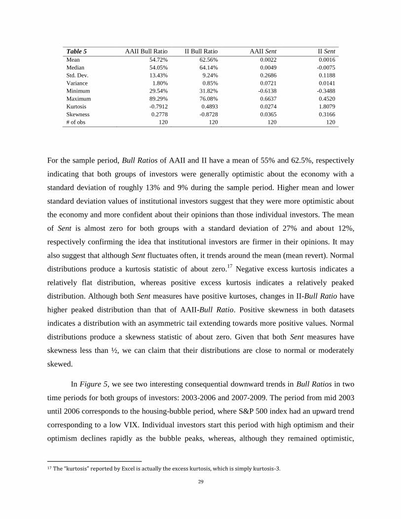
Table 5 provides descriptive statistics of Bull Ratio and Sent for both surveys.
16 I also use the percentage of bullish investors in each week and calculate the monthly average as a measure of investor sentiment. Results were inferior.
29
Table 5 AAII Bull Ratio II Bull Ratio AAII Sent II Sent
Mean 54.72% 62.56% 0.0022 0.0016
Median 54.05% 64.14% 0.0049 -0.0075
Std. Dev. 13.43% 9.24% 0.2686 0.1188
Variance 1.80% 0.85% 0.0721 0.0141
Minimum 29.54% 31.82% -0.6138 -0.3488
Maximum 89.29% 76.08% 0.6637 0.4520
Kurtosis -0.7912 0.4893 0.0274 1.8079
Skewness 0.2778 -0.8728 0.0365 0.3166
# of obs 120 120 120 120
For the sample period, Bull Ratios of AAII and II have a mean of 55% and 62.5%, respectively
indicating that both groups of investors were generally optimistic about the economy with a
standard deviation of roughly 13% and 9% during the sample period. Higher mean and lower
standard deviation values of institutional investors suggest that they were more optimistic about
the economy and more confident about their opinions than those individual investors. The mean
of Sent is almost zero for both groups with a standard deviation of 27% and about 12%,
respectively confirming the idea that institutional investors are firmer in their opinions. It may
also suggest that although Sent fluctuates often, it trends around the mean (mean revert). Normal
distributions produce a kurtosis statistic of about zero.17
Negative excess kurtosis indicates a
relatively flat distribution, whereas positive excess kurtosis indicates a relatively peaked
distribution. Although both Sent measures have positive kurtoses, changes in II-Bull Ratio have
higher peaked distribution than that of AAII-Bull Ratio. Positive skewness in both datasets
indicates a distribution with an asymmetric tail extending towards more positive values. Normal
distributions produce a skewness statistic of about zero. Given that both Sent measures have
skewness less than ½, we can claim that their distributions are close to normal or moderately
skewed.
In Figure 5, we see two interesting consequential downward trends in Bull Ratios in two
time periods for both groups of investors: 2003-2006 and 2007-2009. The period from mid 2003
until 2006 corresponds to the housing-bubble period, where S&P 500 index had an upward trend
corresponding to a low VIX. Individual investors start this period with high optimism and their
optimism declines rapidly as the bubble peaks, whereas, although they remained optimistic,
17 The “kurtosis” reported by Excel is actually the excess kurtosis, which is simply kurtosis-3.

30
institutional investors' optimism did not die out so rapidly. This is consistent with Shefrin and
Statman's (1985) "disposition effect", where individual investors are more emotional than
professional investors and likely to sell their winning stocks too early in order to postpone the
regret associated with realizing a loss. The second downward trend corresponds to the period of
2008 financial meltdown, this time where we see a rapid decline in institutional investors' Bull
Ratio, relatively speaking. Although they do not get as emotional as individual investors,
institutional investors show a great degree of pessimism during the housing crisis.
Figure 5
0%
10%
20%
30%
40%
50%
60%
70%
80%
90%
100%
AAII Bull Ratio
-0.8
-0.6
-0.4
-0.2
0.0
0.2
0.4
0.6
0.8
1.0AAII Sent
0%
10%
20%
30%
40%
50%
60%
70%
80%
Jan
-01
Nov-0
1
Sep
-02
Jul-
03
May
-04
Mar
-05
Jan
-06
Nov-0
6
Sep
-07
Jul-
08
May
-09
Mar
-10
IIBR
-0.4
-0.3
-0.2
-0.1
0
0.1
0.2
0.3
0.4
0.5
Jan
-01
Oct
-01
Jul-
02
Apr-
03
Jan
-04
Oct
-04
Jul-
05
Apr-
06
Jan
-07
Oct
-07
Jul-
08
Apr-
09
Jan
-10
Oct
-10
II Sent
31
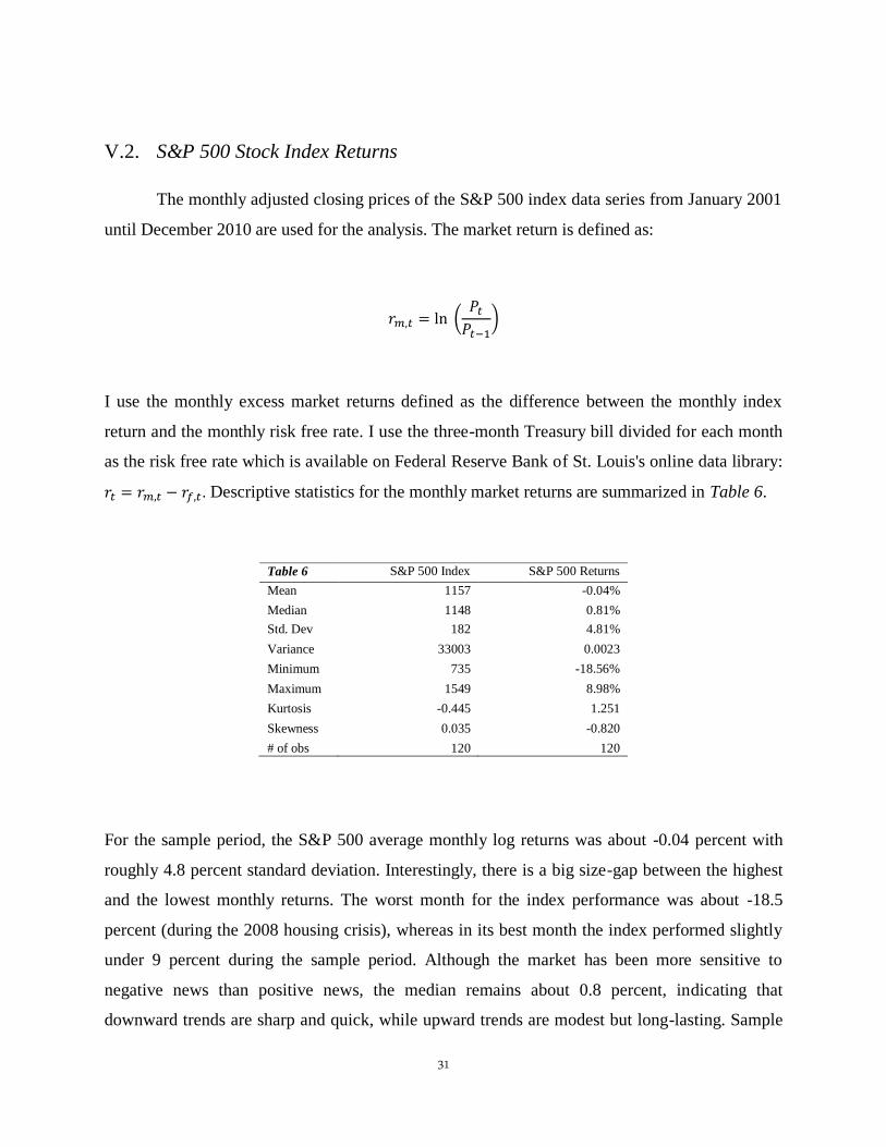
V.2. S&P 500 Stock Index Returns
The monthly adjusted closing prices of the S&P 500 index data series from January 2001
until December 2010 are used for the analysis. The market return is defined as:
I use the monthly excess market returns defined as the difference between the monthly index
return and the monthly risk free rate. I use the three-month Treasury bill divided for each month
as the risk free rate which is available on Federal Reserve Bank of St. Louis's online data library:
. Descriptive statistics for the monthly market returns are summarized in Table 6.
Table 6 S&P 500 Index S&P 500 Returns
Mean 1157 -0.04%
Median 1148 0.81%
Std. Dev 182 4.81%
Variance 33003 0.0023
Minimum 735 -18.56%
Maximum 1549 8.98%
Kurtosis -0.445 1.251
Skewness 0.035 -0.820
# of obs 120 120
For the sample period, the S&P 500 average monthly log returns was about -0.04 percent with
roughly 4.8 percent standard deviation. Interestingly, there is a big size-gap between the highest
and the lowest monthly returns. The worst month for the index performance was about -18.5
percent (during the 2008 housing crisis), whereas in its best month the index performed slightly
under 9 percent during the sample period. Although the market has been more sensitive to
negative news than positive news, the median remains about 0.8 percent, indicating that
downward trends are sharp and quick, while upward trends are modest but long-lasting. Sample

32
kurtosis is greater than one, indicating that the returns have a peaked distribution. From the
skewness, negative excess skewness is observed, leading to high Jarque-Bera statistics indicating
non-normality.
Figure 6
Figure 6 confirms those statistics in Table 6. We see two dips: One is around October
2002 following the 2000-dot-com bubble and the other one is around March 2009 following the
2008-housing crisis. During the dot-com crisis the index lost nearly 50 percent of its value in the
following subsequent 3 years and it took nearly 5 years to reach back to where it was before the
crisis. The impact of the 2008-housing crisis on the index was more severe. It lost about 56
percent of its value in slightly less than two years and it has been recovering slowly since as we
speak. We also observe that index returns were mostly positive and less volatile fluctuating
roughly plus-minus five percent during 2003-2007, consistent with the hypothesis that VIX is
low during an expansion period.
V.3. Estimations Results for Sentiment Measures
V.3.1. Individual Investor Sentiment
I use ten selected macro variables to estimate the coefficients for individual investors
survey. Table 7 reports summary statistics for the estimated coefficients.
0
200
400
600
800
1000
1200
1400
1600
1800
Jan
-01
No
v-01
Sep
-02
Jul-
03
May
-04
Mar
-05
Jan
-06
No
v-06
Sep
-07
Jul-
08
May
-09
Mar
-10
S&P 500 Index
-0.2
-0.15
-0.1
-0.05
0
0.05
0.1
0.15
Jan
-01
No
v-01
Sep
-02
Jul-
03
May
-04
Mar
-05
Jan
-06
No
v-06
Sep
-07
Jul-
08
May
-09
Mar
-10
S&P 500 Return

33
Table 7 Individual Investor Sentiment (AAII)
Estimate Std. Error t-value Pr(>|t|)
(Intercept) 0.0322 0.0289 1.114 0.2677 Disposable Income -0.0022 0.0012 -1.800 0.0746 *
Retail Sales 0.0657 0.0264 2.490 0.0143 ** PPI -0.0278 0.0123 -2.259 0.0259 **
YC 0.1999 0.0855 2.339 0.0212 ** Euro Dollar 1.6920 0.8086 2.093 0.0387 **
Job Openings in Manufacture 0.0025 0.0009 2.808 0.0059 *** Inventory to Sales 3.3100 1.8220 1.816 0.0721 *
Expenditure to Income -26.5300 12.9700 -2.045 0.0432 **
Trade Balance -0.0251 0.0077 -3.273 0.0014 ***
Housing -0.0005 0.0002 -2.224 0.0282 **
R-squared 22.05%
Adjusted R-squared 14.9%
F-statistic 3.084
Observation 119
Significant Codes: 0.01 ‘***’ 0.05 ‘**’ 0.10 ‘*’
As individual investors observe a positive outlook for the economy, we expect the Bull Ratio to
go up. The sign of economic stability and growth can ignite bullishness in the market. This
period usually corresponds to an economic expansion, where businesses hire more workers that
create more disposable income, which in return increases personal investment and spending that
help business sales go up. Variables positively associated with changes in the Bull Ratio which
are statistically significant include Retail Sales, Job Openings in Manufacturing, Yield Curve,
Euro Dollar, and Inventory to Sales. On the other hand, Disposable Income, Producer Price
Index, Trade Balance, Expenditure to Income, and Housing are statistically significant and
negatively associated with changes in the Bull Ratio. I regard a negative sign of Expenditure to
Income as a risk associated with people spending irresponsibly. When people spend more than
what they are earning, it makes investors more pessimistic. I also regard an unexpected negative
sign of Disposable Income as something to do with its colinearity with Expenditure to Income.
They both are highly correlated.
V.3.2. Institutional Investor Sentiment
I also use ten selected macro variables (not necessarily the same chosen for individual

34
investors) to estimate the coefficients for institutional investors survey. Table 8 reports summary
statistics for the estimated coefficients employed. Notice that some of the variables selected here
are different from those used to measure individual investor sentiment.
Table 8 Institutional Investor Sentiment (II)
Estimate Std. Error t-value Pr(>|t|)
(Intercept) -0.0047 0.0101 -0.4620 0.6452
Disposable Income 0.0001 0.0001 0.7850 0.4344
Retail Sales 0.0101 0.0056 1.7980 0.0749 *
Inventory to Sales -0.9183 0.7520 -1.2210 0.2246
Default Spread 0.1213 0.0713 1.7020 0.0917 *
Euro Dollar 0.7039 0.3080 2.2850 0.0242 **
Industrial Production -0.0281 0.0157 -1.7860 0.0768 *
Unemployment 0.0550 0.0612 0.8980 0.3713
Consumer Confidence 0.0056 0.0022 2.5450 0.0123 **
Housing -0.0001 0.0001 -0.6510 0.5163
SP500 Volume -0.0765 0.0175 -4.3830 0.0000 ***
R-squared 31.56%
Adjusted R-squared 25.28%
F-statistic 5.026
Observation 119
Significant Codes: 0.01 ‘***’ 0.05 ‘**’ 0.10 ‘*’
First of all, these selected variables explaining changes in institutional investors’ Bull Ratio do a
better job than those used for individual investors. Adjusted R-squared increased substantially.
Although the coefficients of Disposable Income and Inventory to Sales are insignificant, they
have the expected correct signs here. Although they both have smaller coefficients, both Retail
Sales and Euro Dollar have the same positive and significant coefficients here as well. Default
Spread has the similar positive effect but is significant here. I use four new variables measuring
institutional sentiment: Consumer Confidence Index (positive-and-significant), SP500 Volume
(negative-and-significant), Industrial Production (negative-and-significant), and Unemployment
Rate (positive-and-insignificant). The Index volume has the most significant coefficient estimate.
High volume can mean high volatility in the market place, perhaps an indication of block selloffs
and decreases in bullishness. Although we would expect a negative sign for the unemployment
rate, its coefficient is statistically insignificant. Only Industrial Production whose coefficient is
significant came out odd here. We would expect a positive sign for it.

35
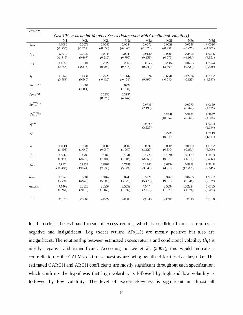
V.4. Empirical Results for Market Returns
V.4.1. GARCH-in-mean for Monthly Series (with Conditional Volatility)
I estimate the following equations using the GARCH-in-mean model with the skewed Student's
t-distribution.
(Model 1)
(Model 2.a)
(Model 2.b)
(Model 2.c)
(Model 3.a)
(Model 3.b)
(Model 3.c)
(Model 3.d)
Model 1 is the benchmark where there is no sentiment parameter. Model 2 uses investor survey
data directly, whereas in Model 3 I use fitted sentiment parameters along with their residuals.
Table 9 reports the estimation results with Robust Standard errors.
36
Table 9
GARCH-in-mean for Monthly Series (Estimation with Conditional Volatility) M1 M2a M2b M2c M3a M3b M3c M3d
-0.0059 -0.0071 -0.0040 -0.0044 -0.0071 -0.0029 -0.0056 -0.0036
(-1.593) (-1.737) (-0.938) (-0.945) (-1.620) (-0.291) (-0.229) (-0.782)
-0.1070 0.0336 0.0344 0.0643 0.0130 0.0594 -0.3488 0.0876
(-1.648) (0.407) (0.310) (0.783) (0.152) (0.678) (-4.161) (0.851)
0.0652 -0.0201 0.2622 0.2069 0.0055 0.2884 0.0753 0.2374
(0.757) (-0.213) (0.994) (0.815) (0.040) (3.769) (0.521) (1.359)
0.1142 0.1431 -0.2226 -0.1147 0.1524 -0.6340 -0.2274 -0.2952
(0.564) (0.560) (-0.429) (-0.431) (0.499) (-0.240) (-0.123) (-0.347)
0.0561 0.0227
(4.481) (1.831)
0.2630 0.2387
(8.070) (4.744)
0.0738 0.0075 0.0130
(2.490) (0.264) (0.829)
0.3149 0.2691 0.2997
(10.554) (8.067) (8.305)
0.0509 0.0253
(3.828) (2.094)
0.2437 0.2119
(9.049) (4.917)
0.0001 0.0001 0.0003 0.0002 0.0001 0.0005 0.0000 0.0002
(1.398) (1.060) (0.957) (1.067) (1.120) (0.339) (0.151) (0.790)
0.1603 0.1208 0.1166 0.1041 0.1224 0.1896 0.1137 0.1183
(1.943) (2.577) (1.481) (1.684) (2.753) (0.315) (1.915) (1.242)
0.8174 0.8636 0.6899 0.7285 0.8662 0.6624 0.8843 0.7148
(11.488) (19.544) (7.633) (5.921) (23.643) (4.215) (1233.1) (6.849)
skew 0.5749 0.6081 0.9162 0.8748 0.5921 0.9462 0.0266 0.9382
(6.591) (4.949) (5.003) (3.525) (5.476) (9.913) (0.348) (6.179)
kurtosis 9.6469 5.3310 3.2957 3.5559 4.9474 2.5094 15.2224 3.0735
(1.261) (2.010) (1.168) (1.397) (2.216) (1.328) (1.976) (1.402)
LLH 210.25 222.67 246.22 248.83 223.00 247.82 227.10 251.00
In all models, the estimated mean of excess returns, which is conditional on past returns is
negative and insignificant. Lag excess returns AR(1,2) are mostly positive but also are
insignificant. The relationship between estimated excess returns and conditional volatility ( ) is
mostly negative and insignificant. According to Lee et al. (2002), this would indicate a
contradiction to the CAPM's claim as investors are being penalized for the risk they take. The
estimated GARCH and ARCH coefficients are mostly significant throughout each specification,
which confirms the hypothesis that high volatility is followed by high and low volatility is
followed by low volatility. The level of excess skewness is significant in almost all

37
specifications. However, the models do a good job of dealing with the excess kurtosis, which is
almost insignificant in all specifications. Contrary to Fisher and Statman (2000), I found a
positive and statistically significant relationship between changes in sentiment Bull Ratio of
investors and S&P 500 excess returns in the following month (M2a, M2b). The relationship is
stronger for the institutional investors, indicating that the opinions of institutional investors
matter more relative to the opinions of individual investors on S&P 500 excess returns, which is
also confirmed when both are used together in the mean equation (M2c). Using each group of
investors separately, I found that an increase of 1.0 percentage point in the Bull Ratio of
institutional investors is associated, on average, with about 0.26 pp increase in S&P 500 excess
returns in the following month. An increase of 1.0 percentage point in the Bull Ratio of
individual investors is associated, on average, with about 0.05 pp increase in S&P 500 excess
returns in the following month. The log-likelihood values are substantially improved when
adding sentiment parameters. This suggests that these variables, when used as explanatory
variables, increase the goodness of fit in GARCH models. Test results also indicate that
observable and unobservable components of investor sentiment are important elements in
explaining S&P 500 excess returns. They are all positive and significant, suggesting that the
selected macro variables do a good job of explaining shifts in investors' Bull Ratio. For
individual investors, observable and unobservable components together have a bigger impact on
excess returns by reducing the insignificant effects of AR(1,2) on returns, compared to when it is
used directly from the surveys (M2a vs. M3a). This impact is even bigger for institutional
investors, which reduces the insignificant effect of conditional volatility ( ) on returns (M2b vs.
M3b). Again, when used together in the mean equation, the observable component of
institutional sentiment has more significant impact on excess returns than that of individual
investors (M2c vs. M3c). Lastly, the unobservable component of individual sentiment is stronger
and more significant than the observable component (M2c vs. M3c vs. M3d).
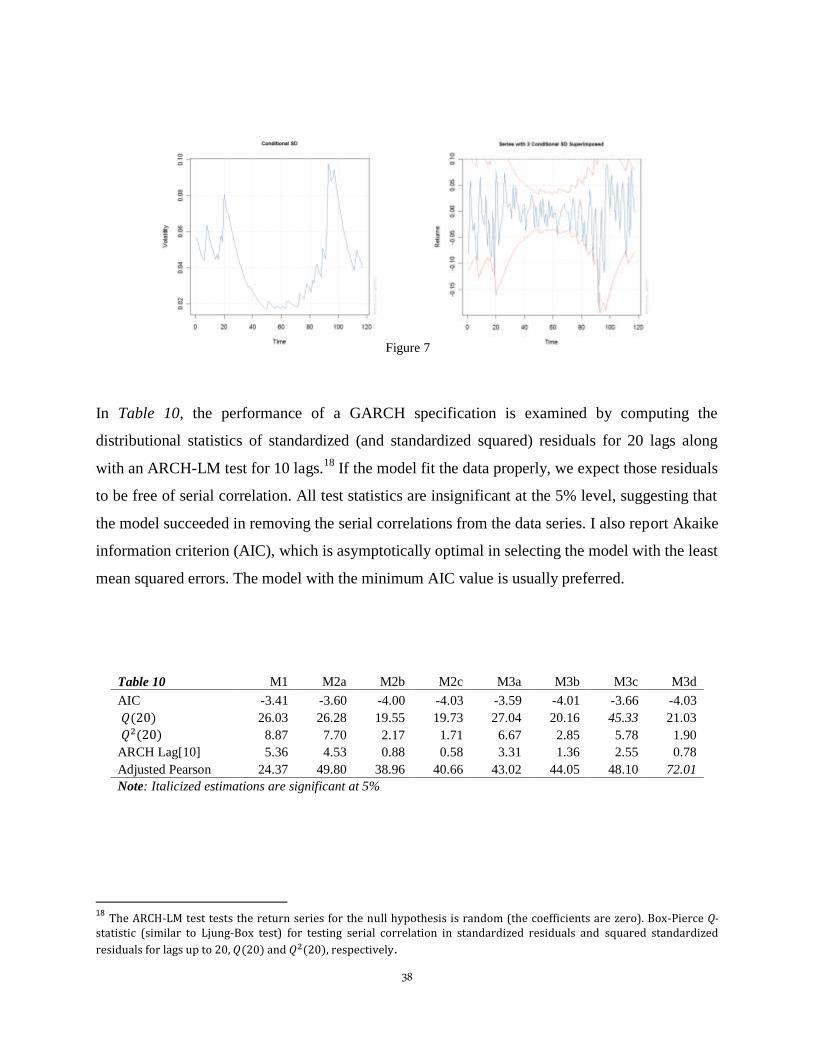
A close inspection reveals that all models capture the high volatility and subsequent
market crisis for the dot-com crisis and the housing crisis in Figure 7 below. It confirms the
hypothesis that the conditional volatility was low during the expansion period between 2003 and
2007, while it was high during both crises.
38
Figure 7
In Table 10, the performance of a GARCH specification is examined by computing the
distributional statistics of standardized (and standardized squared) residuals for 20 lags along
with an ARCH-LM test for 10 lags.18
If the model fit the data properly, we expect those residuals
to be free of serial correlation. All test statistics are insignificant at the 5% level, suggesting that
the model succeeded in removing the serial correlations from the data series. I also report Akaike
information criterion (AIC), which is asymptotically optimal in selecting the model with the least
mean squared errors. The model with the minimum AIC value is usually preferred.
Table 10 M1 M2a M2b M2c M3a M3b M3c M3d
AIC -3.41 -3.60 -4.00 -4.03 -3.59 -4.01 -3.66 -4.03
26.03 26.28 19.55 19.73 27.04 20.16 45.33 21.03
8.87 7.70 2.17 1.71 6.67 2.85 5.78 1.90
ARCH Lag[10] 5.36 4.53 0.88 0.58 3.31 1.36 2.55 0.78
Adjusted Pearson 24.37 49.80 38.96 40.66 43.02 44.05 48.10 72.01
Note: Italicized estimations are significant at 5%
18 The ARCH-LM test tests the return series for the null hypothesis is random (the coefficients are zero). Box-Pierce Q-statistic (similar to Ljung-Box test) for testing serial correlation in standardized residuals and squared standardized
residuals for lags up to 20, and , respectively.

39
V.4.2. GARCH-in-mean for Monthly Series (with Implied Volatility Data)
I repeat the analysis as in Section V.4.1 and estimate the following equations using the
GARCH(1,1) model with the skewed Student's t-distribution, where instead of adding
conditional variance in the mean equation, I add log changes in implied volatility (VIX) in the
mean equation.
(Model V.1)
(Model V.2.a)
(Model V. 2.b)
(Model V.2.c)
(Model V.3.a)
(Model V.3.b)
(Model V.3.c)
(Model V.3.d)
where
. Because index price today represents the firms' future earnings and if
implied volatility is desired to be used as a measure of risk, it should be more appropriate to add
implied volatility into the mean equation rather than past volatility.

40
Table 11
GARCH-in-mean for Monthly Series (Estimation with Implied Volatility Data) MV1 MV2a MV2b MV2c MV3a MV3b MV3c MV3d
-0.0055 -0.0052 -0.0041 -0.0040 -0.0056 -0.0039 -0.0051 -0.0037
(-1.577) (-1.579) (-1.065) (-1.018) (-1.731) (-1.008) (-0.223) (-0.924)
-0.0630 -0.0196 0.0278 0.0521 0.0006 0.0348 -0.0772 0.0666
(-0.228) (-0.216) (0.232) (0.493) (0.085) (0.273) (-0.045) (0.589)
0.1696 0.0870 0.1958 0.1827 0.0698 0.1994 0.1704 0.2000
(1.884) (0.825) (1.211) (1.382) (0.655) (1.261) (0.514) (1.705)
-0.1312 -0.1144 -0.0782 -0.0774 -0.1202 -0.0758 -0.1173 -0.0780
(-5.927) (-7.776) (-4.432) (-4.104) (-9.532) (-3.871) (-0.697) (-3.455)
0.0456 0.0206
(3.247) (2.334)
0.1872 0.1627
(6.780) (3.962)
0.0169 -0.0041 -0.0026
(0.661) (-0.072) (-0.146)
0.2088 0.1150 0.1996
(4.429) (2.118) (4.302)
0.0506 0.0260
(4.036) (2.761)
0.1840 0.1517
(7.293) (4.044)
0.0001 0.0001 0.0002 0.0001 0.0001 0.0002 0.0001 0.0001
(0.278) (1.234) (1.756) (1.383) (1.390) (1.588) (0.044) (1.371)
0.2346 0.1544 0.1763 0.1555 0.1578 0.1854 0.2030 0.1729
(0.520) (2.209) (1.587) (1.501) (2.423) (1.484) (0.129) (1.553)
0.7387 0.8076 0.6457 0.6970 0.8069 0.6379 0.7512 0.6730
(1.628) (12.556) (6.881) (6.867) (14.867) (6.508) (0.283) (5.916)
skew 0.8706 0.7467 0.8539 0.8665 0.7557 0.8669 0.8663 0.9087
(3.500) (4.516) (6.499) (7.436) (5.726) (6.505) (0.337) (8.256)
kurtosis 3.8120 4.6522 3.7873 3.6935 4.8306 3.5672 4.4480 3.8169
(0.952) (2.162) (2.040) (2.039) (2.168) (1.979) (0.217) (1.836)
LLH 235.23 245.10 258.69 261.51 246.07 258.89 238.00 262.83
Consistent with my earlier claim, Table 11 shows a negative and statistically significant
relationship between implied volatility and monthly excess returns. The estimated coefficients
have similar signs and significance, if not better, as in Table 9. The effects of both investors'
sentiment on excess returns decreased when implied volatility was added into the model, which
is more obvious for the observable component of institutional investors (M2b vs. MV2b and
M3b vs. MV3b). All models have the similar skewness as before but with more significant
kurtosis. Log-likelihood function has improved substantially throughout each specification.
41
Table 12 MV1 MV2a MV2b MV2c MV3a MV3b MV3c MV3d
AIC -3.83 -3.98 -4.22 -4.25 -3.98 -4.20 -3.85 -4.23
17.64 18.87 24.26 22.47 19.02 24.36 19.90 22.84
10.11 5.59 2.52 1.47 7.71 2.85 10.60 1.82
ARCH Lag[10] 3.46 2.58 0.78 0.41 3.93 0.92 2.75 0.55
Adjusted Pearson 40.47 44.71 34.54 61.84 41.32 44.71 45.56 66.08
Note: Italicized estimations are significant at 5%
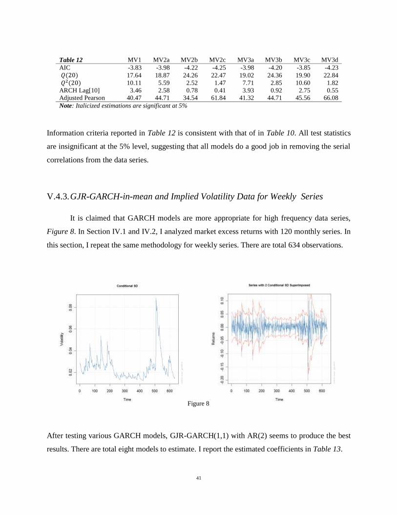
Information criteria reported in Table 12 is consistent with that of in Table 10. All test statistics
are insignificant at the 5% level, suggesting that all models do a good job in removing the serial
correlations from the data series.
V.4.3. GJR-GARCH-in-mean and Implied Volatility Data for Weekly Series
It is claimed that GARCH models are more appropriate for high frequency data series,
Figure 8. In Section IV.1 and IV.2, I analyzed market excess returns with 120 monthly series. In
this section, I repeat the same methodology for weekly series. There are total 634 observations.
Figure 8
After testing various GARCH models, GJR-GARCH(1,1) with AR(2) seems to produce the best
results. There are total eight models to estimate. I report the estimated coefficients in Table 13.

42
(Model W.1)
(Model W.2.a)
(Model W.2.b)
(Model W.2.c)
(Model W.V.3.a)
(Model W.V.3.b)
(Model W.V.3.c)
(Model W.V.3.d)
First, coefficients of conditional volatility are negative and insignificant throughout each
specification, whereas coefficients of implied volatility are negative and significant. Consistent
with monthly series, the estimated sentiment coefficients are positive and significant. Second, the
impact of changes in individual investor sentiment on weekly log returns declines when implied
volatility, rather than conditional volatility, is added into the mean equation, while the impact of
changes in institutional investor sentiment on weekly log returns remains relatively stronger in
each model. Finally, when implied volatility is used, the value of log-likelihood function is
improved substantially.

43
Table 13
GJR-GARCH-in-mean and Implied Volatility Data for Weekly Series
MW1 MW2a MW2b MW2c MWV3a MWV3b MWV3c MWV3d
0.0009 0.0011 0.0011 0.0012 0.0010 0.0010 0.0012 0.0012
(1.318) (1.849) (2.056) (2.373) (1.161) (1.180) (0.988) (1.055)
-0.1362 -0.2311 -0.2599 -0.3012 -0.0292 -0.0560 -0.1095 -0.1166
(-3.158) (-5.045) (-5.623) (-6.321) (-0.626) (-1.138) (-2.143) (-2.213)
0.0042 0.0034 -0.0583 -0.0548 0.0205 0.0330 0.0048 0.0135
(0.212) (0.259) (-1.347) (-1.242) (0.597) (0.797) (0.361) (0.362)
-0.3452 -0.4871 -0.4538 -0.5092
(-0.440) (-0.827) (-0.720) (-0.920)
-0.1235 -0.1230 -0.1182 -0.1177
(-13.518) (-13.438) (-13.969) (-13.999)
0.0220 0.0146 0.0069 0.0040
(4.669) (3.223) (2.503) (1.600)
0.1649 0.1507 0.0824 0.0795
(9.695) (8.921) (7.914) (7.631)
0.0000 0.0000 0.0000 0.0000 0.0000 0.0000 0.0000 0.0000
(7.026) (5.082) (6.291) (12.071) (0.736) (0.662) (0.286) (0.289)
0.0000 0.0000 0.0000 0.0000 0.0563 0.0495 0.0558 0.0534
(0.000) (0.000) (0.000) (0.000) (0.593) (0.511) (0.289) (0.287)
0.1319 0.1217 0.1487 0.1441 0.1553 0.1443 0.1139 0.1144
(3.755) (3.516) (3.337) (3.283) (1.816) (1.697) (0.814) (0.818)
0.9079 0.9137 0.8910 0.8950 0.8407 0.8533 0.8671 0.8695
(63.958) (74.219) (41.211) (48.807) (31.007) (34.862) (35.193) (35.013)
skew 0.7608 0.7320 0.8640 0.8450 0.9600 0.9623 1.0121 1.0149
(13.837) (11.911) (16.123) (16.111) (12.230) (12.080) (8.605) (9.205)
shape 8.9631 9.8864 7.8908 8.4624 6.3740 6.3302 5.3676 5.4142
(3.513) (3.060) (3.129) (2.877) (3.349) (3.580) (2.869) (3.020)
LLH 1503.11 1515.01 1547.35 1552.87 1756.92 1760.41 1783.94 1785.19
Table 14 confirms that all test statistics are insignificant at 5% level and all models do a good job
in removing the serial correlations from weekly series.
Table 14 MV1 MV2a MV2b MV2c MV3a MV3b MV3c MV3d
AIC -4.73 -4.76 -4.86 -4.88 -5.53 -5.54 -5.61 -5.61
13.07 16.97 20.52 21.04 25.79 26.60 28.88 29.14
20.72 20.36 9.32 9.92 15.72 15.98 11.60 11.52
ARCH Lag[10] 13.38 12.82 6.57 6.90 11.90 11.93 9.99 9.80
Adjusted Pearson 50.91 33.82 49.01 52.18 4.97 59.30 41.89 45.06
Note: Italicized estimations are significant at 5%

44
VI. Chapter Conclusion
I used various GARCH models with different combination of external variables in the
mean equation in order to build a confidence bound around the estimated coefficients. There
were fewer observations for monthly data, which is a disadvantage for GARCH models. I
include weekly series in the last section to assure that the results produced from monthly series
were consistent with a high frequency data and it can be carried on to daily series in Chapter III.
We observe that the relationship between index returns and conditional volatility ( ) remains
insignificant and inconsistent within the groups and across the GARCH models with and without
the asymmetric effect. Instead of conditional volatility, when implied volatility (VIX) is used as a
measure of risk, the goodness of fit and overall test statistics have been improved substantially.
Also adding external variables in the conditional variance such as risk free rate or using GJR-
GARCH models with AR(1) did not change the results. In this chapter, I developed a
methodology that not only measures the effects of explicit (observable) sentiment but also the
effects of implicit (unobservable) sentiment. I find a positive and statistically significant
relationship between changes in the sentiment Bull Ratio of both institutional and individual
investors and the S&P 500 excess returns in the following month. Overall, we can argue the fact
that individual investors usually follow what institutional investors do; however, test statistics
indicate that both direct and observable individual investor sentiment have less effects on S&P
500 excess returns. There might be a few reasons for this: One, they may not be following
through their opinions when they actually trade. Two, the dollar value of their investments
invested in stock market is relatively smaller than the total value invested by the institutional
investors. Three, there are other economic and market factors (which are not used here) which
can do a better job of explaining changes in observable individual investor sentiment.
Nevertheless, the selected macro variables explaining the changes in both investor sentiment
overall do a good job.

45
Chapter III
Effects of Investor Sentiment and Implied Volatility on Daily
Returns
I. Introduction
In this section, I carry out the same methodology adopted in Chapter II for daily series.
Earlier studies analyzing high frequency series use ARCH in order to capture the time series
properties (e.g., serial correlation) and to forecast underlying return volatility.19
However, those
models are often criticized because they gave little evidence on the economic forces behind the
volatility. A common approach for comparing different time series models is to ask which model
fits the data best. There is a wide acceptance of GARCH models when modeling daily stock
returns because: First, there is evidence that these models fit nonlinear return series better.
Second, the parameter estimates of GARCH models are usually statistically significant. In
Chapter I, I argue that there is a negative significant relationship between index returns and
implied volatility. In Chapter II while quantifying the effects of investor sentiment on index
returns, I show that when implied volatility is used in the mean equation, it does a better job of
explaining returns compared to conditional volatility. We can argue that there can be many
distinctly different reasons why the current value of a time series can depend nonlinearly on its
own past. However, that is not the objective here. Instead, in this chapter, combining my findings
in Chapter I and Chapter II, I investigate how current value of daily returns depends on changes
in investor sentiment and how this relationship differs under different implied (not past)
volatility states, especially when measuring daily mean reversion in returns.
19 See Diebold (1986), Stock (1987, 1988), and Lamoureux and Lastrapes (1990).

46
II. Methodology
II.1. Benchmark
In benchmark, I apply a simple GARCH methodology to determine the changes in daily
returns, which is similar to the one used in Chapter II. There are no exogenous regressors either
in the mean equation or in the variance equation. A simple model is given
by:
;
and ;
;
where : Daily S&P 500 log returns for period t:
: Mean of conditional on past information
: Variance
: Residual
II.2. Daily Returns and Measure of Investor Sentiment as a Reference Point
In behavioral finance, anchoring is a decision-making process under uncertainty, and
usually starts with a certain reference point and then adjusts it insufficiently to reach a final
conclusion. Depending on the accuracy of the reference point, the final conclusion may vary.
Fuller (1998) defines saliency as a situation in which events occur infrequently but people tend
to overestimate the probability of such an event occurring in the future if they have recently
observed such an event. He gives commercial airline crashes as an example, where if an airplane
crash is reported in the media, people will overestimate the probability of a crash occurring in the
near future. Kahneman (1992) claims that most (investment) decisions involve multiple reference
levels, which can be used to separate the time series data into the regions of desirable and
undesirable outcomes. In finance, people constantly update their beliefs as they receive financial
data. Investors put more weight on recent behaviors of stock market movements; usually the
most recent (past returns) information can be viewed as an anchor. We can observe (and
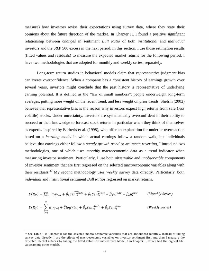
47
measure) how investors revise their expectations using survey data, where they state their
opinions about the future direction of the market. In Chapter II, I found a positive significant
relationship between changes in sentiment Bull Ratio of both institutional and individual
investors and the S&P 500 excess in the next period. In this section, I use those estimation results
(fitted values and residuals) to measure the expected market returns for the following period. I
have two methodologies that are adopted for monthly and weekly series, separately.
Long-term return studies in behavioral models claim that representative judgment bias
can create overconfidence. When a company has a consistent history of earnings growth over
several years, investors might conclude that the past history is representative of underlying
earning potential. It is defined as the ―law of small numbers‖: people underweight long-term
averages, putting more weight on the recent trend, and less weight on prior trends. Shefrin (2002)
believes that representative bias is the reason why investors expect high returns from safe (less
volatile) stocks. Under uncertainty, investors are systematically overconfident in their ability to
succeed or their knowledge to forecast stock returns in particular when they think of themselves
as experts. Inspired by Barberis et al. (1998), who offer an explanation for under or overreaction
based on a learning model in which actual earnings follow a random walk, but individuals
believe that earnings either follow a steady growth trend or are mean reverting, I introduce two
methodologies, one of which uses monthly macroeconomic data as a trend indicator when
measuring investor sentiment. Particularly, I use both observable and unobservable components
of investor sentiment that are first regressed on the selected macroeconomic variables along with
their residuals.20
My second methodology uses weekly survey data directly. Particularly, both
individual and institutional sentiment Bull Ratios regressed on market returns.
(Monthly Series)
(Weekly Series)
20 See Table 1 in Chapter II for the selected macro economic variables that are announced monthly. Instead of taking survey data directly, I use the effects of macroeconomic variables on investor sentiment first and then I measure the expected market returns by taking the fitted values estimated from Model 3 in Chapter II, which had the highest LLH value among other models.

48
where is the fitted values from the regression;
are (observable)
changes in the sentiment Bull Ratio of individual and institutional investors, which are obtained
after they are regressed on macroeconomic variables;
are the residuals
(unobservable changes in the sentiment Bull Ratio); and
are changes in the
sentiment Bull Ratio of individual and institutional investors; and is the realized S&P 500
excess returns at the end of each time period T. Recall from Section V.1 in Chapter II, in order to
convert weekly survey series into a monthly data, I use the percentage of sentiment Bull Ratio of
both investors in the last week of each month as a measure of investor sentiment. The implicit
assumption made here is that the realized market return, plays a role of an anchor when
compared to . I define gamma ( ) representing the difference between expected and
realized returns for any given time :
;
such that when gamma is positive, it is interpreted as investors being confident, bullish sentiment
and when gamma is negative, it is interpreted as investors being pessimistic, bearish sentiment.
: Bullish effect, if
: Bearish effect, if
For monthly series, Gamma ( ) measures the amount that will be reflected on the next month's
daily returns as a bullish or bearish effect. This amount will be distributed on daily returns over
the next month. However, the distribution will be weighted. Given that investors would want to
revise their expectations without any delay, the effect of revision is likely to be stronger during
the first week of the month and to die out gradually as the month continues. For any given
amount of gamma, I use the following weights, .21
For weekly series, I only use the reported
surveys directly without regressing them on selected macro economic variables. Therefore, there
is no need to convert the data into a monthly series, instead we can just use them as given in each
week. This means that we do not need to make any adjustments when distributing the effects of
21 The fifth week is added if there is more than 20-business days in a month. Also, this weighting regime is not an absolute criteria. There can be other regimes which represent the distribution better. This particular one is an illustration and is adopted for a convenience. When we use weekly series, we will not need a weighting regime.
49
investor sentiment in the dataset i.e. in each week. The following chart summarizes the
weighting regime that is used for monthly series for any given week k in a month T:
for each week k in month T
Total= 1.00
such that
for each week k
If
first week second week third week fourth week fifth week
month T-1 month T month T+1
In a contrarian strategy, some investors believe that widespread optimism (pessimism)
about market conditions can result in high (low) valuations that will eventually lead to drops
(spikes), when those expectations do not happen. The measure of gamma here is intended to
show investors' widespread optimism and pessimism. This measure is believed to have effects on
the degree of mean-reverting behavior of stock returns. Earlier studies showed that the estimated
autocorrelations of short-term returns were close to zero, which provided support for the random
walk hypothesis. In the debate about stock market efficiency, Summer (1986), Poterba and
Summer (1988), and Fama and French (1988a) have shown long-term temporary deviations of
stock price from its fundamental value resulting in mean-reverting behavior of stock prices.
Choe, Nam, and Vahid (2007) argue that the sign of the first-order return autocorrelation for the
mean reversion should depend on the lag structure of the transitory components of underlying
stock prices. In Chapter II, using the AR(2)-GARCH-in-mean process, I found that the sign of
the first-order return had mixed results associated with insignificant coefficients for monthly
series. However, when AR(2)-GJR-GARCH process with implied volatility in the mean equation
was used, the sign of the first-order return was negative and significant for weekly series. In this
chapter, using GARCH(1,1) process, I first find the sign of the AR(1) process in daily returns to
be negative and significant. I then investigate the effect of investor sentiment on daily mean

50
reversion of index returns by adding the value of gamma that is multiplied by the previous day's
return. If investors are bullish (positive gamma), I expect the sign of "bullish effect" to be
positive, which reduces the degree of mean reversion, whereas if investors are bearish (negative
gamma), I expect the sign of "bearish effect" to be negative, which increases the degree of mean
reversion on daily index returns. The economic reasoning behind this relationship is that when
investors are optimistic (pessimistic) about the market, there is less (more) expected-implied
volatility in stock prices which suggests that forthcoming reversion in prices will be small
(large). The bullish and bearish effects on day t for any given week in month T is given by:
Bullish effect
Bearish effect
and
where for weekly series.
The mean and the variance equations for monthly and weekly series are given by:
;
;
or in short:
;
where ; ; ; and with the same conditional variance,
; of for captures mean reversion in daily returns and the sign of is
expected to be negative. As claimed, I argue that the degree of mean reversion depends on the
value of gamma: On average, I expect the sign of the coefficient for bullish sentiment ( to be
bearish effect bullish effect

51
positive, which reduces the negative effect of on daily returns. On the other hand, I expect the
sign of the coefficient for bearish sentiment ( to be negative, which increases the negative
effect of on daily returns.
II.3. Daily Returns, Investor Sentiment, and Implied Volatility
II.3.1. Review (Regime Switching, RS-GARCH Models)
II.3.1.1. Conventional Stochastic RS-GARCH Models
A Regime Switching GARCH (RS-GARCH) model was introduced by Hamilton (1989),
where conditional variance of the model depends on past states. Gray (1995 and 1996) improves
RS-GARCH models by introducing a path-independent GARCH process, where each conditional
variance (of stock returns) depends only on the current regime, not on the entire past history of
the process. For a three-state process, a transition diagram is given by:
where , , and are the probabilities of staying at the same regimes: regime 1, regime 2, and
regime 3, respectively. The transition matrix with three-state Markov process is given by:
=
For a three-state Markov process , assume that follows a one-order Markov
process, which can be described by transition probabilities:
Moderate
Regime
Low Regime
High
Regime

52
;
with . Each element in a transition matrix, , is the probability that state is followed
by state . For example, represents the regime switching probability of being in regime 2 at
time t given that the market was in regime 1 at time t-1. Furthermore, the sum of the each
elements in each and every row is equal to one, . Using a GARCH(1,1) model
where each conditional variance (of stock returns) depends only on the current regime, we can
define the conditional mean and the conditional variance as
where
; with ; and . is the available
information set up to time t-1. if and
are state-dependent vectors of unknown parameters. is the unobserved
regime at time t, where for each state . If the distribution of is assumed to be
normal (although it can also be a mixture of other distributions), the model can be generalized to
allow not only the parameters but also the functional forms to vary over time. For each regime i,
with probabilities , where probability distributions over three-state for
any given time t are: , , and ,
where conditional normality in each regime, represents the
cumulative normal distribution function for :
Using the Gray (1996) path independent aggregation technique, we can write the conditional
mean and conditional variance at time t as

53
where each and are given earlier for each three-state. Finally, the log-likelihood
function of normally distributed residuals for some parameters ( ) of the model can be stated
as:
where ; ; and with
We can transform and can write the log-likelihood function above for the skewed Student-t
distribution as well.
II.3.1.2. Stochastic RS-GARCH where Implied Volatility determines Regimes
In conventional regime switching (RS) GARCH models, the conditional regime
probabilities are defined on the distribution of the variable (stock returns ) that is being

54
explained by the model. In Chapter II, I argue that the conditional variance of returns (when used
as a measure of time-varying risk) does a poor job compared to the implied volatility. In this
section, I propose a regime switching model where regimes are defined not within the model but
rather outside of the model particularly by implied volatility. According to the first-order Markov
process in conventional RS-GARCH models, all available information set ( ) up to the current
state is defined on the distribution of past returns, which is given by
. If we replace with , where
, we would let the current state be defined on the distribution of implied
volatility such that the information set up to the current state is written as martingale
. Under normality,
and its cumulative normal distribution
function in each state is given by:
Further, we can assume that mean and variance in each period are still stochastic and conditional
on the information set which depends on the current implied volatility level while keeping the
idea of the Gray (1996) path-independent aggregation technique and writing the conditional
mean and conditional variance at time t as:
which still have the same probability specifications:

55
but with a different cumulative normal distribution function, which is written over the
distribution of implied volatility in each period:
or we can assume a non-stochastic mean and variance such that
;
;
and the conditional mean and variance can be written as
where ; ; and ; and can be a
change in level of VIX or log-change of VIX.
II.3.2. Investor Sentiment and non-Stochastic RS-GARCH under Implied Volatility
In benchmark, we have no regimes, where a simple non-stochastic GARCH(1,1) mean
equation with implied volatility and investor sentiment is given by three equations, where the
second and the third equations are adjusted for monthly and weekly series:
;
;
;
56
.
DeBondt amd Thaler (1985) give psychological reasons why investors are subject to waves of
optimisim and pessimism when they communicate regularly and act as a group, a herding bias.
The efect of herding bias can be significant when the market is in a different volatility state. So I
define a three-regime distribution based on the historical implied volatility series: low, moderate,
and high. The daily dataset that I use starts on January 21, 1999 and ends on March 4, 2011. The
mean of VIX is roughly 22 for the sample period. I define a moderate regime as plus/minus 0.5
standard deviation from its mean.
VIX Regimes
Low :
Moderate :
High :
A simple non-stochastic GARCH(1,1) setting that allows changes in implied volatility is given
by three mean equation equations:
;
;
;
.
where and if . .
III. Empirical Results
III.1. Data and Descriptive Statistics
To capture the US stock market returns, I use the log-daily returns on S&P 500 index.
The dataset covers three periods: For the benchmark model, it starts from December 29, 1998 to

57
March 4, 2011. For investor sentiment models, the monthly series starts from March 2, 2001 to
December 31, 2010 and the weekly series starts from February 4, 1999 to March 4, 2011. Daily
returns for S&P 500 are obtained from CRSP. Implied volatility (VIX) starts from December 29,
1998 to March 4, 2011 and is obtained from the Chicago Board Options Exchange (CBOE).
Investor survey data is obtained from American Association Individual Investors, which is
assumed to represent individual investor sentiment and from Investors Intelligent, which is
assumed to represent institutional investor sentiment. Both surveys are taken weekly. Table 15
provides the descriptive statistics for daily log returns and daily log VIX. The unconditional
standard deviations of daily returns are in the range of 1.35% for the S&P 500 index and 6.07 %
for the CBOE's VIX. Both the skewness and kurtosis measures indicate that the return and
implied volatility distributions are not normal.
Table 15 Descriptive Statistics
Daily log-Returns Daily log-VIX
Mean 0.00002 -0.00007 Median 0.00052 -0.00449 Std. Dev. 0.0135 0.0607 Maximum 0.1096 0.4960 Minimum -0.0947 -0.3506 Skewness -0.112 0.532 Kurtosis 7.359 3.906 Count 3066 3066
III.2. Estimation Results
The estimated coefficients of the GARCH models are reported in Table 16. I estimate a
base model that excludes sentiment and implied volatility as explanatory variables in the mean
equation (M0). The plots for the benchmark model are given below. The first three plots
represent the series with two conditional distributions, 2.5% VaR limits and conditional standard
deviation, respectively. They indicate that the returns have had high volatility during the 2000-
dot-com crisis and the 2008-financial meltdown and have had low volatility during the expansion
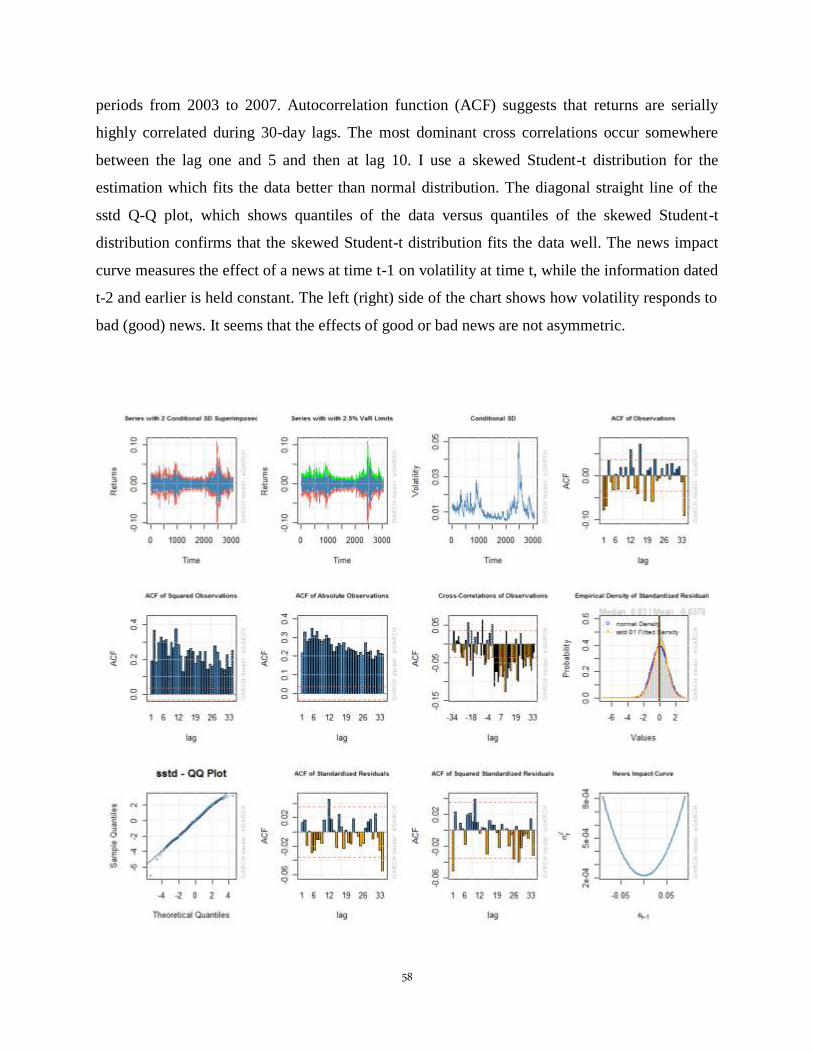
58
periods from 2003 to 2007. Autocorrelation function (ACF) suggests that returns are serially
highly correlated during 30-day lags. The most dominant cross correlations occur somewhere
between the lag one and 5 and then at lag 10. I use a skewed Student-t distribution for the
estimation which fits the data better than normal distribution. The diagonal straight line of the
sstd Q-Q plot, which shows quantiles of the data versus quantiles of the skewed Student-t
distribution confirms that the skewed Student-t distribution fits the data well. The news impact
curve measures the effect of a news at time t-1 on volatility at time t, while the information dated
t-2 and earlier is held constant. The left (right) side of the chart shows how volatility responds to
bad (good) news. It seems that the effects of good or bad news are not asymmetric.

59
Test results indicate that the mean reversion in daily returns is present and significant. A
greater degree of mean reversion in high frequency data occurs when investors are pessimistic
about the outlook of the economy, which creates high volatilities in prices. Confidence bounds
around the point estimate for the mean reversion is between -0.05 and -0.12 percentage point
(pp) for all models. Investors' bullish and bearish effects have the expected signs in mean
reversion, consistent with the earlier hypothesis. For the effect of monthly investor sentiment on
daily returns (MM0), average mean reversion is about -0.10 pp. Although bullish effect in the
mean equation is insignificant, bullish (bearish) sentiment, on average, reduces (increases) the
degree of mean reversion by 0.01 (-0.06) pp. This means that when investors are optimistic
(pessimistic), daily returns mean-revert, on average, by -0.09 pp (-0.16 pp) throughout the next
month. For the effect of weekly investor sentiment on daily returns (MW0), average mean
reversion is about -0.06 pp. Bullish (bearish) sentiment, on average, reduces (increases) the
degree of mean reversion by 0.01 (-0.04) pp throughout the next week, both of which are
significant. Adding log changes in implied volatility into the mean equation increases goodness
of fit in all specifications. A significant negative relationship between the index return and
changes in implied volatility is found in all models (M1, MM1, MW1), which is roughly -0.12
pp. The results suggest that investors are, on average, penalized for the time-varying risk they
take. When added in the mean equation, implied volatility insignificantly reduces (significantly
increases) the effect of monthly (weekly) investor sentiment, which either suggests that those
models explaining daily returns and volatility that use constantly updated (weekly) investor
sentiment do a better job when compared to the models which use monthly series or that monthly
selected macro economic variables, which are used in Chapter II, to explain the observable
component of investor sentiment need a revision. Splitting the changes in log implied volatility,
first defining them as low, moderate, and high volatility states, and then adding them as dummy
variables in the mean equation improves the test results overall. The relationship between daily
log returns and log changes in different-state implied volatility is negative and significant for all
models (M2, MM2, MW2), which are, on average, roughly -0.09 pp, -0.14 pp, and -0.22 pp,
respectively. As expected, the relationship is stronger for the high state compared to the low
state. Under these models, the effect of bullish sentiment on mean reversion has almost gone to
zero, whereas the effect of bearish sentiment has been reduced insignificantly (been increased

60
significantly) for the monthly (weekly) series. For example, for the monthly series when
investors are optimistic (pessimistic), daily returns mean-revert, on average, by -0.07 pp (-0.10
pp) throughout the next month. For the weekly series, when investors are optimistic
(pessimistic), daily returns mean-revert, on average, by -0.10 pp (-0.18 pp) throughout the next
week.
Table 16
Benchmark (without Investor Sentiment) Monthly Investor Sentiment (Indirect) Weekly Investor Sentiment (Direct)
M0 M1 M2 MM0 MM1 MM2 MW0 MW1 MW2
0.0004 0.0003 0.0005 0.0004 0.0003 0.0005 0.0004 0.0003 0.0005 (2.163) (2.756) (4.433) (1.710) (2.915) (4.154) (2.273) (2.796) (4.530)
-0.0714 -0.0621 -0.0571 -0.1019 -0.0875 -0.0723 -0.0983 -0.1152 -0.0989 (-4.703) (-3.772) (-3.229) (-2.322) (-3.878) (-3.074) (-6.263) (-5.393) (-4.369)
-0.0601 0.0076 0.0143 -0.0618 -0.0053 0.0049 -0.0630 -0.0067 0.0019 (-2.871) (1.038) (1.057) (-2.342) (-0.675) (0.254) (-3.237) (-0.509) (0.189)
-0.1255 -0.1202 -0.1254 (-23.138) (-24.377) (-23.196)
-0.0943 -0.0948 -0.0949
(-28.083) (-28.108) (-27.731)
-0.1410 -0.1371 -0.1411
(-20.276) (-17.925) (-20.518)
-0.2222 -0.2199 -0.2223
(-14.152) (-10.239) (-13.438)
Bullish Effect 0.0183 0.0123 0.0067 0.0118 0.0199 0.0000 (0.158) (0.621) (0.478) (2.483) (2.464) (1.860)
Bearish Effect -0.0696 -0.0555 -0.0379 -0.0304 -0.0506 0.0865 (-1.418) (-1.503) (-1.242) (-2.236) (-3.091) (-2.982)
0.0000 0.0000 0.0000 0.0000 0.0000 0.0000 0.0000 0.0000 0.9107 (0.211) (0.191) (0.283) (0.184) (0.122) (0.221) (0.199) (0.194) (0.262)
0.0747 0.0785 0.0823 0.0773 0.0879 0.0935 0.0747 0.0791 1.1545
(1.235) (1.141) (1.284) (1.086) (0.803) (0.971) (1.175) (1.145) (1.241)
0.9219 0.9182 0.9145 0.9185 0.9084 0.9022 0.9219 0.9175 5.6049 (15.886) (14.915) (16.750) (13.482) (9.523) (11.394) (15.114) (14.898) (15.526)
Skewness 0.8957 1.1083 1.1482 0.8899 1.1251 1.1659 0.8986 1.1124 (42.155) (38.985) (35.607) (30.676) (37.234) (30.813) (40.644) (39.211) 35.894
Kurtosis 8.9083 7.5705 5.6450 9.0766 7.4433 5.2015 8.6738 7.4946 (2.582) (3.924) (5.076) (2.074) (2.148) (3.844) (2.629) (3.534) 4.459
LLH 9550.46 10898.84 11029.41 7782.47 8884.68 8978.11 9481.25 10824.54 10947.83
# of obs 3,063 3,063 3,063 2,472 2,472 2,472 3,038 3,038 3,038
Note: t-statistics are given in parenthesis
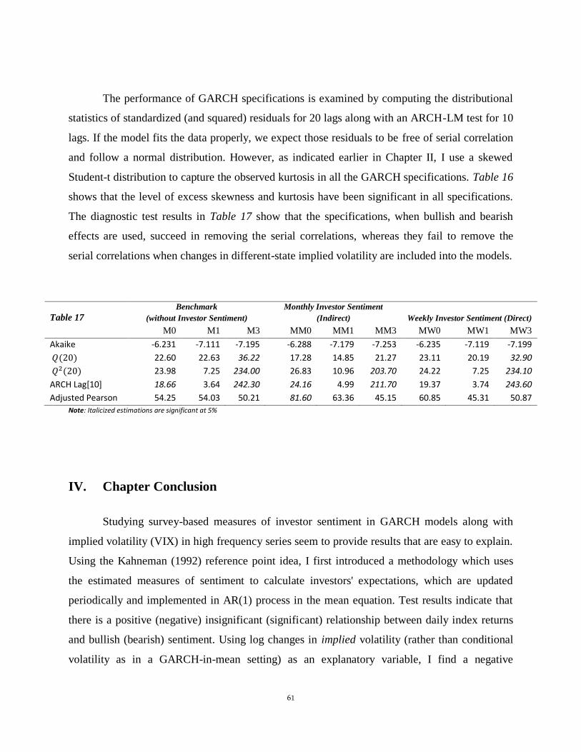
61
The performance of GARCH specifications is examined by computing the distributional
statistics of standardized (and squared) residuals for 20 lags along with an ARCH-LM test for 10
lags. If the model fits the data properly, we expect those residuals to be free of serial correlation
and follow a normal distribution. However, as indicated earlier in Chapter II, I use a skewed
Student-t distribution to capture the observed kurtosis in all the GARCH specifications. Table 16
shows that the level of excess skewness and kurtosis have been significant in all specifications.
The diagnostic test results in Table 17 show that the specifications, when bullish and bearish
effects are used, succeed in removing the serial correlations, whereas they fail to remove the
serial correlations when changes in different-state implied volatility are included into the models.
Table 17 Benchmark
(without Investor Sentiment)
Monthly Investor Sentiment
(Indirect) Weekly Investor Sentiment (Direct)
M0 M1 M3 MM0 MM1 MM3 MW0 MW1 MW3
Akaike -6.231 -7.111 -7.195 -6.288 -7.179 -7.253 -6.235 -7.119 -7.199
22.60 22.63 36.22 17.28 14.85 21.27 23.11 20.19 32.90
23.98 7.25 234.00 26.83 10.96 203.70 24.22 7.25 234.10
ARCH Lag[10] 18.66 3.64 242.30 24.16 4.99 211.70 19.37 3.74 243.60
Adjusted Pearson 54.25 54.03 50.21 81.60 63.36 45.15 60.85 45.31 50.87
Note: Italicized estimations are significant at 5%
IV. Chapter Conclusion
Studying survey-based measures of investor sentiment in GARCH models along with
implied volatility (VIX) in high frequency series seem to provide results that are easy to explain.
Using the Kahneman (1992) reference point idea, I first introduced a methodology which uses
the estimated measures of sentiment to calculate investors' expectations, which are updated
periodically and implemented in AR(1) process in the mean equation. Test results indicate that
there is a positive (negative) insignificant (significant) relationship between daily index returns
and bullish (bearish) sentiment. Using log changes in implied volatility (rather than conditional
volatility as in a GARCH-in-mean setting) as an explanatory variable, I find a negative
62
significant relationship between implied volatility and daily returns, which suggests that
investors are, on average, penalized for the time-varying risk they take. The results also suggest
that investors' pessimism (optimism) about the outlook of the economy, especially when implied
volatility is included in the mean equation, increases (decreases) the effect of mean reversion in
daily returns. This may suggest that periodic widespread pessimism causes prices to deviate from
their fundamental values, which leads the market to get into temporary correction periods. The
effects are more significant when we control the states (as low, moderate, and high volatility) of
changes in log implied volatility, especially for weekly series where investors' expectations are
calculated directly from the surveys.
V. Final Conclusion
Conventional asset pricing models mainly focus on formulating a relationship between
stock market volatility and returns and ignore the effect of investors' expectations on prices,
except those models which study noise trading where investor sentiment is viewed as irrational
or simply a noise. However, in the last couple of decades, inspired by DSSW (1990), sentiment-
based asset pricing models have gained popularity in the literature and have made significant
contributions to the field. Whaley ( 2008), Giot (2005), and Copeland and Copeland (1999) were
among others who studied the relationship between market volatility and returns and produced
significant results explaining the role of implied volatility in returns. Moreover, conventional
GARCH models introduced by Engle (1982) and Bollerslev (1986, 1987) have gained popularity
explaining volatility clustering of financial data that exhibit excess kurtosis and tail thickness.
Especially, GARCH-in-mean models which allow conditional volatility in the mean equation are
designed to measure the effects of time-varying volatility on returns. In the attempt to measure
the effect of investor sentiment on stock index returns, I use two surveys, namely changes in the
Bull Ratio of AAII (for individual investors) and II (for institutional investors) along with a set of
macroeconomic variables. I first determine what the observable component of sentiment is by
regressing the surveys' Bull Ratios on selected macroeconomic variables and I call their residuals
as unobservable component of the sentiment. Using GARCH-in-mean models, I found a positive

63
and statistically significant relationship between changes in sentiment Bull Ratio of both
investors and S&P 500 excess returns in the following month. The results indicate that the
relationship is stronger for institutional investors suggesting that the opinions of institutional
investors matter more relative to the opinions of individual investors. Instead of using
conditional volatility, I repeat the same estimation for GARCH models. The estimated
coefficients obtained from GARCH models which include exogenous implied volatility in the
mean equation have similar signs and significance with GARCH-in-mean models but the effects
of sentiment on excess returns were reduced, which is more obvious for the observable
component of institutional investors. Repeating the both methodologies for weekly series, where
I excluded selected macroeconomic variables and used surveys directly, I found consistent test
statistics. In behavioral models, it is believed that investors' widespread optimism and pessimism
can cause prices to deviate from their fundamental values, leading to temporary short or long
term corrections in the form of mean-reverting behavior when those expectations are not met.
Using periodic realized market returns as anchors, I define the difference between expected
returns, which are estimated by monthly and weekly survey-based data, and realized returns as
investor sentiment that is reflected on the daily AR(1) process, which measures the degree of
mean reversion in each period. I call it bullish (bearish) sentiment if the difference is positive
(negative). Test results indicate that there is a positive (negative) insignificant (significant)
relationship between daily index returns and bullish (bearish) sentiment, which also suggests that
investors' pessimism (optimism) about the outlook of the economy, especially when implied
volatility is controlled (as low, moderate, and high state), can increase (decrease) the effect of
mean reversion in daily returns.
References
1. ALBERG, D., SHALIT, H. and YOSEF, R 2006. "Estimating stock market volatility using asymmetric GARCH
models". Discussion Paper No. 06-10.
2. ALPERT, Marc and Howard RAIFFA 1982. ―A Progress Report on the Training of Probability Assessors,‖ in
Judgment Under Uncertainty, Cambridge University Press. Pp. 294-305.
3. BAKER, M. and Jeffrey WURGLER 2004. ―Market Liquidity as a Sentiment Indicator.‖ Journal of Financial
Markets, 7(3): 271–99.

64
4. BAKER, M. and Jeffrey WURGLER 2006. "Investor sentiment and the cross-section of stock returns. Journal of
Finance, 61(4), 1645–1680.
5. BAKER, M. and Jeffrey WURGLER 2007. "Investor Sentiment in the Stock Market". Journal of Economic
Perspectives—Volume 21, Number 2—Spring 2007—Pages 129–151.
6. BARBER, Brad M. and Terrance ODEAN 2001. ―Boys will Be Boys: Gender, Overconfidence, and Common
Stock Investment,‖ Quarterly Journal of Economics, Vol. 116(1), pp. 261-292.
7. BARBERIS, Nicholas, Andrei SHLEIFER, and Robert VISHNY 1998. "A Model of Investor Sentiment," Journal
of Financial Economics, vol. 49, no. 3 (September):307-343.
8. BARBERIS, Nicholas and Richard THALER 2003. ―A Survey of Behavioral Finance,‖ NBER Working No. 9222.
9. BLACK, Fischer 1986. ―Noise,‖ Journal of Finance, 41(3), 529–543.
10. BLACK, Fischer; SCHOLES, Myron 1973. "The Pricing of Options and Corporate Liabilities". Journal of
Political Economy81 (3): 637–654.
11. BOLLERSLEV, T., 1986. "Generalized autoregressive conditional heteroscedasticity". Journal of Econometrics
31(3), 307–327.
12. BOLLERSLEV, T., 1987. "A conditionally heteroscedastic time series model for speculative prices and rates of
13. return". Review of Economics and Statistics 69, 542–547.
14. BOLLERSLEV, T., 2008. "Glossary to ARCH (GARCH)". Oxford University Press, Oxford, UK.
15. BROWN, G.W., 1999. Volatility, sentiment, and noise traders. Financial Analysts Journal 55 (2), 82–90.
16. BROWN, G.W., and CLIFF, M. T. 2004. "Investor sentiment and the near-term stock market". Journal of
Empirical Finance, 11(1), 1–27.
17. BROWN, G.W., and CLIFF, M. T. 2005. "Investor sentiment and asset valuation". Journal of Business, 78(2),
405–440.
18. CHEN, C.R., SU, Yuli, and HUANG, Y. 2007. "Hourly index return autocorrelation and conditional volatility in an
EAR–GJR-GARCH model with generalized error distribution". Journal of Empirical Finance, 15, 789-
798.
19. CHOE, Kwang-Il & NAM, Ki Seok and VAHID, Farshid, 2007. "Necessity of negative serial correlation for mean-
reversion of stock prices". The Quarterly Review of Economics and Finance. 47, 576-583.
20. COPELAND, M. M. and COPELAND, T. E. 1999. "Market timing: Style and Size rotation using the VIX".
Financial Analysts Journal. Mar/Apr 1999; 55, 2. Page 73.
21. DANIEL, Kent, David HIRSHLEIFER, and Avanidhar SUBRAHMANYAM 1998. ―Investor Psychology and
Security Market Under- and Overreactions." Journal of Finance, vol. 53, no. 6 (December): 1839-86.
22. DE BONDT, Werner F.M. and Richard THALER 1985. ''Does the Stock Market Overreact?'' Journal of Finance,
vol. 40, no. 3 (July): 793-805.
23. DE LONG, Bradford, SHLEIFER, Andrei, SUMMERS, Lawrence, and WALDMANN, Robert J. 1990a. ―Noise
Trader Risking Financial Markets,‖ Journal of Political Economy, vol. 98, no.4.
24. DE LONG, Bradford, SHLEIFER, Andrei, SUMMERS, Lawrence, and WALDMANN, Robert J. 1990b.
―Positive Feedback Investment Strategies and Destabilizing Rational Speculation,‖ Journal of Finance 45,
375-395.
25. EDERINGTON, Louis H. and Wei GUAN Fall 2002. "Measuring Implied Volatility: Is an Average Better? Which
Average?" Journal of Futures Markets, Vol. 22 (9), 811-837.
26. ENGLE, R.F. 1982. "Autoregressive conditional heteroscedasticity with estimates of U.K. inflation". Econometrica
50. 987 1008.
27. ENGLE, R.F., LILIEN, D.M., and ROBINS, R.P., 1987. "Estimating time varying risk premia in the term
structure: The ARCH-M model". Econometrica 55, 391–407.
28. FAMA, Eugene F. and Kenneth R. FRENCH 1988. ―Permanent and Temporary Components of Stock
Prices,‖ The Journal of Political Economy, 96(2), 246–273.
29. FISCHOFF, Baruch; Paul SLOVIC, and Sarah LICHTENSTEIN 1977. "Knowing with certainty: The
appropriateness of extreme confidence". Journal of Experimental Psychology: Human Perception and
Performance 3: 552–564.
30. FISHER, K. L., and STATMAN, M. 2000. "Investor sentiment and stock returns". Financial Analysts Journal, 16–
23.

65
31. FRENCH, K.R., SCHWERT, G.W., and STAMBAUGH, R. F. 1987. "Expected stock returns and volatility".
Journal of Financial Economics 19, 3–29.
32. FULLER, Russell J. 1998. ―Behavioral Finance and the Sources of Alpha,‖ Journal of Pension Plan Investing, vol.
2, no. 3.
33. GERVAIS, S and ODEAN, T. 2001. "Learning to be Overconfident". Review of Financial Studies, Spring 2001,
Vol. 14, No. 1, pp. 1-27.
34. GIOT, P. 2005. "Implied Volatility Indexes and Daily Value at Risk Models". Journal of Derivatives. 12, 54-64.
35. GLOSTEN, L.R., JAGANNATHAN, R., and RUNKLE, D.A., 1993. "On the relation between the expected value
and the volatility of the nominal excess return on stocks". Journal of Finance 48 (5), 1779–1801.
36. GRAY, S.F., 1995. "An analysis of conditional regime-switching models", Working paper (Fuqua School of
Business, Duke University, Durham, NC).
37. GRAY, S.F. 1996. "Modeling the conditional distribution of interest rates as a regime-switching process". Journal
of Financial Economics. 42, 27-62.
38. GRIFFIN, D.W. and Amos TVERSKY 1992. ―The Weighing of Evidence and the Determinants of Confidence,‖
Cognitive Psychology, 24, 411-435.
39. GROSSMAN, Sanford J., and SHILLER, Robert J. 1981. "The Determinants of the Variability of Stock Market
Prices."The American Economic Review, Vol. 71, No. 2, (May 1981), pp. 222-227.
40. HAMILTON, J.D., 1989. "A new approach to the economic analysis of nonstationary time series and the business
cycle". Econometrica 57, 357 384.
41. HUBERMAN, Gur and Tomer REGEV 2001. ―Contagious Speculation and a Cure for Cancer: A Non-Event that
Made Stock Prices Soar In,‖ Journal of Finance,56(1), pp. 387-96.
42. KAHNEMAN, Daniel, and Amos TVERSKY 1979. "Prospect Theory: An Analysis of Decision under
Risk." Econometrica, vol. 46, no. 2 (March):171-185.
43. KAHNEMAN, Daniel, and Amos TVERSKY 1981. ―The framing of decisions and the psychology of choice,
Science 211, 453-458
44. KAHNEMAN, Daniel, and Amos TVERSKY 1982. Judgment under uncertainty: Heuristics and biases. New
York: Cambridge University Press.
45. KAHNEMAN, Daniel, and Amos TVERSKY 1992. ―Advances in prospect theory: Cumulative representation of
uncertainty‖ Journal of Risk and Uncertainty, 5(4), 297–323.
46. KAROLYI, G.A. 2001. "Why Stock Return Volatility Really Matters. Prepared for Inaugural Issue of Strategic
Investor Relations". (published by Institutional Investor Journals Series).
47. LAMBERT, P., LAURENT, S. and VEREDAS, D. 2007. "Testing conditional asymmetry: A residual-based
approach". Working Paper.
48. LAMBERT, P., and S. LAURENT 2001a. ―Modeling Financial Time Series Using GARCH Type Models and a
Skewed Student Density,‖ Discussion Paper 01-25, Institut de Statistique, Louvain-la-Neuve.
49. LAMBERT, P., and S. LAURENT 2001b. ―Modeling Skewness Dynamics in Series of Financial Data Using
Skewed Location-scale Distributions,‖ Discussion Paper 01-19, Institut de Statistique, Louvain-laNeuve.
50. LAMOUREUX, C.G. and W.D. LASTRAPES, 1990. "Persistence in variance, structural change, and the GARCH
model". Journal of Business and Economic Statistics 8, 225 234.
51. LEE, W. Y., JIANG, C. X., and INDRO, D. C. 2002. "Stock market volatility, excess returns, and the role of
investor sentiment". Journal of Banking & Finance, 26, 2277–2299.
52. LEROY, Stephen F. 1989. ―Efficient Capital Markets and Martingales,‖ Journal of Economic Literature, 27(4),
1583–1621.
53. LUCAS, Robert E., Jr., 1978. ―Asset Prices in an Exchange Economy,‖ Econometrica, 46(6), 1429–1445.
54. MALKIEL, Burton G. 2003. ―The Efficient Market Hypothesis and Its Critics,‖ Journal of Economic Perspectives,
17(1), 59–82.
55. MANDELBROT, Benoit 1963. ―The Variation of Certain Speculative Prices,‖ The Journal of Business, 36(4),
394–419.
56. MARKOWITZ, Harry M. March 1952. "Portfolio Selection," The Journal of Finance 7 (1): 77–91.
57. MARKOWITZ, Harry M. 1959. Portfolio Selection: Efficient Diversification of Investments. New York: John
Wiley & Sons. (reprinted by Yale University Press, 1970, 2nd
ed. Basil Blackwell, 1991

66
58. ODEAN, Terrance 1998. "Are Investors Reluctant to Realize Their Losses?" Journal of Finance, vol. 53, no. 5
(October):1775-98. ---1998b. "Volume, Volatility, Price and Profit When All Traders Are Above
Average." Journal of Finance, vol. 53, no. 6 (December): 1887-1934.
59. POTERBA, James M. and Lawrence H. SUMMERS 1988. ―Mean Reversion in Stock Prices: Evidence and
Implications,‖ Journal of Financial Economics, 22, 27–59.
60. SHEFRIN, Hersh and Meir STATMAN 1985. ―The Disposition to Sell Winners Too Early and Ride Losers Too
Long: Theory and Evidence,” Journal of Finance, vol XL, No 3.
61. SHLEIFER, Andrei and SUMMERS, Lawrence H. 1990. ―The Noise Trader Approach to Finance,‖ The Journal of
Economic Perspectives.
62. SHLEIFER, Andrei and Robert VISHNY 1997. "Limits of Arbitrage." Journal of Finance, vol. 52, no. 1 (March):
35-55.
63. SUMMERS, Lawrence H. 1986. ―Does the Stock Market Rationally Reflect Fundamental Values?‖ The Journal of
Finance, 41(3), 591–601.
64. VERMA, R. and SOYDEMIR, G. 2009. "The impact of individual and institutional investor sentiment on the
market price of risk". The Quarterly Review of Economics, 49, 1129-1145.
65. WHALEY, Robert E., 1993, Derivatives on market volatility: Hedging tools long overdue, Journal of Derivatives 1,
71-84.
66. WHALEY, Robert E. 2008. "Understanding VIX". Working Paper.
67. WURTZ, D. Y. CHALABI and L. LUKSA 2007. "Parameter Estimation of ARMA Models with
GARCH/APARCH Errors An R and SPlus Software Implementation". Journal of Statistical Software
(forthcoming).