Modeling radiocarbon dynamics in soils

GMDD7, 3161–3192, 2014

Radiocarbondynamics in soils

C. A. Sierra et al.

Title Page

Abstract Introduction

Conclusions References

Tables Figures

J I

J I

Back Close

Full Screen / Esc

Printer-friendly Version

Interactive Discussion

Discussion

Paper

|D

iscussionP

aper|

Discussion

Paper

|D

iscussionP

aper|

Geosci. Model Dev. Discuss., 7, 3161–3192, 2014www.geosci-model-dev-discuss.net/7/3161/2014/doi:10.5194/gmdd-7-3161-2014© Author(s) 2014. CC Attribution 3.0 License.

Open A

ccess

GeoscientificModel Development

Discussions

This discussion paper is/has been under review for the journal Geoscientific ModelDevelopment (GMD). Please refer to the corresponding final paper in GMD if available.

Modeling radiocarbon dynamics in soils:SoilR version 1.1C. A. Sierra, M. Müller, and S. E. Trumbore

Max Planck Institute for Biogeochemistry, Hans-Knöll-Str. 10, 07745 Jena, Germany

Received: 11 April 2014 – Accepted: 28 April 2014 – Published: 7 May 2014

Correspondence to: C. A. Sierra ([email protected])

Published by Copernicus Publications on behalf of the European Geosciences Union.

3161

http://www.geosci-model-dev-discuss.net

http://www.geosci-model-dev-discuss.net/7/3161/2014/gmdd-7-3161-2014-print.pdf

http://www.geosci-model-dev-discuss.net/7/3161/2014/gmdd-7-3161-2014-discussion.html

http://creativecommons.org/licenses/by/3.0/

GMDD7, 3161–3192, 2014


C. A. Sierra et al.

Title Page



Tables Figures

J I

J I

Back Close

Full Screen / Esc



Discussion

Paper

|D

iscussionP

aper|

Discussion

Paper

|D

iscussionP

aper|

Abstract

Radiocarbon is an important tracer of the global carbon cycle that helps to understandcarbon dynamics in soils. It is useful to estimate rates of organic matter cycling aswell as the mean residence or transit time of carbon in soils. We included a set offunctions to model the fate of radiocarbon in soil organic matter within the SoilR pack-5

age for the R environment for computing. Here we present the main system equationsand functions to calculate the transfer and release of radiocarbon from different soilorganic matter pools. Similarly, we present functions to calculate the mean transit timefor different pools and the entire soil system. This new version of SoilR also includesa group of datasets describing the amount of radiocarbon in the atmosphere over time,10

data necessary to estimate the incorporation of radiocarbon in soils. Also, we presentexamples on how to obtain parameters of pool-based models from radiocarbon datausing inverse parameter estimation. This implementation is general enough so it canalso be used to trace the incorporation of radiocarbon in other natural systems that canbe represented as linear dynamical systems.15

1 Introduction

To study the global carbon cycle and its interaction with climate, it is necessary todevelop models that can accurately represent the size and the amount of transfersamong different C reservoirs within the Earth system. Soils are one of the most im-portant C reservoirs, storing between 800 to 1700 PgC in the first 1 m, and exchang-20

ing between 53–57 PgCyr−1 with the atmosphere in the form of heterotrophic respira-tion (Schlesinger and Andrews, 2000; Lal, 2004; Bond-Lamberty and Thomson, 2010;Todd-Brown et al., 2013). However, there are large uncertainties in these estimations,which are related to uncertainties in C stocks of arctic peatlands, coarse woody debris,and C stocks below topsoil (Jobbágy and Jackson, 2000; Harmon et al., 2011; Todd-25

Brown et al., 2013). It is also highly debated whether climate change may destabilize

3162





GMDD7, 3161–3192, 2014


C. A. Sierra et al.

Title Page



Tables Figures

J I

J I

Back Close

Full Screen / Esc



Discussion

Paper

|D

iscussionP

aper|

Discussion

Paper

|D

iscussionP

aper|

current soil C stocks (Trumbore, 1997; Schlesinger and Andrews, 2000; Kirschbaum,2006; Davidson and Janssens, 2006; von Lützow and Kögel-Knabner, 2009; Conantet al., 2011; Sierra, 2012).

Radiocarbon can be used as a tracer of the interactions between terrestrial ecosys-tems and the atmosphere, and provides information about the rates of carbon inputs5

and losses from soils (Trumbore, 2009). Radiocarbon is a cosmogenic radionuclidethat is constantly produced in the upper layers of the stratosphere. In the lower atmo-sphere, the amount of radiocarbon at any given time is given by the balance betweencosmogenic production, radioactive decay, and sources and sinks from oceans, andthe terrestrial biosphere. Atmospheric concentrations of radiocarbon are well known10

for the past 7000–1000 years, and the continuous record even extends to 50 000 yearsinto the past (Reimer et al., 2009, 2013). Therefore, it is possible to know with goodprecision when a C atom entered the terrestrial biosphere and for how long it has beenstored in a terrestrial reservoir.

Radiocarbon is also used in tracer studies in which known amounts of radiocarbon15

label are introduced in vegetation or soils and its fate is followed as it moves amongdifferent compartments and subsequently leaves the system. During the late 1950s andearly 1960s nuclear weapon tests considerably increased the amount of radiocarbonin the atmosphere, creating a global-scale labeling experiment that allows researchersto follow the fate of this spike in atmospheric radiocarbon concentrations across many20

different reservoirs of the biosphere.In soils, radiocarbon studies have proved useful for estimating the residence times

of carbon in organic matter that cycles on time-scales ranging from years to millennia(Trumbore, 2009). Organic matter is subject to different transformation processes insoils, it can be quickly consumed by microorganisms once it enters the soil, it can be25

transformed into different compounds as a result of microbial-mediated reactions, orit can also react with soil mineral surfaces (Sollins et al., 1996; Schmidt et al., 2011;Gleixner, 2013). These different processes create a heterogeneity of rates of organicmatter decomposition that are of fundamental importance in determining long-term

3163





GMDD7, 3161–3192, 2014


C. A. Sierra et al.

Title Page



Tables Figures

J I

J I

Back Close

Full Screen / Esc



Discussion

Paper

|D

iscussionP

aper|

Discussion

Paper

|D

iscussionP

aper|

carbon stabilization in soils (Bosatta and Agren, 1991; Sierra et al., 2011). With theaid of radiocarbon measurements and models of soil organic matter decomposition, itis possible to assess this heterogeneity of decomposition rates in soils (O’Brien andStout, 1978; Bruun et al., 2004; Trumbore et al., 1996; Gaudinski et al., 2000; Baisdenand Parfitt, 2007; Brovkin et al., 2008; Trumbore, 2009).5

In this manuscript, we present the implementation of the radiocarbon componentwithin the SoilR package, a software tool developed for modeling soil organic matterdynamics (Sierra et al., 2012a). First, we present the mathematics behind the newimplementation. Then, we present some details about the numerical implementation inR and the particular functions implemented in SoilR. At the end of the manuscript, we10

present some particular examples about its use.

2 Mathematical formulation

2.1 General radiocarbon model

Previously, we have defined a general model of soil organic matter decomposition asa linear dynamical system of the form (Sierra et al., 2012a)15

dC(t)dt

= I(t)+A(t)C(t), C(t = 0) = C0 (1)

where the amount of carbon in different pools is represented as a vector C(t), withtotal inputs of carbon represented by the vector I(t). The decomposition operator A(t),a square matrix of dimension m×m, contains in its main diagonal the decomposition20

rates ki for each pool i , and coefficients representing the proportion of carbon trans-ferred from one pool to another in the off-diagonals.

3164





GMDD7, 3161–3192, 2014


C. A. Sierra et al.

Title Page



Tables Figures

J I

J I

Back Close

Full Screen / Esc



Discussion

Paper

|D

iscussionP

aper|

Discussion

Paper

|D

iscussionP

aper|

Similarly, the dynamical system for radiocarbon in soil organic matter can be repre-sented as

d14C(t)dt

= I14C(t)+A(t)14C(t)− λ14C(t), (2)

where the amount of radiocarbon in each pool i is represented by the vector 14C(t),5

with radiocarbon inputs represented by I14C(t), and λ as the radioactive decay constant.Both I14C(t) and 14C(t) represent the total amount of radiocarbon in a sample in relationto an international standard (Stuiver and Polach, 1977).

The fate of radiocarbon in soils can also be described in fractional form as

14C(t) = F (t) ◦C(t), (3)10

where F (t) is a vector of length m and ◦ represents the entry-wise product betweenthe two vectors. The fraction F (t) represents the activity ratio of a sample with respectto a reference material (see Sect. 2.2 for details, and Stuiver and Polach, 1977; Mookand Van Der Plicht, 1999). The system of equations can therefore be expressed as15

d(F (t) ◦C(t))dt

= Fa(t)I(t)+A(t) (F (t) ◦C(t))− λ (F (t) ◦C(t)), (4)

where Fa(t) is a scalar value that represents the fraction of radiocarbon in the atmo-sphere, which is not constant and has changed considerably over time due to the actionof cosmic rays, the storage and release of carbon from oceans and the biosphere, and20

human activities (Reimer et al., 2009; Levin et al., 2010; Reimer, 2012).In SoilR, we compute the time-dependent solution of Eq. (4), solving for F (t) using

standard numerical methods (see Sect. 2.4.1). F (t) contains the radiocarbon fractionfor each pool i for a given time (t).

We are also interested in calculating the total radiocarbon in soil organic matter25

weighted by its mass FC(t), and the total amount of released radiocarbon weighted

3165





GMDD7, 3161–3192, 2014


C. A. Sierra et al.

Title Page



Tables Figures

J I

J I

Back Close

Full Screen / Esc



Discussion

Paper

|D

iscussionP

aper|

Discussion

Paper

|D

iscussionP

aper|

by the total amount of released carbon FR(t). These weighted averages, or expecta-tions, can be related to the average radiocarbon content of a soil sample and the aver-age radiocarbon content of the released (respired) carbon from a sample, respectively.Mathematically, both concepts can be expressed as

FC(t) =

∑(F (t) ◦C(t))∑

C(t), (5)5

and

FR(t) =

∑(F (t) ◦R(t))∑

R(t), (6)

respectively. In both equations the sum is over all pools at each time t.10

2.2 Reporting radiocarbon

In reporting radiocarbon, there are different ways to refer to the proportion of radiocar-bon in a sample. Atmospheric radiocarbon data for the pre-bomb period is commonlyreported as ∆14C (Reimer et al., 2013), which is defined according to Stuiver and Po-lach (1977) as15

∆14C = (F −1) ·1000, (7)

with

F =ASN

AABS, (8)

20

where ASN represents the activity of a sample normalized for 13C fractionation, andAABS the activity of the oxalic acid standard normalized for 13C fractionation and cor-rected for decay since 1950.

3166





GMDD7, 3161–3192, 2014


C. A. Sierra et al.

Title Page



Tables Figures

J I

J I

Back Close

Full Screen / Esc



Discussion

Paper

|D

iscussionP

aper|

Discussion

Paper

|D

iscussionP

aper|

For post-bomb applications, radiocarbon is better expressed as F14C, which accord-ing to Reimer et al. (2004) is expressed as

F14C =ASN

AON, (9)

where AON is the activity of the oxalic acid standard with 13C normalization, but without5

decay correction; i.e.

AON = AABS ·e−λ(y−1950). (10)

Hua et al. (2013) report atmospheric radiocarbon values for the post-bomb period asF14C and as ∆14C, the later expressed as10

∆14C = (F14C ·e−λ(y−1950) −1) ·1000, (11)

i.e., the activity of the standard does not change with time during the post-bomb period.As both representations of ∆14C (Eqs. 7 and 11) are algebraically similar, we take

both types of ∆14C values and treat them equally in our calculations.15

We define an absolute fraction modern F value as

F =∆14C1000

+1, (12)

where ∆14C is expressed as Eq. (7) for radiocarbon data previous to 1950, and asEq. (11) after 1950. The system of differential equations of Eq. (4) is solved using the20

values of F as previously described.

2.3 Mean transit time

2.3.1 Definitions and assumptions

A commonly used metric to compare different compartment models is the concept ofmean transit time, also known as mean residence time (Eriksson, 1971; Bolin and25

3167





GMDD7, 3161–3192, 2014


C. A. Sierra et al.

Title Page



Tables Figures

J I

J I

Back Close

Full Screen / Esc



Discussion

Paper

|D

iscussionP

aper|

Discussion

Paper

|D

iscussionP

aper|

Rodhe, 1973; Nir and Lewis, 1975; Thompson and Randerson, 1999; Manzoni et al.,2009). In previous studies, the mean transit time of a system has been defined as theaverage time a particle of carbon spends in the system from entry to exit. This definitionhowever, has been proposed for linear time invariant (LTI) systems in which the solutiondoes not change over time and the system is in steady-state. This contrast with the5

more general models that SoilR can solve (Eqs. 1 and 2) that allow time dependentinput fluxes and decomposition rates. In addition, this definition of transit times doesnot specify the set of particles whose transit times contribute to the average, suggestingan average over all particles in the system.

Here we provide a more general definition of mean transit time that takes into account10

the more general models that SoilR can solve and specifies the set of particles usedfor calculating the average. Our formal definition states: Given a system described bythe complete history of inputs I(t) for t ∈ (tstart,t0) to all pools until time t0 and thecumulative output O(t0) of all pools at time t0 the mean transit time Tt0 of the system attime t0 is the average of the transit times of all particles leaving the system at time t0.15

Accordingly, we define the related density distribution: Given a system described bythe complete history of inputs I(t) for t ∈ (tstart,t0) to all pools until time t0 and thecumulative output O(t0) of all pools at time t0 the transit time density ψt0(T ) of thesystem at time t0 is the probability density with respect to T implicitly defined by

Tt0 =

t−tstart∫0

T ψt0(T ) dT . (13)20

Methods for calculating the mean transit time and transit time density for the generalcase and the models of the form of Eqs. (1) or (4) will be described in a forthcomingmore detailed publication. Here we will limit to describe the most common calculationof mean transit time for the LTI case, i.e. for models in steady-state (total inputs are25

equal to total outputs), constant coefficients, and constant inputs. The general form of

3168





GMDD7, 3161–3192, 2014


C. A. Sierra et al.

Title Page



Tables Figures

J I

J I

Back Close

Full Screen / Esc



Discussion

Paper

|D

iscussionP

aper|

Discussion

Paper

|D

iscussionP

aper|

these LTI models, a special case of Eq. (1), is given by

C = −A−1 · I. (14)

2.3.2 Implementation

For the LTI case, it has been shown previously that the transit time density distribution5

ψ(T ) for a transit time T is identical to the output O(T ) observed at time T of a differentsystem which started with a normalized impulsive input I

I at time T = 0 (Nir and Lewis,1975; Manzoni et al., 2009); where I represents the sum of all elements of the vectorI. Translated to the language of an ODE solver, an impulsive input becomes a vectorof initial conditions I

I at time T = 0, and Sr the release flux of the solution of the initial10

value problem observed at time T

ψ(T ) = Sr

(I

I,0,T

). (15)

Note that from the perspective of the ode solver, Sr depends only on the decomposi-tion operator A and the distribution of the input among the pools (Eq. 14). It is therefore15

possible to implement the transit time distribution as a function only of the decompo-sition operator and the fixed input flux distribution. To insure steady-state conditionsthe decomposition operator is not allowed to be a true function of time. We thereforeimplement the method only for the subclass ConstantDecompositionOperator ,a new native class of SoilR objects for the time invariant decomposition operator A.20

To compute the mean transit time for the distribution we need to compute the integral

T =

∞∫0

T ·Sr

(I

I,0,T

)dT . (16)

However, to avoid issues with numerical integration, we do not use ∞ as upper limit ofintegration, but cut the integration interval prematurely. For this purpose we calculate25

3169





GMDD7, 3161–3192, 2014


C. A. Sierra et al.

Title Page



Tables Figures

J I

J I

Back Close

Full Screen / Esc



Discussion

Paper

|D

iscussionP

aper|

Discussion

Paper

|D

iscussionP

aper|

a maximum response time of the system as (Lasaga, 1980)

τcycle =1

|min(λi )|(17)

where λi are non-zero eigenvalues of the matrix A. The upper limit of integration inEq. (16) is replaced by τcycle in or calculations.5

In future versions of SoilR, it will be possible to compute a dynamic, time-dependenttransit-time distribution for objects of class Model with a time argument specifying forwhich time the distribution is sought.

2.4 Implementation of the general radiocarbon model

The implementation of the general model of radiocarbon is similar to the implementa-10

tion of the general decomposition model presented in version 1.0 of SoilR (Sierra et al.,2012a). The system of ordinary differential equations is solved using the deSolve pack-age of Soetaert et al. (2010).

In this new version, we introduced a new set of R classes to distinguish between thetime-dependent (Eq. 1) and time-invariant (Eq. 14) versions of our general models. In15

particular, we use the virtual super class DecompOpfor different types of decomposi-tion operators, and the virtual super class InFlux for different types of input fluxes.For radiocarbon related objects, we use the classes ConstFc and BoundFc to repre-sent the radiocarbon fractions of time-invariant and time-bounded vectors, respectively.These classes must include an argument about the format of the radiocarbon values,20

either Delta14C or AbsoluteFractionModern .

2.4.1 Model initialization

All models that include radiocarbon dynamics are initialized in SoilR by the functionGeneralModel_14() . The arguments for this function are

– t : a vector containing the points in time where the solution is sought.25

3170





GMDD7, 3161–3192, 2014


C. A. Sierra et al.

Title Page



Tables Figures

J I

J I

Back Close

Full Screen / Esc



Discussion

Paper

|D

iscussionP

aper|

Discussion

Paper

|D

iscussionP

aper|

– A: a DecompOpobject consisting of a matrix valued function describing the wholemodel decay rates for the m pools, connection and feedback coefficients as func-tions of time, and a time range for which this function is valid. The dimensions ofthis matrix must be equal to the number of pools. The time range must cover thetimes given in the t argument.5

– ivList : a vector containing the initial amount of carbon for the m pools.

– initialValF an object of class ConstFc containing a vector with the initialvalues of the radiocarbon fraction for each pool and a format string describing inwhich format the values are given (Delta14C or AbsoluteFractionModern ).

– inputFluxes : an object of class InFlux consisting of a vector valued function10

describing the inputs to the pools.

– inputFc : an object of class BoundFc consisting of a function describing thefraction of 14C in per mille of the input fluxes.

– lambda : a scalar with the radiocarbon decay constant. By default, we use−0.0001209681 yr−1.15

– solverfunc : the function used to solve the ODE system. This can beSoilR.euler or deSolve.lsoda.wrapper or any other user provided func-tion with the same interface.

– pass : if set to TRUEit forces the constructor to create the model even if it violatesmass balance principles. By default, it is set ot FALSE.20

Once a model of class Model14 has been initialized, it can be queried with one ofthe functions described in Table 1. The model can also be queried by the functionsgetC , getReleaseFlux , and getAccumulatedReleaseFlux .

For models with constant coefficients, the mean transit time can be calcu-lated with the function getMeanTransitTime() applied to an object of class25

ConstLinDecompOp .3171





GMDD7, 3161–3192, 2014


C. A. Sierra et al.

Title Page



Tables Figures

J I

J I

Back Close

Full Screen / Esc



Discussion

Paper

|D

iscussionP

aper|

Discussion

Paper

|D

iscussionP

aper|

2.4.2 Radiocarbon datasets

We introduced five new datasets in SoilR to facilitate the representation and analysisof soil radiocarbon dynamics. These datasets contain information on the atmosphericradiocarbon concentration over time for different spatial and temporal domains. For thepre-bomb period, IntCal09 (Reimer et al., 2009) and IntCal13 (Reimer et al., 2013) pro-5

vide global-scale atmospheric radiocarbon data on an annual time-scale for the period0–50 000 years BP. In SoilR, these datasets are called IntCal09 and IntCal13 , re-spectively. They are implemented as data.frame with 5 variables: calibrated age inyears BP, 14C age in years BP, ∆14C value in per mil, and corresponding uncertaintyvalues for each. For additional details, see ?IntCal09 and ?IntCal13 in SoilR.10

For the post-bomb period (after 1950 AD) two additional datasets were included. Thedataset C14Atm_NHwas assembled for the Northern Hemisphere using data providedby Levin et al. (2010) and other measurements from North America. This dataset con-tains the atmospheric radiocarbon concentration in ∆14C for 111 years, form 1900 to2010 AD.15

We also included the dataset compiled by Hua et al. (2013) for four different zones inthe northern and Southern Hemispheres (Table S3 therein). This dataset, Hua2013 inSoilR, was implemented as an R list containing 5 data.frame , each representingan atmospheric zone with 5 variables. The variables are: the year AD, mean ∆14Cvalue, its standard deviation, mean F14 value, and its standard deviation.20

We also included a dataset of observations of the ∆14C value of respired CO2from soils of the Harvard Forest, MA, USA (Sierra et al., 2012b). This dataset,HarvardForest14CO2 , was implemented as a data.frame with the variables: yearof observation, ∆14C value of respired CO2, and the site of measurement within theHarvard Forest.25

3172





GMDD7, 3161–3192, 2014


C. A. Sierra et al.

Title Page



Tables Figures

J I

J I

Back Close

Full Screen / Esc



Discussion

Paper

|D

iscussionP

aper|

Discussion

Paper

|D

iscussionP

aper|

2.5 Auxiliary functions

A few functions were also introduced in this version of SoilR to help with processing ofradiocarbon data. These are:

– bind.C14curves : binds pre- and a post-bomb ∆14C curves together. The resultcan be expressed in years BP or AD.5

– AbsoluteFractionModern : transforms a ∆14C value into absolute fractionmodern using Eq. (12).

– Delta14C : transforms an absolute fraction modern value to ∆14C solvingEq. (12).

– turnoverFit : finds the turnover times of a soil sample using the ∆14C value10

measured at a particular year, the amount of litter inputs to soil, and an initialamount of C.

– PlotC14Pool : plots the output from a call to getF14 along with a radiocarboncurve.

For more details see the documentation of each function.15

3 Examples

3.1 Model structure and transit times

To interpret radiocarbon observations in soil organic matter, it is common to use mod-els with two or three pools that capture different cycling rates of carbon (O’Brien andStout, 1978; Jenkinson and Rayner, 1977; Bruun et al., 2004; Gaudinski et al., 2000;20

Trumbore, 2000). However, a multi-pool model may have different connections amongpools representing processes related to the stabilization and destabilization of organic

3173





GMDD7, 3161–3192, 2014


C. A. Sierra et al.

Title Page



Tables Figures

J I

J I

Back Close

Full Screen / Esc



Discussion

Paper

|D

iscussionP

aper|

Discussion

Paper

|D

iscussionP

aper|

matter (Sierra et al., 2011). In this example, we show how the connections among thepools may yield very different outcomes for interpreting soil radiocarbon data.

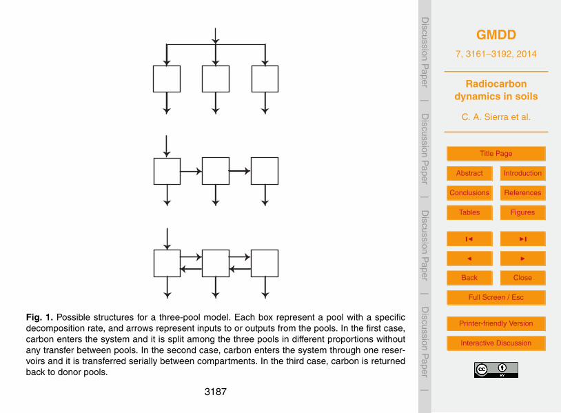
We will look at three different model structures of a three-pool model (Fig. 1), whichare special cases of the general model of Eqs. (1) and (4). In this example we willignore external environmental effects on decomposition rates, therefore we assume5

ξ(t) = 1.In the first case, carbon enters the soil and it is split among the three pools in different

proportions (γi ). Decomposition occurs in each pool independently without any transferof carbon to other compartments. We call this model three-pool parallel, and can bewritten as10

dC(t)dt

= I

γ1γ2

1−γ1 −γ2

+

−k1 0 00 −k2 00 0 −k3

C1C2C3

. (18)

In the second case, carbon enters only one of the reservoirs and it is transferred toother reservoirs in a cascade or series structure in which the residues of decompositionfrom one compartment may transfer to other compartments with lower decomposition15

rates (Swift et al., 1979; Manzoni and Porporato, 2009; Manzoni et al., 2009). Thisthree-pool series model can be expressed mathematically as

dC(t)dt

= I

100

+

−k1 0 0a21 −k2 00 a32 −k3

C1C2C3

. (19)

The third model structure considers a return of carbon residues to pools that decom-20

pose faster, mimicking processes of carbon destabilization from slowly cycling pools(Manzoni et al., 2009). Mathematically, the model can be expressed as

dC(t)dt

= I

100

+

−k1 a12 0a21 −k2 a230 a32 −k3

C1C2C3

. (20)

3174





GMDD7, 3161–3192, 2014


C. A. Sierra et al.

Title Page



Tables Figures

J I

J I

Back Close

Full Screen / Esc



Discussion

Paper

|D

iscussionP

aper|

Discussion

Paper

|D

iscussionP

aper|

To model radiocarbon dynamics under these three different assumptions of modelstructure, we transform C(t) in Eqs. (18), (19), and (20) to F (t) ◦C(t) and add a ra-diodecay term similarly as in the general models of Eqs. (1) and (4).

In SoilR, these models are implemented by the functions ThreepParallel -Model14 , ThreepSeriesModel14 , and ThreepFeedbackModel14 . We can run5

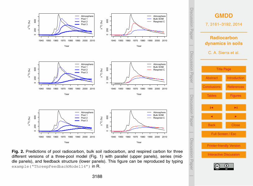
simulations for the period between the years 1901 and 2009 incorporating the at-mospheric radiocarbon record of the Northern Hemisphere in the provided datasetC14Atm_NH. Using some arbitrary initial conditions and similar decomposition ratesfor all model structures (Table 2), we can observe differences between the radiocarboncontent of the different pools as well as the radiocarbon content in the bulk soil and the10

respired CO2 (Fig. 2).Code to run these simulation is provided in the example of the func-

tion ThreepFeedbackModel14 of SoilR. To see the example simply type?ThreepFeedbackModel14 in the R command shell. To run the example typeexample(“ThreepFeedbackModel14”) .15

The simulations show that even with the same amount of inputs and decompositionrates for the three pools, the temporal behavior of radiocarbon may change significantly(Fig. 2) posing challenges for the interpretation of measured data.

Furthermore, the mean transit times of carbon obtained from these three differentmodel structures differ significantly among them. For the parallel model structure the20

mean residence time is 21 years, for the series model structure 29 years, and for thefeedback model structure 79 years. The higher the complexity of the model (number ofconnections among pools), the longer carbon stays in the system (Bruun et al., 2004;Manzoni et al., 2009), which has a direct effect on the radiocarbon signature of thedifferent pools, the bulk soil, and the respired CO2 (Fig. 2).25

3175





GMDD7, 3161–3192, 2014


C. A. Sierra et al.

Title Page



Tables Figures

J I

J I

Back Close

Full Screen / Esc



Discussion

Paper

|D

iscussionP

aper|

Discussion

Paper

|D

iscussionP

aper|

3.2 Inverse parameter estimation: fitting a one pool model to a radiocarbonsample

Soil radiocarbon data is commonly used to estimate the turnover time (τ = 1/k) ofa one-pool model. However, this is generally an ill-defined parameter estimation prob-lem because the objective is to estimate the value of one parameter from one radiocar-5

bon value. The problem gets exacerbated by the fact that there are always two possiblesolutions given the nature of the bomb-radiocarbon curve.

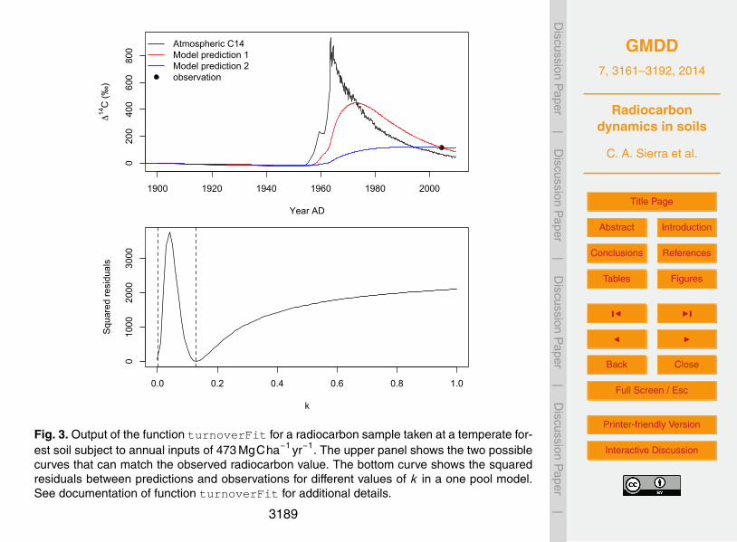
We introduced a function to estimate the two possible values of turnover time thatcan be obtained from one radiocarbon sample. This function, turnoverFit , takes asarguments the ∆14C value of the soil sample and the year of measurement, the annual10

amount of litter inputs to soil either as a constant value or as a data.frame of inputsby year. It also requires an initial amount of carbon for the first year of the simulation,and a radiocarbon hemispheric zone according to Hua et al. (2013).

The function runs an optimization algorithm that minimizes the squared differencebetween the observation and the output of OnepModel14 . It returns the two possible15

values of turnover time (τ = 1/k) that minimizes this difference between predictionsand observations and a plot that illustrates the problem (Fig. 3). An example on how torun this function for a radiocarbon sample taken at a temperate forest soil is presentedbelow.

turnoverFit(obsC14=115.22, obsyr=2004.5,20

C0=2800, yr0=1900, In=473,Zone="NHZone2")

The function runs much faster if not plot is produced, i.e. with the argumentplot=FALSE .25

One important limitation of this algorithm is the lack of uncertainty estimation for thepredicted turnover times. We do not recommend this function for formal scientific anal-yses and reporting, but rather for preliminary exploration of laboratory results. A formal

3176





GMDD7, 3161–3192, 2014


C. A. Sierra et al.

Title Page



Tables Figures

J I

J I

Back Close

Full Screen / Esc



Discussion

Paper

|D

iscussionP

aper|

Discussion

Paper

|D

iscussionP

aper|

estimation of turnover times can be achieved by performing inverse parameter estima-tion, which is described in the following example.

3.3 Inverse parameter estimation: Harvard Forest example

The assumption that soil organic carbon can be represented as a single, homoge-neous pool is generally not supported by theory and observations of soil organic mat-5

ter cycling (Swift et al., 1979; Bosatta and Agren, 1991; Trumbore, 2009; Manzoni andPorporato, 2009; Sierra et al., 2011), therefore the use of turnoverFit is not rec-ommended for heterogenous organic matter. To account for this heterogeneity, it isnecessary to use multi-pool models such as those in Fig. 2 or even more complexmodels with more pools and connections among them (e.g. O’Brien and Stout, 1978;10

Jenkinson and Rayner, 1977; Bruun et al., 2004; Gaudinski et al., 2000; Trumbore,2000; Braakhekke et al., 2014). Parameters for these models can be objectively ob-tained using inverse parameter estimation (Schädel et al., 2013; Ahrens et al., 2014;Braakhekke et al., 2014). SoilR can be coupled with R package FME (Soetaert andPetzoldt, 2010) to obtain parameter values for a specific model. We will present an15

example on how to integrate both packages and use Markov chain Monte Carlo to ob-tain parameter values for a simple model of soil organic matter dynamics derived frommeasured radiocarbon data from the Harvard Forest, USA.

Radiocarbon measurements of respired CO2 have been collected at this site for thepast decade as well as data on soil carbon stocks and proportions of organic matter20

in different fractions (Gaudinski et al., 2000; Sierra et al., 2012b). These radiocarbondata are provided in SoilR as HarvardForest14CO2 . In a previous study, we foundthat a six-pool model can reproduce very well the observed patterns of soil radiocar-bon over time (Sierra et al., 2012b). However, we are interested here in finding whethera simpler three-pool model containing roots, organic, and mineral carbon can repro-25

duce the temporal behavior observed over time. This three pool model is expressed

3177





GMDD7, 3161–3192, 2014


C. A. Sierra et al.

Title Page



Tables Figures

J I

J I

Back Close

Full Screen / Esc



Discussion

Paper

|D

iscussionP

aper|

Discussion

Paper

|D

iscussionP

aper|

as

dC(t)dt

= I

γ1γ20

+

−k1 0 0a21 −k2 0a31 0 −k3

C1C2C3

. (21)

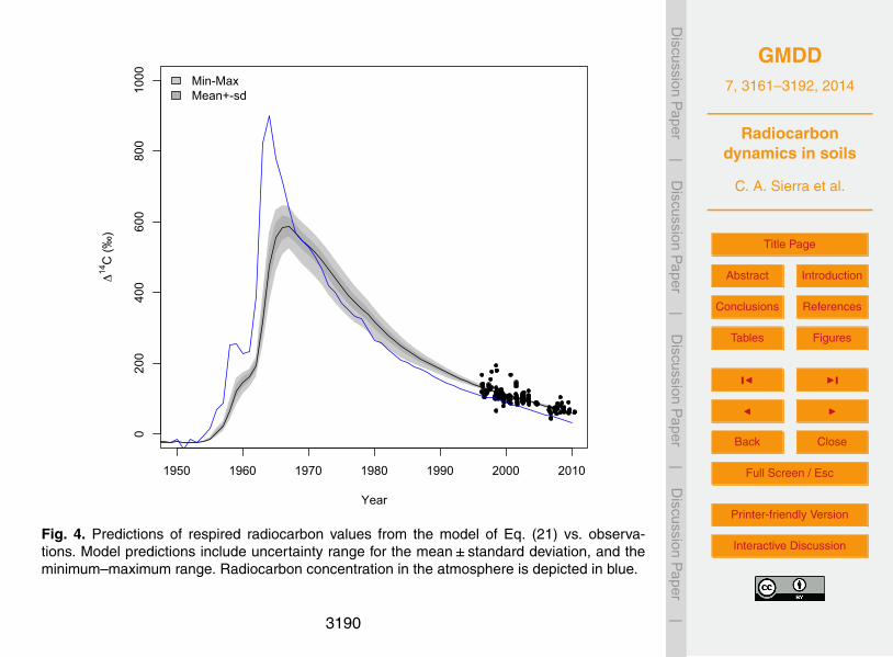
To implement this model in SoilR it is necessary to provide the arguments describedin Sect. 2.4.1 to the function GeneralModel_14 . The code for this implementation is5

presented in the supplementary material as well as the code for creating a cost functionusing package FME with the function modCost , and fitting a preliminary model to datausing the function mofFit . The mean squared residuals and the covariance matrix ofthe estimated parameters from this optimization are used to run a Markov chain MonteCarlo estimation procedure using the function modMCMC.10

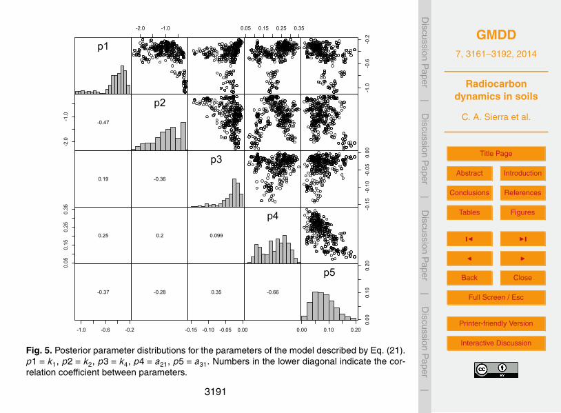
The results from this inverse parameter estimation procedure show that the modelagrees well with the observed data (Fig. 4). Similarly, the distribution of the parametersseem to indicate unimodal posterior distributions of the parameters and some degreeof correlation among them (Fig. 5).

3.4 Extrapolation of the atmospheric radiocarbon time series15

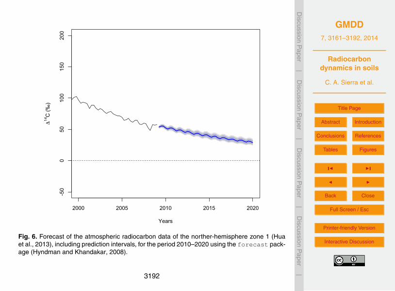
Atmospheric radiocarbon data are only released at irregular intervals to the scientificcommunity (e.g. Levin et al., 2010; Hua et al., 2013). For forward modeling of soil ra-diocarbon it is sometimes necessary to extrapolate existing data for some time into thefuture. There are a large number of tools in R for time series analyses and forecasting.For our specific problem, the forecast package (Hyndman and Khandakar, 2008)20

offers a simple and powerful extrapolation routine.The function ets in package forecast automatically finds the best possible model

for the given time series using exponential smoothing state-space modeling. Basedon the fitted model, the function forecast produces predictions forward for a givennumber of periods for forecasting.25

3178





GMDD7, 3161–3192, 2014


C. A. Sierra et al.

Title Page



Tables Figures

J I

J I

Back Close

Full Screen / Esc



Discussion

Paper

|D

iscussionP

aper|

Discussion

Paper

|D

iscussionP

aper|

Applying this procedure to the northern-hemisphere zone 1 series in Hua et al.(2013), we can forecast for example the concentration of radiocarbon in the atmo-sphere from 2010 to 2020 for this region (Fig. 6). The results from this forecast canbe subsequently merged with the original dataset and run simulations using SoilR asdescribed before. However, care must be taken with the interpretation of results using5

forecasted atmospheric radiocarbon data.

4 Conclusions

We introduced a number of functions and datasets within SoilR to model radiocarbondynamics in soil organic matter. With this tool it is possible to model the temporaldynamics of radiocarbon in soils and respired CO2 using models with any number of10

pools and connections among them. These models are generalizable to other systemswhere the incorporation of bomb radiocarbon is used to infer turnover or transit times –including human tissues, plants, sediments, etc. Radiocarbon data and other auxiliaryinformation can also be used for model identification; i.e. to obtain parameter valuesof decomposition and transfer rates in models of soil organic matter decomposition.15

This is accomplished in SoilR with an interface to R package FME, but other inverseparameter estimation methods could also be used.

Depth profiles of radiocarbon cannot be simulated with this current implementation,but this dimension will be added in a future version of SoilR.

Code availability20

SoilR version 1.1 can be obtained from the Comprehensive R Archive Network (CRAN)or RForge. Source code and test framework can be obtained from these two reposi-tories. To install, use the function install.packages(“SoilR”,repo) , specifyingeither a CRAN mirror or RForge in the repo argument.

3179





GMDD7, 3161–3192, 2014


C. A. Sierra et al.

Title Page



Tables Figures

J I

J I

Back Close

Full Screen / Esc



Discussion

Paper

|D

iscussionP

aper|

Discussion

Paper

|D

iscussionP

aper|

Supplementary material related to this article is available online athttp://www.geosci-model-dev-discuss.net/7/3161/2014/gmdd-7-3161-2014-supplement.zip.

Acknowledgements. Financial support for the development of this project has been providedby the Max Planck Society.5

The service charges for this open access publicationhave been covered by the Max Planck Society.

References

Ahrens, B., Reichstein, M., Borken, W., Muhr, J., Trumbore, S. E., and Wutzler, T.: Bayesian10

calibration of a soil organic carbon model using ∆14C measurements of soil organic car-bon and heterotrophic respiration as joint constraints, Biogeosciences, 11, 2147–2168,doi:10.5194/bg-11-2147-2014, 2014. 3177

Baisden, W. and Parfitt, R.: Bomb 14C enrichment indicates decadal C pool in deep soil?,Biogeochemistry, 85, 59–68, 2007. 316415

Bolin, B. and Rodhe, H.: A note on the concepts of age distribution and transit time in naturalreservoirs, Tellus, 25, 58–62, 1973. 3167

Bond-Lamberty, B. and Thomson, A.: Temperature-associated increases in the global soil res-piration record, Nature, 464, 579–582, doi:10.1038/nature08930, 2010. 3162

Bosatta, E. and Agren, G. I.: Dynamics of carbon and nitrogen in the organic matter of the soil:20

a generic theory, Am. Nat., 138, 227–245, 1991. 3164, 3177Braakhekke, M. C., Beer, C., Schrumpf, M., Ekici, A., Ahrens, B., Hoosbeek, M. R., Kruijt, B.,

Kabat, P., and Reichstein, M.: The use of radiocarbon to constrain current and future soilorganic matter turnover and transport in a temperate forest, J. Geophys. Res.-Biogeo., 119,372–391, doi:10.1002/2013JG002420, 2014. 317725

Brovkin, V., Cherkinsky, A., and Goryachkin, S.: Estimating soil carbon turnover us-ing radiocarbon data: a case-study for European Russia, Ecol. Model., 216, 178–187,doi:10.1016/j.ecolmodel.2008.03.018, 2008. 3164

3180





http://www.geosci-model-dev-discuss.net/7/3161/2014/gmdd-7-3161-2014-supplement.zip



http://dx.doi.org/10.5194/bg-11-2147-2014

http://dx.doi.org/10.1038/nature08930

http://dx.doi.org/10.1002/2013JG002420

http://dx.doi.org/10.1016/j.ecolmodel.2008.03.018

GMDD7, 3161–3192, 2014


C. A. Sierra et al.

Title Page



Tables Figures

J I

J I

Back Close

Full Screen / Esc



Discussion

Paper

|D

iscussionP

aper|

Discussion

Paper

|D

iscussionP

aper|

Bruun, S., Six, J., and Jensen, L. S.: Estimating vital statistics and age distributions of mea-surable soil organic carbon fractions based on their pathway of formation and radiocarboncontent, J. Theor. Biol., 230, 241–250, 2004. 3164, 3173, 3175, 3177

Conant, R. T., Ryan, M. G., Ågren, G. I., Birge, H. E., Davidson, E. A., Eliasson, P. E.,Evans, S. E., Frey, S. D., Giardina, C. P., Hopkins, F. M., Hyvönen, R., Kirschbaum, M. U. F.,5

Lavallee, J. M., Leifeld, J., Parton, W. J., Megan Steinweg, J., Wallenstein, M. D., Martin Wet-terstedt, J. Å., and Bradford, M. A.: Temperature and soil organic matter decomposition rates– synthesis of current knowledge and a way forward, Glob. Change Biol., 17, 3392–3404,2011. 3163

Davidson, E. A. and Janssens, I. A.: Temperature sensitivity of soil carbon decomposition and10

feedbacks to climate change, Nature, 440, 165–173, 2006. 3163Eriksson, E.: Compartment models and reservoir theory, Annu. Rev. Ecol. Syst., 2, 67–84,

1971. 3167Gaudinski, J., Trumbore, S., Davidson, E., and Zheng, S.: Soil carbon cycling in a temperate

forest: radiocarbon-based estimates of residence times, sequestration rates and partitioning15

fluxes, Biogeochemistry, 51, 33–69, 2000. 3164, 3173, 3177Gleixner, G.: Soil organic matter dynamics: a biological perspective derived from the use

of compound-specific isotopes studies, Ecol. Res., 28, 683–695, doi:10.1007/s11284-012-1022-9, 2013. 3163

Harmon, M. E., Bond-Lamberty, B., Tang, J., and Vargas, R.: Heterotrophic respiration in dis-20

turbed forests: lA review with examples from North America, J. Geophys. Res., 116, G00K04,doi:10.1029/2010JG001495, 2011. 3162

Hua, Q., Barbetti, M., and Rakowski, A.: Atmospheric radiocarbon for the period 1950–2010,Radiocarbon, 55, 2059–2072, 2013. 3167, 3172, 3176, 3178, 3179, 3192

Hyndman, R. J. and Khandakar, Y.: Automatic time series forecasting: the forecast package for25

R, J. Stat. Softw., 27, 1–22, 2008. 3178, 3192Jenkinson, D. S. and Rayner, J. H.: The turnover of soil organic matter in some of the rotham-

sted classical experiments, Soil Sci., 123, 298–305, 1977. 3173, 3177Jobbágy, E. and Jackson, R.: The vertical distribution of soil organic carbon and its relation to

climate and vegetation, Ecol. Appl., 10, 423–436, 2000. 316230

Kirschbaum, M. U. F.: The temperature dependence of organic-matter decomposition – still atopic of debate, Soil Biol. Biochem., 38, 2510–2518, 2006. 3163

3181





http://dx.doi.org/10.1007/s11284-012-1022-9

http://dx.doi.org/10.1007/s11284-012-1022-9

http://dx.doi.org/10.1007/s11284-012-1022-9

http://dx.doi.org/10.1029/2010JG001495

GMDD7, 3161–3192, 2014


C. A. Sierra et al.

Title Page



Tables Figures

J I

J I

Back Close

Full Screen / Esc



Discussion

Paper

|D

iscussionP

aper|

Discussion

Paper

|D

iscussionP

aper|

Lal, R.: Soil carbon sequestration impacts on global climate change and food security, Science,304, 1623–1627, 2004. 3162

Lasaga, A.: The kinetic treatment of geochemical cycles, Geochim. Cosmochim. Ac., 44, 815–828, doi:10.1016/0016-7037(80)90263-X, 1980. 3170

Levin, I., Naegler, T., Kromer, B., Diehl, M., Francey, R. J., Gomez-Pelaez, A. J., Steele, L. P.,5

Wagenbach, D., Weller, R., and Worthy, D. E.: Observations and modelling of the globaldistribution and long-term trend of atmospheric 14CO2, Tellus B, 62, 26–46, 2010. 3165,3172, 3178

Manzoni, S. and Porporato, A.: Soil carbon and nitrogen mineralization: theory and modelsacross scales, Soil Biol. Biochem., 41, 1355–1379, doi:10.1016/j.soilbio.2009.02.031, 2009.10

3174, 3177Manzoni, S., Katul, G. G., and Porporato, A.: Analysis of soil carbon transit times

and age distributions using network theories, J. Geophys. Res., 114, G04025,doi:10.1029/2009JG001070, 2009. 3168, 3169, 3174, 3175

Mook, W. and Van Der Plicht, J.: Reporting 14C activities and concentrations, Radiocarbon, 41,15

227–239, 1999. 3165Nir, A. and Lewis, S.: On tracer theory in geophysical systems in the steady and non-steady

state. Part I, Tellus, 27, 372–383, 1975. 3168, 3169O’Brien, B. J. and Stout, J. D.: Movement and turnover of soil organic matter as indicated

by carbon isotope measurements, Soil Biol. Biochem., 10, 309–317, doi:10.1016/0038-20

0717(78)90028-7, 1978. 3164, 3173, 3177Reimer, P., Brown, T., and Reimer, R.: Reporting and Calibration of Post-Bomb 14C Data,

Radiocarbon, 46, 1299–1304, 2004. 3167Reimer, P. J., Baillie, M. G. L., Bard, E., Bayliss, A., Beck, J. W., Blackwell, P. J., Bronk Ramsey,

C., Buck, C. E., Burr, G. S., Edwards, R. L., Friedrich, M., Grootes, P. M., Guilderson, T. P.,25

Hajdas, I., Heaton, T. J., Hogg, A. G., Hughen, K. A., Kaiser, K. F., Kromer, B., McCormac,F. G., Manning, S. W., Reimer, R. W., Richards, D. A., Southon, J. R., Talamo, S., Turney, C.S. M., van der Plicht, J., and Weyhenmeyer C. E.: IntCal09 and Marine09 radiocarbon agecalibration curves, 0–50,000 years cal BP, Radiocarbon, 51, 1111–1150, 2009. 3163, 3165,317230

Reimer, P., Bard, E., Bayliss, A., Beck, J., Blackwell, P., Ramsey, C. B., Grootes, P., Guilder-son, T., Haflidason, H., Hajdas, I., Hatté, C., Heaton, T., Hoffmann, D., Hogg, A., Hughen, K.,Kaiser, K., Kromer, B., Manning, S., Niu, M., Reimer, R., Richards, D., Scott, E., Southon, J.,

3182





http://dx.doi.org/10.1016/0016-7037(80)90263-X

http://dx.doi.org/10.1016/j.soilbio.2009.02.031

http://dx.doi.org/10.1029/2009JG001070

http://dx.doi.org/10.1016/0038-0717(78)90028-7

http://dx.doi.org/10.1016/0038-0717(78)90028-7

http://dx.doi.org/10.1016/0038-0717(78)90028-7

GMDD7, 3161–3192, 2014


C. A. Sierra et al.

Title Page



Tables Figures

J I

J I

Back Close

Full Screen / Esc



Discussion

Paper

|D

iscussionP

aper|

Discussion

Paper

|D

iscussionP

aper|

Staff, R., Turney, C., and van der Plicht, J.: IntCal13 and Marine13 radiocarbon age calibra-tion curves 0–50,000 years cal BP, Radiocarbon, 55, 1869–1887, 2013. 3163, 3166, 3172

Reimer, P. J.: Refining the radiocarbon time scale, Science, 338, 337–338,doi:10.1126/science.1228653, 2012. 3165

Schädel, C., Luo, Y., David Evans, R., Fei, S., and Schaeffer, S.: Separating soil CO2 efflux5

into C-pool-specific decay rates via inverse analysis of soil incubation data, Oecologia, 171,721–732, doi:10.1007/s00442-012-2577-4, 2013. 3177

Schlesinger, W. H. and Andrews, J. A.: Soil respiration and the global carbon cycle, Biogeo-chemistry, 48, 7–20, 2000. 3162, 3163

Schmidt, M. W. I., Torn, M. S., Abiven, S., Dittmar, T., Guggenberger, G., Janssens, I. A., Kle-10

ber, M., Kogel-Knabner, I., Lehmann, J., Manning, D. A. C., Nannipieri, P., Rasse, D. P.,Weiner, S., and Trumbore, S. E.: Persistence of soil organic matter as an ecosystem prop-erty, Nature, 478, 49–56, 2011. 3163

Sierra, C.: Temperature sensitivity of organic matter decomposition in the Arrhenius equation:some theoretical considerations, Biogeochemistry, 108, 1–15, 2012. 316315

Sierra, C. A., Harmon, M. E., and Perakis, S. S.: Decomposition of heterogeneous organicmatter and its long-term stabilization in soils, Ecol. Monogr., 81, 619–634, doi:10.1890/11-0811.1, 2011. 3164, 3174, 3177

Sierra, C. A., Müller, M., and Trumbore, S. E.: Models of soil organic matter decomposition: theSoilR package, version 1.0, Geosci. Model Dev., 5, 1045–1060, doi:10.5194/gmd-5-1045-20

2012, 2012a. 3164, 3170Sierra, C. A., Trumbore, S. E., Davidson, E. A., Frey, S. D., Savage, K. E., and Hopkins, F. M.:

Predicting decadal trends and transient responses of radiocarbon storage and fluxes in atemperate forest soil, Biogeosciences, 9, 3013–3028, doi:10.5194/bg-9-3013-2012, 2012b.3172, 317725

Soetaert, K. and Petzoldt, T.: Inverse modelling, sensitivity and Monte Carlo analysis in R usingpackage FME, J. Stat. Softw., 33, 1–28, 2010. 3177

Soetaert, K., Petzoldt, T., and Setzer, R.: Solving differential equations in R: Package deSolve,J. Stat. Softw., 33, 1–25, 2010. 3170

Sollins, P., Homann, P., and Caldwell, B. A.: Stabilization and destabilization of soil organic mat-30

ter: mechanisms and controls, Geoderma, 74, 65–105, doi:10.1016/S0016-7061(96)00036-5, 1996. 3163

3183





http://dx.doi.org/10.1126/science.1228653

http://dx.doi.org/10.1007/s00442-012-2577-4

http://dx.doi.org/10.1890/11-0811.1

http://dx.doi.org/10.1890/11-0811.1

http://dx.doi.org/10.1890/11-0811.1

http://dx.doi.org/10.5194/gmd-5-1045-2012



http://dx.doi.org/10.5194/bg-9-3013-2012

http://dx.doi.org/10.1016/S0016-7061(96)00036-5

http://dx.doi.org/10.1016/S0016-7061(96)00036-5

http://dx.doi.org/10.1016/S0016-7061(96)00036-5

GMDD7, 3161–3192, 2014


C. A. Sierra et al.

Title Page



Tables Figures

J I

J I

Back Close

Full Screen / Esc



Discussion

Paper

|D

iscussionP

aper|

Discussion

Paper

|D

iscussionP

aper|

Stuiver, M. and Polach, H. A.: Reporting of C-14 data, Radiocarbon, 19, 355–363, 1977. 3165,3166

Swift, M. J., Heal, O. W., and Anderson, J. M.: Decomposition in Terrestrial Ecosystems, Uni-versity of California Press, Berkeley, 1979. 3174, 3177

Thompson, M. V. and Randerson, J. T.: Impulse response functions of terrestrial carbon cy-5

cle models: method and application, Glob. Change Biol., 5, 371–394, doi:10.1046/j.1365-2486.1999.00235.x, 1999. 3168

Todd-Brown, K. E. O., Randerson, J. T., Post, W. M., Hoffman, F. M., Tarnocai, C.,Schuur, E. A. G., and Allison, S. D.: Causes of variation in soil carbon simulations fromCMIP5 Earth system models and comparison with observations, Biogeosciences, 10, 1717–10

1736, doi:10.5194/bg-10-1717-2013, 2013. 3162Trumbore, S.: Age of soil organic matter and soil respiration: radiocarbon constraints on below-

ground C dynamics, Ecol. Appl., 10, 399–411, 2000. 3173, 3177Trumbore, S.: Radiocarbon and soil carbon dynamics, Annu. Rev. Earth Pl. Sc., 37, 47–66,

2009. 3163, 3164, 317715

Trumbore, S. E.: Potential responses of soil organic carbon to global environmental change, P.Natl. Acad. Sci. USA, 94, 8284–8291, 1997. 3163

Trumbore, S. E., Chadwick, O. A., and Amundson, R.: Rapid exchange between soil carbon andatmospheric carbon dioxide driven by temperature change, Science, 272, 393–396, 1996.316420

von Lützow, M. and Kögel-Knabner, I.: Temperature sensitivity of soil organic matter decompo-sition – what do we know?, Biol. Fert. Soils, 46, 1–15, 2009. 3163

3184





http://dx.doi.org/10.1046/j.1365-2486.1999.00235.x

http://dx.doi.org/10.1046/j.1365-2486.1999.00235.x

http://dx.doi.org/10.1046/j.1365-2486.1999.00235.x

http://dx.doi.org/10.5194/bg-10-1717-2013

GMDD7, 3161–3192, 2014


C. A. Sierra et al.

Title Page



Tables Figures

J I

J I

Back Close

Full Screen / Esc



Discussion

Paper

|D

iscussionP

aper|

Discussion

Paper

|D

iscussionP

aper|

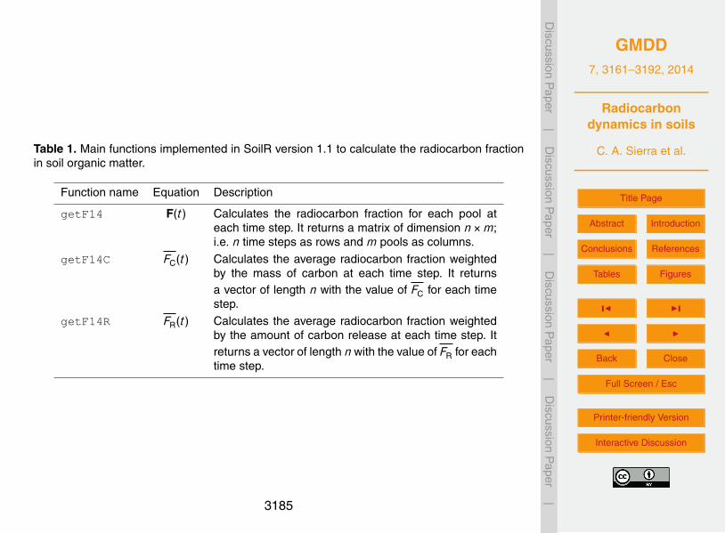
Table 1. Main functions implemented in SoilR version 1.1 to calculate the radiocarbon fractionin soil organic matter.

Function name Equation Description

getF14 F(t) Calculates the radiocarbon fraction for each pool ateach time step. It returns a matrix of dimension n×m;i.e. n time steps as rows and m pools as columns.

getF14C FC(t) Calculates the average radiocarbon fraction weightedby the mass of carbon at each time step. It returnsa vector of length n with the value of FC for each timestep.

getF14R FR(t) Calculates the average radiocarbon fraction weightedby the amount of carbon release at each time step. Itreturns a vector of length n with the value of FR for eachtime step.

3185





GMDD7, 3161–3192, 2014


C. A. Sierra et al.

Title Page



Tables Figures

J I

J I

Back Close

Full Screen / Esc



Discussion

Paper

|D

iscussionP

aper|

Discussion

Paper

|D

iscussionP

aper|

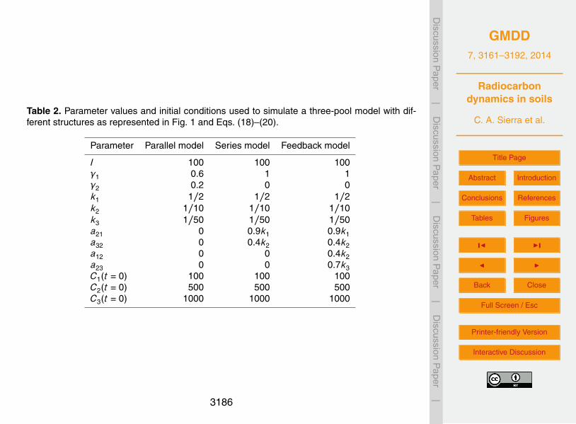
Table 2. Parameter values and initial conditions used to simulate a three-pool model with dif-ferent structures as represented in Fig. 1 and Eqs. (18)–(20).

Parameter Parallel model Series model Feedback model

I 100 100 100γ1 0.6 1 1γ2 0.2 0 0k1 1/2 1/2 1/2k2 1/10 1/10 1/10k3 1/50 1/50 1/50a21 0 0.9k1 0.9k1a32 0 0.4k2 0.4k2a12 0 0 0.4k2a23 0 0 0.7k3C1(t = 0) 100 100 100C2(t = 0) 500 500 500C3(t = 0) 1000 1000 1000

3186





GMDD7, 3161–3192, 2014


C. A. Sierra et al.

Title Page



Tables Figures

J I

J I

Back Close

Full Screen / Esc



Discussion

Paper

|D

iscussionP

aper|

Discussion

Paper

|D

iscussionP

aper|

6 Sierra et al.: Radiocarbon dynamics in soils

Fig. 1. Possible structures for a three-pool model. Each box repre-sent a pool with a specific decomposition rate, and arrows representinputs to or outputs from the pools. In the first case, carbon entersthe system and it is split among the three pools in different propor-tions without any transfer between pools. In the second case, carbonenters the system through one reservoirs and it is transferred seriallybetween compartments. In the third case, carbon is returned back todonor pools.

of carbon destabilization from slowly cycling pools (Man-415

zoni et al., 2009). Mathematically, the model can be ex-pressed as

dC(t)

dt= I

100

+

−k1 a12 0a21 −k2 a23

0 a32 −k3

C1

C2

C3

. (20)

To model radiocarbon dynamics under these three differ-ent assumptions of model structure, we transform C(t) in420

equations 18, 19, and 20 to F (t)◦C(t) and add a radiodecayterm similarly as in the general models of equations 1 and 4.

In SoilR, these models are implemented bythe functions ThreepParallelModel14,ThreepSeriesModel14, and425

ThreepFeedbackModel14. We can run simula-tions for the period between the years 1901 and 2009incorporating the atmospheric radiocarbon record of thenorthern hemisphere in the provided dataset C14Atm NH.Using some arbitrary initial conditions and similar decom-430

position rates for all model structures (Table 2), we canobserve differences between the radiocarbon content of thedifferent pools as well as the radiocarbon content in the bulksoil and the respired CO2 (Figure 2).

Code to run these simulation is provided in the example of435

the function ThreepFeedbackModel14 of SoilR. To see

Table 2. Parameter values and initial conditions used to simulated athree-pool model with different structures as represented in Figure1 and equations 18, 19, and 20.

Parameter Parallel model Series model Feedback model

I 100 100 100γ1 0.6 1 1γ2 0.2 0 0k1 1/2 1/2 1/2k2 1/10 1/10 1/10k3 1/50 1/50 1/50a21 0 0.9k1 0.9k1

a32 0 0.4k2 0.4k2

a12 0 0 0.4k2

a23 0 0 0.7k3

C1(t= 0) 100 100 100C2(t= 0) 500 500 500C3(t= 0) 1000 1000 1000

the example simply type ?ThreepFeedbackModel14in the R command shell. To run the example typeexample(‘‘ThreepFeedbackModel14’’).

The simulations show that even with the same amount of440

inputs and decomposition rates for the three pools, the tem-poral behavior of radiocarbon may change significantly (Fig-ure 2) posing challenges for the interpretation of measureddata.

Furthermore, the mean transit times of carbon obtained445

from these three different model structures differ signifi-cantly among them. For the parallel model structure themean residence time is 21 years, for the series model struc-ture 29 years, and for the feedback model structure 79 years.The higher the complexity of the model (number of connec-450

tions among pools), the longer carbon stays in the system(Bruun et al., 2004; Manzoni et al., 2009), which has a directeffect on the radiocarbon signature of the different pools, thebulk soil, and the respired CO2 (Figure 2).

3.2 Inverse parameter estimation: fitting a one pool455

model to a radiocarbon sample

Soil radiocarbon data is commonly used to estimate theturnover time (τ = 1/k) of a one-pool model. However, thisis generally an ill-defined parameter estimation problem be-cause the objective is to estimate the value of one parameter460

from one radiocarbon value. The problem gets exacerbatedby the fact that there are always two possible solutions giventhe nature of the bomb-radiocarbon curve.

We introduced a function to estimate the two possible val-ues of turnover time that can be obtained from one radio-465

carbon sample. This function, turnoverFit, takes as ar-guments the ∆14C value of the soil sample and the year ofmeasurement, the annual amount of litter inputs to soil ei-ther as a constant value or as a data.frame of inputs by

Fig. 1. Possible structures for a three-pool model. Each box represent a pool with a specificdecomposition rate, and arrows represent inputs to or outputs from the pools. In the first case,carbon enters the system and it is split among the three pools in different proportions withoutany transfer between pools. In the second case, carbon enters the system through one reser-voirs and it is transferred serially between compartments. In the third case, carbon is returnedback to donor pools.

3187





GMDD7, 3161–3192, 2014


C. A. Sierra et al.

Title Page



Tables Figures

J I

J I

Back Close

Full Screen / Esc



Discussion

Paper

|D

iscussionP

aper|

Discussion

Paper

|D

iscussionP

aper|

Sierra et al.: Radiocarbon dynamics in soils 7

1940 1950 1960 1970 1980 1990 2000 2010

0200

600

Year

Δ14

C (‰

)

AtmospherePool 1Pool 2Pool 3

1940 1950 1960 1970 1980 1990 2000 2010

0200

600

Year

Δ14

C (‰

)

AtmosphereBulk SOMRespired C

1940 1950 1960 1970 1980 1990 2000 2010

0200

600

Year

Δ14

C (‰

)


1940 1950 1960 1970 1980 1990 2000 2010

0200

600

Year

Δ14

C (‰

)


1940 1950 1960 1970 1980 1990 2000 2010

0200

600

Year

Δ14

C (‰

)


1940 1950 1960 1970 1980 1990 2000 2010

0200

600

Year

Δ14

C (‰

)


Fig. 2. Predictions of pool radiocarbon, bulk soil radiocarbon, and respired carbon for three different versions of a three-pool model (Figure1) with parallel (upper panels), series (middle panels), and feedback structure (lower panels). This figure can be reproduced by typingexample(‘‘ThreepFeedbackModel14’’) in R.

year. It also requires an initial amount of carbon for the first470

year of the simulation, and a radiocarbon hemispheric zoneaccording to Hua et al. (2013).

The function runs an optimization algorithm that mini-mizes the squared difference between the observation and theoutput of OnepModel14. It returns the two possible values475

of turnover time (τ = 1/k) that minimizes this difference be-tween predictions and observations and a plot that illustratesthe problem (Figure 3). An example on how to run this func-tion for a radiocarbon sample taken at a temperate forest soilis presented below.480

turnoverFit(obsC14=115.22, obsyr=2004.5,C0=2800, yr0=1900, In=473,Zone="NHZone2")

The function runs much faster if not plot is produced, i.e.with the argument plot=FALSE.485

One important limitation of this algorithm is the lack ofuncertainty estimation for the predicted turnover times. We

do not recommend this function for formal scientific analysesand reporting, but rather for preliminary exploration of labo-ratory results. A formal estimation of turnover times can be490

achieved by performing inverse parameter estimation, whichis described in the following example.

3.3 Inverse parameter estimation: Harvard Forest ex-ample

The assumption that soil organic carbon can be represented495

as a single, homogeneous pool is generally not supported bytheory and observations of soil organic matter cycling (Swiftet al., 1979; Bosatta and Agren, 1991; Trumbore, 2009; Man-zoni and Porporato, 2009; Sierra et al., 2011), therefore theuse of turnoverFit is not recommended for heteroge-500

nous organic matter. To account for this heterogeneity, it isnecessary to use multi-pool models such as those in Figure(2) or even more complex models with more pools and con-nections among them (e.g. O’Brien and Stout, 1978; Jenkin-son and Rayner, 1977; Bruun et al., 2004; Gaudinski et al.,505

Fig. 2. Predictions of pool radiocarbon, bulk soil radiocarbon, and respired carbon for threedifferent versions of a three-pool model (Fig. 1) with parallel (upper panels), series (mid-dle panels), and feedback structure (lower panels). This figure can be reproduced by typingexample(“ThreepFeedbackModel14”) in R.

3188





GMDD7, 3161–3192, 2014


C. A. Sierra et al.

Title Page



Tables Figures

J I

J I

Back Close

Full Screen / Esc



Discussion

Paper

|D

iscussionP

aper|

Discussion

Paper

|D

iscussionP

aper|


1900 1920 1940 1960 1980 2000

0200

400

600

800

Year AD

Δ14

C (‰

)

Atmospheric C14Model prediction 1Model prediction 2observation

0.0 0.2 0.4 0.6 0.8 1.0

01000

2000

3000

k

Squ

ared

resi

dual

s

Fig. 3. Output of the function turnoverFit for a radiocarbonsample taken at a temperate forest soil subject to annual inputs of473 Mg C ha−1 yr−1. The upper panel shows the two possiblecurves that can match the observed radiocarbon value. The bottomcurve shows the squared residuals between predictions and obser-vations for different values of k in a one pool model. See documen-tation of function turnoverFit for additional details.

2000; Trumbore, 2000; Braakhekke et al., 2014). Parametersfor these models can be objectively obtained using inverseparameter estimation (Schadel et al., 2013; Ahrens et al.,2013; Braakhekke et al., 2014). SoilR can be coupled with Rpackage FME (Soetaert and Petzoldt, 2010) to obtain param-510

eter values for a specific model. We will present an exam-ple on how to integrate both packages and use Markov chainMonte Carlo to obtain parameter values for a simple modelof soil organic matter dynamics derived from measured ra-diocarbon data from the Harvard Forest, USA.515

Radiocarbon measurements of respired CO2 have beencollected at this site for the past decade as well as dataon soil carbon stocks and proportions of organic matterin different fractions (Gaudinski et al., 2000; Sierra et al.,2012b). These radiocarbon data are provided in SoilR as520

HarvardForest14CO2. In a previous study, we foundthat a six-pool model can reproduce very well the observedpatterns of soil radiocarbon over time (Sierra et al., 2012b).However, we are interested here in finding whether a simplerthree-pool model containing roots, organic, and mineral car-525

bon can reproduce the temporal behavior observed over time.

1950 1960 1970 1980 1990 2000 2010

0200

400

600

800

1000

Year

Δ14

C (‰

)

Min-MaxMean+-sd

Fig. 4. Predictions of respired radiocarbon values from the model ofequation 21 versus observations. Model predictions include uncer-tainty range for the mean ± standard deviation, and the minimum-maximum range. Radiocarbon concentration in the atmosphere isdepicted in blue.

This three pool model is expressed as

dC(t)

dt= I

γ1

γ2

0

+

−k1 0 0a21 −k2 0a31 0 −k3

C1

C2

C3

. (21)

To implement this model in SoilR it is necessary to pro-vide the arguments described in section 2.4.1 to the func-530

tion GeneralModel 14. The code for this implementa-tion is presented in the supplementary material as well as thecode for creating a cost function using package FME with thefunction modCost, and fitting a preliminary model to datausing the function mofFit. The mean squared residuals and535

the covariance matrix of the estimated parameters from thisoptimization are used to run a Markov chain Monte Carloestimation procedure using the function modMCMC.

The results from this inverse parameter estimation proce-dure show that the model agrees well with the observed data540

(Figure 4). Similarly, the distribution of the parameters seemto indicate unimodal posterior distributions of the parametersand some degree of correlation among them (Figure 5).

3.4 Extrapolation of the atmospheric radiocarbon timeseries545

Atmospheric radiocarbon data are only released at irregularintervals to the scientific community (e.g. Levin et al., 2010;

Fig. 3. Output of the function turnoverFit for a radiocarbon sample taken at a temperate for-est soil subject to annual inputs of 473 MgCha−1 yr−1. The upper panel shows the two possiblecurves that can match the observed radiocarbon value. The bottom curve shows the squaredresiduals between predictions and observations for different values of k in a one pool model.See documentation of function turnoverFit for additional details.

3189





GMDD7, 3161–3192, 2014


C. A. Sierra et al.

Title Page



Tables Figures

J I

J I

Back Close

Full Screen / Esc



Discussion

Paper

|D

iscussionP

aper|

Discussion

Paper

|D

iscussionP

aper|


1900 1920 1940 1960 1980 2000

0200

400

600

800

Year AD

Δ14

C (‰

)

Atmospheric C14Model prediction 1Model prediction 2observation

0.0 0.2 0.4 0.6 0.8 1.0

01000

2000

3000

k

Squ

ared

resi

dual

s

Fig. 3. Output of the function turnoverFit for a radiocarbonsample taken at a temperate forest soil subject to annual inputs of473 Mg C ha−1 yr−1. The upper panel shows the two possiblecurves that can match the observed radiocarbon value. The bottomcurve shows the squared residuals between predictions and obser-vations for different values of k in a one pool model. See documen-tation of function turnoverFit for additional details.

2000; Trumbore, 2000; Braakhekke et al., 2014). Parametersfor these models can be objectively obtained using inverseparameter estimation (Schadel et al., 2013; Ahrens et al.,2013; Braakhekke et al., 2014). SoilR can be coupled with Rpackage FME (Soetaert and Petzoldt, 2010) to obtain param-510

eter values for a specific model. We will present an exam-ple on how to integrate both packages and use Markov chainMonte Carlo to obtain parameter values for a simple modelof soil organic matter dynamics derived from measured ra-diocarbon data from the Harvard Forest, USA.515

Radiocarbon measurements of respired CO2 have beencollected at this site for the past decade as well as dataon soil carbon stocks and proportions of organic matterin different fractions (Gaudinski et al., 2000; Sierra et al.,2012b). These radiocarbon data are provided in SoilR as520

HarvardForest14CO2. In a previous study, we foundthat a six-pool model can reproduce very well the observedpatterns of soil radiocarbon over time (Sierra et al., 2012b).However, we are interested here in finding whether a simplerthree-pool model containing roots, organic, and mineral car-525

bon can reproduce the temporal behavior observed over time.

1950 1960 1970 1980 1990 2000 2010

0200

400

600

800

1000

Year

Δ14

C (‰

)

Min-MaxMean+-sd

Fig. 4. Predictions of respired radiocarbon values from the model ofequation 21 versus observations. Model predictions include uncer-tainty range for the mean ± standard deviation, and the minimum-maximum range. Radiocarbon concentration in the atmosphere isdepicted in blue.

This three pool model is expressed as

dC(t)

dt= I

γ1

γ2

0

+

−k1 0 0a21 −k2 0a31 0 −k3

C1

C2

C3

. (21)

To implement this model in SoilR it is necessary to pro-vide the arguments described in section 2.4.1 to the func-530

tion GeneralModel 14. The code for this implementa-tion is presented in the supplementary material as well as thecode for creating a cost function using package FME with thefunction modCost, and fitting a preliminary model to datausing the function mofFit. The mean squared residuals and535

the covariance matrix of the estimated parameters from thisoptimization are used to run a Markov chain Monte Carloestimation procedure using the function modMCMC.

The results from this inverse parameter estimation proce-dure show that the model agrees well with the observed data540

(Figure 4). Similarly, the distribution of the parameters seemto indicate unimodal posterior distributions of the parametersand some degree of correlation among them (Figure 5).

3.4 Extrapolation of the atmospheric radiocarbon timeseries545

Atmospheric radiocarbon data are only released at irregularintervals to the scientific community (e.g. Levin et al., 2010;

Fig. 4. Predictions of respired radiocarbon values from the model of Eq. (21) vs. observa-tions. Model predictions include uncertainty range for the mean± standard deviation, and theminimum–maximum range. Radiocarbon concentration in the atmosphere is depicted in blue.

3190





GMDD7, 3161–3192, 2014


C. A. Sierra et al.

Title Page



Tables Figures

J I

J I

Back Close

Full Screen / Esc



Discussion

Paper

|D

iscussionP

aper|

Discussion

Paper

|D

iscussionP

aper|


p1

-2.0 -1.0 0.05 0.15 0.25 0.35

-1.0

-0.6

-0.2

-2.0

-1.0

-0.47

p2

0.19 -0.36

p3

-0.15

-0.10

-0.05

0.00

0.05

0.15

0.25

0.35

0.25 0.2 0.099

p4

-1.0 -0.6 -0.2

-0.37 -0.28

-0.15 -0.10 -0.05 0.00

0.35 -0.66

0.00 0.10 0.20

0.00

0.10

0.20

p5

Fig. 5. Posterior parameter distributions for the parameters of themodel described by equation 21. p1= k1, p2= k2, p3= k4, p4= a21,p5= a31. Numbers in the lower diagonal indicate the correlationcoefficient between parameters.

Hua et al., 2013). For forward modeling of soil radiocar-bon it is sometimes necessary to extrapolate existing data forsome time into the future. There are a large number of tools550

in R for time series analyses and forecasting. For our spe-cific problem, the forecast package (Hyndman and Khan-dakar, 2008) offers a simple and powerful extrapolation rou-tine.

The function ets in package forecast automatically555

finds the best possible model for the given time series usingexponential smoothing state-space modeling. Based on thefitted model, the function forecast produces predictionsforward for a given number of periods for forecasting.

Applying this procedure to the northern-hemisphere zone560

1 series in Hua et al. (2013), we can forecast for example theconcentration of radiocarbon in the atmosphere from 2010 to2020 for this region (Figure 6). The results from this forecastcan be subsequently merged with the original dataset and runsimulations using SoilR as described before. However, care565

must be taken with the interpretation of results using fore-casted atmospheric radiocarbon data.

4 Code availability

SoilR version 1.1 can be obtained from the Com-prehensive R Archive Network (CRAN) or RForge.570

Source code and test framework can be obtained fromthese two repositories. To install, use the function

Years

Δ14

C (‰

)

2000 2005 2010 2015 2020

-50

050

100

150

200

Fig. 6. Forecast of the atmospheric radiocarbon data of the norther-hemisphere zone 1 (Hua et al., 2013), including prediction intervals,for the period 2010–2020 using the forecast package (Hyndmanand Khandakar, 2008).

install.packages(‘‘SoilR’’,repo), specifyingeither a CRAN mirror or RForge in the repo argument.

5 Conclusions575

We introduced a number of functions and datasets withinSoilR to model radiocarbon dynamics in soil organic matter.With this tool it is possible to model the temporal dynamicsof radiocarbon in soils and respired CO2 using models withany number of pools and connections among them. These580

models are generalizable to other systems where the incorpo-ration of bomb radiocarbon is used to infer turnover or transittimes – including human tissues, plants, sediments, etc. Ra-diocarbon data and other auxiliary information can also beused for model identification; i.e. to obtain parameter values585

of decomposition and transfer rates in models of soil organicmatter decomposition. This is accomplished in SoilR withan interface to R package FME, but other inverse parameterestimation methods could also be used.

Depth profiles of radiocarbon cannot be simulated with590

this current implementation, but this dimension will be addedin a future version of SoilR.

Acknowledgements. Financial support for the development of thisproject has been provided by the Max Planck Society.

Fig. 5. Posterior parameter distributions for the parameters of the model described by Eq. (21).p1 = k1, p2 = k2, p3 = k4, p4 = a21, p5 = a31. Numbers in the lower diagonal indicate the cor-relation coefficient between parameters.

3191





GMDD7, 3161–3192, 2014


C. A. Sierra et al.

Title Page



Tables Figures

J I

J I

Back Close

Full Screen / Esc



Discussion

Paper

|D

iscussionP

aper|

Discussion

Paper

|D

iscussionP

aper|


p1

-2.0 -1.0 0.05 0.15 0.25 0.35

-1.0

-0.6

-0.2

-2.0

-1.0

-0.47

p2

0.19 -0.36

p3

-0.15

-0.10

-0.05

0.00

0.05

0.15

0.25

0.35

0.25 0.2 0.099

p4

-1.0 -0.6 -0.2

-0.37 -0.28

-0.15 -0.10 -0.05 0.00

0.35 -0.66

0.00 0.10 0.20

0.00

0.10

0.20

p5

Fig. 5. Posterior parameter distributions for the parameters of themodel described by equation 21. p1= k1, p2= k2, p3= k4, p4= a21,p5= a31. Numbers in the lower diagonal indicate the correlationcoefficient between parameters.

Hua et al., 2013). For forward modeling of soil radiocar-bon it is sometimes necessary to extrapolate existing data forsome time into the future. There are a large number of tools550

in R for time series analyses and forecasting. For our spe-cific problem, the forecast package (Hyndman and Khan-dakar, 2008) offers a simple and powerful extrapolation rou-tine.

The function ets in package forecast automatically555

finds the best possible model for the given time series usingexponential smoothing state-space modeling. Based on thefitted model, the function forecast produces predictionsforward for a given number of periods for forecasting.

Applying this procedure to the northern-hemisphere zone560

1 series in Hua et al. (2013), we can forecast for example theconcentration of radiocarbon in the atmosphere from 2010 to2020 for this region (Figure 6). The results from this forecastcan be subsequently merged with the original dataset and runsimulations using SoilR as described before. However, care565

must be taken with the interpretation of results using fore-casted atmospheric radiocarbon data.

4 Code availability

SoilR version 1.1 can be obtained from the Com-prehensive R Archive Network (CRAN) or RForge.570

Source code and test framework can be obtained fromthese two repositories. To install, use the function

Years

Δ14

C (‰

)

2000 2005 2010 2015 2020

-50

050

100

150

200

Fig. 6. Forecast of the atmospheric radiocarbon data of the norther-hemisphere zone 1 (Hua et al., 2013), including prediction intervals,for the period 2010–2020 using the forecast package (Hyndmanand Khandakar, 2008).

install.packages(‘‘SoilR’’,repo), specifyingeither a CRAN mirror or RForge in the repo argument.

5 Conclusions575

We introduced a number of functions and datasets withinSoilR to model radiocarbon dynamics in soil organic matter.With this tool it is possible to model the temporal dynamicsof radiocarbon in soils and respired CO2 using models withany number of pools and connections among them. These580

models are generalizable to other systems where the incorpo-ration of bomb radiocarbon is used to infer turnover or transittimes – including human tissues, plants, sediments, etc. Ra-diocarbon data and other auxiliary information can also beused for model identification; i.e. to obtain parameter values585

of decomposition and transfer rates in models of soil organicmatter decomposition. This is accomplished in SoilR withan interface to R package FME, but other inverse parameterestimation methods could also be used.

Depth profiles of radiocarbon cannot be simulated with590

this current implementation, but this dimension will be addedin a future version of SoilR.

Acknowledgements. Financial support for the development of thisproject has been provided by the Max Planck Society.

Fig. 6. Forecast of the atmospheric radiocarbon data of the norther-hemisphere zone 1 (Huaet al., 2013), including prediction intervals, for the period 2010–2020 using the forecast pack-age (Hyndman and Khandakar, 2008).

3192





Documents

Modeling radiocarbon dynamics in soils