Embed Size (px)
Citation preview

Modeling of species geographic distribution for assessing present needs for the ecological networks
- Case study of Fuji region and Tanzawa region, Japan -
Tomoko Doko March, 2007

Modeling of species geographic distribution for assessing present needs for the ecological networks
- Case study of Fuji region and Tanzawa region, Japan -
by
Tomoko Doko Thesis submitted to the International Institute for Geo-information Science and Earth Observation in partial fulfilment of the requirements for the degree of Master of Science in Geo-Information Science and Earth Observation in Natural Resource Management programme, specialized in Geo-information for Biodiversity Conservation. Thesis Assessment Board Chairman:�Dr. Ir. C.A.J.M. de Bie, ITC External Examiner: Prof. Dr. M. E. Schaepman, Wageningen University Internal Examiner: Ms. Drs. J.M. Looijen, ITC Primary supervisor: M.Sc. A. Kooiman, ITC
INTERNATIONAL INSTITUTE FOR GEO-INFORMATION SCIENCE AND EARTH OBSERVATION ENSCHEDE, THE NETHERLANDS

Disclaimer This document describes work undertaken as part of a programme of study at the International Institute for Geo-information Science and Earth Observation. All views and opinions expressed therein remain the sole responsibility of the author, and do not necessarily represent those of the institute.

Abstract
In Japan, attention is currently focused on designing ecological networks for wildlife animals. However there is an obvious lack of the species spatial information. This study aims to acquire the potential spatial distribution of Asiatic black bear and Japanese serow to identify core areas and to assess needs for ecological networks. 1836 species’ point records and 26 potential predictors were prepared in a GIS environment, split into a train and a test dataset. After screening predictors for each species by statistical analysis, we modeled species geographic distribution by three algorithms: GARP, MaxEnt, and GLMs in Kanagawa and Shizuoka Prefectures. Based on the most accurate maps, assessed by the ROC curves and Kappa statistics, local population was estimated. Algorithms performed better than random prediction for both species. For bear, MaxEnt performed best with altitude, distance to paths and stone steps, distance to wide roads, and vegetation cover types. The prediction by GLM and MaxEnt showed similar patterns. GARP failed to predict presence in Fuji. Its best GLM equation was log(p/(1-p))=(-1.486e+01) + (7.335e-04)*distance to paths and stone steps + (9.470e-03)*altitude. The relative importance of predictors by season was different. For serow’s distribution, GARP performed best with altitude, slope, distance to highways, distance to general roads, distance to paths and stone steps, distance to rivers, and NDVI. Three maps showed dissimilar patterns. Its best GLM equation was log(p/(1-p)) = -5.91785430 + slope * 0.04024136 + square root of altitude * 0.26478759. For bear, 5~9 in Mt. Aitaka, 51~102 in Fuji-Tanzawa, 160~320 in South Alps, 4~8 in Mt. Kenashi, 4~8 in Izu Peninsula, and 6~11 in Hakone; for serow, < 1581 in Fuji-Tanzawa, and < 537 in other area were estimated. For bear MaxEnt and for serow GARP are the best algorithms, but GLM has good transferability. There is a need for ecological networks in Fuji-Tanzawa for bear, but not necessary for serow. Keywords: ecological network, modelling spatial distribution, Japanese serow, Asiatic black bear, Naemorhedus crispu, Ursus thibetanus japonicus, Tanzawa, Fuji, Japan, logistic regression model, GLM, Maximum Entropy, MaxEnt, Genetic Algorithm for Rule-set Production, GARP

MODELING OF SPECIES GEOGRAPHIC DISTRIBUTION FOR ASSESSING PRESENT NEEDS FOR THE ECOLOGICAL NETWORKS
- CASE STUDY OF FUJI REGION AND TANZAWA REGION, JAPAN -
Acknowledgements
First of all, I would like to express my eternal gratitude to my mother for supporting me mentally, physically, and financially. I want to give my special gratitude to my best friend, CHEN Wenbo for always encouraging me nearby. I wish to thank Mr. Kooiman, my primary supervisor for your insightful comments on ecological networks and for being a critical reader of my thesis. Thanks to Dr. A.G. Bert Toxopeus, my secondary supervisor, for your helpful knowledge on statistics and modeling. I want to give my sincere thanks to my school: International Institute for Geo-Information Science and Earth Observation (ITC). Thank you for providing such an excellent environment for me to carry out my research. I am grateful to have excellent modules at Natural Resources Management, and specializations, and elective modules. Especially, thanks to Dr. David Rossiter for providing us with practical and excellent learning materials, especially R scripts in application of RS and GIS. The trigger of my thesis was Module 6: Spatial Distribution of Biodiversity in specialization of Geo-information for Biodiversity Conservation. I wish to thank Dr. Corsi who was a module coordinator of that excellent module. Thanks to Dr. Michael Weir for giving me a chance to learn in my specialization. To my fellows, to Paco, Nilam, Boris, and Orgile, thanks for entertaining me, sharing experiences together with me, and encouraging me.
Enschede, The Netherlands Tomoko Doko
March, 2007

MODELING OF SPECIES GEOGRAPHIC DISTRIBUTION FOR ASSESSING PRESENT NEEDS FOR THE ECOLOGICAL NETWORKS
- CASE STUDY OF FUJI REGION AND TANZAWA REGION, JAPAN -
Table of contents
1. Background.......................................................................................................................................1 1.1. What is biodiversity? ..............................................................................................................1 1.2. International awareness of biodiversity ..................................................................................1 1.3. National awareness of biodiversity in Japan ..........................................................................1 1.4. Ecological networks for biodiversity conservation ................................................................2
1.4.1. History............................................................................................................................2 1.4.2. Concept ..........................................................................................................................2 1.4.3. Design ............................................................................................................................3
2. Problem statement ............................................................................................................................5 2.1. Insufficient information on the wildlife species .....................................................................5
3. Objectives .........................................................................................................................................6 3.1. General objectives ..................................................................................................................6 3.2. Specific objectives ..................................................................................................................6
4. Hypotheses .......................................................................................................................................7 5. Research approach............................................................................................................................8 6. Research questions ...........................................................................................................................9 7. Methods and materials....................................................................................................................10
7.1. Study area .............................................................................................................................10 7.2. Target species .......................................................................................................................12
7.2.1. Selection of target species............................................................................................12 7.2.2. Asiatic black bear (Ursus thibetanus japonicus) .........................................................13 7.2.3. Japanese serow (Naemorhedus crispus) ......................................................................14
7.3. Data management..................................................................................................................15 7.3.1. Geo-database for predictor variables ...........................................................................15 7.3.2. Species’ records extraction ..........................................................................................17 7.3.3. Data compilation and preparation for train and test datasets.......................................18
7.4. Statistical techniques for screening predictors .....................................................................20 7.5. Modeling techniques.............................................................................................................22
7.5.1. GARP (Genetic Algorithm for Rule-set Production)...................................................22 7.5.2. MaxEnt (Maximum Entropy).......................................................................................22 7.5.3. GLMs (Generalized Linear Models)............................................................................23
7.6. Validation techniques and comparison of the predictive models .........................................24 7.6.1. Receiver Operating Characteristic (ROC) curves........................................................24 7.6.2. Kappa statistics ............................................................................................................24
7.7. Estimation of local population for suitable habitat patches..................................................25 7.7.1. Estimation of local population for the Asiatic black bear ...........................................26 7.7.2. Estimation of local population for the Japanese serow................................................26
8. Results ............................................................................................................................................27 8.1. Correlation among environmental predictors .......................................................................27 8.2. Asiatic black bear’s annual average distribution..................................................................28
8.2.1. Screening of predictors for Asiatic black bear’s average distribution.........................28 8.2.2. Predictive equation from Generalized Linear Model for Asiatic black bear ...............31

MODELING OF SPECIES GEOGRAPHIC DISTRIBUTION FOR ASSESSING PRESENT NEEDS FOR THE ECOLOGICAL NETWORKS
- CASE STUDY OF FUJI REGION AND TANZAWA REGION, JAPAN -
8.2.3. Predictor variable importance for Asiatic black bear ..................................................33 8.2.4. Predictive distribution maps for Asiatic black bear.....................................................34 8.2.5. Accuracy assessment and comparison of the predictive models for bear....................35
8.3. Asiatic black bear’s seasonal distribution ............................................................................37 8.3.1. Screening of predictors for Asiatic black bear by season ............................................37 8.3.2. Comparison of vegetation cover types by seasons.......................................................49 8.3.3. Predictor variable importance for Asiatic black bear’s seasonality.............................51 8.3.4. Seasonal predictive distribution maps for Asiatic black bear......................................52 8.3.5. Accuracy assessment and comparison of the predictive models for bear....................54
8.4. Japanese serow’s distribution ...............................................................................................55 8.4.1. Screening of predictors for Japanese serow.................................................................55 8.4.2. Predictive equation from Generalized Linear Model for Japanese serow ...................58 8.4.3. Predictor variable importance for Japanese serow.......................................................60 8.4.4. Predictive distribution maps for Japanese serow.........................................................61 8.4.5. Accuracy assessment and comparison of the predictive models for Japanese serow..62
8.5. Estimated local population of potential suitable habitat patches .........................................64 8.5.1. Result of estimated local population for Asiatic black bear and analysis ...................64 8.5.2. Result of estimated local population for Japanese serow and analysis........................66
9. Discussion ......................................................................................................................................68 9.1. Different performance of modeling algorithms ....................................................................68 9.2. Controlling factors of target species’ survival......................................................................69 9.3. Seasonality of the Asiatic black bear....................................................................................71 9.4. Distributional patterns ..........................................................................................................72 9.5. Needs assessment for ecological networks...........................................................................73 9.6. Applicability .........................................................................................................................74
10. Conclusions ....................................................................................................................................77 11. Recommendations ..........................................................................................................................79 12. References ......................................................................................................................................80 13. Appendices .....................................................................................................................................87
Appendix 1: Selection criteria for target species ...............................................................................87 Appendix 2: Data description ............................................................................................................89 Appendix 3: Data sources of species’ distribution data.....................................................................90
Appendix 3-1: Asiatic black bear in South Alps region ................................................................90 Appendix 3-2: Asiatic black bear in Fuji region............................................................................91 Appendix 3-3: Japanese serow in Tanzawa region ........................................................................93
Appendix 4: Maps of environmental variables and localities of species’ records.............................94 Appendix 4-1: Maps of environmental variables...........................................................................94 Appendix 4-2: Maps of point distributions of species’ records.....................................................97
Appendix 5: Characteristics of the modeling algorithms...................................................................98 Appendix 6: Additional results for more complete understanding ....................................................99
Appendix 6-1: Pairwise scatterplots of environmental predictors .................................................99 Appendix 6-2: Boxplots of predictors grouped by presence and absence records ......................100 Appendix 6-3: Response curves of MaxEnt.................................................................................106 Appendix 6-4: Other logistic regression models..........................................................................108
Appendix 7: Known geographic distribution of target species....................................................... 112

MODELING OF SPECIES GEOGRAPHIC DISTRIBUTION FOR ASSESSING PRESENT NEEDS FOR THE ECOLOGICAL NETWORKS
- CASE STUDY OF FUJI REGION AND TANZAWA REGION, JAPAN -
List of figures
Figure 1-1 Model of the ecological networks ..........................................................................................3 Figure 1-2 Landscape elements [12] ........................................................................................................3 Figure 5-1 Conceptual Research Framework...........................................................................................8 Figure 7-1 Study area: Kanagawa Prefecture and Shizuoka Prefecture ................................................11 Figure 7-2 Study area in bird’s-eye view, processed from Landsat ETM+ images and DEM ..............11 Figure 7-3 Area of interest in bird’s-eye view, processed from Landsat TM images and DEM [51] ...11 Figure 7-4 Asiatic black bear [54] .........................................................................................................13 Figure 7-5 Bear’s habitat [54] ................................................................................................................13 Figure 7-6 Asiatic black bear distribution [55] in the study area (upper) and Japan (lower) ................13 Figure 7-7 Metapopulation of Asiatic black bear [54]...........................................................................13 Figure 7-8 Japanese serow [33]..............................................................................................................14 Figure 7-9 Japanese serow’s diet [33]....................................................................................................14 Figure 7-10 Japanese serow distribution [55] in the study area (upper) and Japan (lower) ..................14 Figure 7-11 Vertical distribution of Japanese serow [33]......................................................................14 Figure 8-1 Jackknife analysis by the experimental model of MaxEnt with all environmental variables for Asiatic black bear’s train data ..........................................................................................................29 Figure 8-2 Visualization of the best logistic regression model and model success for predicting Asiatic black bear’s distribution.........................................................................................................................32 Figure 8-3 Jackknife test of variable importance for the Asiatic black bear’s training dataset.............33 Figure 8-4 Probabilistic predictive maps of Asiatic black bear’s annual average distribution by MaxEnt, GARP, and GLM.....................................................................................................................34 Figure 8-5 Predictive maps of Asiatic black bear by different modeling algorithms with optimized p value as cutoff ........................................................................................................................................35 Figure 8-6 Comparison of ROC curves of MaxEnt, GARP, GLMs on the test and the train dataset of Asiatic black bear...................................................................................................................................36 Figure 8-7 Jackknife analysis by the experimental model of MaxEnt with all environmental variables for Asiatic black bear’s spring records ..................................................................................................37 Figure 8-8 Linear regression model to predict min. temperature in spring by altitude .........................39 Figure 8-9 Jackknife analysis by the experimental model of MaxEnt with all environmental variables for Asiatic black bear’s summer records................................................................................................40 Figure 8-10 Jackknife analysis by the experimental model of MaxEnt with all environmental variables for Asiatic black bear’s autumn records ................................................................................................43 Figure 8-11 Jackknife analysis by the experimental model of MaxEnt with all environmental variables for Asiatic black bear’s winter records ..................................................................................................46 Figure 8-12 Linear regression model to predict max. temperature in winter by altitude.......................48 Figure 8-13 Piecharts of 12 vegetation cover types where Asiataic black bear has been observed in different seasons.....................................................................................................................................49 Figure 8-14 Piecharts of 5 re-grouped vegetation cover types where Asiataic black bear has been observed in different seasons .................................................................................................................49 Figure 8-15 Piecharts of 7 re-grouped vegetation cover types where Asiataic black bear has been observed in different seasons .................................................................................................................49 Figure 8-16 Jackknife test of variable importance for the Asiatic black bear’s seasonal dataset..........51

MODELING OF SPECIES GEOGRAPHIC DISTRIBUTION FOR ASSESSING PRESENT NEEDS FOR THE ECOLOGICAL NETWORKS
- CASE STUDY OF FUJI REGION AND TANZAWA REGION, JAPAN -
Figure 8-17 Probabilistic predictive maps of Asiatic black bear’s seasonal distribution by MaxEnt ...52 Figure 8-18 Predictive maps of Asiatic black bear in different seasons with optimized p value as cutoff ......................................................................................................................................................53 Figure 8-19 Comparison of ROC curves of different seasons on the test dataset of Asiatic black bear................................................................................................................................................................54 Figure 8-20 Jackknife analysis by the experimental model of MaxEnt with all environmental variables for Japanese serow’s train data ..............................................................................................................56 Figure 8-21 Visualization of the best logistic regression model and model success for predicting Japanese serow’s distribution ................................................................................................................59 Figure 8-22 Jackknife test of variable importance for the Japanese serow’s training dataset ...............60 Figure 8-23 Probabilistic predictive maps of Japanese serow’s distribution by MaxEnt, GARP, and GLM.......................................................................................................................................................61 Figure 8-24 Predictive maps of Japanese serow by different modeling algorithms with optimized p value as cutoff ........................................................................................................................................62 Figure 8-25 Comparison of ROC curves of MaxEnt, GARP, GLMs on the test and the train dataset of Japanese serow.......................................................................................................................................63 Figure 8-26 Potential suitable habitat patches for Asiatic black bear predicted by MaxEnt.................64 Figure 8-27 Potential suitable habitat patches for Asiatic black bear with other information ..............64 Figure 8-28 Potential suitable habitat patches for Japanese serow predicted by GARP .......................66 Figure 8-29 Potential suitable habitat patches for Japanese serow with other information ..................66 Figure 13-1 Decision tree for identifying target species........................................................................87 Figure 13-2 Map of tracked 14 individual Asiatic black bears in South Alps region............................91 Figure 13-3 Field signs records in Fuji meta-population in 1998 [32] ..................................................92 Figure 13-4 Distribution of Japanese Serow in Tanzawa Mountains [33] ............................................93 Figure 13-5 Maps of environmental variables .......................................................................................97 Figure 13-6 Maps of point distributions of species' records ..................................................................97 Figure 13-7 Map of samples split into train and test dataset .................................................................98 Figure 13-8 Pairwise scatterplots of environmental predictors .............................................................99 Figure 13-9 Grouped boxplots of each environmental predictor by two samples of presence and absence of Asiatic black bear’s annual averaged records ....................................................................100 Figure 13-10 Grouped boxplots of each environmental predictor by two samples of presence and absence of Asiatic black bear’s spring records ....................................................................................101 Figure 13-11 Grouped boxplots of each environmental predictor by two samples of presence and absence of Asiatic black bear’s summer records .................................................................................102 Figure 13-12 Grouped boxplots of each environmental predictor by two samples of presence and absence of Asiatic black bear’s autumn records ..................................................................................103 Figure 13-13 Grouped boxplots of each environmental predictor by two samples of presence and absence of Asiatic black bear’s winter records....................................................................................104 Figure 13-14 Grouped boxplots of each environmental predictor by two samples of presence and absence of Japanese serow’s records ...................................................................................................105 Figure 13-15 Response curves of a respective predictor for Asiatic black bear’s prediction by the MaxEnt model ......................................................................................................................................106 Figure 13-16 Response curves of a respective single predictor for Japanese serow’s prediction by the MaxEnt model ......................................................................................................................................107

MODELING OF SPECIES GEOGRAPHIC DISTRIBUTION FOR ASSESSING PRESENT NEEDS FOR THE ECOLOGICAL NETWORKS
- CASE STUDY OF FUJI REGION AND TANZAWA REGION, JAPAN -
Figure 13-17 Visualization of other logistic regression models for predicting Asiatic black bear with a respective single predictor ...................................................................................................................109 Figure 13-18 Visualization of other logistic regression models for predicting Japanese serow with a respective single predictor ...................................................................................................................111 Figure 13-19 National distribution of Sika deer (left) and Japanese serow (right) with 5 km by 5 km grid [23]................................................................................................................................................112 Figure 13-20 Distribution of Japanese serow in Shizuoka Prefecture with 5 km by 5 km grid [35]...112

MODELING OF SPECIES GEOGRAPHIC DISTRIBUTION FOR ASSESSING PRESENT NEEDS FOR THE ECOLOGICAL NETWORKS
- CASE STUDY OF FUJI REGION AND TANZAWA REGION, JAPAN -
List of tables
Table 7-1 Potential spatial predictors ....................................................................................................17 Table 7-2 Samples split into train and test datasets for annual average distribution.............................19 Table 7-3 Samples split into train and test data for the Asiatic black bear’s seasonal dataset ..............19 Table 7-4 Predictors used in the final models of GARP, MaxEnt, and GLMs for annual average distribution of Asiatic black bear and Japanese serow ..........................................................................21 Table 7-5 Predictors used in the final models used in MaxEnt for predicting Asiatic black bear’s seasonal distribution...............................................................................................................................21 Table 7-6 Confusion matrix for presence/absence patterns ...................................................................25 Table 8-1 Correlation matrix between environmental predictors ..........................................................27 Table 8-2 Results of Spearman's rank correlation coefficient between environmental predictors...27 Table 8-3 Cross-classification table of 5 vegetation cover types between bear’s absence and presence records in annual averaged dataset.........................................................................................................29 Table 8-4 Cross-classification table of 14 vegetation cover types between bear’s absence and presence records in annual averaged dataset.........................................................................................................30 Table 8-5 Results of analysis on predictor screening for Asiatic black bear’s annual average distribution .............................................................................................................................................30 Table 8-6 Comparison of logistic regression models for predicting Asiatic black bear........................31 Table 8-7 Deviance of residuals of the best logistic regression model for presence/absence records of Asiatic black bear...................................................................................................................................32 Table 8-8 Coefficients of the best logistic regression model for presence/absence records of Asiatic black bear ...............................................................................................................................................32 Table 8-9 Results of Kappa statistics, sensitivity and specificity for Asiatic black bear’s distribution models predicted by MaxEnt, GARP, and GLMs, for test dataset and train dataset respectively ........36 Table 8-10 Results of Receiver Operating Characteristic (ROC) curves for Asiatic black bear’s distribution models predicted by MaxEnt, GARP, and GLMs, for test dataset and train dataset respectively ............................................................................................................................................36 Table 8-11 Cross-classification table of 5 vegetation cover types between bear’s absence and presence records in spring.....................................................................................................................................38 Table 8-12 Cross-classification table of 9 vegetation cover types between bear’s absence and presence records in spring.....................................................................................................................................38 Table 8-13 Results of analysis on predictor screening for Asiatic black bear’s distribution in spring .39 Table 8-14 Cross-classification table of 5 vegetation cover types between bear’s absence and presence records in summer ..................................................................................................................................41 Table 8-15 Cross-classification table of 9 vegetation cover types between bear’s absence and presence records in summer ..................................................................................................................................41 Table 8-16 Results of analysis on predictor screening for Asiatic black bear’s distribution in summer................................................................................................................................................................42 Table 8-17 Cross-classification table of 5 vegetation cover types between bear’s absence and presence records in autumn...................................................................................................................................44 Table 8-18 Cross-classification table of 9 vegetation cover types between bear’s absence and presence records in autumn...................................................................................................................................44

MODELING OF SPECIES GEOGRAPHIC DISTRIBUTION FOR ASSESSING PRESENT NEEDS FOR THE ECOLOGICAL NETWORKS
- CASE STUDY OF FUJI REGION AND TANZAWA REGION, JAPAN -
Table 8-19 Results of analysis on predictor screening for Asiatic black bear’s distribution in autumn................................................................................................................................................................45 Table 8-20 Cross-classification table of 5 vegetation cover types between bear’s absence and presence records in winter.....................................................................................................................................47 Table 8-21 Cross-classification table of 8 vegetation cover types between bear’s absence and presence records in winter.....................................................................................................................................47 Table 8-22 Results of analysis on predictor screening for Asiatic black bear’s distribution in winter .48 Table 8-23 Results of Kappa statistics, sensitivity and specificity for Asiatic black bear’s seasonal distribution models predicted by MaxEnt for test dataset .....................................................................54 Table 8-24 Cross-classification table of 4 vegetation cover types between serow’s absence and presence records .....................................................................................................................................56 Table 8-25 Cross-classification table of 10 vegetation cover types between serow’s absence and presence records .....................................................................................................................................57 Table 8-26 Results of analysis on predictor screening for Japanese serow’s distribution ....................57 Table 8-27 Comparison of logistic regression models for predicting Japanese serow..........................58 Table 8-28 Deviance of residuals of the best logistic regression model for presence/absence records of Japanese serow.......................................................................................................................................59 Table 8-29 Coefficients of the best logistic regression model for presence/absence records of Japanese serow ......................................................................................................................................................59 Table 8-30 Results of Kappa statistics, sensitivity, and specificity for Japanese serow’s distribution models predicted by MaxEnt, GARP, and GLMs, for test dataset and train dataset respectively ........63 Table 8-31 Results of Receiver Operating Characteristic (ROC) curves for Japanese serow’s distribution models predicted by MaxEnt, GARP, and GLMs, for test dataset and train dataset respectively ............................................................................................................................................63 Table 8-32 Population of Asiatic black bear estimated by area in km2 and population density............64 Table 8-33 Population of Japanese serow estimated by area in km2 and population density................66 Table 13-1 A check list of the Japanese mammals in the Main Island and criteria...............................88 Table 13-2 Data description ...................................................................................................................89 Table 13-3 Species presence records of Asiatic black bear and Japanese serow ..................................90 Table 13-4 Number of location of tracked each individual bear per month in South Alps region........90 Table 13-5 Characteristics of chosen modeling algorithms: GARP, MaxEnt, and GLMs ....................98 Table 13-6 Coefficients of the other logistic regression models by a single predictor for presence/absence records of Asiatic black bear...................................................................................108 Table 13-7 Coefficients of the other logistic regression models by a single predictor for presence/absence records of Japanese serow.......................................................................................110

MODELING OF SPECIES GEOGRAPHIC DISTRIBUTION FOR ASSESSING PRESENT NEEDS FOR THE ECOLOGICAL NETWORKS
- CASE STUDY OF FUJI REGION AND TANZAWA REGION, JAPAN -
1
1. Background
1.1. What is biodiversity?
Biodiversity is a term that encompasses genes, species, ecosystems and their relative abundance. It is the variety and variability among living organisms and the ecological complexes in which they occur. Biodiversity can be divided into three hierarchical categories: 1) genetic diversity, which refers to the variation of genes within species covering distinct population of the same species or genetic variation within a population, 2) species diversity, which refers to the variety of living organisms on earth, and 3) ecosystem diversity, which refers to the variability of habitats and biotic communities including the variety of ecological processes within ecosystems [1]. Biodiversity has been lost mainly because of 1) habitat loss and fragmentation, 2) over harvesting, 3) introduced species, 4) chemical pollution, 5) global climatic changes, and 6) agricultural and forest industries. Directly or indirectly, the decline of biodiversity is the consequence of use or misuse of the environment by man [1].
1.2. International awareness of biodiversity
International awareness of the need to protect biodiversity has been growing steadily since the first ‘Earth Summit’, in Rio de Janeiro in 1992. More than 100 heads of state and representatives from 178 countries met in The United Nations Conference on Environment and Development (UNCED), now commonly known as the Earth Summit [2]. The summit was an attempt to address the urgent problems of environmental protection and socio-economic development. Participating countries endorsed the Rio Declaration [3] and the Forest Principles, and adopted Agenda 21, a plan aiming to achieve sustainable development in the 21st century. The Convention on Climate Change and the Convention on Biological Diversity were also signed [2]. “The Convention on Biological Diversity was a groundbreaking initiative adopted by the vast majority of the world’s governments. It sets out commitments for maintaining the world's ecological health as we go about the business of economic development.” [2] The Convention establishes three main goals: 1) the conservation of biological diversity, 2) the sustainable use of its components, and 3) the fair and equitable sharing of the benefits from the use of genetic resources [2].
1.3. National awareness of biodiversity in Japan
In Japan, within the framework of the Convention on Biological Diversity, the National Strategy of Japan on Biological Diversity was adopted in October 1995. As the revision of the former strategy, the New Biodiversity Strategy was adopted at the meeting of the Council of Ministers for Global Environment Conservation held on March 27, 2002.

MODELING OF SPECIES GEOGRAPHIC DISTRIBUTION FOR ASSESSING PRESENT NEEDS FOR THE ECOLOGICAL NETWORKS
- CASE STUDY OF FUJI REGION AND TANZAWA REGION, JAPAN -
2
The New Biodiversity Strategy summarizes ‘three crises’ in the current biodiversity conditions and issues. The first crisis was identified as the negative impact on living organisms and ecosystems caused by reckless human activities, such as development and overexploitation, which have resulted in the threat of extinction of many species and continuous loss of wetland ecosystems. The second crisis was identified as the influence from the reduction of human activities and changes in lifestyles in countryside. It caused the loss of ‘satoyama’ ecosystem, which are mountains harmonizing with settlement. It fosters variety of life forms, increase of abandoned agricultural fields, leaving secondary forests unmanaged, loss of unique plant and animal species. The third crisis was identified as the negative impact of introduced species by human beings, which have threatened native species or interbreed with native species. [4, 5] The strategy expressed five fundamental concepts: 1) foundation for human existence, 2) foundation for security and efficiency transcending generations, 3) source of utility, 4) basis for rich culture, and 5) preventative and adaptive manner (‘Ecosystem Approach’). The New Biodiversity Strategy maintains the basic concepts of the short-term and long-term goals specified under the former strategy, but these objectives were simplified to be more understandable. The objectives expressed are: 1) conservation of species and ecosystems, 2) prevention of extinction and promotion of restoration, and 3) sustainable use of natural resources. The New Biodiversity Strategy stipulates the seven major themes for implementing biodiversity conservation policies. The first theme is conservation of priority areas and formation of ‘ecological network(s).’ Its basis is to reinforce the protected-area system. In addition to the perspective of conserving natural landscape of the Natural Parks, measures from the perspective of ecosystem conservation, especially of animal habitat conservation, should be institutionalized. It is also aimed to form “ecological network(s)” along the national land area, with organic linkages in the policy approaches to green corridors, agricultural land, roads, rivers, city parks and open spaces, ports, etc.
1.4. Ecological networks for biodiversity conservation
1.4.1. History
“Early greenway planners in the 1920s had modest ideas on the role of the green corridors that they planned for nature. In the last decade the potential role of green corridors in the framework of ecological networks has been gaining more and more recognition from conservationist and from planners. In many countries nature reserves and national parks; in some countries new developments are found, such as the restoration of nature areas and the development of ecological corridors. [6]” “In Europe, scientists and planners have aimed for coherence in nature conservation by designing ecological networks. Plans based on landscape ecological principles have been developed in all parts of Europe. National and regional plans for nature conservation are made, resulting in a more or less coherent structure of nature reserves. In some countries nature conservation plans have been integrated in the physical planning system, whereas elsewhere nature conservation strategy is translated into plans for nationwide ecological networks. In areas under urban stress, such as the Lisbon metropolitan area, greenway planning is reviving [6]. However, many plans are still in the stage of development from idea towards reality. [6] ” The nature conservation policy was developed under the European frameworks, such as the Diploma Sites network, the network of Biogenetic Reserves and EECONET [6].
1.4.2. Concept

MODELING OF SPECIES GEOGRAPHIC DISTRIBUTION FOR ASSESSING PRESENT NEEDS FOR THE ECOLOGICAL NETWORKS
- CASE STUDY OF FUJI REGION AND TANZAWA REGION, JAPAN -
3
The development of the ecological networks can connect the fragmented habitats of wild animals, stem the biodiversity loss, and promote dispersal and genetic exchange of wild species [7]. Serious fragmentation of habitats has been caused by the industrialization of agriculture, restructuring of land use, the building of huge transport networks and metropolitan [8]. The fragmented natural habitats can be seen as if they were isolated ‘islands’ on the sea [9]. For such cases, the theory of island biogeography of MacArthur and Wilson [10] is applicable, and connecting the ‘islands’ through the ecological networks can reduce the risk of extinction of species. According to Jongman, “Ecological networks are based on landscape ecological principles and consist of core areas, corridor zones, buffer zones (Figure 1-1), and if needed, nature rehabilitation areas for the re-establishment of nature. [6] ” The landscape can be described as a mosaic that exists of three basic elements: patches, corridors, and the surrounding matrix [11] (Figure 1-2).
�������
�������
����
� ����� ���
��������
Figure 1-1 Model of the ecological networks
Figure 1-2 Landscape elements [12]
1.4.3. Design
Developing ecological networks in European countries is strongly influenced by the American approach of greenway planning [13]. The process is characterized as three steps: 1) to designate territories to function as an ecological compensation to the territories that are heavily exploited, 2) to make a linkage of these compensative territories by zones with coherent land management, and 3) to allocate sufficient space to create compensation and linkages [9]. The ecological networks were developed in many European countries, such as Lithuania, Estonia, the Czech and Slovak republics, Rheinland-Pfalz (Germany), Spain, Flanders (Belgium), the Netherlands, Greece, Poland, and Denmark [6]. In most European countries, as a criterion for ecological corridors, species protection, especially bird protection, plays an important role [6]. In other countries, many wildlife species are targeted: Chipmunk (Tamias striatus) by Bennett et al. (1994) in Canada [14], Panther (Felis concolor coryi) by Cristoffer and Eisenberg (1985) [14] in the United States, Red-cockaded woodpecker (Picoides borealis) by Conner and Rudolph (1989) [14] in the United States, Wild turkey (Meleagris gallopavo) by Gehrken (1975) [14] in United States, Wolf (Canis lupus) by Nowak and Paradiso (1983) [14] in the United States, Black bear (Ursus americanus) by Rogers (1987) [14] in the United States, Domestic mouse (Mus musculus) by Lorenz and Barrett (1990) in the United States, Yellow-bellied glider (Petaurus australis) by Lindenmayer (1993) in Australia [15], African elephant (Loxodonta africana africana) by Osborn and Paker (2003) in Zimbabwe [16], and Wild beast and Zebra by Mwalyosi (1991) [17] in Tanzania. A large number of applications of designing ecological networks in the field of geo-information science were studied by many scientists. For example, Krisp [18] applied the method how existing spatial data material can be used for the three-dimensional visualisation of ecological barriers in Vantaa, Finland. Another study in Sokolov brown coal basin, Czech Republic was done by Sklenicka
Corridor
Patch
Surrounding matrix

MODELING OF SPECIES GEOGRAPHIC DISTRIBUTION FOR ASSESSING PRESENT NEEDS FOR THE ECOLOGICAL NETWORKS
- CASE STUDY OF FUJI REGION AND TANZAWA REGION, JAPAN -
4
et al. [19] which focused on stand continuity as a useful parameter for ecological networks in post-mining landscapes. The methods of integration of habitat models into GIS were also proposed. For example, a method for Habitat Assessment to model the ecological networks using the GIS data, in the Virginia, Maryland, Pennsylvania, West Virginia, Delaware, and D.C. portions of the Bay Watershed, was proposed by The Chesapeake Bay Program [20] where the primary data and an output map of this study are downloadable. As another example, the use of biological habitat models in an interactive GIS environment in designing potential ecological corridors was studied in Spain by Njuguna (2000) and Omlo (2003) [7, 21].

MODELING OF SPECIES GEOGRAPHIC DISTRIBUTION FOR ASSESSING PRESENT NEEDS FOR THE ECOLOGICAL NETWORKS
- CASE STUDY OF FUJI REGION AND TANZAWA REGION, JAPAN -
5
2. Problem statement
2.1. Insufficient information on the wildlife species
In agreement with Bennett (1991) and Jongman (1995 and 2004) [6, 9, 22], there is an obvious lack of knowledge and information on species, especially species behavior in landscape and species distribution in sites. Creating such knowledge requires lots of time and funding, since “species dispersal and survival is uncertain, and the facilitation of one species dispersal might be a barrier to dispersal of another, dispersal considerations are difficult and include a lot of uncertainties. [9]” As for the Japanese mammals, the Ministry of Environment has conducted “The National Survey on the Natural Environment Report of the distributional survey of Japanese animals (Mammals) [23]” in 1978 and in 2003 as a monitoring activity. The main objective was to acquire national distributional maps of following mammals: Capricornis crispus (Figure 7-10 and Figure 13-19), Vulpes vulpes, Nyctereutes procyonides, Meles meles, Herpestes javanicus, Cervus nippon (Figure 13-19), Macaca fuscata, Ursus arctos, Ursus thibetamus japonicus (Figure 7-6), and Sus scrofa. These distributional maps have been created based on the survey such as the interviews and questionnaires for the sampling grid of 5 km by 5 km in a national scale (1: 2,500,000). Though such kind of map can provide species’ distribution at glance, it cannot reflect different home range of each species in the metapopulation level. In Japan, it is recognized that there are 19 metapopulations of the Asiatic black bear (Ursus thibetanus japonicus) [24] and 40 metapopulations of Japanese serow (Naemorhedus crispus) [25]. From literature [26-35], in our study area, three metapopulations: Fuji metapopulation, Tanzawa metapopulation, and South Alps metapopulation are considered to exist for both species. The mainstream of the current study is habitat and food supply analysis [26, 27, 29-32, 36-45] for both species, thus very little is known about distribution in sites; Yamaguchi et al. (1998) [33] compiled the point observations of Japanese serow in Tanzawa region, Ohba (2002) [35] mapped serow’s distribution in sampling grid of 5 km by 5 km in Shizuoka Prefecture based on questionnaires, Mochizuki et al. (2005) [32] mapped bear’s distribution in sampling grid of 2 km by 2.5 km in Fuji metapopulation based on observation of field signs, and Mochizuki et al. (2005) [32] mapped point localities of tracked 14 individual bears’ movement for four years. To our knowledge there was no study to attempt modeling species probabilities of occurrence by environmental predictors for these species in Japan. An appropriate approach for preparing conservation and zoning plan requires spatially explicit information of species, such as spatial distribution of species in local scale with more accurate resolution. If such spatial distributional maps are created, the “core area” of the suitable habitat can be identified, and, if necessary, the ecological networks can be designed. Therefore, we recognize that insufficient information on the wildlife species in a spatial perspective is a crucial research problem.

MODELING OF SPECIES GEOGRAPHIC DISTRIBUTION FOR ASSESSING PRESENT NEEDS FOR THE ECOLOGICAL NETWORKS
- CASE STUDY OF FUJI REGION AND TANZAWA REGION, JAPAN -
6
3. Objectives
3.1. General objectives
There are three general objectives of this study: 1) to acquire the “more accurate” potential spatial distribution of the target wildlife species, 2) to identify the ‘core areas’ which would consist of the ecological networks, and 3) to assess the present needs of the ecological networks. As the case now stands the most accurate distributional map of target species is at a resolution of 2 km by 2.5 km [32]. In this thesis, it is aimed to create distributional maps, at least, at resolution of 90 m by 90 m, or at best of 30 m by 30 m. It is achieved through a case study. The area of interest is the Fuji region and Tanzawa region located in middle part of Japan’s main island. We used the administrative boundaries of Kanagawa Prefecture and Shizuoka Prefecture as the study area. The Asiatic black bear and the Japanese serow were identified as the target species.
3.2. Specific objectives
In this thesis, we use three different modeling algorithms: GARP (Genetic Algorithm for Rule-set Production) modeling, MaxEnt (Maximum Entropy) modeling, and Generalized Linear Models (Logistic Regression Models). Five categories are considered as potential predictors: topographical predictors, climatic predictors, vegetation-related predictors, water source-related predictors and human disturbance-related predictors. We investigate bear’s seasonality regarding (1) habitat selection, (2) predictor importance, and (3) distributional patterns, based on different seasons. Seasonality is defined as “the condition of being dependent on the seasons or other temporal cycle; the state of recurring at regular intervals” [46]. In order to achieve the general objectives, following specific objectives are proposed: • To determine which modeling algorithm fits the target species’ distribution better. • To determine which chosen predictors perform better. • To acquire the potential distribution maps with the probability of occurrences for two target
species predicted by different modeling techniques. • To investigate whether the Asiatic black bear has different preference for habitat or
environmental conditions in different seasons. • To choose the most accurate maps for the target species which assess the ‘best-fit’ models in Fuji
and Tanzawa metapopulations in the study area respectively. • To assess the present needs for the ecological networks in Fuji and Tanzawa regions.

MODELING OF SPECIES GEOGRAPHIC DISTRIBUTION FOR ASSESSING PRESENT NEEDS FOR THE ECOLOGICAL NETWORKS
- CASE STUDY OF FUJI REGION AND TANZAWA REGION, JAPAN -
7
4. Hypotheses
Hypothesis 1: • Ho: There is no difference between the accuracy of the maps generated by different modeling
algorithms. • Ha: There is a difference between the accuracy of the maps generated by different modeling
algorithms.
Hypothesis 2: • Ho: Given a set of predictor variables, the chosen modeling algorithms cannot generate more
accurate potential spatial distribution maps of the target species than a prediction by chance.
• Ha: Given a set of predictor variables, the chosen modeling algorithms can generate more accurate potential spatial distribution maps of the target species than a prediction by chance.
Hypothesis 3: • Ho: Asiatic black bear does not have a different preference for habitat or environmental
condition in different seasons. • Ha: Asiatic black bear has a different preference for habitat or environmental condition in
different seasons.
Hypothesis 4: • Ho:� The ecological networks are not necessary to be built in the area of interest. • Ha: There is a need for ecological networks in the area of interest.

MODELING OF SPECIES GEOGRAPHIC DISTRIBUTION FOR ASSESSING PRESENT NEEDS FOR THE ECOLOGICAL NETWORKS
- CASE STUDY OF FUJI REGION AND TANZAWA REGION, JAPAN -
8
5. Research approach
Figure 5-1 Conceptual Research Framework

MODELING OF SPECIES GEOGRAPHIC DISTRIBUTION FOR ASSESSING PRESENT NEEDS FOR THE ECOLOGICAL NETWORKS
- CASE STUDY OF FUJI REGION AND TANZAWA REGION, JAPAN -
9
6. Research questions
From the specific objectives, research questions are formulated as follows: • What are the causative or controlling factors associated with species’ occurrence? Which
following predictors perform better? 1. topographical predictors; 2. climatic predictors; 3. vegetation-related predictors; 4. water source-related predictors; and 5. human disturbance-related predictors.
• What are the predictive equations derived by the Generalized Linear Models for Japanese serow
and Asiatic black bear, respectively? • Where do the two target species occur with which probability? • How can the accuracy of the predictive maps be assessed? Which predictive map of species’
occurrence is most accurate? • Which following modelling algorithm fits the target species’ distribution better?
1. GARP modelling; 2. MaxEnt modelling; and 3. Generalized Linear Models.
• Does the Asiatic black bear have a different preference for habitat or environmental conditions in
different seasons? How does the seasonality affect distribution of Asiatic black bear? • Where is the core area of the target species? • Do the Japanese serow and Asiatic black bear need the ecological networks in Fuji and Tanzawa
regions?
MODELING OF SPECIES GEOGRAPHIC DISTRIBUTION FOR ASSESSING PRESENT NEEDS FOR THE ECOLOGICAL NETWORKS
- CASE STUDY OF FUJI REGION AND TANZAWA REGION, JAPAN -
10
7. Methods and materials
In this section, we proposed a methodology for obtaining a spatial model of Asiatic black bear and Japanese serow distribution in order to assess the needs for ecological networks. Our methodology consists of 7 sets of procedures: 1) selection of study area, 2) selection of target species, 3) data management, 4) statistical analysis, 5) modeling, 6) validation, and 7) estimation of local population.
7.1. Study area
The area of our interest is the ‘Fuji region’ in part of the Fuji-Hakone-Izu National Park and the ‘Tanzawa region’, Japan. Its location is indicated in Figure 7-1 and Figure 7-3. The Fuji-Hakone-Izu National Park covers area of 121,851 ha, which is across four prefectures and consists of Mt. Fuji (3776 m), Hakone, Izu Peninsula, and Izu Island chain [47] (Figure 7-1). The various types of volcanoes can be seen, because the park is located from the Pacific Ocean to the central part of the Main Island crossing the Fuji volcanic belt [47]. Vegetation is varied from the plants in the warm-temperature zone in Izu Island chain to the ones in the Alperstein zone of Mt. Fuji. Throughout the park, there are a number of habitats and breeding place for wild bird species [47]. On the other hand, Tanzawa region is mountainous area which consists of Hirugatake (1673 m), Mt. Tanzawa, Sagami oyama, Togadake. It across three prefectures: Kanagawa, Yamanashi, and Shizuoka. This region is designated as a Quasi-National Park in Japan. Fuji region and Tanzawa region are geographically not far; however, because of the recent urbanization and new road construction, the exchange of genes between the metapopulation of big mammals, especially Asiatic black bear, in the two regions are reported to almost cease [48]. In both of Mt. Fuji and Tanzawa region, there exist the big mammals such as Asiatic black bear (Ursus thibetanus japonicus) and Japanese serow (Naemorhedus crispus) [47]. The area 121,851 ha of the National Park is considered as an appropriate size for large mammal species. There exist a variety of endemic species in the park as well because of the specific biota caused by the ‘Fossa Magna’ [49, 50]. Landscape and biodiversity in this area is in a variety. Following criteria were used in order to select an appropriate area for the study. • Fragmentation of habitats is reported • Sufficient size of area considering the large mammal species • Presence of endemic species • Landscape and biodiversity in variety Figure 7-1 and Figure 7-2 shows the study area: Kanagawa and Shizuoka prefectures. It covers Tanzawa and Fuji regions - “our area of interest”- and also covers the South Alps region where the training samples of the Asiatic black bear are located. There are three known metapopulations in the study area for the Asiatic black bear and Japanse serow in (a) Fuji, (b) Tanzawa, and (c) South Alps. The study area was ranged from 3830925.47 to 3949185.47 N and 177284.971 to 390854.971 E in a datum of WGS 1984 and projection of UTM Zone North 54.

MODELING OF SPECIES GEOGRAPHIC DISTRIBUTION FOR ASSESSING PRESENT NEEDS FOR THE ECOLOGICAL NETWORKS
- CASE STUDY OF FUJI REGION AND TANZAWA REGION, JAPAN -
11
Figure 7-1 Study area: Kanagawa Prefecture and Shizuoka Prefecture
Figure 7-2 Study area in bird’s-eye view, processed from Landsat ETM+ images and DEM
Figure 7-3 Area of interest in bird’s-eye view, processed from Landsat TM images and DEM [51] A red line indicates an approximate range of area of interest.
Mt. Fuji
Hakone volcano Tanzawa region
South Alps
Fuji
Tanzawa

MODELING OF SPECIES GEOGRAPHIC DISTRIBUTION FOR ASSESSING PRESENT NEEDS FOR THE ECOLOGICAL NETWORKS
- CASE STUDY OF FUJI REGION AND TANZAWA REGION, JAPAN -
12
7.2. Target species
7.2.1. Selection of target species
According to Jongman (1995), in all cases in the European ecological network planning, how the target species were selected and why are not clearly justified. Designing ecological networks requires environmental planning. Its important criteria are biodiversity, threatened species and mutual relation between sites [6]. Data inventory is systematic, which is mainly based on species data and information on important ecotopes [6]. “However, for these networks it is also not clear how data have been collected, nor is it argued in all cases which species have been selected and why. [6]” In order to select target species the method of the usage of a check list was chosen. Following is the criteria in the list. • Their known distribution must be within the study area. • The size of the habitats should be medium or large in the target species. • Target species should be endangered, umbrella, keystone, endemic, or ‘natural monuments’. • The secondary source concerning distribution of species is available. The first criterion is a requirement. The second criterion is based on the opinion of Dawson (1994), who states choice of species protected in the respective ecological networks depends on the size of the habitats and core areas, and the length and width of the corridor [52]. The third criterion is by Jongman (2004) [9] and the research institute on biodiversity policy (2004) [53]. ‘Natural monuments’ are based on the legal designation for academically highly valuable animals, plants, or minerals. The forth criterion is established based on consideration of time and human and financial resources available for this study. Based on the criteria established above, Asiatic black bear (Ursus thibetanus japonicus) and Japanese serow (Naemorhedus crispus) were identified as the target species among the Japanese mammal species. (See Appendix 1: Selection criteria for target species for detail assessment.)

MODELING OF SPECIES GEOGRAPHIC DISTRIBUTION FOR ASSESSING PRESENT NEEDS FOR THE ECOLOGICAL NETWORKS
- CASE STUDY OF FUJI REGION AND TANZAWA REGION, JAPAN -
13
7.2.2. Asiatic black bear (Ursus thibetanus japonicus)
The Asiatic black bear (Ursus thibetanus japonicus) (Figure 7-4) inhabits the islands of Honshu and Shikoku in Japan [56] (Figure 7-6). The Asiatic black bear is a threatened species (assessed as “vulnerable”) according to the International Union for the Conservation of Nature [57]. It is also well-known as an umbrella species [53], which is defined as a “species whose conservation confers a protective umbrella to numerous co-occurring species” by Fleishman [58] In Japan, the habitats of the metapopulation have been fragmented by deforestation of the new infrastructure such as roads or recent development [54]. A project which aims to create a new linkage between the metapopulations between Tanzawa and Fuji regions (Figure 7-7) is in progress [54]. According to observations in 1995 and 1999 by Huygens et al. (2003) [26], “Bears ate oak (Quercus spp.) acorns from the previous fall and dwarf bamboo (Sasa spp.) leaves and shoots in spring; succulent plants and soft mast, especially Japanese cluster cherry (Prunus grayana), in summer; and hard mast, especially oak acorns, in fall. Bears ate insects in all seasons, with a peak in summer, and also ate Japanese serow (Naemorhedus crispus) on at least 6 occasions. In summer, bears that moved to alpine elevations relied on succulent plants; bears that remained at lower elevations relied on soft mast. In fall, all bears moved to hard-mast producing areas in broad-leaved forests at lower elevations in the montane zone.” Montane broadleaved forests (Figure 7-5) are recognized as important habitats for Asiatic black bear’s survival [26, 54].
Figure 7-4 Asiatic black bear [54] (length: est. 100 cm, weight: est. 60 kg [54])
Figure 7-5 Bear’s habitat [54]
Figure 7-7 Metapopulation of Asiatic black bear [54] (South eastern is in Tanzawa and center south one is in Fuji.)
Figure 7-6 Asiatic black bear distribution [55] in
the study area (upper) and Japan (lower)
Only exist in 1978 Only exist in 2003 Exist in both 1978 and 2003

MODELING OF SPECIES GEOGRAPHIC DISTRIBUTION FOR ASSESSING PRESENT NEEDS FOR THE ECOLOGICAL NETWORKS
- CASE STUDY OF FUJI REGION AND TANZAWA REGION, JAPAN -
14
7.2.3. Japanese serow (Naemorhedus crispus)
The Japanese serow (Naemorhedus crispus) (Figure 7-8) is an endemic ungulate, found in the montane regions of Honshu, Shikoku and Kyushu (Figure 7-10) [59]. It is also designated as a Japanese ‘natural monument’, for which only 2 species are nominated among mammals (Table 13-3). Based on the findings by Deguchi (2002) [41], vegetation and plants eaten by the serow are six plant groups: the deciduous broad-leaved tree, the evergreen broad-leaved tree, the conifer, the forb, the graminoid and the fern. By another observation of Matsumoto (1984) [60], the Japanese serow ate 37 plant species in 28 families including grass and tree species. According to Yamaguchi (1998) [33], bamboo species are also their diets (Figure 7-9). According to a study of habitat selection between the sika deer and the Japanese serow by Nowicki (2001) [42], serows select steep slopes and areas close to roads, seemingly in order to avoid sika deer. The Japanese serow is known as a species which prefer habitats of greenery steep slopes in a hillside, from 300 m to 800 m (Figure 7-11) [33].
Figure 7-8 Japanese serow [33] (length: est. 80 cm, weight: est. 35 kg [54])
Figure 7-9 Japanese serow’s diet [33]
Figure 7-10 Japanese serow distribution [55] in the study area (upper) and Japan (lower)
Figure 7-11 Vertical distribution of Japanese serow [33] (x: number of observations, y: elevation)
Only exist in 1978 Only exist in 2003 Exist in both 1978 and 2003

MODELING OF SPECIES GEOGRAPHIC DISTRIBUTION FOR ASSESSING PRESENT NEEDS FOR THE ECOLOGICAL NETWORKS
- CASE STUDY OF FUJI REGION AND TANZAWA REGION, JAPAN -
15
7.3. Data management
The third procedure is divided into three parts, which are (a) geo-database creation for environmental predictors, (b) species’ records extraction, and (c) data compilation and preparation for test and train data.
7.3.1. Geo-database for predictor variables
In total we selected 26 environmental predictors, which was considered to potentially influence the distribution of Japanese serow or the Asiatic black bear based on literature and author’s hypothesis. These variables were categorized in five groups: (1) topographical variables [33], (2) variable related to water resources (from hypothesis), (3) climatic variables [61, 62], (4) variable related to roads [28, 42], (5) variables related to vegetation ([41], [60], [33] for serow, and [26, 37] for bear). The data source used to create geo-database is mainly freely available through websites; for instance SRTM, NASA [63], WorldClim [64], and Landsat-7 ETM+ [65]. The dataset for GIS on the Natural Environment, Japan [66, 67] and Digital Map 25000 (Spatial Data Framework) [68, 69] is compiled for all prefectures in Japan by the government of Japan and widely open to public as CD-ROMs. Currently the dataset for GIS on the Natural Environment, Japan [66, 67] is freely available on a trial basis through website of J-IBIS (Japan Integrated Biodiversity Information System) [70]. Considering relatively small size of Japanese landscape patches and precision of the species’ records, all predictor variables were compiled at a resolution of 30 m by 30 m. The administrative boundaries of Kanagawa and Shizuoka Prefectures in Japan were derived from Google Earth Japan [71] and projected to WGS 84 in UTM Zone 54. All environmental variables were prepared in two data formats as ERDAS IMAGINE files and ASCII files. 1. Topographical variables At a resolution of 90 m by 90 m, the altitude data was derived from SRTM, NASA [63] (Zone 5 to 6 in North and Zone 64 to 65 in East). After making a mosaic, the data was projected to WGS 84 and clipped with the study area. Then the data was resampled at a resolution of 30 m by 30 m by the nearest neighboring. From the altitude data, slope angle was calculated by ArcGIS® 9.0. 2. Climatic variables Precipitation data were derived in ESRI grid format at a resolution of 1 km by 1 km (30 arc~seconds) from WorldClim database [64]. The annual precipitation was calculated from the precipitation data for 12 months. The minimum temperature and maximum temperature were derived from the WorldClim database. The annual minimum and maximum temperature were calculated. In order to investigate the seasonality of Asiatic black bear’s habitat, precipitation and temperature data by each season was prepared as well. Months were grouped as follows based on the same way of grouping as a dataset [32] : March to May as spring, June to August as summer, September to November as autumn, and December to February as winter. After those calculations, both of precipitation and temperature data were projected and clipped with the study area. Then these data were resampled to 30 m by 30 m by the nearest neighboring resampling method. These climatic variables were used for running the experimental MaxEnt model to acquire the result of jackknife test. However, the main deficiency to use climatic dataset for mapping was that we have to sacrifice the resolution of the raster predictive maps; the resolution of the original source is 1 km by 1 km. If our

MODELING OF SPECIES GEOGRAPHIC DISTRIBUTION FOR ASSESSING PRESENT NEEDS FOR THE ECOLOGICAL NETWORKS
- CASE STUDY OF FUJI REGION AND TANZAWA REGION, JAPAN -
16
statistical results revealed that any climatic variable is important, a new strategy was adopted in order to avoid this issue. We created linear regression models which predict climatic variable by altitude data whose raster map has a resolution of 90 m by 90 m. To do this, firstly the pixel values of climatic variables and altitude were extracted to the 10,000 points, which were randomly sampled from raster maps within the study area. Then this dataset was used for training the linear regression models. Finally the equations of the models were used to calculate the new raster maps which represent predicted climatic variables. By this strategy, we succeeded to acquire climatic maps at a resolution of 90 m by 90 m. 3. Vegetation variables The vegetation cover types were derived from a dataset for GIS on the Natural Environment, Japan [66, 67], in a shape file format at a scale of 1: 50,000. After the vegetation cover maps in two prefectures were merged, the projection was conducted from GCS JGD 2000 to WGS 84 UTM Zone 54. Then it was clipped with the study area. Using the code of vegetation (57 classes), the polygon was converted to the IMAGINE raster format and the ASCII format. Some vegetation cover types have too small number of records, such as 0 to 10, which may cause the not reliable result of X-squared test. Since the vegetation code was too precise, it was re-grouped into two categories based on the ecological group of vegetation community [32] to make larger number or records for each class. Four scenes (dated 12 Oct 1999, 13 Nov 1999, 8 Nov 2000, and 24 Sep 2001) of the Landsat-7 ETM+ were derived from GLCF (Global Land Cover Facility) [65] in a GeoTiff format. The imageries were geo-referenced with the maximum error of 100m in a datum of WGS84 in UTM Zone 57, and orthorectified. The different bands were combined into a layer as an IMAGINE file for each scene respectively. Scene mosaicking was conducted by histogram matching using overlapped areas in Erdas Imagine® 8.7. After subset of a mosaicked image, the NDVI was calculated by:
band3band4band3band4
RedNIRRedNIR
NDVI+−=
+−=
(Equation 1)
Then the NDVI data was clipped and resampled at a resolution of 30 m by 30 m. 4. Factors related to the roads The information of the roads was derived from the Digital Map 25000 (Spatial Data Framework) [68, 69]. The data was decoded to the XML files, and then converted to the shape files in ESRI formats. The roads in two prefectures were merged in ArcMap® and projected to WGS 84 in UTM Zone 54. The distance to all existing roads was calculated by Euclidean distance in the Spatial Analyst of ArcMap®, with the output cell size of 30 m. The distance according to the different types of roads and the width of the roads were calculated respectively. Three types of the roads: highways, general roads, and others (paths within garden factory or residential area and stone steps) were exported from the attribute table separately and the distance to each type was calculated respectively using Euclidean distance. A same process was done to the two types of width: longer than 13 m and less than 13 m. In total we prepared six different layers concerning roads. 5. Variable related to the water resources From Google Earth Japan [71], the main streams of rivers were derived in a national scale of 1:250000 in an ESRI shape file format. In order to acquire the streams in a regional scale of 1:25000, the DEM was used to calculate river streams. The flow direction derived from DEM was used to accumulate the river flows using the Hydrology tool in ArcMap® 9.0’s Spatial Analyst. The flow

MODELING OF SPECIES GEOGRAPHIC DISTRIBUTION FOR ASSESSING PRESENT NEEDS FOR THE ECOLOGICAL NETWORKS
- CASE STUDY OF FUJI REGION AND TANZAWA REGION, JAPAN -
17
accumulation was converted from a raster grid format to a vector polyline to combine with the main streams of the rivers from Google Earth Japan. Then the distance to streams variable was calculated by the Euclidean distance operation in ArcMap® 9.0 with the cell size of 30 m. Finally, 26 environmental predictors were prepared in a GIS environment (Table 7-1). (The maps of environmental variables are shown in Appendix 4-1: Maps of environmental variables.) Table 7-1 Potential spatial predictors Category Environmental predictor Unit Source
Altitude m Topography Slope °
Water resources Distance to river streams m
SRTM, NASA [63]
Annual or seasonal mean precipitation mm Annual or seasonal minimum temperature
Climate
Annual or seasonal maximum temperature
WorldClim [64]
All Distance to all roads m Distance to highways m Distance to general roads m
Type
Distance to paths and stone steps m Distance to wide roads (more than 13 m) m
Roads
Width Distance to narrow roads (less than 13 m) m
Digital Map 25000 (Spatial Data Framework) [68, 69]
NDVI -- Landsat-7 ETM+ [65] Vegetation Vegetation cover types (57 classes, re-grouped 5 classes, and re-grouped 14 classes)
-- The dataset for GIS on the Natural Environment, Japan [66, 67]
7.3.2. Species’ records extraction
1. Species’ presence data extraction Species’ distribution data were derived from research papers by (1) Mochizuki et al. (2005) [32] for the Asiatic black bear in the Fuji metapopulation and the South Alps metapopulation and (2) by Yamagushi et al. (1998) [33] for the Japanese serow in Tanzawa region (See Appendix 3: Data sources of species’ distribution data). In total 49 paper maps in the sources were scanned; 4 maps are for bears in Fuji metapopulation, 44 maps are for bears in South Alps metapopulation, and 1 map for Japanese serow in Tanzawa Mountains. Then the scanned maps in JPEG format ware geo-referenced respectively. We used the intersections of the roads, administrative boundaries, or intersections of the river streams as the GCPs from other geo-referenced data sources prepared for the environmental predictors (datum: WGS 84, projection: UTM Zone 54). The 1st Order Polynominal Affine Transformation was conducted to rectify the scanned images. The maximum total RMS Error was 251 m for the Japanese serow’s map in Tanzawa Mountains. For the distribution maps of Asiatic black bear, the total RMS error was within 50 m. After geo-reference, rectified images in TIFF format were used to extract species observation points. 931 points were digitized manually; 56 points for the Fuji metapopulation of the Asiatic black bear, 160 points for the Tanzawa metapopulation of the Japanese serow, and 715 points for the South Alps metapopulation of the Asiatic black bear. In an attribute table of each point feature, following fields were attached and edited: (1) Sequential serial number, (2) Species scientific name, (3) Name of location where species were observed, (4) X coordinate in WGS 84, (5) Y coordinate in WGS 84, (6) Year of observation, (7) Season when species were observed, and (8) Individual identification number of species tracked by telemetries. X and Y coordinate were calculated from the point features by the ArcMap’s VBA built-in function. Finally all point features were merged into a single point feature in ESRI ®’s shape file format.

MODELING OF SPECIES GEOGRAPHIC DISTRIBUTION FOR ASSESSING PRESENT NEEDS FOR THE ECOLOGICAL NETWORKS
- CASE STUDY OF FUJI REGION AND TANZAWA REGION, JAPAN -
18
2. Species’ absence data creation For creating point features which represent species’ absence, known distributional maps of Japanese mammals were used. From “The National Survey on the Natural Environment Report of the distributional survey of Japanese animals (Mammals) [23]” two distributional maps of the Asiatic black bear and the Japanese serow in grids of 5 km by 5 km were extracted in JPEG format. These distributional maps were created based on the survey such as the interviews and questionnaires for each sampling grid in 1978 and in 2003 [23]. We identified any area where no evidence of stable target species’ presence had been gathered in the last 26 years as species’ absent area. The same method was used by Corsi et al. (1999) [72]. Each image was geo-referenced in WGS 84 UTM Zone 54 respectively using the intersection of the administrative boundaries. After rectification of each image by the 1st Order Polynominal Affine Transformation, a border line which delineates species’ known present and absent extent was digitized to make a polygon feature to represent the species’ absent extent. Random points distributed within the absent range for each species were considered to represent each species’ absence data. In order to balance with the number of species’ presence records, same number of records for each species: 770 random points of the Asiatic black bear and 160 random points of the Japanese serow were plotted. Two point features in ESRI ® shape file were created respectively and then merged into a single shape file with an attribute table which contains (1) Sequential serial number, (2) Species scientific name, (3) X coordinate in WGS 84, and (4) Y coordinate in WGS 84. 3. Species’ presence and absence data compilation From DBF files which consist of above two point features, species’ presence and absence data were compiled in CSV format to enable statistical analysis in R version 2.4.0. [73, 74] and in DBF format to import same data to ArcMap 9.0 ®. By importing X Y data in ArcMap ®, two point features, which represent species’ presence and absence data, were merged into a single ESRI ® shape file with an attribute table with 1861 records in total. The fields of the attribute table are same as presence data.
7.3.3. Data compilation and preparation for train and test datasets
1. Data compilation When 1861 species records were plotted in ArcMap 9.0 ® with other environmental variables, 25 records fell down outside of the study area. These records were discarded from the species data, and total records became 1836. From all environmental variable layers in IMAGINE format, pixel values were extracted to the point feature of species’ 1836 records respectively using ArcMap 9.0 ®’s in-built function. During this operation new point features with values of each environmental layer were created. Finally a CSV file was created from a DBF file of the species’ presence and absence data and from each DBF files which consists of the new point features representing value of each environmental layer. 2. Preparation of train and test datasets After the data compilation, the dataset containing 1836 species records with values of the environmental variables was split into a train and a test dataset. The train dataset was used to make predictive models in Generalized Linear Models [75] (presence and absence data), MaxEnt [76, 77] (presence data only), and GARP [78, 79] (presence data only), and then both of the train and the test dataset were used to assess the accuracy of those models by AUC [80] and Kappa statistics [81]. It is known that an independent different dataset is best for testing the models. For the Asiatic black bear,

MODELING OF SPECIES GEOGRAPHIC DISTRIBUTION FOR ASSESSING PRESENT NEEDS FOR THE ECOLOGICAL NETWORKS
- CASE STUDY OF FUJI REGION AND TANZAWA REGION, JAPAN -
19
since we acquired a big dataset containing 1517 records from two different sources in South Alps area and in Fuji area, all records in South Alps were used for training models and all records in Fuji area were used for testing models. To maintain the same ratio between the number of records of presence and absence data of species, approximately same number of records were taken from absence data for each training and testing. Because we did not have independent dataset for the Japanese serow, the records of Japanese serow were randomly partitioned into two subsamples. One subsample was used as the train dataset and another subsample was kept for testing models. This method is known as “split-sample approach” [62] which is quasiindependent dataset for evaluation purposes. Table 7-2 summarizes the number of records and which source was used for preparing the train and test datasets. (See Figure 13-7 Map of samples split into train and test datase.) Table 7-2 Samples split into train and test datasets for annual average distribution Train dataset Test dataset
698 records from presence data in South Alps
49 records from presence data in Fuji
Asiatic black bear
1413 observations with other variables
715 records from absence data
104 observations with other variables
55 records from absence data
143 records from presence data in Tanzawa
16 records from presence data in Tanzawa
Japanese serow
287 observations with other variables 144 records from absence
data
32 observations with other variables
16 records from absence data
In order to create seasonal maps of Asiatic black bear, another subset of the dataset was prepared. The seasonal records were only available in the South Alps region. Therefore, the dataset of the South Alps region was divided by the season and then the seasonal data was randomly partitioned into two groups: the train dataset (only presence records) and the test dataset (presence and absence records) by split-sample approach [62] for each season (Table 7-3). Because we found that the MaxEnt modeling algorithm was the best algorithm for predicting Asiatic black bear’s distribution among chosen modeling techniques (in the later Section 8.2), and because of a fact that we cannot create species’ absence records divided by season which is required for logistic regression models (Generalized Linear Models), only MaxEnt modeling was carried out to predict seasonal distribution of the Asiatic black bear. For model validation, the absence data created in the section 7.3.2 was used. Table 7-3 Samples split into train and test data for the Asiatic black bear’s seasonal dataset Train dataset Test dataset
47 presence records Spring 60 presence records observed in spring 745 records 698 absence records 49 presence records Summer 250 presence records observed in
summer 747 records
698 absence records 45 presence records Autumn 200 presence records observed in
autumn 743 records
698 absence records 22 presence records Winter 30 presence records observed in winter 720 records 698 absence records
Finally a CSV file, which contains 26 environmental variables, was created; they are listed as follows: altitude, slope, annual mean precipitation, annual minimum temperature, annual maximum temperature, mean precipitation in each season, minimum temperature in each season, maximum temperature in each season, distance to all roads, distance to highways, distance to general roads, distance to paths and stone steps, distance to wide roads (more than 13 m), distance to narrow roads (less than 13 m), distance to river streams, value of NDVI, 57 vegetation cover types, re-grouped 5 vegetation cover types, and re-grouped 14 vegetation cover types. (The details are given in Appendix 2: Data description.)

MODELING OF SPECIES GEOGRAPHIC DISTRIBUTION FOR ASSESSING PRESENT NEEDS FOR THE ECOLOGICAL NETWORKS
- CASE STUDY OF FUJI REGION AND TANZAWA REGION, JAPAN -
20
7.4. Statistical techniques for screening predictors
Choice of predictors is a major concern for building any predictive model. However, the algorithm such as GARP [78, 79] does not have a built-in function to select good predictors. Therefore prior to creation of the predictive models, statistical analysis was carried out by statistical computing software, R version 2.4.0. [73, 74], in order to screen a set of chosen predictors. The predictors for each species were screened by applying following statistical techniques: (1) pairwise scatterplots among predictors and Spearman's rank correlation coefficient , (2) boxplots between environmental predictors versus species’ presence/absence records, (3) jackknife test of variable importance, and (4) cross-classification tables of vegetation cover types and Chi-squared test. Inter-correlation among environmental predictors causes a bias of prediction, such as over-prediction and multicollinearity [82]. Thus inter-correlated predictors should not be used for modeling. The 10,000 points randomly plotted in the environmental spatial layers, which covers the whole study area, were used to check the correlation. First, pairwise scatterplots among environmental predictors were inspected visually, and then in order to test correlations, the correlation matrixes were investigated. During exploratory data analysis, we found that the environmental variables are not normally distributed, therefore the Spearman's rank correlation coefficient was adopted, instead of Pearson's product-moment correlation tests which require a normal distribution of variables [83]. By preliminary data survey, we eliminated high collinearity within the environmental variables (exclusion of the variables in case of the Spearman > 0.85). Similar approach was carried out in the studies of habitat-models [84, 85]. For the statistical analysis from (2) to (4), the train samples of each species (Table 7-2) were used. For seasonal subset, all presence records in the season and the absence records, which have same number of records as the presence records have, were used. Grouped-boxplots of environmental variables by presence and absence of each species graphically support to investigate potential capabilities of the predictors. The box represents 50 % of ordered data stretching between the lower hinge and the upper hinge which represent the lower (Q1) and the upper quartile (Q3) of the data respectively, and the bar in the box indicates the median. From the distribution indicated by the boxplots, visual inspection was carried out to check 1) if the median looks separated, 2) if the hinge looks separated, 3) if the range between upper and lower whisker looks separated, and 4) if there seems to be any threshold for the values in environmental predictors to differentiate species’ absence and presence, which are especially useful for logistic regression models. Jackknife tests were carried out to see relative variable importance by running an “experimental” model of MaxEnt with all environmental variables. After visualizing cross-classification tables, the Pearson's Chi-squared test was carried out to test if the vegetation cover types are significantly different between the absence and presence records of species. The variables were screened by following criteria: 1. not correlated in pairwise scatterplots and Spearman's rank correlation coefficient , 2. show good separation between presence and absence records in boxplots, 3. has relative importance in jackknife tests, and 4. statistically significant in Pearson's Chi-squared test. The screened environmental variables were used to build the final models by GARP [78, 79], MaxEnt [76, 77] and Generalized Linear Models [75] for the annual average distribution of Asiatic black bear

MODELING OF SPECIES GEOGRAPHIC DISTRIBUTION FOR ASSESSING PRESENT NEEDS FOR THE ECOLOGICAL NETWORKS
- CASE STUDY OF FUJI REGION AND TANZAWA REGION, JAPAN -
21
and the Japanese serow. Table 7-4 shows the environmental predictors used in the final models for each algorithm for two species respectively. Table 7-4 Predictors used in the final models of GARP, MaxEnt, and GLMs for annual average distribution of Asiatic black bear and Japanese serow
In order to create seasonal distribution maps of the Asiatic black bear by MaxEnt, same statistical analysis was carried out to screen predictors. The predictors used in final models are shown in Table 7-5. For spring and winter, the seasonal temperature predictors were chosen based on the results of statistical analysis. The equations of the linear regression models were used to calculate the new raster maps which represent predicted min. temperature in spring and max. temperature in winter respectively. (Refer to Section 7.3.1 Geo-database for predictor variables.) Table 7-5 Predictors used in the final models used in MaxEnt for predicting Asiatic black bear’s seasonal distribution
Asiatic black bear Japanese serow Predictors GARP MaxEnt GLMs GARP MaxEnt GLMs
Altitude X X X X X X Slope X X X Annual mean precipitation Annual minimum temperature Annual maximum temperature Distance to all roads Distance to highways X X Distance to general roads X X Distance to paths and stone steps X X X X X Distance to wide roads (more than 13 m) X X Distance to narrow roads (less than 13 m) Distance to river streams X X Value of NDVI X X Vegetation cover types X Re-grouped 5 vegetation cover types Re-grouped 14 vegetation cover types
Asiatic black bear Predictors Spring Summer Autumn Winter
Altitude X X Slope Mean precipitation in the season Minimum temperature in the season X Maximum temperature in the season X Distance to all roads Distance to highways Distance to general roads Distance to paths and stone steps X X X X Distance to wide roads (more than 13 m) X X X X Distance to narrow roads (less than 13 m) Distance to river streams Value of NDVI Vegetation cover types X X X X Re-grouped 5 vegetation cover types Re-grouped 14 vegetation cover types

MODELING OF SPECIES GEOGRAPHIC DISTRIBUTION FOR ASSESSING PRESENT NEEDS FOR THE ECOLOGICAL NETWORKS
- CASE STUDY OF FUJI REGION AND TANZAWA REGION, JAPAN -
22
7.5. Modeling techniques
There are a number of modeling techniques and algorithms to predict the probability of species occurrences by the environmental variables as limiting factors for species’ survivals. Three modeling algorithms: GARP (Genetic Algorithm for Rule-set Production) [78, 79], MaxEnt (Maximum Entropy) [76, 77], and GLMs (Generalized Linear Models) [75] were used in this thesis. Three models have their advantages and disadvantages. (See Appendix 5: Characteristics of the modeling algorithms.) The deficiency of MaxEnt and GARP is to extrapolate their algorithms blindly from sample to population without user-customizable statistical analysis. On the other hand, a user can analyze data statistically when GLMs are built. The equations derived by MaxEnt algorithm and GARP algorithm are “black boxes”, but GLM can be expressed in a predictive equation. The advantage of MaxEnt and GARP is that these algorithms require only presence data of species, while GLMs require species presence and absence data. It is advantageous that MaxEnt and GARP are specialized to make predictive maps for the area of interest, while GLMs are not. The MaxEnt implements a jackknife test and response curves which are helpful for analyzing which environmental variable can be good predictors, but GARP does not have such function, which means before running a model of GARP, importance of predictors should be known. GARP has a capacity to consider categorical variables [77]. However Phillips et al. (2006) [77] report the inclusion of the potential vegetation variable did not improve the model’s performance. On the other hand, MaxEnt and GLMs are compatible with categorical (nominal) variable as well.
7.5.1. GARP (Genetic Algorithm for Rule-set Production)
The DesktopGarp version 1.1.6. [86] was used to predict and to analyze wild species distributions. This is a software package developed by The University of Kansas Center for Research to implement a GARP algorithm [78, 79]. The GARP algorithm is a genetic algorithm that creates ecological niche models for species. The models describe environmental conditions under which the species should be able to maintain populations. For input, species’ presence records of a train data in CSV format and geographic environmental layers in ASCII format were used. The environmental layers were selected based on the results of the statistical analysis. All types of rules available in GARP: atomic, logistic regression, bioclimatic envelope, and negated bioclimatic envelope rules were used. Each rule type implements a different method for building species prediction models. For each species, the model was run 100 times under a condition of 0.01 convergence limit and 1000 maximum iterations. Among sample points of a train dataset, 100 % was used as training. The best-subset selection procedure was implemented and the models only under a threshold of 10 % of intrinsic hard omission error were selected. The predicted distribution maps by GARP give only absence or presence as binominal values: 0 or 1. Therefore, the 10 best-subset predictive maps were averaged in ArcMap 9.0 ® after GARP modeling so that an averaged map can represent a probability map, which has continuous values from 0 % to 100 % as a probability of occurrence of species.
7.5.2. MaxEnt (Maximum Entropy)
The MaxEnt program version 2.3.0. [87] was used to implement maximum entropy modeling [76, 77] of species’ geographic distributions. The MaxEnt, as similar to GARP, requires point localities where species are known to occur and environmental layers as predictors that might to limit the species’ capabilities to survive.

MODELING OF SPECIES GEOGRAPHIC DISTRIBUTION FOR ASSESSING PRESENT NEEDS FOR THE ECOLOGICAL NETWORKS
- CASE STUDY OF FUJI REGION AND TANZAWA REGION, JAPAN -
23
For the input, since the ASCII environmental layers were very large, the default input format did not function because of lack of system capacity. Therefore species’ presence records and environmental layers were prepared in a SWD Format [88]. The SWD formats mean the “samples with data” which enables to run the model much faster. For input of species presence records, a CSV file was customized in use. From that CSV file, only the columns of species scientific names, X and Y coordinates, and values of each environmental variable to the point localities were extracted to use. As input of environmental layers, instead of using the ASCII data, “background” pixels were prepared. First, 10,000 points were distributed randomly within the study area and then values of each environmental predictor to those points were extracted in ArcMap 9.0 ®. Finally a new CSV file which contains geographic coordinates and environmental values on each environmental layer respectively was prepared. In order to make pictures and output grids, the model was trained on the SWD data, and then projected onto the full grids using ASCII layers. For the experimental model, all environmental layers were used for two species respectively. The user-specified parameters were set as default: regularization multiplier = 1, maximum iterations = 500, convergence threshold = 10 -5, maximum number of background points = 10000, and use of linear, quadratic, product, threshold and hinge features. As output, a predicted distribution map in ESRI raster grid format and response curves were created, and a jackknife test of variable importance was carried out. After the statistical analysis of predictors’ importance, the final model was run with the only selected predictors. The parameters were the same as the above experimental model. Unlike in the case of GARP, the predicted map is given as a probability map from 0 % to 100 %. After analyzing the jackknife procedure and response curves, the second model was run with the variables which have high training gains and contribute to the total training gain. The environmental variables which have no affect to the MaxEnt prediction in response curves were excluded in the second model.
7.5.3. GLMs (Generalized Linear Models)
Generalized Linear Model (GLM) [75] is a widely used technique to build a predictive model of species’ occurrences (for example, see [89-91]). When GLM is applied for binary dependent variable, it is called a logistic regression model. We carried out a forward stepwise logistic regression of the train dataset with the selected environmental predictors for each species respectively with R version 2.4.0 [73, 74]. We also carried out the PCA (Principal Components Analysis) for the environmental variables to investigate whether components are superior to the original variables. The performances of GLMs were compared by AIC (Akaike’s An Information Criterion) [92], an adjusted D2 [93, 94], AUC [80], sensitivity [80], specificity [80], and significance of the probability (p(>|z|)) for coefficients. The logistic regression models were visualized by R source code called lcc.R [95]. The logistic regression model is expressed as: ( )( ) nnxxxypp ββββ ++++==− ....1/log 22110 (Equation 2) where y is a dependent variable, x’s are set of predictor variables, �0 is the regression coefficient for the intercept, and the �i values are the regression coefficients (for variables 1 through k) computed from the data. From Equation 2, the probability (p) is derived by: ( )yy eep += 1/ (Equation 3)

MODELING OF SPECIES GEOGRAPHIC DISTRIBUTION FOR ASSESSING PRESENT NEEDS FOR THE ECOLOGICAL NETWORKS
- CASE STUDY OF FUJI REGION AND TANZAWA REGION, JAPAN -
24
In order to extend the result of the modeling based on the training dataset to the entire study area, the same calculation derived by the predictive equations for each species was applied to all pixels in the raster grids representing environmental variables by ArcMap®’s Spatial Analyst Tools. Thus the result was extrapolated to the whole study area to make a predictive distribution map for two species respectively. This type of extrapolation method was carried out by Corsi et al. (1999) and Real et al. (2005) [72, 91] as well.
7.6. Validation techniques and comparison of the predictive models
The accuracy of the predictive models was measured by the Receiver Operating Characteristic (ROC) curves [96] and Kappa statistics [81]. For the purpose of validation, the test dataset was used, and to compare the difference of the accuracy with a test dataset, the train dataset was also used. The pixel values of the predictive maps generated by different modeling algorithms were extracted to the points of both train and test datasets for each species respectively by ArcMap®. The spread sheets containing columns with the presence-absence data (value is either 0 or 1) as the ground truth, and the predicted values by MaxEnt, GARP, and GLMs were prepared for each species’ train and test datasets respectively.
7.6.1. Receiver Operating Characteristic (ROC) curves
The Receiver Operating Characteristic (ROC) curve [96] is a widely used statistical technique for assessing accuracy of predictive models. An ROC plot is obtained by plotting the fraction of correctly classified cases on the y axis (sensitivity) against the fraction of wrongly classified cases (1-specificity) for all possible thresholds on the x axis at different threshold [96, 97] The sensitivity and specificity are calculated based on a confusion matrix (Table 7-6). The ROC curve can be summarized by area under the ROC curve (AUC) [80] as a measure of overall accuracy that is not dependent upon a particular threshold [98]. The values of AUC vary from 0.5 to 1; the higher value (close to 1) has AUC, the more accurate is the model. The area under ROC curve was graded based on [99]: AUC=0.5 is “no discrimination”, 0.7<AUC<0.8 is “acceptable”, 0.8<AUC<0.9 is “excellent”, AUC>0.9 is “outstanding.” The ROC Plotting and AUC Calculation transferability Test 1.3. [100] was used to compute AUC, the standard error SE, z-value with probability p, 95 % confidence interval, optimized threshold of probability [84, 101], and sensitivity and specificity. The advantage of this program is that the “optimal cutoff-values” can be estimated. The software can estimate optimum cut-off values regarding: i) maximised Kappa, ii) minimised difference between sensitivity and specificty [101], iii) maximised correct classification rate [102] taking into account different costs of false positive or false negative predictions, and iv) p=0.5. In this thesis, we adopted the third optimum cutoff values. It can be used to assess the transferability of habitat models as described in Bonn et al. (2001) [84]. Therefore, all indices above-mentioned were calculated at a threshold of optimized probability and at a threshold of probability of 0.5. To make estimation if there are significant differences between predictions by chance and AUC values, the standard bootstrap method was implemented at a 95 % confidence interval and 2000 bootstrap samples were used. In order to visually compare the three ROC curves of different modeling algorithm together ROC curves were plotted by R version 2.4.0 [73, 74] with the package called ROCR.
7.6.2. Kappa statistics
Kappa statistics [81] is an index which compares the agreement against that which might be expected by chance. Kappa can be thought of as the chance-corrected proportional agreement, and possible

MODELING OF SPECIES GEOGRAPHIC DISTRIBUTION FOR ASSESSING PRESENT NEEDS FOR THE ECOLOGICAL NETWORKS
- CASE STUDY OF FUJI REGION AND TANZAWA REGION, JAPAN -
25
values range from +1 (perfect agreement) via 0 (no agreement above that expected by chance) to -1 (complete disagreement). When Kappa statistics is applied for prediction of species’ occurrences, species’ absent points are considered to be 0 and species’ present points are to be 1. However the predicted values of the predictive model result in continuous number of probability from 0 to 1. Thus, a cut-off point was established to define species occurrences to be absent or present based on the confusion matrix (Table 7-6) that cross-tabulates the observed and predicted presence/absence pattern. Based on the values of the confusion matrix, the Kappa statistics (K) was calculated. The strength of the agreement was graded according to [103]: K<0: “Poor”, K=0-.20: “Slight”, K=.21-.40: “Fair”, K=.41-.60: “Moderate”, K=.61-.80: “Substantial”, and K=.81-1.0: “Almost perfect”. Kappa is affected by prevalence (or base rate), that is, by the proportion of + and - responses from each observer. Prevalence index [104] is a measure of this problem. Bias index [104] occurs when 2 observers differ in their assessment of the frequency of occurrence of a condition in the study group. Bias index varies from 0 to 1 where 0 equals no bias. Simple agreement, the proportion of agreements between yes and no is a poor measure of agreement because it does not correct for chance. Kappa is the preferred statistic because it accounts for chance. Using R version 2.4.0 [73, 74], indices such as Kappa, Proportion of agreements, Bias index and Prevalence index were calculated at a threshold of p=0.5 and at an optimized threshold of probability, which was derived by The ROC Plotting and AUC Calculation transferability Test 1.3 [100]. Table 7-6 Confusion matrix for presence/absence patterns
The indices concerning Kappa and ROC curves were computed by following equations (Equation 4) based on the confusion matrix (Table 7-6).
2/1/
/)(/)(
/)()*22*1/()**(*2
ndySpecificitnaySensitivit
Totalda.indexPrevalence
TotalcbBias.index
Totalda.agreementProportionf1nfncbbaKappa
==
−=−=
+=+−=
(Equation 4)
7.7. Estimation of local population for suitable habitat patches
Based on the comparison of the predictive models, the predictive maps by the best modeling algorithm for each species were chosen to estimate local population. First, the predictive raster maps were reclassified into predicted presence and predicted absence using optimum probability as cutoff values. The predicted present location was considered to represent the “core area” which may consist of the ecological networks if needed. Then, the reclassified raster maps were converted to the ESRI®’s shape files in order to calculate the area of core area in km2 using ArcMap® 9.0’s VBA built-in function. Finally the population of the target species was estimated based on known population density and area in km2, derived by a following equation.
Actual present (+) absent (-)
Totals
present (+) a b f1 Predicted absent (-) c d f2
Totals n1 n2 Total

MODELING OF SPECIES GEOGRAPHIC DISTRIBUTION FOR ASSESSING PRESENT NEEDS FOR THE ECOLOGICAL NETWORKS
- CASE STUDY OF FUJI REGION AND TANZAWA REGION, JAPAN -
26
PDAN *= (Equation 5) where N is estimated population (head-count), A is area (km2), and PD is population density (head-count/km2). Analysis was carried out for the potential suitable patches in relation to the localities of Fuji-Hakone-Izu National Park, Tanzawa Quasi-national Park, and spatial predictor variables. According to the estimated population and results of analysis, needs of the ecological networks were discussed for two species respectively (in Section 9: Discussion).
7.7.1. Estimation of local population for the Asiatic black bear
The home range of Asiatic black bear is known as from 50 km2 to 70 km2 for adult male and approximately 30 km2 for adult female [105]. Considering the size of minimum home range for the Asiatic black bear, too small patches, which had less than approximately 30 km2, were eliminated from the core area and the other patches were grouped as potential suitable habitat patches. Since their home ranges are not exclusive; there are overlaps in their home range. In this thesis, the population was estimated by the population density of 0.15 /km2 and 0.3 /km2 [105, 106].
7.7.2. Estimation of local population for the Japanese serow
The Japanese serow is known as a solitary ungulate [107]. The typical mating unit consists of a monogamous pair, but a polygynous unit also exists [107]. The territory size is larger for males (10.4 ha to 22.8 ha) than for females (6.9 ha to 14.1 ha) [107]. Considering the minimum territory size for the Japanese serow, too small patches, which had less than approximately 6.9 ha, were eliminated from the core area and the other patches were grouped as potential suitable habitat patches. Ochiai et al. (1993) found that a serow population maintained a stable density in a stable environment, in which food supply remained fairly constant [108]. Contrary to this, in an unstable environment in which food supply fluctuated significantly the serow density had also changed [109]. The studies concerning serow’s population density are very few; for instance, the density was stable from 11.7 to 16.7 /km2 in a stable environment in Aomori Prefecture [107], but on the other hand it did not exceed 1.0 /km2 in a competitive environment with Sika deer in Nikko National Park [42]. In this thesis, we assumed that the Japanese serow inhabits in a competitive environment with Sika deear in the study area based on the known national distributional maps [23] of Japanese serow and Sika deer. From the maps, in Aomori Prefecture, there looks no competition for the Japanese serow with Sika deer. Contrary to this, in Nikko National Park and in our study area, the habitat seems to be shared with Sika deer. Therefore, the local population was estimated based on the population density found in Nikko National Park [42]. (See Figure 13-19 in Appendix 7: Known geographic distribution of target species.)

MODELING OF SPECIES GEOGRAPHIC DISTRIBUTION FOR ASSESSING PRESENT NEEDS FOR THE ECOLOGICAL NETWORKS
- CASE STUDY OF FUJI REGION AND TANZAWA REGION, JAPAN -
27
8. Results
8.1. Correlation among environmental predictors
From the visual inspection of pairwise scatterplots of environmental predictors (See Appendix 6-1: Pairwise scatterplots of environmental predictors), some predictors seemed to be inter-correlated; altitude data and annual min. temperature looked negatively correlated, altitude and annual max. temperature were same. Annual min. temperature and annual max. temperature had a positive correlation. Distance to all roads, general roads, narrow roads were positively inter-correlated each other. Correlation coefficients shown in a correlation matrix (Table 8-1) supported above findings. Correlations of above predictors revealed very highly significant (p<2.2e-16) by Spearman's rank correlation coefficient . (Table 8-2) Table 8-1 Correlation matrix between environmental predictors dem slope prep tmin tmax road highw
ay general
small wide narrow
river ndvi
dem 1 0.48 0.44 -0.92 -0.91 0.58 0.64 0.57 0.74 0.71 0.58 0.1 0.2
slope 0.48 1 0.31 -0.45 -0.42 0.33 0.47 0.33 0.42 0.52 0.33 0.04 0.28
prep 0.44 0.31 1 -0.24 -0.38 0.28 0.55 0.26 0.42 0.51 0.27 0.04 0.37
tmin -0.92 -0.45 -0.24 1 0.91 -0.53 -0.53 -0.52 -0.64 -0.65 -0.53 -0.03 -0.15
tmax -0.91 -0.42 -0.38 0.91 1 -0.54 -0.61 -0.54 -0.7 -0.65 -0.54 -0.06 -0.15
road 0.58 0.33 0.28 -0.53 -0.54 1 0.43 0.99 0.5 0.5 1 0.08 0.14
highway 0.64 0.47 0.55 -0.53 -0.61 0.43 1 0.42 0.68 0.87 0.43 0.02 0.27
general 0.57 0.33 0.26 -0.52 -0.54 0.99 0.42 1 0.49 0.48 0.99 0.08 0.13
small 0.74 0.42 0.42 -0.64 -0.7 0.5 0.68 0.49 1 0.71 0.5 0.03 0.17
wide 0.71 0.52 0.51 -0.65 -0.65 0.5 0.87 0.48 0.71 1 0.49 0.03 0.3
narrow 0.58 0.33 0.27 -0.53 -0.54 1 0.43 0.99 0.5 0.49 1 0.08 0.13
river 0.1 0.04 0.04 -0.03 -0.06 0.08 0.02 0.08 0.03 0.03 0.08 1 0.02
ndvi 0.2 0.28 0.37 -0.15 -0.15 0.14 0.27 0.13 0.17 0.3 0.13 0.02 1
dem: altitude, slope: slope, prep: precipitation, tmin: min. temperature, tmax: max. temperature, road: distance to all roads, highway: distance to highways, general: distance to general roads, small: distance to small streets, wide: distance to wide roads, narrow: distance to narrow roads, river: distance to river streams, and ndvi: NDVI
Table 8-2 Results of Spearman's rank correlation coefficient between environmental predictors S p-value Altitude vs. Annual min. temperature 3.10084e+11 -0.86 < 2.2e-16 Altitude vs. Annual max. temperature 3.13475e+11 -0.88 < 2.2e-16 Annual min. temperature vs. annual max. temperature 19453126691 0.88 < 2.2e-16 Distance to all roads vs. distance to general roads 5781195058 0.97 < 2.2e-16 Distance to all roads vs. distance to narrow roads 3486965214 0.98 < 2.2e-16 Distance to narrow roads vs. distance to general roads 3345883977 0.98 < 2.2e-16 The min. temperature in the season, max. temperature in the season, and the precipitation in the season had similar correlation as the annual temperature and annual precipitation with the other variables.

MODELING OF SPECIES GEOGRAPHIC DISTRIBUTION FOR ASSESSING PRESENT NEEDS FOR THE ECOLOGICAL NETWORKS
- CASE STUDY OF FUJI REGION AND TANZAWA REGION, JAPAN -
28
Therefore we grouped the correlated environmental variables as follows: � Correlation group 1: Altitude, annual or seasonal min. temperature, and annual or seasonal max.
temperature
� Correlation group 2: distance to narrow roads, distance to all roads, and distance to general roads
8.2. Asiatic black bear’s annual average distribution
8.2.1. Screening of predictors for Asiatic black bear’s average distribution
(a) Analysis of predictors grouped by presence and absence records for Asiatic black bear’s train data From grouped boxplots of each environmental predictor by two samples of presence and absence of Asiatic black bear’s annual averaged records (Figure 13-9 in Appendix 6-2-1: Grouped boxplots of each environmental predictor by two samples of presence and absence of Asiatic black bear’s annual averaged records), following were observed. For the altitude, the median, the h-spread, and the range between upper whisker and lower whisker looked separated very well. The threshold to differentiate absence and presence samples is around 700 m; bear occupied an elevational range 700~2000 m. For slope, the median and h-spread looked separated but the range between upper and lower whisker did not seem so. A threshold to differentiate h-spread was around 20 ; the presence was observed in 0 ~65 of slope. The annual mean precipitation did not look a good predictor, because the median is around the same (170 mm) and the h-spread represented almost similar range. The annual min. temperature looks like a good predictor; the median, the h-spread, and the range between lower and upper whisker looked separated well. A threshold seemed to be around 7 ; 0~7 for presence, 7~14 for absence. The annual max. temperature seemed to be a good predictor as well; the median, h-spread, and range between upper and lower whisker looked separated well. A threshold was seen around 17 ; 7~17 for presence, 17~20 for absence. For the distance to all roads, though the h-spread and the median looked separated the range of upper and lower whisker of the presence records covers the one of absence records. The distance to highways seemed to be a good predictor; at least the median and h-spread looked separated well, though the range between upper and lower whisker partly overlapped each other. The distance to general roads looked a moderate predictor; the median and h-spread seemed to be separated but the range of upper and lower whisker did not seem so. The distance to (small) paths and stone steps seemed to be a good predictor. The median and the h-spread looked separated well and the range between upper and lower whisker looked separated well with the small overlapped values between 5 km and 7.5 km. The distance to wide roads looked an excellent predictor; the median, the h-spread, and upper and lower whisker seemed to be separated very well. The threshold was around 30 km. The distance to narrow roads looked a moderate predictor; though the median and h-spread looked separated the range between upper and lower whisker did not look so. Bear habited 5~30 km from paths and stone steps, 30~40 km from wide roads, and 30~50 km from highways. The distance to river streams did not look a good predictor because the distribution of absence and presence records looked very similar. The NDVI also did not look like a good predictor; very slight difference was seen in the median and h-spread between absence and presence records. As a summary, from boxplots, following variables were considered to be potentially excellent for predicting bear’s occurrences: altitude, annual min. temperature, annual max. temperature, distance to wide roads, and distance to (small) paths and stone steps. Following were considered to be potentially

MODELING OF SPECIES GEOGRAPHIC DISTRIBUTION FOR ASSESSING PRESENT NEEDS FOR THE ECOLOGICAL NETWORKS
- CASE STUDY OF FUJI REGION AND TANZAWA REGION, JAPAN -
29
good: slope, and distance to highways. Following were considered to be moderate: distance to all roads, distance to general roads, and distance to narrow roads. The annual mean precipitation, distance to rivers, and NDVI were not expected to be good predictors. (b) Jackknife test of variable importance for Asiatic black bear’s train data
Figure 8-1 Jackknife analysis by the experimental model of MaxEnt with all environmental variables for Asiatic black bear’s train data From Jackknife tests (Figure 8-1) with all variables as an experimental model by MaxEnt, the relative importance of environmental predictors among a set of variables were judged. For the Asiatic black bear’s occurrences, distance to wide roads, distance to paths and stone steps, 57 vegetation cover types, altitude, annual min. temperature, annual max. temperature were relatively important in this sequence. Predictors related to the distance to roads were considered to be generally important, compared with other variables such as slope, annual precipitation, NDVI, or distance to river streams. (c) Vegetation cover types for Asiatic black bear’s train data Table 8-3 Cross-classification table of 5 vegetation cover types between bear’s absence and presence records in annual averaged dataset
Table 8-3 shows a cross-classification table of proportion for 5 vegetation cover types between bear’s absence and presence records. Most of the presence records (79 % of all presence records) were observed in the montane zone, but some were present in the subalpine zone (4 %) and in planted forest (4 %) as well. Most of the absence records belonged to the others (60 % of all absence records), but were also observed in planted forest (24 %) and in low country (14 %). The Pearson's Chi-squared test proved a very highly significant difference among two samples (X2 = 948.5895, d.f. = 4, p < 2.2e-16).
subalpine zone montane zone low country plantation others Absent (%) 0 2 14 24 60 Present (%) 4 79 1 4 12
subalpine zone montane zone low country plantation others Absent (%) 0 2 14 24 60 Present (%) 4 79 1 4 12

MODELING OF SPECIES GEOGRAPHIC DISTRIBUTION FOR ASSESSING PRESENT NEEDS FOR THE ECOLOGICAL NETWORKS
- CASE STUDY OF FUJI REGION AND TANZAWA REGION, JAPAN -
30
Table 8-4 Cross-classification table of 14 vegetation cover types between bear’s absence and presence records in annual averaged dataset
Absent (%) Present (%) broad-leaved deciduous forest 0 1 subalpin
e zone evergreen needleleaf forest 0 3 broad-leaved deciduous forest 2 65 montane
zone evergreen needleleaf forest 0 14 broad-leaved deciduous forest 11 0 broad-leaved evergreen forest 2 0
low country
evergreen needleleaf forest 0 0 evergreen needleleaf forest 24 4
planted broad-leaved needleleaf forest 0 0
logged forest 1 9 grass field 4 0 dry riverbed or bare land 6 3 arable land 27 0 developed land 23 0
Table 8-4 shows a cross-classification table of proportion for 14 vegetation cover types, which was re-grouped into more precise categories than above-mentioned 5 vegetation cover types, between bear’s absence and presence records. Broad-leaved deciduous forest in the montane zone was the most frequent place (65 %) where the Asiatic black bear was found, followed by evergreen needleleaf forest in the montane zone (14 %), and logged forest (9 %). Most frequent place the Asiatic black bear’s absent points were located was the arable land (27 %), followed by the planted evergreen needleleaf forest (24 %), the developed land (23 %), and the broad-leaved deciduous forest in the low country (11 %). The Pearson's Chi-squared test proved a very highly significant difference among these two samples (X2 = 1163.734, d.f. = 13, p < 2.2e-16), but it indicated the results may not be reliable because of small records for some classes. (d) Summary of variable importance for Asiatic black bear’s train data Table 8-5 summarizes the results of exploratory data analysis in order to screen environmental predictors for predicting Asiatic black bear’s occurrences. The highlighted variables with bold text were considered to be good predictors. Therefore screened variables were altitude, distance to paths and stone steps, distance to wide roads, and vegetation cover types.
Table 8-5 Results of analysis on predictor screening for Asiatic black bear’s annual average distribution Variables Correlations Boxplots Jackknife Chi-squared Altitude Group1 Excellent 1.5 NA Slope Good 0.4 NA Annual mean precipitation Bad 0.3 NA Annual min. temperature Group1 Excellent 1.4 NA Annual max. temperature Group1 Excellent 1.3 NA Distance to all roads Group2 Moderate 0.7 NA Distance to highways Good 1.1 NA Distance to general roads Group2 Moderate 0.7 NA Distance to paths and stone steps Excellent 1.6 NA Distance to wide roads Excellent 1.7 NA Distance to narrow roads Group2 Moderate 0.7 NA Distance to river streams Bad 0.1 NA NDVI Bad 0.3 NA Vegetation cover types NA 1.6 Significant

MODELING OF SPECIES GEOGRAPHIC DISTRIBUTION FOR ASSESSING PRESENT NEEDS FOR THE ECOLOGICAL NETWORKS
- CASE STUDY OF FUJI REGION AND TANZAWA REGION, JAPAN -
31
8.2.2. Predictive equation from Generalized Linear Model for Asiatic black bear
(a) Comparison of Generalized Linear Models for Asiatic black bear We carried out a forward stepwise logistic regression of the training distribution data of Asiatic black bear with altitude (code: DEM), distance to paths and stone steps (code: Small), distance to wide roads (code: Wide), 5 vegetation cover types (code: Veg1), 14 vegetation cover types (code: Veg2), and three components (code: Comp1~Comp3) derived from principal component analysis. The models were compared by AIC (Akaike’s An Information Criterion), adjusted D2 (Adj. D2), AUC, sensitivity, specificity, and significance of the probability (Pr(>|z|)) for coefficients. (Table 8-6) Table 8-6 Comparison of logistic regression models for predicting Asiatic black bear Model AIC Adj. D2 AUC Sensitivity Specificity Significance code DEM 221 0.88 0.99 0.99 0.96 *** Small 162 0.91 0.99 0.99 0.98 *** Wide 15 0.99 1.00 0.98 1.00 No mark Veg1 823 0.58 0.91 0.83 0.98 No mark ~ *** Veg2 479 0.77 0.97 0.93 0.96 No mark Wide + Small 6 1.00 1.00 1.00 1.00 No mark Wide + DEM 6 1.00 1.00 1.00 1.00 No mark Wide + Veg2 36 1.00 1.00 1.00 1.00 No mark Small + DEM 73 0.97 1.00 0.99 0.99 *** Veg2 + DEM 217 0.90 0.99 0.99 0.97 No mark ~ *** Small + Veg2 99 0.96 1.00 0.99 0.99 No mark ~ *** DEM + Small + Wide
8 1.00 1.00 1.00 1.00 No mark
DEM + Small + Veg2
61 0.98 1.00 1.00 1.00 No mark ~ ***
DEM + Wide + Veg2
32 1.00 1.00 1.00 1.00 No mark
Small + Wide + Veg2
32 1.00 1.00 1.00 1.00 No mark
DEM + Small + Wide + Veg2
34 1.00 1.00 1.00 1.00 No mark
Small * DEM 66 0.97 1.00 0.99 0.99 No mark ~ *** Comp1 4 1.00 1.00 1.00 1.00 No mark Comp2 1962 0.0002 0.69 0.51 0.87 No mark Comp1 + Comp2 + Comp3 + Veg2
34 1.00 1.00 1.00 1.00 No mark
Significance codes of Pr(>|z|) for predictors’ coefficients: 0 '***' 0.001 '**' 0.01 '*' 0.05 '.' 0.1 ' ' 1 Some variables, such as Wide, Wide + Small, Wide + DEM, Wide + Veg2, etc, were “perfect” or “excellent” in AUC, but the probability (Pr(>|z|)) for coefficients was not significant at all (“No mark” in the significance codes). The logistic regression models with not significant probability for the coefficients were considered not to be good though they indices good values for the other indices, because they may be predicted by chance. Therefore these predictors were passed over. Then, the predictors whose probability for the all coefficients was very highly significant (“***” for the significance code) were screened. They were DEM, Small, and Small + DEM. Among those three predictors, the logistic regression model with predictors of distance to paths and stone steps and altitude without interaction (Small + DEM) was considered to be the best for predicting Asiatic black bear’s probability of occurrences, because all other indices, such as AIC, adjusted D2, AUC, sensitivity, specificity, were superior to DEM, or Small as a single predictor.

MODELING OF SPECIES GEOGRAPHIC DISTRIBUTION FOR ASSESSING PRESENT NEEDS FOR THE ECOLOGICAL NETWORKS
- CASE STUDY OF FUJI REGION AND TANZAWA REGION, JAPAN -
32
(b) The best logistic regression model for Asiatic black bear’s prediction The best logistic regression model for Asiatic black bear was considered to be predicted by distance to paths and stone steps and altitude without interaction, derived by the following predictive equation:
( )( ) ( ) ( ) ( ) 21 *03470.9*04335.70148.11/log xexeepp −+−++−=− (Equation 6)
where x1 is the distance to paths and stone steps (m) and x2 is altitude (m);
( ) ( ) ( ) ( ) ( ) ( )( )2121 *03470.9*04335.70148.1*03470.9*04335.70148.1 1/ xexeexexee eep −+−++−−+−++− += (Equation 7)
where p is the probability of Asiatic black bear’s occurrences.
Deviance of residuals is shown in Table 8-7 and the coefficients of the model are summarized in Table 8-8. Table 8-7 Deviance of residuals of the best logistic regression model for presence/absence records of Asiatic black bear Min 1Q Median 3Q Max -2.1141125 -0.0026302 -0.0009053 0.0077231 3.5046417 Table 8-8 Coefficients of the best logistic regression model for presence/absence records of Asiatic black bear Estimate Std. Error z value Pr(>|z|) (Intercept) -1.486e+01 2.003e+00 -7.418 1.19e-13 *** Distance to small streets 7.335e-04 1.081e-04 6.782 1.18e-11 *** DEM 9.470e-03 1.593e-03 5.947 2.74e-09 *** Signif. codes: 0 '***' 0.001 '**' 0.01 '*' 0.05 '.' 0.1 ' ' 1
200 400 600 800 1000 1200 1400
0.0
0.2
0.4
0.6
0.8
1.0
sorted sample number
prob
abili
ty
fitted probability
Success of logistic model
mean probability
midpoint||||||||||||||||||||||||||||||||||||||||||||||||||||||||||||||||||||||||||||||||||||||||||||||||||||||||||||||||||||||||||||||||||||||||||||||||||||||||||||||||||||||||||||||||||||||||||||||||||||||||||||||||||||||||||||||||||||||||||||||||||||||||||||||||||||||||||||||||||||||||||||||||||||||||||||||||||||||||||||||||||||||||||||||||||||||||||||||||||||||||||||||||||||||||||||||||||||||||||||||||||||||||||||||||||||||||||||||||||||||||||||||||||||||||||||||||||||||||||||||||||||||||||||||||||||||||||||||||||||||||||||||||||||||||||||||||||||||||||||||||||||||||||||||||||||||||||||||||||||||||||||||||||||||||||||||
|
||||||||||||||||||||||||||||||||||||||||||||||||
|
|
|
|||||||||||||||||||||||||
|
|
|
||||||||||||||
|
||
|
|
||||||
|
|||||||||||||||||||||||||||||||||||||||||||||||||||||||||||||||||||||||||||||||||||||||||||||||||||||||||||||||||||||||||||||||||||||||||||||||||||||||||||||||||||||||||||||||||||||||||||||||||||||||||||||||||||||||||||||||||||||||||||||||||||||||||||||||||||||||||||||||||||||||||||||||||||||||||||||||||||||||||||||||||||||||||||||||||||||||||||||||||||||||||||||||||||||||||||||||||||||||||||||||||||||||||||||||||||||||||||||||||||||||||||||||||||||||||||||||||||||||||||||||||||||||||||||||||||||||||||||||||||||||||||||||||||||||||||||||||||||||||||||||||||||||||||||||||||||||||||||||||||||||||||||||||||||||||||||||||||||||||||||||||||||||||||||||||||||||||||||||||||||||||||||
FALSE Samples
TRUE Samples
Model: pa ~ smallstreet + demAIC: 73
Null deviance: 1959
200 400 600 800 1000 1200 1400
0.0
0.2
0.4
0.6
0.8
1.0
prob
abili
ty o
f cha
nge
threshold = 0.5
crossover
fitted probability of change
||||||||||||||||||||||||||||||||||||||||||||||||||||||||||||||||||||||||||||||||||||||||||||||||||||||||||||||||||||||||||||||||||||||||||||||||||||||||||||||||||||||||||||||||||||||||||||||||||||||||||||||||||||||||||||||||||||||||||||||||||||||||||||||||||||||||||||||||||||||||||||||||||||||||||||||||||||||||||||||||||||||||||||||||||||||||||||||||||||||||||||||||||||||||||||||||||||||||||||||||||||||||||||||||||||||||||||||||||||||||||||||||||||||||||||||||||||||||||||||||||||||||||||||||||||||||||||||||||||||||||||||||||||||||||||||||||||||||||||||||||||||||||||||||||||||||||||||||||||||||||||||||||||||||||||||
|
||||||||||||||||||||||||||||||||||||||||||||||||
|
|
|
|||||||||||||||||||||||||
|
|
|
||||||||||||||
|
||
|
|
||||||
|
|||||||||||||||||||||||||||||||||||||||||||||||||||||||||||||||||||||||||||||||||||||||||||||||||||||||||||||||||||||||||||||||||||||||||||||||||||||||||||||||||||||||||||||||||||||||||||||||||||||||||||||||||||||||||||||||||||||||||||||||||||||||||||||||||||||||||||||||||||||||||||||||||||||||||||||||||||||||||||||||||||||||||||||||||||||||||||||||||||||||||||||||||||||||||||||||||||||||||||||||||||||||||||||||||||||||||||||||||||||||||||||||||||||||||||||||||||||||||||||||||||||||||||||||||||||||||||||||||||||||||||||||||||||||||||||||||||||||||||||||||||||||||||||||||||||||||||||||||||||||||||||||||||||||||||||||||||||||||||||||||||||||||||||||||||||||||||||||||||||||||||||
True negatives: 711 False positives: 4
True positives: 692False negatives: 6
Model success
Sensitivity: 0.9914 ; Specificity: 0.9944
Figure 8-2 Visualization of the best logistic regression model and model success for predicting Asiatic black bear’s distribution (left: success of logistic regression model, right: model success with sensitivity and specificity)

MODELING OF SPECIES GEOGRAPHIC DISTRIBUTION FOR ASSESSING PRESENT NEEDS FOR THE ECOLOGICAL NETWORKS
- CASE STUDY OF FUJI REGION AND TANZAWA REGION, JAPAN -
33
Figure 8-2 shows the visualization of the best logistic regression model. All coefficients were very highly significant (p=1.19e-13 for intercept, p=1.18e-11 for distance to small streets, and p=2.74e-09 for DEM); 97 % of total variance was explained by this logistic regression model (D2=0.97); AIC is relatively lower among other models (AIC=73). At a threshold of 0.5, both of sensitivity and specificity were excellent (=0.99), and AUC was perfect (=1.00).
8.2.3. Predictor variable importance for Asiatic black bear
Figure 8-3 Jackknife test of variable importance for the Asiatic black bear’s training dataset Figure 8-3 shows the results of the MaxEnt’s jackknife test of variable importance for the Asiatic black bear’s training dataset. The environmental variable with highest gain when used in isolation was distance to small streets, which therefore appears to have the most useful information by itself. The environmental variable that decreases the gain the most when it is omitted was also distance to paths and stone steps, which therefore appears to have the most information that isn't present in the other variables. Vegetation cover type was not so important by itself (with the training gain of 1.71), but it contributed to increase the total gain. The altitude variable was not by itself a good predictor of distribution of Asiatic black bear. Distance to wide roads had similar importance as the distance to small streets was. (See Figure 13-15 in Appendix 6-3-1. Response curves of MaxEnt for predicting Asiatic black bear.)

MODELING OF SPECIES GEOGRAPHIC DISTRIBUTION FOR ASSESSING PRESENT NEEDS FOR THE ECOLOGICAL NETWORKS
- CASE STUDY OF FUJI REGION AND TANZAWA REGION, JAPAN -
34
8.2.4. Predictive distribution maps for Asiatic black bear
Figure 8-4 Probabilistic predictive maps of Asiatic black bear’s annual average distribution by MaxEnt, GARP, and GLM

MODELING OF SPECIES GEOGRAPHIC DISTRIBUTION FOR ASSESSING PRESENT NEEDS FOR THE ECOLOGICAL NETWORKS
- CASE STUDY OF FUJI REGION AND TANZAWA REGION, JAPAN -
35
Figure 8-4 shows the Asiatic black bear’s annual probabilistic predictive maps by different modeling algorithms. The maps showed the similar patterns around the area of South Alps region where the training samples of species’ presence records are located. However, in this area the predicted map by GLM predicted species’ presence more than the other maps by MaxEnt and GARP did. The Asiatic black bear were predicted to be present in this area by all modeling algorithms. The maps by MaxEnt and GLM showed the species’ presence in Fuji and Tanzawa regions, but the map predicted by GARP did not predict species’ presence at all in these places. (Refer to Section 7.1 Study area for the name of places.) For comparison purposes the optimum threshold value was used as a cutoff of the probabilistic predictive maps (Figure 8-5). The optimum p value corresponds to the optimized p in Table 8-9 and Table 8-10.
Figure 8-5 Predictive maps of Asiatic black bear by different modeling algorithms with optimized p value as cutoff Figure 8-5 emphasized different patterns in prediction by different algorithms. The prediction by MaxEnt and GLM were very similar. GARP did not succeed to predict the Asiatic black bear’s presence in Fuji and Tanzawa regions.
8.2.5. Accuracy assessment and comparison of the predictive models for bear
Table 8-9 and Table 8-10 show the results of accuracy assessment by Kappa statistics and ROC curves. Because in GARP, all actual presence points were predicted absent wrongly in the test dataset, the AUC showed no discrimination (AUC=0.5) (Table 8-10 and Figure 8-6). Figure 8-6 shows the comparison of ROC curves of MaxEnt, GARP, GLMs on the train and test dataset of Asiatic black bear. For a train data, at a threshold of optimized probability, all modeling algorithms’ prediction was almost perfect in Kappa statistics (K=0.98 for MaxEnt, K=1 for GARP, K=0.99 for GLM) (Table 8-9) and perfect in AUC (AUC=1.00 for all models) (Table 8-10). Compared to at a threshold of the probability of 0.5, all indices were much better in optimized probability (Table 8-9). The AUC of the train data showed perfect score (=1) but the prediction was not significant (p=1.00) (Table 8-10). On the other hand, the AUC for the test data by MaxEnt and GLM showed outstanding score (=0.95) and the prediction was very highly significant (p=<0.0001). At a threshold of optimized probability of the

MODELING OF SPECIES GEOGRAPHIC DISTRIBUTION FOR ASSESSING PRESENT NEEDS FOR THE ECOLOGICAL NETWORKS
- CASE STUDY OF FUJI REGION AND TANZAWA REGION, JAPAN -
36
test data, all indices except prevalence index scored better in MaxEnt than GLM. In conclusion, the accuracy assessment of three modeling algorithms showed that MaxEnt was slightly better than GLM for predicting Asiatic black bear’s distribution while GARP failed to predict species’ occurrences in the test area. Table 8-9 Results of Kappa statistics, sensitivity and specificity for Asiatic black bear’s distribution models predicted by MaxEnt, GARP, and GLMs, for test dataset and train dataset respectively algorithm p as a cutoff K PA BI PI sensitivity specificity
p=0.5 0 0.53 -0.47 -0.53 0 1 MaxEnt optimized p=0.005 0.75 0.88 -0.12 -0.18 0.7347 1
GARP p=0.5 0 0.53 -0.47 -0.53 p=0.5 0.36 0.69 -0.31 -0.37 0.3469 1
Test data
GLM optimized p=0.033 0.69 0.85 -0.12 -0.17 0.7143 0.9636 p=0.5 0.87 0.93 -0.07 -0.08 0.8682 1 MaxEnt optimized p=0.02 0.98 0.99 0 -0.02 0.9857 0.993 p=0.5 0.99 1 0 -0.02 0.99 1 GARP optimized p=0.053 1 1 0 -0.01 0.9971 1 p=0.5 0.99 0.99 0 -0.01 0.9914 0.9944
Train data
GLM optimized p=0.613 0.99 0.99 0 -0.01 0.9914 0.9972
P as a cutoff: probability, K: Kappa, PA: proportion agreement, BI: bias index, PI: prevalence index Table 8-10 Results of Receiver Operating Characteristic (ROC) curves for Asiatic black bear’s distribution models predicted by MaxEnt, GARP, and GLMs, for test dataset and train dataset respectively
The ROC Plotting and AUC Calculation transferability Test 1.3. failed to compute indices concerning standard bootstrap method in case of GARP’s prediction for test data (Table 8-10). (a) test dataset
(b) train dataset
Figure 8-6 Comparison of ROC curves of MaxEnt, GARP, GLMs on the test and the train dataset of Asiatic black bear
AUC SE z p lower pper MaxEnt 0.95 0.1760 14.441 <0.0001 0.92 0.99 GARP 0.5
Test data
GLMs 0.95 0.1924 12.856 <0.0001 0.91 0.99 MaxEnt 1.00 0.0002 1661.725 1.00000 1.00 1.00 GARP 1.00 0.0010 300.767 1.00000 1.00 1.00
Train data
GLMs 1.00 0.0002 1202.995 1.00000 1.00 1.00

MODELING OF SPECIES GEOGRAPHIC DISTRIBUTION FOR ASSESSING PRESENT NEEDS FOR THE ECOLOGICAL NETWORKS
- CASE STUDY OF FUJI REGION AND TANZAWA REGION, JAPAN -
37
8.3. Asiatic black bear’s seasonal distribution
8.3.1. Screening of predictors for Asiatic black bear by season
8.3.1.1. Screening of predictors for Asiatic black bear for spring
(a) Analysis of predictors grouped by presence and absence records for Asiatic black bear’s spring data From grouped boxplots of each environmental predictor by two samples of presence and absence of Asiatic black bear’s spring records (Figure 13-10 in Appendix 6-2-2: Grouped boxplots of each environmental predictor by two samples of presence and absence of Asiatic black bear’s spring records), following were observed. The results were very similar revealed in the annual average records (Figure 13-9). However, the seasonal climatic environmental variables showed slight difference in performance. For example, the mean precipitation in spring showed a better separation of median than the annual precipitation did. Also, the thresholds seen in temperature in spring season looked different compared to the annual corresponding temperature; threshold in min. temperature was around 5 and the max. temperature was around 15 . NDVI was still not a good predictor, however the range between upper and lower whisker was different between spring and annual records. In spring the bear was distributed in more vegetated area where NDVI was ranged from -0.4 to 1.0. From boxplots, following variables were considered to be potentially superior for predicting bear’s occurrences in spring: altitude, min. temperature in spring, max. temperature in spring, distance to wide roads, and distance to paths and stone steps. Following were considered to be potentially good: slope, distance to roads, distance to highways, distance to general roads, and distance to narrow roads. The distance to rivers, NDVI, and precipitation in spring were not expected to be good predictors. (b) Jackknife test of variable importance for Asiatic black bear’s spring data
Figure 8-7 Jackknife analysis by the experimental model of MaxEnt with all environmental variables for Asiatic black bear’s spring records

MODELING OF SPECIES GEOGRAPHIC DISTRIBUTION FOR ASSESSING PRESENT NEEDS FOR THE ECOLOGICAL NETWORKS
- CASE STUDY OF FUJI REGION AND TANZAWA REGION, JAPAN -
38
Figure 8-7 shows the results of a jackknife analysis by the experimental model of MaxEnt with all environmental variables for Asiatic black bear’s spring records. The environmental variable with highest gain when used in isolation was distance to wide roads, which therefore appears to have the most useful information by itself. The environmental variable that decreases the gain the most when it is omitted was minimum temperature in spring, which therefore appears to have the most information that isn't present in the other variables. The vegetation cover type with 57 classes had also very high gain (2.6) but re-grouped vegetation cover types were not so important compared to the 57 classes. Distance to paths and stone steps followed 57 vegetation cover types. (c) Vegetation cover types for Asiatic black bear’s spring data Table 8-11 Cross-classification table of 5 vegetation cover types between bear’s absence and presence records in spring subalpine zone montane zone low country plantation others Absent (%) 0 3 17 32 48 Present (%) 4 75 0 4 18
From the analysis of frequency of five vegetation cover types between bear’s absence and presence records in spring (Table 8-11), most of the presence records (75 % of all presence records) were observed in the montane zone, but some were present in the subalpine zone (4 %) and in planted forest (4 %) as well. Most of the absence records belonged to the others (48 % of all absence records), but were also observed in planted forest (32 %) and in low country (17 %). The Pearson's Chi-squared test proved a very highly significant difference among two samples (X2 = 130, d.f. = 4, p < 2.2e-16), but it indicated the results may not be reliable because of small records for some classes. Table 8-12 Cross-classification table of 9 vegetation cover types between bear’s absence and presence records in spring
Above-mentioned 5 vegetation cover types were re-grouped into more precise categories. From the analysis of frequency of 9 vegetation cover types between bear’s absence and presence records in spring (Table 8-12), broad-leaved deciduous forest in the montane zone was the most frequent place (71 % of total presence records) where the Asiatic black bear was found, followed by logged forest (15 %), and subalpine evergreen needleleaf forest (6 %). Most frequent place the Asiatic black bear’s absent points were located was planted evergreen needleleaf forest (32 %), followed by the evergreen needleleaf forest in montane zone (23 %). The Pearson's Chi-squared test proved a very highly significant difference among these two samples (X2 = 102, d.f. = 8, p < 2.2e-16), but it indicated the results may not be reliable because of small records for some classes.
subalpine zone montane zone low country planted broad-leaved
broad-leaved deciduous forest
evergreen needleleaf forest
broad-leaved deciduous forest
evergreen needleleaf forest
deciduous forest
evergreen forest
evergreen needleleaf forest
broad-leaved needleleaf forest
logged forest
Absent (%)
3 3 20 23 14 3 32 0 2
Present (%)
1 6 71 4 0 0 3 1 15

MODELING OF SPECIES GEOGRAPHIC DISTRIBUTION FOR ASSESSING PRESENT NEEDS FOR THE ECOLOGICAL NETWORKS
- CASE STUDY OF FUJI REGION AND TANZAWA REGION, JAPAN -
39
(d) Summary of variable importance for Asiatic black bear’s spring data Table 8-13 summarizes the results of exploratory data analysis in order to screen environmental predictors for predicting Asiatic black bear’s occurrences in spring. Based on the results, the following predictors were selected: min. temperature in spring, distance to paths and stone steps, and 57 vegetation cover types.
Figure 8-8 shows a result of linear regression model to predict min. temperature in spring by altitude. The predictive equation was y = 9.524 + (-6.374e-03)*x (Equation 8), where y is min. temperature in spring ( ) and x is altitude (m). The relation was very highly significant and 94 % of total variance was explained by this model (Adjusted R2=0.94, F-statistic=1.444e+05, d.f.=9806, p< 2.2e-16).
0 500 1000 1500 2000 2500 3000 3500
-10
-50
510
DEM (m)
Min
. tem
pera
ture
in s
prin
g(de
gree
Cel
sius
)
Min. temperature in spring predicted by altitude
Min. temperature in spring = 9.524 +(-6.374e-03)*DEM, R^2=0.94
Residuals:
Coefficients: Estimate Std. Error t value Pr(>|t|) (Intercept) 9.524e+00 1.135e-02 838.8 <2e-16 dem -6.374e-03 1.678e-05 -380.0 <2e-16
Min 1Q Median 3Q Max -4.07770 -0.61712 0.02013 0.57545 3.17052
Figure 8-8 Linear regression model to predict min. temperature in spring by altitude
Table 8-13 Results of analysis on predictor screening for Asiatic black bear’s distribution in spring Variables Correlations Boxplots Jackknife Chi-squared Altitude Group 1 Excellent 1.8 NA Slope Moderate 0.7 NA Mean precipitation in spring Moderate 1.0 NA Min. temperature in spring Group 1 Excellent 2.3 NA Max. temperature in spring Group 1 Excellent 1.8 NA Distance to all roads Group 2 Moderate 0.8 NA Distance to highways Good 1.7 NA Distance to general roads Group 2 Moderate 0.8 NA Distance to paths and stone steps Excellent 2.5 NA Distance to wide roads Excellent 2.6 NA Distance to narrow roads Group 2 Moderate 0.8 NA Distance to river streams Bad 0.1 NA NDVI Bad 0.2 NA 57 vegetation cover types NA 2.6 Significant 5 vegetation cover types NA 1.3 Significant 14 vegetation cover types NA 1.8 Significant

MODELING OF SPECIES GEOGRAPHIC DISTRIBUTION FOR ASSESSING PRESENT NEEDS FOR THE ECOLOGICAL NETWORKS
- CASE STUDY OF FUJI REGION AND TANZAWA REGION, JAPAN -
40
8.3.1.2. Screening of predictors for Asiatic black bear for summer
(a) Analysis of predictors grouped by presence and absence records for Asiatic black bear’s summer data From grouped boxplots of each environmental predictor by two samples of presence and absence of Asiatic black bear’s summer records (Figure 13-11 in Appendix 6-2-3: Grouped boxplots of each environmental predictor by two samples of presence and absence of Asiatic black bear’s summer records), following were observed. The results were very similar revealed in the annual average records (Figure 13-9). However, the seasonal climatic environmental variables showed slight difference in performance. For example, the mean precipitation in summer showed a better separation of median and h-spread than the annual precipitation did. A threshold to differentiate h-spread is around 250 mm to 260 mm. Also, the thresholds seen in temperature in summer season looked different compared to the annual corresponding temperature; threshold in min. temperature was around 18 and the max. temperature was around 24 27 . NDVI was still not a good predictor, however the range between upper and lower whisker was different between summer and annual records. In summer the bear was distributed in more vegetated area where NDVI was ranged from -0.3 to 1.0. From boxplots, following variables were considered to be potentially superior for predicting bear’s occurrences in summer: distance to wide roads, distance to small paths and stone steps, min. temperature in summer, and altitude. Following were considered to be potentially good: slope, max. temperature in summer, and distance to highways. Variables such as distance to roads, distance to general roads, and distance to narrow roads were considered to be moderate. The distance to rivers, NDVI, and precipitation in summer were not expected to be good predictors. (b) Jackknife test of variable importance for Asiatic black bear’s summer data
Figure 8-9 Jackknife analysis by the experimental model of MaxEnt with all environmental variables for Asiatic black bear’s summer records

MODELING OF SPECIES GEOGRAPHIC DISTRIBUTION FOR ASSESSING PRESENT NEEDS FOR THE ECOLOGICAL NETWORKS
- CASE STUDY OF FUJI REGION AND TANZAWA REGION, JAPAN -
41
Figure 8-9 shows the results of a jackknife analysis by the experimental model of MaxEnt with all environmental variables for Asiatic black bear’s summer records. The environmental variable with highest gain when used in isolation was distance to paths and stone steps, which therefore appears to have the most useful information by itself. The environmental variable that decreases the gain the most when it is omitted was also distance to paths and stone steps, which therefore appears to have the most information that isn't present in the other variables. The secondly important predictor was distance to wide roads. The vegetation cover type with 57 classes had also very high gain (2.0) but re-grouped vegetation cover types were not so important compared to the 57 classes. The altitude and min. temperature in summer were also considered important. (c) Vegetation cover types for Asiatic black bear’s summer data Table 8-14 Cross-classification table of 5 vegetation cover types between bear’s absence and presence records in summer
From the analysis of frequency of five vegetation cover types between bear’s absence and presence records in summer (Table 8-14), most of the presence records (78 % of all presence records) were observed in the montane zone, but some were present in the planted forest (5 %) and in subalpine zone (4 %) as well. Most of the absence records belonged to the others (57 % of all absence records)), but were also observed in planted forest (26 %) and in low country (14 %). The Pearson's Chi-squared test proved a very highly significant difference in frequency of 5 vegetation cover types between bear’s absence and presence records in summer (X2 = 384, d.f. = 4, p < 2.2e-16). Table 8-15 Cross-classification table of 9 vegetation cover types between bear’s absence and presence records in summer
Above-mentioned 5 vegetation cover types were re-grouped into more precise categories. From the analysis of frequency of 9 vegetation cover types between bear’s absence and presence records in summer (Table 8-15), broad-leaved deciduous forest in the montane zone was the most frequent place (64 % of total presence records) where the Asiatic black bear was found, followed by the evergreen needleleaf forest in montane zone (14 %) and logged forest (9 %). Most frequent place where the Asiatic black bear’s absent points were located was the broad-leaved deciduous forest in montane zone (27 %) followed by the planted evergreen needleleaf forest (26 %). The Pearson's Chi-squared test proved a very highly significant difference in frequency of 9 vegetation cover types between bear’s absence and presence records in summer (X2 = 156, d.f. = 8, p < 2.2e-16), but it indicated the results may not be reliable because of small records for some classes.
subalpine zone montane zone low country plantation others Absent (%) 0 3 14 26 57 Present (%) 4 78 0 5 12
subalpine zone montane zone low country broad-leaved
broad-leaved deciduous forest
evergreen needleleaf forest
broad-leaved deciduous forest
evergreen needleleaf forest
deciduous forest
evergreen forest
evergreen needleleaf forest
planted evergreen needleleaf forest
logged forest
Absent (%) 3 5 27 24 12 2 0 26 1
Present (%) 1 6 64 14 0 0 0 5 9

MODELING OF SPECIES GEOGRAPHIC DISTRIBUTION FOR ASSESSING PRESENT NEEDS FOR THE ECOLOGICAL NETWORKS
- CASE STUDY OF FUJI REGION AND TANZAWA REGION, JAPAN -
42
(d) Summary of variable importance for Asiatic black bear’s summer data Table 8-16 summarizes the results of exploratory data analysis in order to screen environmental predictors for predicting Asiatic black bear’s occurrences in summer. Based on the results of statistical analysis, following predictors were selected: altitude, distance to paths and stone steps, distance to wide roads, and 57 vegetation cover types.
Table 8-16 Results of analysis on predictor screening for Asiatic black bear’s distribution in summer Variables Correlations Boxplots Jackknife Chi-squared Altitude Group 1 Excellent 1.7 NA Slope Good 0.6 NA Mean precipitation in summer Bad 0.5 NA Min. temperature in summer Group 1 Excellent 1.7 NA Max. temperature in summer Group 1 Good 1.5 NA Distance to all roads Group 2 Moderate 0.7 NA Distance to highways Good 1.6 NA Distance to general roads Group 2 Moderate 0.7 NA Distance to paths and stone steps Excellent 2.4 NA Distance to wide roads Excellent 2.3 NA Distance to narrow roads Group 2 Moderate 0.7 NA Distance to river streams Bad 0.1 NA NDVI Bad 0.3 NA 57 vegetation cover types NA 2.0 Significant 5 vegetation cover types NA 1.6 Significant 14 vegetation cover types NA 1.3 Significant

MODELING OF SPECIES GEOGRAPHIC DISTRIBUTION FOR ASSESSING PRESENT NEEDS FOR THE ECOLOGICAL NETWORKS
- CASE STUDY OF FUJI REGION AND TANZAWA REGION, JAPAN -
43
8.3.1.3. Screening of predictors for Asiatic black bear for autumn
(a) Analysis of predictors grouped by presence and absence records for Asiatic black bear’s autumn data From grouped boxplots of each environmental predictor by two samples of presence and absence of Asiatic black bear’s autumn records (Figure 13-12 in Appendix 6-2-4: Grouped boxplots of each environmental predictor by two samples of presence and absence of Asiatic black bear’s autumn records), following were observed. Only for the temperature data, a difference between autumn records and the annual averaged records was seen. Min. temperature in autumn looked a good predictor; median, h-spread, and the range between upper and lower whisker seemed separated very well. A threshold was observed in 13 .The max. temperature showed similar separation. A threshold was seen around 18 to 19 . No difference was observed in the precipitation in that season and in annual mean precipitation. From boxplots, following variables were considered to be potentially superior for predicting bear’s occurrences in autumn: altitude, min. temperature in autumn, max. temperature in autumn, distance to wide roads, and distance to small paths and stone steps. Following were considered to be potentially good: slope, distance to highways, distance to roads, distance to general roads, and distance to narrow roads. The distance to rivers, NDVI, and precipitation in autumn were not expected to be good predictors. (b) Jackknife test of variable importance for Asiatic black bear’s autumn data
Figure 8-10 Jackknife analysis by the experimental model of MaxEnt with all environmental variables for Asiatic black bear’s autumn records Figure 8-10 shows the results of a jackknife analysis by the experimental model of MaxEnt with all environmental variables for Asiatic black bear’s autumn records. The environmental variable with highest gain when used in isolation was distance to wide roads, which therefore appears to have the most useful information by itself. The environmental variable that decreases the gain the most when it

MODELING OF SPECIES GEOGRAPHIC DISTRIBUTION FOR ASSESSING PRESENT NEEDS FOR THE ECOLOGICAL NETWORKS
- CASE STUDY OF FUJI REGION AND TANZAWA REGION, JAPAN -
44
is omitted was distance to paths and stone steps, which therefore appears to have the most information that isn't present in the other variables. The secondly important predictor was distance to paths and stone steps followed by vegetation cover type with 57 classes. Re-grouped vegetation cover types were not so important compared to the 57 classes. The altitude and min. temperature in autumn were also considered important. (c) Vegetation cover types for Asiatic black bear’s autumn data Table 8-17 Cross-classification table of 5 vegetation cover types between bear’s absence and presence records in autumn subalpine zone montane zone low country plantation others Absent (%) 0 2 15 27 56 Present (%) 4 80 1 4 11
From the analysis of frequency of five vegetation cover types between bear’s absence and presence records in autumn (Table 8-17), most of the presence records (80 % of all presence records) were observed in the montane zone, but some were present in the planted forest (4 %) and in subalpine zone (4 %) as well. Most of the absence records belonged to the others (56 % of all absence records), but were also observed in planted forest (27 %) and in low country (14 %). The Pearson's Chi-squared test proved a very highly significant difference in frequency of 5 vegetation cover types between bear’s absence and presence records in autumn (X2 = 331, d.f. = 4, p < 2.2e-16). Table 8-18 Cross-classification table of 9 vegetation cover types between bear’s absence and presence records in autumn
Above-mentioned 5 vegetation cover types were re-grouped into more precise categories. From the analysis of frequency of 9 vegetation cover types between bear’s absence and presence records in autumn (Table 8-18), broad-leaved deciduous forest in the montane zone was the most frequent place (62 % of total presence records) where the Asiatic black bear was found, followed by the evergreen needleleaf forest in montane zone (18 %) and logged forest (10 %). Most frequent place where the Asiatic black bear’s absent points were located was the planted evergreen needleleaf forest (27 %) followed by the broad-leaved deciduous forest in the montane zone (26 %). The Pearson's Chi-squared test proved a very highly significant difference in frequency of 9 vegetation cover types between bear’s absence and presence records in autumn (X2 = 137, d.f. = 8, p < 2.2e-16), but it indicated the results may not be reliable because of small records for some classes.
subalpine zone montane zone low country broad-leaved
broad-leaved deciduous forest
evergreen needleleaf forest
broad-leaved deciduous forest
evergreen needleleaf forest
deciduous forest
evergreen forest
evergreen needleleaf forest
planted evergreen needleleaf forest
logged forest
Absent (%)
3 3 26 24 13 2 0 27 1
Present (%)
1 4 62 18 0 0 1 4 10

MODELING OF SPECIES GEOGRAPHIC DISTRIBUTION FOR ASSESSING PRESENT NEEDS FOR THE ECOLOGICAL NETWORKS
- CASE STUDY OF FUJI REGION AND TANZAWA REGION, JAPAN -
45
(d) Summary of variable importance for Asiatic black bear’s autumn data Table 8-19 summarizes the results of exploratory data analysis in order to screen environmental predictors for predicting Asiatic black bear’s occurrences in autumn. Following predictors were selected based on the results of statistical analysis: altitude, distance to paths and stone steps, distance to wide roads and 57 vegetation cover types.
Table 8-19 Results of analysis on predictor screening for Asiatic black bear’s distribution in autumn Variables Correlations Boxplots Jackknife Chi-squared Altitude Group 1 Excellent 1.8 NA Slope Good 0.6 NA Mean precipitation in autumn Bad 0.2 NA Min. temperature in autumn Group 1 Excellent 1.8 NA Max. temperature in autumn Group 1 Excellent 1.7 NA Distance to all roads Group 2 Good 0.9 NA Distance to highways Good 1.7 NA Distance to general roads Group 2 Good 0.9 NA Distance to paths and stone steps Excellent 2.3 NA Distance to wide roads Excellent 2.4 NA Distance to narrow roads Group 2 Good 0.9 NA Distance to river streams Bad 0.1 NA NDVI Bad 0.3 NA 57 vegetation cover types NA 2.2 Significant 5 vegetation cover types NA 1.3 Significant 14 vegetation cover types NA 1.7 Significant

MODELING OF SPECIES GEOGRAPHIC DISTRIBUTION FOR ASSESSING PRESENT NEEDS FOR THE ECOLOGICAL NETWORKS
- CASE STUDY OF FUJI REGION AND TANZAWA REGION, JAPAN -
46
8.3.1.4. Screening of predictors for Asiatic black bear for winter
(a) Analysis of predictors grouped by presence and absence records for Asiatic black bear’s winter data From grouped boxplots of each environmental predictor by two samples of presence and absence of Asiatic black bear’s winter records (Figure 13-13 in Appendix 6-2-5: Grouped boxplots of each environmental predictor by two samples of presence and absence of Asiatic black bear’s winter records), following were observed. For records in winter, not only climatic variables but also the other variables showed different distribution compared to annual records. For example, the altitude data showed clear distinction between presence and absence records; the presence data ranged from 1000 m to 1700 m. On the other hand, it ranged from 700 m to 2000 m in the annual presence records. The precipitation in winter was considered a better predictor than annual precipitation and other seasonal precipitation; the median and h-spread looked separated. A threshold to differentiate h-spread was around 70 mm and the h-spread of presence records in winter ranged from 60 mm to 70 mm. For both of min. and max. temperature in winter the separation of the distribution between presence and absence was very clear. For instance, the min. temperature in winter ranged from -10 to -6 for presence records and it ranged from -2 to 5 for absence records. For the max. temperature in winter the range was from 8 to 12 for presence records and it ranged from -3 to 6 for absence records. NDVI showed different distribution between winter and annual records. In winter the bear presented in more vegetated area than in annual records. It ranged from -0.3 to 1. From boxplots, following variables were considered to be potentially superior for predicting bear’s occurrences in wnter: altitude, min. temperature in winter, max. temperature in winter, distance to wide roads, and distance to small paths and stone steps. Following were considered to be potentially good: slope, annual precipitation in winter, distance to highways, distance to roads, distance to general roads, and distance to narrow roads. The distance to rivers and NDVI were not expected to be good predictors. (b) Jackknife test of variable importance for Asiatic black bear’s winter data
Figure 8-11 Jackknife analysis by the experimental model of MaxEnt with all environmental variables for Asiatic black bear’s winter records

MODELING OF SPECIES GEOGRAPHIC DISTRIBUTION FOR ASSESSING PRESENT NEEDS FOR THE ECOLOGICAL NETWORKS
- CASE STUDY OF FUJI REGION AND TANZAWA REGION, JAPAN -
47
Figure 8-11 shows the results of a jackknife analysis by the experimental model of MaxEnt with all environmental variables for Asiatic black bear’s winter records. The environmental variable with highest gain when used in isolation was 57 vegetation cover types, which therefore appears to have the most useful information by itself. The environmental variable that decreases the gain the most when it is omitted was distance to wide roads, which therefore appears to have the most information that isn't present in the other variables. Variables such as max. temperature in winter and distance to paths and stone steps were also considered important. (c) Vegetation cover types for Asiatic black bear’s winter data Table 8-20 Cross-classification table of 5 vegetation cover types between bear’s absence and presence records in winter subalpine zone montane zone low country plantation others Absent (%) 0 0 20 35 45 Present (%) 4 90 0 0 6
From the analysis of frequency of five vegetation cover types between bear’s absence and presence records in autumn (Table 8-20), most of the presence records (90 % of all presence records) were observed in the montane zone, but some were present in subalpine zone (4 %) as well. Most of the absence records belonged to the others (45 % of all absence records)), but were also observed in planted forest (35 %) and in low country (20 %). The Pearson's Chi-squared test proved a very highly significant difference in frequency of 5 vegetation cover types between bear’s absence and presence records in winter (X2 = 92, d.f. = 4, p < 2.2e-16), but it indicated the results may not be reliable because of small records for some classes.
Above-mentioned 5 vegetation cover types were re-grouped into more precise categories. From the analysis of frequency of 8 vegetation cover types between bear’s absence and presence records in winter (Table 8-21), broad-leaved deciduous forest in the montane zone was the most frequent place (79 % of total presence records) where the Asiatic black bear was found, followed by the evergreen needleleaf forest in montane zone (12 %) and subalpine evergreen needleleaf forest (8 %). Most frequent place where the Asiatic black bear’s absent points were located was the planted evergreen needleleaf forest (35 %) followed by the evergreen needleleaf forest in montane zone (27 %). The Pearson's Chi-squared test proved a very highly significant difference in frequency of 14 vegetation cover types between bear’s absence and presence records in winter (X2 = 63, d.f. = 7, p < 2.2e-16), but it indicated the results may not be reliable because of small records for some classes.
Table 8-21 Cross-classification table of 8 vegetation cover types between bear’s absence and presence records in winter
subalpine zone montane zone low country broad-leaved
broad-leaved deciduous forest
evergreen needleleaf forest
broad-leaved deciduous forest
evergreen needleleaf forest
deciduous forest
evergreen forest
planted evergreen needleleaf forest
logged forest
Absent (%) 4 0 12 27 18 2 35 2
Present (%) 0 8 79 12 0 0 0 2

MODELING OF SPECIES GEOGRAPHIC DISTRIBUTION FOR ASSESSING PRESENT NEEDS FOR THE ECOLOGICAL NETWORKS
- CASE STUDY OF FUJI REGION AND TANZAWA REGION, JAPAN -
48
(d) Summary of variable importance for Asiatic black bear’s winter data Table 8-22 summarizes the results of exploratory data analysis in order to screen environmental predictors for predicting Asiatic black bear’s occurrences in winter. Based on the statistical analysis, following predictors were selected: max. temperature in winter, distance to paths and stone steps, distance to wide roads and 57 vegetation cover types.
Figure 8-12 shows a result of linear regression model to predict max. temperature in winter by altitude. The predictive equation was y = 1.174e+01 + (-6.565e-03)*x (Equation 9), where y is max. temperature in winter ( ) and x is altitude (m). This relation was very highly significant and 94 % of total variance was explained by this model (Adjusted R2=0.94, F-statistic=1.64e+05, d.f.=9806, p< 2.2e-16).
0 500 1000 1500 2000 2500 3000 3500
-10
-50
510
DEM (m)
Max
. tem
pera
ture
in w
inte
r(de
gree
Cel
sius
)
Max. temperature in winter predicted by altitude
Max. temperature in winter = 1.174e+01 +(-6.565e-03)*DEM, R^2=0.94
Residuals:
Coefficients: Estimate Std. Error t value Pr(>|t|) (Intercept) 1.174e+01 1.097e-02 1070 <2e-16 dem -6.565e-03 1.621e-05 -405 <2e-16
Min 1Q Median 3Q Max -5.16584 -0.47265 0.005691 0.519845 3.906648
Figure 8-12 Linear regression model to predict max. temperature in winter by altitude
Table 8-22 Results of analysis on predictor screening for Asiatic black bear’s distribution in winter Variables Correlations Boxplots Jackknife Chi-squared Altitude Group 1 Excellent 2.1 NA Slope Good 0.6 NA Mean precipitation in winter Good 0.8 NA Min. temperature in winter Group 1 Excellent 2.2 NA Max. temperature in winter Group 1 Excellent 2.3 NA Distance to all roads Group 2 Good 1.1 NA Distance to highways Good 1.5 NA Distance to general roads Group 2 Good 1.3 NA Distance to paths and stone steps Excellent 2.3 NA Distance to wide roads Excellent 2.5 NA Distance to narrow roads Group 2 Good 1.3 NA Distance to river streams Bad 0.0 NA NDVI Bad 0.0 NA 57 vegetation cover types NA 2.8 Significant 5 vegetation cover types NA 1.8 Significant 14 vegetation cover types NA 2.0 Significant

MODELING OF SPECIES GEOGRAPHIC DISTRIBUTION FOR ASSESSING PRESENT NEEDS FOR THE ECOLOGICAL NETWORKS
- CASE STUDY OF FUJI REGION AND TANZAWA REGION, JAPAN -
49
8.3.2. Comparison of vegetation cover types by seasons
Figure 8-13 Piecharts of 12 vegetation cover types where Asiataic black bear has been observed in different seasons
Figure 8-14 Piecharts of 5 re-grouped vegetation cover types where Asiataic black bear has been observed in different seasons
Figure 8-15 Piecharts of 7 re-grouped vegetation cover types where Asiataic black bear has been observed in different seasons

MODELING OF SPECIES GEOGRAPHIC DISTRIBUTION FOR ASSESSING PRESENT NEEDS FOR THE ECOLOGICAL NETWORKS
- CASE STUDY OF FUJI REGION AND TANZAWA REGION, JAPAN -
50
Figure 8-13 shows the piecharts of 12 vegetation cover types where Asiatic black bear has been observed in different seasons. This vegetation cover types are most precise, so we can analyze vegetation cover types in the species level. From piecharts, quite similar patterns were observed in summer and autumn. Carpinus laxiflora and Carpinus tschonoskii absorbed most important share (38 % for summer and 31 % in autumn), followed by Fagus japonica (26 % for summer and 29 % for autumn). The third biggest proportion was Tsuga sieboldii and Carez reinii (14 % for summer and 18 % for autumn). A piechart of spring records showed similar proportion to summer and autumn but it is slightly different. For example, the largest share was Fagus japonica (36 %) followed by Carpinus laxiflora and Carpinus tschonoskii (34 %). Tsuga sieboldii and Carez reinii, became smaller proportion (4 %) compared to summer and autumn. Instead, the third important share became logged forest (15 %) in spring. A piechart of winter showed very different proportion compared to other seasons. The most important share, Fagus japonica, attained larger proportions (45 %) than the one of other seasons. The second share and the third share looked similar as summer and autumn; the second was Carpinus laxiflora and Carpinus tschonoskii (31 %) followed by Tsuga sieboldii and Carez reinii (12 %). Though Cryptomeria japonica, Chamaecyparis obtusa, and Chamaecyparis pisifera was the forth biggest proportion in summer and in autumn and also the third largest in spring, in winter there were no observations in this cover type. Also the proportion of logged forest became smaller (2 %) than the one in other seasons. (Figure 8-13) Figure 8-14 shows the piecharts of re-grouped 5 vegetation cover types where Asiatic black bear has been observed in different seasons. From piecharts, quite similar patterns were observed in summer and autumn. Montane zone absorbed most important share (79 % for summer and 80 % in autumn), followed by others (12 % for summer and 11 % for autumn). The third biggest proportion was planted forest (5 % for summer and 4 % for autumn). The third and the forth share, subalpine zone, attained almost same proportion (4 % for both of summer and for autumn). A piechart of spring records showed similar proportion to summer and autumn but it is slightly different. The share of largest proportion and the second proportion showed slight difference. The most important share is still montane zone but proportion became smaller (74 %) and the second important share, others, became bigger (18 %). A piechart of winter showed very different proportion compared to other seasons. The most important share, montane zone, attained much larger proportions (90 %) than the one of other seasons. The second share, others, became smaller (6 %) followed by subalpine zone (4 %). In general, the observations in low country was quite rare; only 1 % in autumn. (Figure 8-14) Figure 8-15 shows the piecharts of 7 re-grouped vegetation cover types where Asiatic black bear has been observed in different seasons. In summer and autumn, the most important share was the broad-leaved deciduous forest in montane zone (65 % for summer and 64 % for autumn) and proportion was similar. The second share was the same category, which is the evergreen needleleaf forest in montane zone, in summer and autumn, but the proportion is somewhat different (14 % for summer and 19 % for autumn). The third important cover was the logged forest and proportion was similar in these two seasons (9 % for summer and 10 % for autumn). Planted evergreen needleleaf attained 5 % of total proportion in summer but in autumn it was much smaller (1 %). In autumn, the bear was observed in evergreen needleleaf forest in the low country (1 %). A piechart of spring records showed different pattern. The share of largest proportion remained same, broad-leaved deciduous forest in montane zone, as the other seasons (71 %). However the second important share was shifted to the logged forest (15 %). The evergreen needleleaf forest, which was the second important share in other seasons, became much smaller (4 %). Instead the subalpine evergreen needleleaf forest attained larger proportion (6 %). A piechart of winter showed very different proportion compared to other seasons. The most important share, broad-leaved deciduous forest in montane zone, attained much larger proportions (78 %) than the one of other seasons, followed by evergreen needleleaf forest in montane zone (12 %). Compared to other seasons, subalpine evergreen needleleaf forest was slightly larger (8 %) and the logged forest was much smaller (2 %). The bear was not observed in planted evergreen needleleaf forest and in subalpine broad-leaved deciduous forest. (Figure 8-15)

MODELING OF SPECIES GEOGRAPHIC DISTRIBUTION FOR ASSESSING PRESENT NEEDS FOR THE ECOLOGICAL NETWORKS
- CASE STUDY OF FUJI REGION AND TANZAWA REGION, JAPAN -
51
8.3.3. Predictor variable importance for Asiatic black bear’s seasonality
Figure 8-16 shows the results of a jackknife test of variable importance for the Asiatic black bear’s seasonal dataset. For spring, the environmental variable with highest gain when used in isolation was vegetation cover types with 57 classes, which therefore appears to have the most useful information by itself. On the other hand, the environmental variable that decreases the gain the most when it is omitted was predicted min. temperature in spring, which therefore appears to have the most information that isn't present in the other variables (Figure 8-16 (a)). For summer, the distance to paths and stone steps was the environmental variable which had the highest gain when used in isolation and which decreases the gain the most when it is omitted. The distance to wide roads had the second biggest gain, followed by vegetation cover types with 57 classes (Figure 8-16 (b)). For autumn, the distance to wide roads was the environmental variable which had the highest gain when used in isolation and which decreases the gain the most when it is omitted. The distance to paths and stone steps had the second biggest gain, followed by vegetation cover types with 57 classes (Figure 8-16 (c)). For winter, the vegetation cover type with 57 classes was the environmental variable which had the highest gain when used in isolation and which decreases the gain the most when it is omitted. The distance to wide roads and the predicted max. temperature in winter showed a similar importance (Figure 8-16 (d)).
(a) spring
(b) summer
(c) autumn
(d) winter
Figure 8-16 Jackknife test of variable importance for the Asiatic black bear’s seasonal dataset

MODELING OF SPECIES GEOGRAPHIC DISTRIBUTION FOR ASSESSING PRESENT NEEDS FOR THE ECOLOGICAL NETWORKS
- CASE STUDY OF FUJI REGION AND TANZAWA REGION, JAPAN -
52
8.3.4. Seasonal predictive distribution maps for Asiatic black bear
(a) Spring
(b) Summer
(c) Autumn
(d) Winter
Figure 8-17 Probabilistic predictive maps of Asiatic black bear’s seasonal distribution by MaxEnt

MODELING OF SPECIES GEOGRAPHIC DISTRIBUTION FOR ASSESSING PRESENT NEEDS FOR THE ECOLOGICAL NETWORKS
- CASE STUDY OF FUJI REGION AND TANZAWA REGION, JAPAN -
53
Figure 8-17 shows the probabilistic predictive maps of Asiatic black bear by different seasons predicted by MaxEnt. A classified legend with 14 classes same as the MaxEnt program visualizes was adopted, because if the legend is continuous from 0 % to 100 %, the area of our interest would be visualized as absent area. The maps showed the similar patterns around the area of South Alps region where the training samples of species’ presence records are located. They showed presence around area of interest: Fuji and Tanzawa regions as well, though the probability of occurrences is pretty low (from 0.001 % to 0.39 %). Considering the patterns of prediction, the predictions in summer and autumn seemed very similar, and the probability of species’ occurrences are much higher than in other seasons. In autumn, the probability of occurrence is the highest among others. The predictions in spring and winter looked similar too but the prediction in winter showed higher probability of occurrence in general than the one in spring. (Refer to Section 7.1: Study area for the name of places.)
For comparison purposes the optimum threshold value was used as a cutoff of the probabilistic predictive maps (Figure 8-18). The optimum p value corresponds to the optimized p in Table 8-23. The predictive maps with each optimum p did not show the species’ presence in our area of interest. A prediction in spring showed smaller area of predicted presence than the others. Predictions in summer, autumn, and winter showed similar patterns in the South Alps region where the training samples are located.
(a) (b)
(c) (d)
Figure 8-18 Predictive maps of Asiatic black bear in different seasons with optimized p value as cutoff
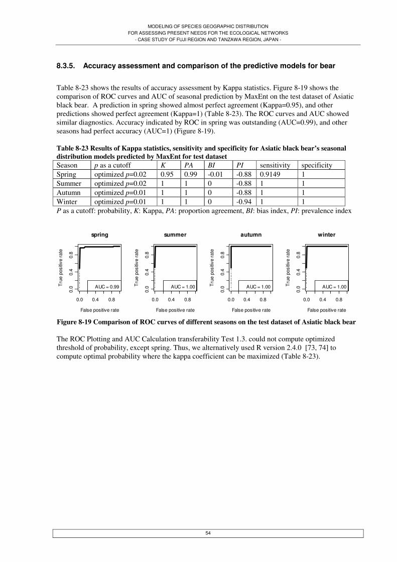
MODELING OF SPECIES GEOGRAPHIC DISTRIBUTION FOR ASSESSING PRESENT NEEDS FOR THE ECOLOGICAL NETWORKS
- CASE STUDY OF FUJI REGION AND TANZAWA REGION, JAPAN -
54
8.3.5. Accuracy assessment and comparison of the predictive models for bear
Table 8-23 shows the results of accuracy assessment by Kappa statistics. Figure 8-19 shows the comparison of ROC curves and AUC of seasonal prediction by MaxEnt on the test dataset of Asiatic black bear. A prediction in spring showed almost perfect agreement (Kappa=0.95), and other predictions showed perfect agreement (Kappa=1) (Table 8-23). The ROC curves and AUC showed similar diagnostics. Accuracy indicated by ROC in spring was outstanding (AUC=0.99), and other seasons had perfect accuracy (AUC=1) (Figure 8-19). Table 8-23 Results of Kappa statistics, sensitivity and specificity for Asiatic black bear’s seasonal distribution models predicted by MaxEnt for test dataset Season p as a cutoff K PA BI PI sensitivity specificity Spring optimized p=0.02 0.95 0.99 -0.01 -0.88 0.9149 1 Summer optimized p=0.02 1 1 0 -0.88 1 1 Autumn optimized p=0.01 1 1 0 -0.88 1 1 Winter optimized p=0.01 1 1 0 -0.94 1 1 P as a cutoff: probability, K: Kappa, PA: proportion agreement, BI: bias index, PI: prevalence index
The ROC Plotting and AUC Calculation transferability Test 1.3. could not compute optimized threshold of probability, except spring. Thus, we alternatively used R version 2.4.0 [73, 74] to compute optimal probability where the kappa coefficient can be maximized (Table 8-23).
spring
False positive rate
Tru
e po
sitiv
e ra
te
0.0 0.4 0.8
0.0
0.4
0.8
AUC = 0.99
summer
False positive rate
Tru
e po
sitiv
e ra
te
0.0 0.4 0.8
0.0
0.4
0.8
AUC = 1.00
autumn
False positive rate
Tru
e po
sitiv
e ra
te
0.0 0.4 0.8
0.0
0.4
0.8
AUC = 1.00
winter
False positive rate
Tru
e po
sitiv
e ra
te
0.0 0.4 0.80.
00.
40.
8
AUC = 1.00
Figure 8-19 Comparison of ROC curves of different seasons on the test dataset of Asiatic black bear

MODELING OF SPECIES GEOGRAPHIC DISTRIBUTION FOR ASSESSING PRESENT NEEDS FOR THE ECOLOGICAL NETWORKS
- CASE STUDY OF FUJI REGION AND TANZAWA REGION, JAPAN -
55
8.4. Japanese serow’s distribution
8.4.1. Screening of predictors for Japanese serow
(a) Analysis of predictors grouped by presence and absence records for Japanese serow’s train data From grouped boxplots of each environmental predictor by two samples of presence and absence of Japanese serow’s records (Figure 13-14 in Appendix 6-2-6: Grouped boxplots of each environmental predictor by two samples of presence and absence of Japanese serow’s records), following were observed. For the altitude, the median, the h-spread looked separated well. However the range between upper and lower whisker did not seem so. A threshold to differentiate h-spread of absence and presence samples was around 500 m. Serow occupied an elevational range of approximately 200~1300 m. For slope, the median and h-spread looked separated but the range between upper and lower whisker did not seem so. A threshold to differentiate h-spread was around 18 . Serow was found in 0 ~60 of slope. The annual mean precipitation did not look a good predictor, because only the median looked separated but the h-spread and range of whisker in absence samples covered the ones of presence samples much. The annual min. temperature looks like a good predictor; the median and the h-spread looked separated well, but there were overlaps in the range between lower and upper whisker. A threshold to differentiate h-spread seemed to be around 7 . The annual max. temperature seemed to be a good predictor as well; the median and h-spread looked separated well, but separation in the range between upper and lower whisker did not look good. A threshold to differentiate h-spread was seen around 17 . Serow was found in 2~10 for annual min. temperature and 12~19 for annual max. tempearture. The distance to all roads did not look like a good predictor; though the median looked separated, both of the h-spread and the range of upper and lower whisker of the presence records covered the ones of absence records. The distance to highways showed that the presence records were concentrated in the places close to the highways; the distance to highways did not exceed 15 km. However the distribution of absence and presence records were overlapped therefore as a predictor it was not considered good. The distance to general roads did not look like a good predictor; though the median was seen separated, the h-spread and the whisker range seemed to be overlapped. The distance to (small) paths and stone steps seemed to be a good predictor. The median and the h-spread looked separated well, but the range between upper and lower whisker did not look separated. A threshold to differentiate h-spread was around 3 km. The distance to wide roads did not look a good predictor; though the median seemed to be separated, the h-spread, and upper and lower whisker seemed to be overlapped. However the serow’s presence records were located to close to the wide roads; the distance to wide roads did not exceed 11 km. The distance to narrow roads looked a moderate predictor; the median looked separated; h-spread looked almost separated with some overlaps from 80 m to 100 m; the range between upper and lower whisker of presence records included the one of absence records. Serow habited 0~9.5 km from paths and stone steps, and 0~600 m from narrow roads. The distance to river streams did not look a good predictor because the distribution of absence records covered the one of presence records. The NDVI also did not look like a good predictor; the median and h-spread were almost same. As a summary, from boxplots, following variables were considered to be potentially excellent for predicting serow’s occurrences: altitude, slope, annual min. temperature, annual max. temperature, and distance to (small) paths and stone steps. Following was considered to be potentially good:

MODELING OF SPECIES GEOGRAPHIC DISTRIBUTION FOR ASSESSING PRESENT NEEDS FOR THE ECOLOGICAL NETWORKS
- CASE STUDY OF FUJI REGION AND TANZAWA REGION, JAPAN -
56
distance to narrow roads. Following were considered to be moderate: distance to all roads, and distance to general roads. The annual mean precipitation, distance to highways, distance to wide roads, distance to rivers, and NDVI were not expected to be good predictors. (b) Jackknife test of variable importance for Japanese serow’s train data
Figure 8-20 Jackknife analysis by the experimental model of MaxEnt with all environmental variables for Japanese serow’s train data The jackknife analysis of the experimental model for Japanese serow (Figure 8-20) indicated that distance to river streams and distance to general roads, annual precipitation, and NDVI were relatively most important variables among a set of variables. It also shows that distance to highways, annual min. temperature, and annual max. temperature were very important but variables such as slope and distance to narrow roads were not such important compared to the above mentioned variables. Other variables such as vegetation cover type, distance to wide roads, distance to small streets, distance to all roads, and altitude were not important with only that variable. (c) Vegetation cover types for Japanese serow’s train data Table 8-24 Cross-classification table of 4 vegetation cover types between serow’s absence and presence records
Table 8-24 shows a cross-classification table of proportion for 4 vegetation cover types between Japanese serow’s absence and presence records. The most frequent place where the Japanese serow’s presence was recorded was the low country (32 %). It was also observed in montane zone (29 %) and planted forest (27 %). The Japanese serow’s absence records were plotted in others most often (64 %). The Pearson's Chi-squared test indicated significance difference among two these samples (X2 = 95.1637, d.f. = 3, p < 2.2e-16).
montane zone low country plantation others Absent (%) 3 18 15 64 Present (%) 29 32 27 11
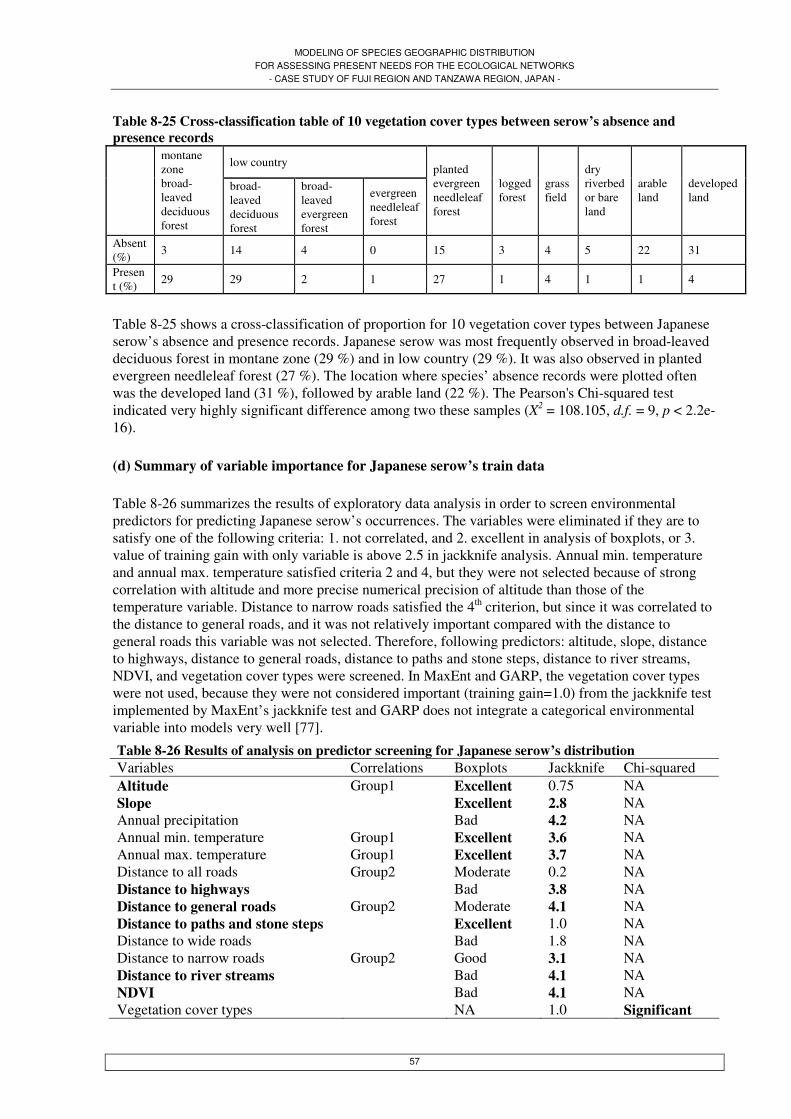
MODELING OF SPECIES GEOGRAPHIC DISTRIBUTION FOR ASSESSING PRESENT NEEDS FOR THE ECOLOGICAL NETWORKS
- CASE STUDY OF FUJI REGION AND TANZAWA REGION, JAPAN -
57
Table 8-25 Cross-classification table of 10 vegetation cover types between serow’s absence and presence records
low country
montane zone broad-leaved deciduous forest
broad-leaved deciduous forest
broad-leaved evergreen forest
evergreen needleleaf forest
planted evergreen needleleaf forest
logged forest
grass field
dry riverbed or bare land
arable land
developed land
Absent (%) 3 14 4 0 15 3 4 5 22 31
Present (%) 29 29 2 1 27 1 4 1 1 4
Table 8-25 shows a cross-classification of proportion for 10 vegetation cover types between Japanese serow’s absence and presence records. Japanese serow was most frequently observed in broad-leaved deciduous forest in montane zone (29 %) and in low country (29 %). It was also observed in planted evergreen needleleaf forest (27 %). The location where species’ absence records were plotted often was the developed land (31 %), followed by arable land (22 %). The Pearson's Chi-squared test indicated very highly significant difference among two these samples (X2 = 108.105, d.f. = 9, p < 2.2e-16). (d) Summary of variable importance for Japanese serow’s train data Table 8-26 summarizes the results of exploratory data analysis in order to screen environmental predictors for predicting Japanese serow’s occurrences. The variables were eliminated if they are to satisfy one of the following criteria: 1. not correlated, and 2. excellent in analysis of boxplots, or 3. value of training gain with only variable is above 2.5 in jackknife analysis. Annual min. temperature and annual max. temperature satisfied criteria 2 and 4, but they were not selected because of strong correlation with altitude and more precise numerical precision of altitude than those of the temperature variable. Distance to narrow roads satisfied the 4th criterion, but since it was correlated to the distance to general roads, and it was not relatively important compared with the distance to general roads this variable was not selected. Therefore, following predictors: altitude, slope, distance to highways, distance to general roads, distance to paths and stone steps, distance to river streams, NDVI, and vegetation cover types were screened. In MaxEnt and GARP, the vegetation cover types were not used, because they were not considered important (training gain=1.0) from the jackknife test implemented by MaxEnt’s jackknife test and GARP does not integrate a categorical environmental variable into models very well [77].
Table 8-26 Results of analysis on predictor screening for Japanese serow’s distribution Variables Correlations Boxplots Jackknife Chi-squared Altitude Group1 Excellent 0.75 NA Slope Excellent 2.8 NA Annual precipitation Bad 4.2 NA Annual min. temperature Group1 Excellent 3.6 NA Annual max. temperature Group1 Excellent 3.7 NA Distance to all roads Group2 Moderate 0.2 NA Distance to highways Bad 3.8 NA Distance to general roads Group2 Moderate 4.1 NA Distance to paths and stone steps Excellent 1.0 NA Distance to wide roads Bad 1.8 NA Distance to narrow roads Group2 Good 3.1 NA Distance to river streams Bad 4.1 NA NDVI Bad 4.1 NA Vegetation cover types NA 1.0 Significant

MODELING OF SPECIES GEOGRAPHIC DISTRIBUTION FOR ASSESSING PRESENT NEEDS FOR THE ECOLOGICAL NETWORKS
- CASE STUDY OF FUJI REGION AND TANZAWA REGION, JAPAN -
58
8.4.2. Predictive equation from Generalized Linear Model for Japanese serow
(a) Comparison of Generalized Linear Models for Japanese serow We carried out a forward stepwise logistic regression of the training distribution data of Japanese serow with altitude (code: DEM), slope, annual min. temperature (code: Tmin), 4 vegetation cover types (code: Veg1), and 10 vegetation cover types (code: Veg2). The models were compared by AIC (Akaike’s An Information Criterion), Adjusted D2 (Adj. D2), AUC, sensitivity, specificity, and significance of the probability (Pr(>|z|)) for coefficients. (Table 8-27) Table 8-27 Comparison of logistic regression models for predicting Japanese serow AIC Adj. D2 AUC Sensitivity Specificity Significance code DEM 210 0.48 0.92 0.91 0.88 *** Sqrt(DEM) 186 0.54 0.93 0.95 0.87 *** Slope 305 0.24 0.81 0.71 0.80 *** Tmin 189 0.54 0.94 0.99 0.88 *** Veg1 230 0.27 0.80 0.89 0.64 No mark~*** Veg2 292 0.32 0.84 0.87 0.68 No mark~*** Sqrt(DEM) + Veg2 194 0.57 0.93 0.93 0.88 No mark~*** Sqrt(DEM) + Veg1 187 0.55 0.93 0.92 0.88 No mark~*** Sqrt(DEM) + Slope 177 0.57 0.94 0.93 0.85 ** ~ *** Tmin + Veg2 186 0.59 0.94 0.94 0.89 No mark~*** Tmin + Veg1 183 0.57 0.94 0.96 0.90 ** ~ *** Tmin + Slope 177 0.57 0.94 0.93 0.85 ** ~ *** Sqrt(DEM) * Slope 179 0.57 0.94 0.93 0.85 No mark~*** Tmin * Slope 177 0.58 0.95 0.94 0.89 No mark~*** Significance codes of Pr(>|z|) for predictors’ coefficients: 0 '***' 0.001 '**' 0.01 '*' 0.05 '.' 0.1 ' ' 1 Compared to altitude (code: DEM), square root of altitude (code: Sqrt(DEM)) was a better predictor; AIC is much less, 54 % of total variance was explained while altitude explained 48 % of total variance. As a single predictor, square root of altitude (code: Sqrt(DEM)) and annual min. temperature (code: Tmin) performed similarly (AIC, AUC, sensitivity, specificity and significance of coefficients were approximately same, Adjusted D2 was same). As a single predictor, slope (code: Slope), 4 vegetation cover types (code: Veg1), and 10 vegetation cover types (Code: Veg2) were not superior to the DEM and annual min. temperature. Since DEM and annual min. temperature were correlated (See Table 8-1 and Table 8-2), it was considered reasonable to use either of them. Therefore models by another predictor (Slope, Veg 1, or Veg 2) with one of the predictors (Sqrt(DEM) or Tmin) without interaction were built. The two models predicted by (1) Sqrt(DEM) and Slope and by (2) Tmin and Slope performed best. (All indices scored same.) Because of two practical reasons, the model (1) was chosen as the best logistic regression model for presence/absence records of Japanese serow. First, the precision of altitude is much more precise than temperature data. Secondly the resolution of the original environmental maps was more accurate in altitude than in temperature data; this is important considering the needs of extrapolation of the equation of logistic regression model for the study area. The models by two predictors with interaction were also created but they did not improve the performance.

MODELING OF SPECIES GEOGRAPHIC DISTRIBUTION FOR ASSESSING PRESENT NEEDS FOR THE ECOLOGICAL NETWORKS
- CASE STUDY OF FUJI REGION AND TANZAWA REGION, JAPAN -
59
(b) The best logistic regression model for Japanese serow’s prediction The best logistic regression model was considered to be predicted by square root of DEM and slope without interaction, derived from the following predictive equation:
( )( ) 21 *0.26478759 * 0.04024136 0-5.91785431/log xxpp ++=− (Equation 10) where x1 is slope (˚) and x2 is square root of altitude (m2);
)1/( 2121 *0.26478759 * 0.04024136 0-5.9178543*0.26478759 * 0.04024136 0-5.9178543 xxxx eep ++++ += (Equation 11)
where p is the probability of Japanese serow’s occurrences. Deviance of residuals and coefficients of the best model are summarized in Table 8-28 and Table 8-29. Table 8-28 Deviance of residuals of the best logistic regression model for presence/absence records of Japanese serow Min 1Q Median 3Q Max -3.13702 -0.22224 -0.07618 0.51673 2.04681 Table 8-29 Coefficients of the best logistic regression model for presence/absence records of Japanese serow Estimate Std. Error z value Pr(>|z|) (Intercept) -5.91785 0.76429 -7.743 9.71e-15 *** Slope 0.04024 0.01282 3.138 0.0017 ** Square root of altitude 0.26479 0.03459 7.655 1.93e-14 *** Signif. codes: 0 '***' 0.001 '**' 0.01 '*' 0.05 '.' 0.1 ' ' 1
0 50 100 150 200 250
0.0
0.2
0.4
0.6
0.8
1.0
sorted sample number
prob
abili
ty
fitted probability
Success of logistic model
mean probability
midpoint||||||||||||||||||||||||||||||||||||||||||||||||||||||||||||||||||||||||||||||||||||||||||||||||
|
||||||||
|
||||
|
|||||||
||
|
|||
||||
|
|
|
||||||
||
|
|||
|||
|
|
|||||||
|
||||||||||
|
||||||
|
||||||||||||||||||||||||||||||||||||
|
||||||
|
||||||||||||||||||||
|
||||
|
|||
|
|||||
|
|||||||
|
|||||||
|
|||||||||||
|
|||||
FALSE Samples
TRUE Samples
Model: pa ~ serowdata$slope + sqrt(serowdata$dem)AIC: 177
Null deviance: 398
50 100 150 200 250
0.0
0.2
0.4
0.6
0.8
1.0
prob
abili
ty o
f cha
nge
threshold = 0.5
crossover
fitted probability of change
||||||||||||||||||||||||||||||||||||||||||||||||||||||||||||||||||||||||||||||||||||||||||||||||
|
||||||||
|
||||
|
|||||||
||
|
|||
||||
|
|
|
||||||
||
|
|||
|||
|
|
|||||||
|
||||||||||
|
||||||
|
||||||||||||||||||||||||||||||||||||
|
||||||
|
||||||||||||||||||||
|
||||
|
|||
|
|||||
|
|||||||
|
|||||||
|
|||||||||||
|
|||||
True negatives: 123 False positives: 21
True positives: 133False negatives: 10
Model success
Sensitivity: 0.9301 ; Specificity: 0.8542
Figure 8-21 Visualization of the best logistic regression model and model success for predicting Japanese serow’s distribution (left: success of logistic regression model, right: model success with sensitivity and specificity) Figure 8-21 shows the visualization of the best logistic regression model. The coefficients of predictors were very highly or highly significant (p=9.71e-15 for intercept, p= 0.0017 for slope, and p = 1.93e-14 for square root of altitude); 57 % of total variance was explained by this logistic regression model (Adjusted D2: 0.57); AIC is lowest among others (AIC=177). At a threshold of 0.5, both of sensitivity and specificity were excellent or very good (sensitivity=0.93 and specificity=0.85), and AUC was excellent (=0.94).

MODELING OF SPECIES GEOGRAPHIC DISTRIBUTION FOR ASSESSING PRESENT NEEDS FOR THE ECOLOGICAL NETWORKS
- CASE STUDY OF FUJI REGION AND TANZAWA REGION, JAPAN -
60
8.4.3. Predictor variable importance for Japanese serow
Figure 8-22 Jackknife test of variable importance for the Japanese serow’s training dataset The Figure 8-22 shows the results of the MaxEnt’s jackknife test of variable importance for Japanese serow. The environmental variable with highest gain when used in isolation is altitude, which therefore appears to have the most useful information by itself. The environmental variable that decreases the gain the most when it is omitted is also altitude, which therefore appears to have the most information that isn't present in the other variables. The secondly important factor was distance to paths and stone steps, followed by slope. (See Figure 13-16 in Appendix 6-3-2. Response curves of MaxEnt for predicting Japanese serow.)

MODELING OF SPECIES GEOGRAPHIC DISTRIBUTION FOR ASSESSING PRESENT NEEDS FOR THE ECOLOGICAL NETWORKS
- CASE STUDY OF FUJI REGION AND TANZAWA REGION, JAPAN -
61
8.4.4. Predictive distribution maps for Japanese serow
Figure 8-23 Probabilistic predictive maps of Japanese serow’s distribution by MaxEnt, GARP, and GLM

MODELING OF SPECIES GEOGRAPHIC DISTRIBUTION FOR ASSESSING PRESENT NEEDS FOR THE ECOLOGICAL NETWORKS
- CASE STUDY OF FUJI REGION AND TANZAWA REGION, JAPAN -
62
Figure 8-23 shows probabilistic predictive maps for Japanese serow predicted by three algorithms. Three predicted maps showed very different patterns in this case. For example, prediction by GLM indicated the species’ appearance in the South Alps region, but other two models did not. All models predicted the occurrence of Japanese serow in Tanzawa region. MaxEnt did not predict any presence around Fuji region, but GARP and GLM predicted occurrence there though the extent was different. The GLM predicted species’ occurrence in Hakone volcano and in Izu Peninsula where are the part of Fuji-Hakone-Izu National Park. (Refer to Section 7.1: Study area for name of locations.) For comparison purposes the optimum threshold value was used as a cutoff of the probabilistic predictive maps (Figure 8-24). The optimum p value corresponds to the optimized p in Table 8-30 and Table 8-31.
Figure 8-24 Predictive maps of Japanese serow by different modeling algorithms with optimized p value as cutoff Using the cutoff value, the prediction by MaxEnt showed more species’ presence close to South Alps region, but compared to GLM’s, still the difference in patterns was clear. GLM predicted more presence in this region. The area ranged from west part of Kanagawa Prefecture to the Fuji region in West direction and to Hakone region in South direction, the species were predicted present by GARP and MaxEnt. In this area, these two algorithms showed similar patterns. However, the map by GLM showed isolation or fragmented area between Fuji-Tanzawa regions and Hakone volcano. Both of MaxEnt and GLM predicted species’ presence in Izu Peninsula.
8.4.5. Accuracy assessment and comparison of the predictive models for Japanese serow
Table 8-30 and Table 8-31 show the results of accuracy assessment by Kappa statistics and ROC curves. Figure 8-25 shows the comparison of ROC curves of MaxEnt, GARP, GLMs on the train and test dataset of Japanese serow. In general the score of indices was better at an optimized probability than at a threshold of probability of 0.5 except a case of GLM for the test data (Table 8-30). For both of the test data and the train data, AUC was outstanding (AUC>0.9) and the prediction was very highly significant (p<0.0001) (Table 8-31). From visual inspection of ROC curves, the difference between three modeling algorithms was not clear (Figure 8-25). For Japanese serow’s prediction,

MODELING OF SPECIES GEOGRAPHIC DISTRIBUTION FOR ASSESSING PRESENT NEEDS FOR THE ECOLOGICAL NETWORKS
- CASE STUDY OF FUJI REGION AND TANZAWA REGION, JAPAN -
63
GARP was the best algorithm which fitted the distribution; all indices were perfect at a threshold of probability of 0.5. Table 8-30 Results of Kappa statistics, sensitivity, and specificity for Japanese serow’s distribution models predicted by MaxEnt, GARP, and GLMs, for test dataset and train dataset respectively algorithm p as a cutoff K PA BI PI sensitivity specificity
p=0.5 0.56 0.78 -0.22 -0.22 0.5625 1 MaxEnt optimized p=0.04 0.88 0.94 0 0 0.9375 0.9375
GARP p=0.5 1 1 0 0 1 1 p=0.5 0.81 0.91 0.03 0.03 0.9375 0.875
Test data
GLM optimized p=0.63 0.75 0.88 0 0 0.875 0.875 p=0.5 0.55 0.78 -0.21 -0.21 0.5664 0.9861 MaxEnt optimized p=0.03 0.87 0.93 0 -0.01 0.9301 0.9375 p=0.5 0.9 0.95 0.04 0.04 0.5664 0.9861 GARP optimized p=0.80 0.93 0.97 0.03 0.02 0.993 0.9375 p=0.5 0.78 0.89 0.04 0.03 0.9301 0.8542
Train data
GLM optimized p=0.52 0.81 0.91 0.02 0.02 0.9301 0.8819
P as a cutoff: probability, K: Kappa, PA: proportion agreement, BI: bias index, PI: prevalence index Table 8-31 Results of Receiver Operating Characteristic (ROC) curves for Japanese serow’s distribution models predicted by MaxEnt, GARP, and GLMs, for test dataset and train dataset respectively
The ROC Plotting and AUC Calculation transferability Test 1.3. failed to compute indices concerning standard bootstrap method in case of GARP’s prediction for test data (Table 8-31). (a) test dataset
(b) train dataset
Figure 8-25 Comparison of ROC curves of MaxEnt, GARP, GLMs on the test and the train dataset of Japanese serow
AUC SE z p lower upper MaxEnt 0.98 0.0203 13.803 <0.0001 0.94 1.02 GARP 1.00
Test data
GLMs 0.98 0.0204 13.586 <0.0001 0.94 1.02 MaxEnt 0.98 0.0074 37.428 <0.0001 0.96 0.99 GARP 0.97 0.0107 25.049 <0.0001 0.95 0.99
Train data
GLMs 0.94 0.0160 14.858 <0.0001 0.91 0.97

MODELING OF SPECIES GEOGRAPHIC DISTRIBUTION FOR ASSESSING PRESENT NEEDS FOR THE ECOLOGICAL NETWORKS
- CASE STUDY OF FUJI REGION AND TANZAWA REGION, JAPAN -
64
8.5. Estimated local population of potential suitable habitat patches
8.5.1. Result of estimated local population for Asiatic black bear and analysis
Figure 8-26 Potential suitable habitat patches for Asiatic black bear predicted by MaxEnt Table 8-32 Population of Asiatic black bear estimated by area in km2 and population density Location Area (km2) Estimated population Mt. Aitaka 30 5~9 Fuji and Tanzawa regions 340 51~102 South Alps region 1066 160~320 Mt. Kenashi 28 4~8 Izu Peninsula 28 4~8 Hakone 37 6~11
Figure 8-27 Potential suitable habitat patches for Asiatic black bear with other information

MODELING OF SPECIES GEOGRAPHIC DISTRIBUTION FOR ASSESSING PRESENT NEEDS FOR THE ECOLOGICAL NETWORKS
- CASE STUDY OF FUJI REGION AND TANZAWA REGION, JAPAN -
65
Figure 8-26 shows the potential suitable habitat patches for Asiatic black bear predicted by MaxEnt, which was the most accurate among three algorithms. The grouped patches were considered to represent the metapopulation or sub-metapopulation of the Asiatic black bear. Population of each metapopulation or sub-metapopulation was estimated as indicated in Table 8-32. These results showed that there are six main patches in the study area. In the South Alps region, the estimated population was from 160 to 320 (Table 8-32). The map showed a united large habitat (1066 km2) in this region. It is known that Fuji metapopulation of the Asiatic black bear consist of four sub-metapopulations: Mt. Fuji, Mt. Aitaka, Mt. Furo, and Mt. Kenashi [32] (See Appendix 3-2: Asiatic black bear in Fuji region). As for the area of our interest, a linear corridor seemed to exist to connect two metapopulations: the Fuji metapopulation and the Tanzawa metapopulation (Figure 8-26). Estimated population was from 51 to 102 (Table 8-32). From the map, it seemed that the connected patch contained the Tanzawa metapopulation, sub-metapopulation of Mt. Fuji, and Mt. Furo. However, the predictive map showed that Mt.Aitaka and Mt. Kenashi were isolated from other sub-metapopulations. The estimated population in Mt. Kenashi was from 4 to 8; in Mt. Aitaka it was from 5 to 9 (Table 8-32). The predictive map also showed species’ suitable habitat patches in Izu Peninsula and Hakone volcano. Compared to the habitat in South Alps and the one in Fuji-Tanzawa, the habitats in this area seemed to be small and fragmented. Estimated population in Izu Peninsula was from 4 to 8 and in Hakone volcano it was from 6 to 11 (Table 8-32). Figure 8-27 showed basically the same information as Figure 8-38, but it contains the boundaries of Fuji-Hakone-Izu National Park and Tanzawa Quasi-national Park, and environmental predictors used for bear in MaxEnt. Figure 8-27 showed that the potential suitable habitat patches were geographically distant from the wide roads and paths and stone steps. The bear’s predicted distribution was almost covered by the National Park and Quasi-national Park. However, the habitats around Mt. Aitaka were not covered by the Fuji-Hakone-Izu National Park. Also, the patch which consists of a linear corridor between Fuji and Tanzawa was not covered by the Fuji-Hakone-Izu National Park and Tanzawa Quasi-national Park. In general, the predicted distribution of the bear ranged from 600 to 1800 m both in South Alps and Fuji-Tanzawa patch, but around Mt. Fuji, it even predicted the presence around the top of the mountain (3742 m). Also, the predicted habitat was located mainly in the montane zone. (See Appendix 4-1: Maps of environmental variables.)

MODELING OF SPECIES GEOGRAPHIC DISTRIBUTION FOR ASSESSING PRESENT NEEDS FOR THE ECOLOGICAL NETWORKS
- CASE STUDY OF FUJI REGION AND TANZAWA REGION, JAPAN -
66
8.5.2. Result of estimated local population for Japanese serow and analysis
Figure 8-28 Potential suitable habitat patches for Japanese serow predicted by GARP Table 8-33 Population of Japanese serow estimated by area in km2 and population density Location Area (km2) Estimated population Fuji and Tanzawa regions 1581 < 1581 South Alps region 537 < 537
Figure 8-29 Potential suitable habitat patches for Japanese serow with other information

MODELING OF SPECIES GEOGRAPHIC DISTRIBUTION FOR ASSESSING PRESENT NEEDS FOR THE ECOLOGICAL NETWORKS
- CASE STUDY OF FUJI REGION AND TANZAWA REGION, JAPAN -
67
Figure 8-28 shows the potential suitable habitat patches for Japanese serow predicted by GARP, which was the most accurate among three algorithms. The patches were grouped into two metapopulation: the area of interest and others. Population was estimated as indicated in Table 8-33. As for the area of interest, the predictive map showed a large connected habitat (1581 km2) which covered Tanzawa region, Hakone region and part of Fuji region. Estimated population was under 1581 (Table 8-33). This large patch in Tanzawa, Hakone, and Fuji elevational range was from 250 m to 1800 m. The habitat in Fuji region was not predicted in higher altitude of Mt. Fuji (1800 m to 3742 m) but it seemed to surround Mt. Fuji and was concentrated around the lower part of the mountain. It ranged in the slope of 16 to 30 in general, but for some part it even occurred in gentle slope of 0 to 15 as well. (See Appendix 4-1: Maps of environmental variables.) The patches in South Alps were 537 km2 and the estimated population was under 537 (Table 8-33). They looked somewhat patchy, but their habitats were not distant each other. The suitable habitat surrounded the mountains in South Alps region. It showed serow’s presence in the slope approximately from 16 to 30 and in lower altitude from 250 m to 600 m. (See Appendix 4-1: Maps of environmental variables.) Figure 8-29 showed basically the same information as Figure 8-28, but it contains the boundaries of Fuji-Hakone-Izu National Park and Tanzawa Quasi-national Park, and environmental predictors used for Japanese serow in GARP. The Hakone National Park and Tanzawa Quasi-national Park were fully covered by the suitable habitat, but only small part of the Fuji National Park was covered by that patch. In general, the potential suitable habitat was close to the highways; it looked the habitat was located along the highways. However the suitable habitat was distant from the paths and stone steps.

MODELING OF SPECIES GEOGRAPHIC DISTRIBUTION FOR ASSESSING PRESENT NEEDS FOR THE ECOLOGICAL NETWORKS
- CASE STUDY OF FUJI REGION AND TANZAWA REGION, JAPAN -
68
9. Discussion
9.1. Different performance of modeling algorithms
Our analysis revealed that the performance of the modeling algorithms differs in 1) kinds of species, 2) probability as cutoff, and 3) test data or train data. (a) Kinds of species As for the kinds of species, for the Asiatic black bear, MaxEnt algorithm produced the most accurate map among three chosen algorithms (Kappa=0.75 at p=0.005 and AUC=0.95), and for the Japanese serow, GARP algorithm produced the most accurate map among three (Kappa=1 at p=0.5 and AUC=1.00). Generalized Linear Model (logistic regression model) did not perform better than the others for these two species (Kappa=0.69 and AUC=0.95 for bear and Kappa=0.75 and AUC=0.98 for serow). These results suggest that the performance of modeling algorithm depends on the kinds of species distribution. Our results confirm the findings of Segurado et al. (2004) [110]. It also supports our first hypothesis: “There is a difference between the accuracy of the maps generated by different modeling algorithms.” To the author’s knowledge, this is the first attempt to investigate appropriate modeling methods for the chosen species: Asiatic black bear and Japanese serow. A suggestion is made that the MaxEnt algorithm may be useful to model Asiatic black bear’s distribution, and the GARP algorithm may be appropriate to model the Japanese serow’s distribution. However the logistic regression model is certainly not a bad choice; their accuracy was at least substantial in kappa statistics, and outstanding in AUC. (b) Probability as cutoff In general, indices, such as kappa coefficient, proportion agreement, bias index, prevalence index, sensitivity and specificity, showed better score at an optimum cutoff [84, 101] than the ones at cutoff probability of 0.5. What does this result indicate? First of all, the above-mentioned indices are highly dependent of a threshold value [84, 96, 111]. Bonn (2001) [84] stated that but even when optimum probability is examined, possible evaluation of habitat model transfers based on confusion matrices might lead to seemingly unsatisfactory results, merely because of differences for optimum p within the compared data sets. However, this opinion is based on the transferability of the habitat models. At the current moment, no validation technique was superior in all circumstances. Our result indicates that the accuracy of the models can be maximized by implementing optimum cutoff threshold. On the other hand, ROC plots and AUC have their own advantage that they are independent from the threshold value probability and AUC provides a single quantitative index of the diagnostic accuracy of the model [102]. Therefore, we recommend employing multi-evaluation techniques, such as kappa statistics at an optimum cutoff value of probability, ROC plots, and AUC. (c) Test data or train data In general, the accuracy of the test data was lower than the one of the train data. For the Japanese serow, there was not a big difference in the performance between test and train data, but for the Asiatic black bear, the accuracy differed dramatically. For the train dataset of the bear, kappa coefficient was almost perfect (Kappa 0.98) and AUC was outstanding (AUC=1.00) for all modeling algorithms. Contrary to this, the accuracy of the test data of bear showed significant

MODELING OF SPECIES GEOGRAPHIC DISTRIBUTION FOR ASSESSING PRESENT NEEDS FOR THE ECOLOGICAL NETWORKS
- CASE STUDY OF FUJI REGION AND TANZAWA REGION, JAPAN -
69
difference (Kappa=0.75 for MaxEnt, Kappa=0 for GARP, Kappa=0.69 for GLM, AUC=0.95 for MaxEnt and GLM, and AUC=0.5 for GARP). One reason may be explained by the method for preparing a test dataset and a train dataset. For the Japanese serow’s dataset, we adopted split-sample approach� For the bear’s annual average distribution, we used an independent dataset and attempted to build predictive models by the test dataset in South Alps metapopulation and evaluate the models by the train dataset in Fuji metapopulation. Our results suggest that the above two metapopulations have different habitat preference. Another reason for this result may be due to the characteristics of GARP. There was a considerable gap in the GARP prediction between test dataset (Kappa=0 and AUC=0.5) and for train dataset (Kappa=1 and AUC=1.00). We attribute this issue to the behavior of GARP algorithm, “overestimation”. The same problem is reported by Phillips et al. (2006) [77] and García (2006) [97]. On the other hand, our analysis revealed that the optimum probability of bear’s occurrences were much lower in Fuji metapopulation (test data) than in South Alps metapopulation (train data) (for test data p=0.005 by MaxEnt, p=0.033 for GLM; for train data p=0.02 for MaxEnt, p=0.053 for GARP, and p=0.613 for GLM). We attribute this to that the suitability of habitat is lower in Fuji metapopulation than in South Alps metapopulation. We suggest the failure of GARP’s prediction for bear’s test data is due to the GARP’s capacity to detect low probability of species’ occurrences. GARP produces binominal predictive maps (0 or 1), so we averaged 10 best subsets to make a probabilistic map. As a result the probabilistic predictive map for bear had discrete prediction with only 10 classes (0.0, 0.1, 0.2,…., 0.7, 0.8, 0.9, 1.0). We suggest that the precision of a GARP’s predictive map is not sufficient for predicting extremely low probability. Phillips et al. (2006) [77] also pointed out that, in comparison with GARP, the important advantage of MaxEnt was the continuous precise prediction.
9.2. Controlling factors of target species’ survival
(a) Asiatic black bear (annual average distribution) 1. Habitat selection From our boxplots analysis, altitude, annual min. temperature, annual max. temperature, distance to wide roads, and distance to paths and stone steps, slope, and distance to highways showed good separation between bear’s presence and absence records. The range of elevation belongs to montane zone. Montane regions generally have cooler temperatures than the adjacent lowland regions. Good separation in temperature data between absence and presence confirm it. To our knowledge, this is the first attempt to investigate bear’s habitat or limiting factors in their numerical range; especially the bear’s habitat analysis in relation with slope and distance to roads has not been carried out. Our result suggests that bear prefers habitat with slope to some extent. As for variables concerning roads, boxplots of presence records were distributed in more distant locations than the absence records were. Our results indicate that bear prefers area geographically distant from roads, seemingly to avoid roads. Contrary to above variables, annual precipitation, distance to river streams, and NDVI did not show good separation between absence and presence records. On the other hand, the Pearson's Chi-squared test proved a very highly significant difference between bear’s absence and presence records for regrouped vegetation cover types (for regrouped 5 vegetation cover types: X2=949, d.f. = 4, p < 2.2e-16 and for 14 regrouped vegetation cover types: X2=1164, d.f. = 13, p < 2.2e-16). A cross-classification of proportion for 5 vegetation cover types showed that most of the presence records were observed in the montane zone (79 %), but some were present in the subalpine zone (4 %) and in planted forest as well (4 %). Another cross-classification of proportion for regrouped 14 vegetation cover types revealed that broad-leaved deciduous forest in the montane zone (65 %) was the most frequent place where the bear is found, followed by evergreen needleleaf forest in montane zone (14 %), logged forest (9 %), and planted evergreen needleleaf forest (3 %). It is believed that bear’s survival depends on good amount and good quality of broad-leaved deciduous forest in montane zone [26, 54, 112]. Our results confirmed that bear’s major habitats belong to that category, but some inhabit evergreen needleleaf forest in montane zone as well. Habitat loss are reported throughout

MODELING OF SPECIES GEOGRAPHIC DISTRIBUTION FOR ASSESSING PRESENT NEEDS FOR THE ECOLOGICAL NETWORKS
- CASE STUDY OF FUJI REGION AND TANZAWA REGION, JAPAN -
70
Asiatic black bear range [26]. Our result suggests that lack of food supply from montane broad-leaved forest may influence on bear’s new habitat selection. More investigation on the causes of this phenomenon is expected. 2. Relative importance of variables Our jackknife test by MaxEnt’s final model ranked the distance to paths and stone steps as first, the distance to wide roads as second, the vegetation cover type with 57 classes as third, and altitude as fourth. From the existing literature variable such as altitude [26, 54] and vegetation cover types [26, 37] is known as the important habitat for bear. However this result can be interpreted that the distance to roads are more important than the vegetation cover types or altitude. Till now there was no study for investigating relative importance of altitude, vegetation cover types, and distance to roads for bear’s distribution. Now the question is why it happens. We prepared 6 kinds of predictors concerning distance to roads; which include all roads, highways, general roads, paths and stone steps, wide roads and narrow roads. The paths and stone steps seem most natural roads among a set of data, but this variable was considered the most important predictor among all sets. What it indicates? One possible interpretation is that, considering the variables related to roads represent hidden effect of human disturbance, these results suggest that the human disturbance have a more considerable negative influence on bear’s distribution than it is currently perceived. We suggest even for the paths and stone steps, which look close to nature, the negative impact on the bear’s distribution should not be neglected. (b) Japanese serow 1. Habitat selection From our boxplots analysis, altitude, slope, annual min. temperature, annual max. temperature, distance to paths and stone steps, and distance to narrow roads showed good separation. The range of elevation belonged to low country. Generally the Japanese serow is believed to be found in the montane regions [59], [113]. Our findings give a new insight for the possible vertical distribution of serow. This indicates the different habitat selection according to metapopulation; The presence records was derived from Yamagushi et al. (1998) [33] only in Tanzawa metapopulation of serow. The serow’s preference for temperature in the low country showed much warmer than the one in montane zone. There are existing studies about serow’s habitat selection in relation with altitude [33, 114] and slope [42]. Also a discussion is made on roads [42]. However, to the author’s knowledge this is the first investigation to carry out statistical analysis of serow’s occurrences in relation with distance to roads. Our result suggests that serow prefers steep slope, which is in agreement with Matsumoto (1984) [114]’s findings. As for variables concerning roads, in general, boxplots of presence records were distributed in more distant locations than the absence records were. Our results indicate that serow prefers area geographically distant from roads. In general serow seems to avoid the presence of roads. However, our results showed that this serow’s behavior depends on the type of the roads. For example, serow’s presence localities were closer to highways than the absence localities were. It indicates that serow prefers to habit close to highways. This finding partly supports Nowicki (2001)‘s observation [42] who reported that serow selected steep slopes and areas close to roads. However Nowicki (2001) [42] did not specify the type of roads and numerical range of distance to the roads. The localities near to highways may be suitable habitat because sometimes highways are built up through the mountains and along the highways its favourite habitat, steep slope, exists. We also attributes this habitat selection to competition with Sika deer, which is in agreement with Nowicki (2001) [42]. Our boxplots analysis also revealed that the serow’s absence and presence records are not separated well for the following variables: annual precipitation, distance to wide roads, distance to river streams, and NDVI. On the other hand, the Pearson's Chi-squared test proved a very highly significant difference between serow’s absence and presence records for regrouped vegetation cover types (for regrouped 4 vegetation cover types: X2=95.1637, d.f. = 3, p < 2.2e-16 and for 10 regrouped

MODELING OF SPECIES GEOGRAPHIC DISTRIBUTION FOR ASSESSING PRESENT NEEDS FOR THE ECOLOGICAL NETWORKS
- CASE STUDY OF FUJI REGION AND TANZAWA REGION, JAPAN -
71
vegetation cover types: X2=108.105, d.f. = 9, p < 2.2e-16). A cross-classification table of frequency of 4 vegetation cover types showed that the most frequent place where serow was found was the low country (32 %), followed by montane zone (29 %) and planted forest (27 %). Another cross-classification table of proportion for regrouped 10 vegetation cover types revealed that serow was most frequently observed in broad-leaved deciduous forest in montane zone (29 %) and in low country (29 %), followed by planted evergreen needleleaf forest (27 %). 2. Relative importance of variables Our jackknife test by MaxEnt’s final model ranked altitude as the most important, distance to paths and stone steps as second, slope as third, distance to highways as forth, NDVI as fifth, distance to general roads as sixth, and distance to rivers as seventh. From the existing literature we expected the importance of altitude [33, 114], slope [42] and vegetation cover types ([41], [60], [33]). Thus we consider the MaxEnt’s selection of altitude and slope is reasonable. However vegetation cover types were not selected for any final model. A jackknife of the experimental MaxEnt model revealed that NDVI is much more important than vegetation cover types with 57 classes. To our knowledge this is the first study to investigate the serow’s occurrences in relation with NDVI. As a relevant study, Sone et al. (1999) [43] investigated biomass of food plants and density of Japanese serow; “The density of serows showed positive relationships with the biomass of food plants in summer and winter. This result suggests that the food biomass was one of the important determinant factors in the serow density in winter. [43]” On the other hand, biomass can be estimated by NDVI; Wylie et al. (2002) [115] found good agreement between scaled-up grid based biomass and NDVI derived from Landsat TM with R2 of 0.92-0.94. We suggest the relationship between NDVI and biomass may explain our result. A further study for investigating a mechanism of driving factors is recommended. As for the choice of distance to paths and stone steps, we propose the same interpretation, as the one in a case of bear.
9.3. Seasonality of the Asiatic black bear
We investigated bear’s seasonality based on different seasons. A set of climatic predictors for each season was prepared for this purpose. 1. Habitat selection Our boxplots analysis revealed that generally difference of habitat selection by season was not clear. The result of assessment based on boxplots showed same ranking as the annual average distribution. However winter season showed somewhat different range of distribution. Also, climatic variables showed different range of distribution by season. In a case of vegetation, for all seasons, the Pearson's Chi-squared test proved a very highly significant difference between bear’s absence and presence records for regrouped vegetation cover types (p < 2.2e-16). Piecharts analysis for vegetation cover types by season revealed that bear is mainly found in Carpinus laxiflora, Carpinus tschonoskii, Fagus japonica, Tsuga sieboldii, Carez reinii, Cryptomeria japonica, Chamaecyparis obtusa, Chamaecyparis pisifera and logged forest. The proportion of vegetation cover types was similar in all seasons, especially in summer and in autumn it was pretty similar. The slight change refers to vegetation cover types by season. Based on statistical analysis, an exactly same set of predictors were selected for the summer and autumn as the one for annual averaged distribution by MaxEnt; selected predictors are altitude, distance to paths and stone steps, distance to wide roads, and vegetation cover types with 57 classes. However, for spring and winter, instead of altitude temperature variables were selected (for spring, min. temperature in spring, and for winter max. temperature in winter). It may indicate that in spring

MODELING OF SPECIES GEOGRAPHIC DISTRIBUTION FOR ASSESSING PRESENT NEEDS FOR THE ECOLOGICAL NETWORKS
- CASE STUDY OF FUJI REGION AND TANZAWA REGION, JAPAN -
72
and in winter the temperature controls the bear’s distribution more than the altitude does. It also suggests that temperature limits the bear’s capabilities to survive in these seasons. 2. Relative importance of variables The results of a jackknife test suggest that relative importance of predictors depends on seasons. For instance vegetation is the most important factor for spring and winter but not for other two seasons. Summer and autumn showed similar gain for variable importance; the most important factors are related to the distance to the roads. Except a case of maximum temperature in winter, temperature and altitude did not get lot of gains. It indicates that human disturbance represented in proximity to distance is more influential factor than the vegetation cover types or altitude for summer and autumn. On the other hand, in spring and winter, vegetation cover types are the most influential factor to limit species survival than any others. Especially in winter the importance of vegetation was highlighted. A possible interpretation for this is as follows. Except relatively warm area in Japan, bear hibernates during winter [112]. In our study area bear is considered to hibernate during winter till spring. However bear’s body temperature does not go down much (34 ) during hibernation compared to its normal body temperature (37 ), which makes it possible bear to come out of hibernation anytime by stimulation from outside [112]. Perhaps bears became awaken from their torpor for some reason and went to plants to find food. From a jackknife analysis by the experimental MaxEnt model for bear’s seasonal dataset, it was revealed that the vegetation cover type with 57 classes – species level – is much more important than the regrouped vegetation cover type.
9.4. Distributional patterns
(a) Asiatic black bear’s annual distributional maps All three modeling algorithms predicted bear’s presence in South Alps region and patterns were similar. The maps by MaxEnt and GLM predicted the species’ presence in Fuji and Tanzawa regions, but GARP failed to predict bear’s presence. The prediction by MaxEnt and GLM were very similar. The similarity between MaxEnt and GLM are considered reasonable because theoretically MaxEnt is most similar to GLMs and GAMs (Generalized Additive Models) [77]. As for GARP, a possible interpretation was mentioned in the Section 9.1. (c). (b) Asiatic black bear’s seasonal distributional maps We used MaxEnt for modeling bear’s geographic distribution for each season. Considering the seasonal distributional patterns, the predictions in summer and autumn seemed very similar, and the probability of species’ occurrences was much higher than in other seasons. In autumn, the probability of occurrence was the highest among others. The predictions in spring and winter looked similar too but the prediction in winter showed higher probability of occurrence than the one in spring. Because bears living in colder environments need to store fat in autumn in order to prepare for hibernation [116], bear is considered most active in autumn in order to find food. Thus it is possible to attribute high probability of occurrences in autumn to the amount of activity. The bear’s presence in Fuji and Tanzawa regions were predicted. However, by the optimum cutoff value of probability, the presence in Fuji and Tanzawa regions were neglected. We attribute this to the considerably low probability of occurrences in these regions (0.00001 < p < 0.0039). Since we only have seasonal dataset in South Alps region, it is impossible to compute optimum cutoff for Fuji and Tanzawa regions. We highly recommend collecting samples in Fuji and Tanzawa regions in different seasons to enable computation of optimum cutoff value. (c) Japanese serow’s distributional maps

MODELING OF SPECIES GEOGRAPHIC DISTRIBUTION FOR ASSESSING PRESENT NEEDS FOR THE ECOLOGICAL NETWORKS
- CASE STUDY OF FUJI REGION AND TANZAWA REGION, JAPAN -
73
Serow’s three predictive distributional maps showed very different patterns. For example, GLM indicated the serow’s presence in whole surrounding area of the South Alps region, but other two models did not. Though we do not have sample points of Japanese serow in this area, from the known range of distribution of Japanese serow (See Figure 13-19 [35] in Appendix 7: Known geographic distribution of target species and Figure 13-6 in Appendix 4-2: Maps of point distributions of species’ records), the prediction by GLM for South Alps region looked reasonable. However, GLM predicted species’ presence in Izu Peninsula, where the species is known absent in reality [23, 35]. All models predicted the occurrence of Japanese serow in Tanzawa region. MaxEnt did not predict any presence around Fuji region, but GARP and GLM predicted occurrence there though the extent was different. Considering the known problem of GARP - overestimation -, and species’ known range, we have to point out that it is possible that GARP’s prediction for serow is not fully reliable, in spite of a fact which was assessed most accurate. However, all modeling algorithms were much better than a prediction by random. Even if any doubt remains about our prediction, it is clear that our predictive maps and our models are based on the best current knowledge and they provide first insight into the likely distributional patterns at much more accurate resolution (90 m by 90 m) than the currently available maps (5 km by 5 km). We highly recommend collecting samples concerning serow’s presence data in Fuji and South Alps regions in order to improve our models, since we currently have samples only in Tanzawa region.
9.5. Needs assessment for ecological networks
Frankham (2003) [117] states “Inbreeding and loss of genetic diversity are of conservation concern as they increase the risk of extinction. Inbreeding increases the risk of extinction in captive populations, and there is now strong evidence that it is one of the factors causing extinctions of wild populations. Loss of genetic diversity reduces the ability of species to evolve to cope with environmental change. Inappropriate management and allocation of resources is likely to result if genetic factors are ignored in management of threatened species.” Because of lack of accurate data concerning how much population are sufficient to maintain healthy metapopulation for each species, we followed the assessment criteria, established by the Ministry of Environment (2000) [118], as follows: the habitat patches with population under 100 as patches in a serious danger of extinction, and the habitat patches with population from 100 to 400 as endangered patches. We estimated local population based on area in km2 and population density. Our results revealed that there are 5~9 bears in Mt. Aitaka, 51~102 bears in Fuji and Tanzawa regions, 160~320 in South Alps region, 4~8 in Mt. Kenashi, 4~8 in Izu Peninsula, and 6~11 in Hakone. In fact Izu Peninsula was the place where the bear was extinct [32, 119] between in 1980 and in 2003. Similarly in past it is believed that bear inhabited Hakone but now it is extinct [54]. Since our predictive model mapped the bear’s potential suitable habitat, it is reasonable if it shows the area of extinction. The fragmentation pattern in the map indicates the causes of extinction. First, the habitat in Izu Peninsula is too patchy and isolated from other metapopulation. Hakone is not geographically distant to the other metapopulations, such as Fuji and Tanzawa metapopulations [54], but there are the wide roads and highways among them. It suggests that these roads might be the main barriers which blocked the bear’s passage between Hakone metapopulation and others. Several bear’s roadkill are reported in the study area [28, 120]. We recommend mitigation of the damages by creation of green corridors for bear. For Hakone and Izu Peninsula habitat patches, estimated population is ranked “serious danger of extinction”. The South Alps metapopulation is ranked “endangered”. Mt. Aitaka and Mt. Kenashi are considered to be part of Fuji metapopulation. There is concern about isolation about these sub-metapopulations, especially the one in Mt. Aitaka [31, 32]. Our assessment revealed that there is serious danger of extinction for the sub-metapopulations in Mt. Aitaka and Mt. Kenashi. Our result confirms concern for isolation in Mt. Aitaka [31, 32]. Also it is not a part of the National Park. We recommend reconsideration of an appropriate zoning plan, which covers this area. However for Mt. Kenashi its metapopulation seems to have a slight connection with adjacent Fuji metapopulation. For

MODELING OF SPECIES GEOGRAPHIC DISTRIBUTION FOR ASSESSING PRESENT NEEDS FOR THE ECOLOGICAL NETWORKS
- CASE STUDY OF FUJI REGION AND TANZAWA REGION, JAPAN -
74
our area of interest, our predictive map showed an existing linear corridor which connects Fuji and Tanzawa metapopulation. This one patch is ranked “serious danger of extinction”. Since the patch connected by the corridor showed insufficient population, our result suggests that, even after designing ecological networks, our area of interest may not get sufficient habitat. We may consider expansion of the corridor in order to facilitate dispersal and movement more. Also, this linear linkage is not part of National Park or Quasi-National Park. It is recommended to protect this linkage by creating a new zoning plan. For Japanese serow, in Fuji and Tanzawa regions population was estimated less than 1581, and in South Alps area less than 537. From our assessment criteria, the number of individuals for both metapopulations is considered sufficient. Serow’s predictive map showed that in South Alps metapopulation ranged in lower altitude than in Fuji-Hakone-Tanzawa metapopulations. In general the predicted suitable habitat is located along the highways and distant from paths and stone steps. The habitat selection of geographic proximity of highways and lower altitude may suggest the results of competition with Sika deer. Also considering prey-predator relationship between Asiatic black bear and Japanese serow [26], serow may select the habitat where bear’s presence is avoidable.
9.6. Applicability
(a) Applicability of the methodology We prepared a set of simple criteria and assess suitable study area and species, which is considered widely applicable for similar research because of its generality, but to be more scientific, it is recommended to test whether the target species truly holds an umbrella effect [84]. The data source used to create geo-database is mainly freely available through websites. This approach is 1) more cost-effective than the actual measurement of each environmental variable in fieldwork, especially if the study area is large and if many variables should be prepared, and 2) has advantage for replication of research. Our method, species’ records extraction, is only applicable when the similar data – point observations in maps – is available, but is quite effective to extract the species’ occurrences with the coordinates in space. Of course, the situation is better if a list of records of point observations with X and Y coordinates is available. Our method to make species’ absence point data is applicable for other mammals targeted in the national survey [23]. The method we adopted for the data compilation and preparation for test and train data is widely used techniques. The statistical analysis is extremely important to justify our selection of predictors. We highly recommend the statistical techniques we adopted in our thesis. For further analytical techniques, it is recommended to employ two-sample t-test to investigate whether the difference of predictors between presence records and absence records are significant, and similarly, statistical test for multiple comparisons to investigate whether difference of predictors by seasons is significant, especially if the main objective is habitat analysis. We employed multi-evaluation techniques, such as kappa statistics at an optimum cutoff value of probability, ROC plots, and AUC. These techniques are widely used and applicable techniques for validation. To compute an optimum cutoff probability is highly recommended. We found that the software [100] did not function well, when the prediction is perfect (such as Kappa=1 and AUC=1 ) and the opposite situation (such as Kappa=0 and AUC=0.5). If such case happens we suggest to use R version 2.4.0 [73, 74] to compute optimum cutoff values. The method to estimate local population is applicable when the area and population density is known. Such estimation is more cost-effective than actual count of individuals in the field. However it is important to know that this approach heavily relies on the reliability of area and population density.

MODELING OF SPECIES GEOGRAPHIC DISTRIBUTION FOR ASSESSING PRESENT NEEDS FOR THE ECOLOGICAL NETWORKS
- CASE STUDY OF FUJI REGION AND TANZAWA REGION, JAPAN -
75
(b) Applicability of the predictive models As modelling techniques we adopted three widely applicable modelling algorithms, namely MaxEnt (Maximum Entropy), GARP (Genetic Algorithm for Rule-set Production), and GLM (Generalized Linear Model). If which algorithm fits the target species’ distribution best is not known, such multi-model comparison is useful. Our results revealed that three chosen modelling algorithms perform much better than random prediction for both species, with an exception, a case of GARP’s prediction for Asiatic black bear’s test dataset. It supports our second hypothesis: “Given a set of predictor variables, the chosen modeling algorithms can generate more accurate potential spatial distribution maps of the target species than a prediction by chance.” We determined that MaxEnt is the best algorithm to predict bear’s distribution and the GARP is the best to predict serow’s. One may apply this finding for another location in different time. However since these algorithms cannot provide predictive equations it is difficult to transfer of exactly same habitat models to another metapopulation. In order to apply this findings, required input data for GARP and MaxEnt is 1) species’ presence points and 2) spatial predictors which satisfy (a) same window size - extent of the study area -, (b) same coordinate system, and (c) same cell size. For MaxEnt to predict bear’s distribution the spatial predictors are as follows: altitude, distance to paths and stone steps, distance to wide roads, and vegetation cover types. For GARP to predict serow’s the predictors are as follows: altitude, slope, distance to highways, distance to general roads, distance to paths and stone steps, distance to rivers, and NDVI. Bonn et al. (2001) [84] explored the general applicability of the models, namely “transferability”. We suggest our predictive equations derived from GLMs have good transferability; species records are not necessary when these predictive equations are applied. Required data are predictors chosen for each GLM. For Asiatic black bear, the predictive equation is as follows:
( )( ) ( ) ( ) ( ) 21 *03470.9*04335.70148.11/log xexeepp −+−++−=− where x1 is the distance to paths and stone steps (m) and x2 is altitude (m);
For Japanese serow, the predictive equation is as follows:
( )( ) 21 *0.26478759 * 0.04024136 0-5.91785431/log xxpp ++=− where x1 is slope (˚) and x2 is square root of altitude (m2).
In order to investigate factors that mostly contribute to the output mode’s variability, to carry out sensitivity analysis [121] for logistic regression models is recommended. We highly recommend testing transferability of our predictive models in different metapopulation for each species, to investiagate whether our models are widely applicable. (c) Applicability of the predictive maps Our most important results are predictive distributional maps of the target species at resolution of 90 m by 90 m in level of metapopulation. The first application is contribution to preparation of a local-level conservation plan in Japan. For example, analysis of fragmentation, identification of suitable habitat patches can be carried out. For the further analysis, Environmental Impact Assessment (EIA), Strategic Environmental Assessment (SEA), and design of ecological networks for Asiatic black bear are proposed. As analytical tools, integration of GIS into Multiple Criteria Evaluation techniques [122-124] and Least Cost Path Analysis [16, 125-127] for designing ecological networks are recommended.

MODELING OF SPECIES GEOGRAPHIC DISTRIBUTION FOR ASSESSING PRESENT NEEDS FOR THE ECOLOGICAL NETWORKS
- CASE STUDY OF FUJI REGION AND TANZAWA REGION, JAPAN -
76
The second application is contribution to preparation for appropriate zoning plan, which can manage conflicts with human economies and illegal hunting for both species. Asiatic black bear depredation levels remain high in Japan even though over 1,000 nuisance bears are killed annually, and an additional 1,000 bears are killed during the hunting season [128]. Nuisance activity includes damages to trees, crops, orchards, apiaries, fish farms, and other property [128]. There is another issue of illegal hunting of bear since its cholecyst is precious as medicine. As for the habitat of bear in our study area, extremely low population in fragmented habitat is concerned. We suggest regulating hunting activities in this area. As for the Japanese serow, we may consider historical background. Once overhunted for meat and fur in past, it became so rare that the government of Japan declared it a national treasure [113]. Since then, its population has recovered [113]. On the other hand, growing demand for timber production transformed natural forest to plantation [113]. Planted forest supplies temporal abundant food, meanwhile in winter food is hidden by the leaves of deciduous forest so the serow only eats shoots of planted forest, which damages trees [113].

MODELING OF SPECIES GEOGRAPHIC DISTRIBUTION FOR ASSESSING PRESENT NEEDS FOR THE ECOLOGICAL NETWORKS
- CASE STUDY OF FUJI REGION AND TANZAWA REGION, JAPAN -
77
10. Conclusions
1. Modeling algorithms and accuracy of the maps Utilizing GARP, MaxEnt, and GLMs, we modeled geographic distribution of the Asiatic black bear and the Japanese serow, at a resolution of 90 m by 90 m in Kanagawa and Shizuoka Prefecture in Japan. In general, the three chosen modeling algorithms performed much better than random prediction for both species. We assessed the accuracy of the maps by Kappa statistics at optimum threshold of probability and probability of 0.5 and ROC-Plot, and AUC. There was a difference between the accuracy of the maps generated by different modeling algorithms. Our first hypothesis now is formulated as a thesis: “The different performance of the modeling algorithms depends on 1) kinds of species, 2) probability as cutoff, and 3) test data or train data”. Our second hypothesis is formulated as a thesis: “MaxEnt fits the Asiatic black bear’s distribution best with following predictors: altitude, distance to paths and stone steps, distance to wide roads, and vegetation cover types (species level is better than regrouped vegetation cover types).” and “GARP fits the Japanese serow’s distribution best with following predictors: altitude, slope, distance to highways, distance to general roads, distance to paths and stone steps, distance to rivers, and NDVI.” On the other hand, our predictive equations derived from GLMs have good transferability. If species presence records are not available, following predictive equations are applicable. • For Asiatic black bear, the predictive equation is as follows:
( )( ) ( ) ( ) ( ) 21 *03470.9*04335.70148.11/log xexeepp −+−++−=− where x1 is the distance to paths and stone steps (m) and x2 is altitude (m);
• For Japanese serow, the predictive equation is as follows: ( )( ) 21 *0.26478759 * 0.04024136 0-5.91785431/log xxpp ++=−
where x1 is slope (˚) and x2 is square root of altitude (m2). 2. Causative or controlling factors associated with species’ occurrences For both species, altitude and distance to paths and stone steps were important predictors. Contrary to this, annual mean precipitation, annual min. temperature, annual max. temperature, distance to all roads, regrouped vegetation cover types were not important factors. Bear inhabits montane zone, prefers slope to some extent, and seemingly avoids presence of roads. Our jackknife test by MaxEnt’s final model ranked the distance to paths and stone steps as first, the distance to wide roads as second, the vegetation cover type with 57 classes as third, and altitude as fourth. This indicates that the distance to roads are more important than the vegetation cover types or altitude. These results imply that the human disturbance have a more considerable negative influence on bear’s distribution than it is currently perceived. Serow in Tanzawa metapopulation inhabits low country. Since generally serow is found in the montane regions our result indicates a specific habitat selection in this metapopulation. Serow prefers steep slope and seemingly avoid roads in general. However, it depends on the type of the roads; serow seems to prefer highways. The localities near to highways may be suitable habitat for serow. We also attribute this habitat selection to competition with Sika deer. Our jackknife test by MaxEnt’s final model ranked altitude as the most important, distance to paths and stone steps as second, slope as third, distance to highways as forth, NDVI as fifth, distance to general roads as sixth, and distance to rivers as seventh. Selection of altitude and slope looks reasonable from literature. Our jackknife test

MODELING OF SPECIES GEOGRAPHIC DISTRIBUTION FOR ASSESSING PRESENT NEEDS FOR THE ECOLOGICAL NETWORKS
- CASE STUDY OF FUJI REGION AND TANZAWA REGION, JAPAN -
78
revealed that NDVI is much more important than vegetation cover types with 57 classes. The relationship between (1) serow’s density and biomass, and (2) biomass and NDVI may explain our result. 3. Asiatic black bear’s seasonality Difference in habitat selection by different season was not clear. Only winter season showed somewhat different range of distribution. The proportion of vegetation cover types showed slight difference but it is very similar in all seasons. We attribute the slight change to vegetation cover types by season. Based on statistical analysis, an exactly same set of predictors were selected for the summer and autumn as the one for annual averaged distribution. However, for spring and winter, instead of altitude, temperature variables were selected. It may indicate that in spring and in winter 1) the temperature controls the bear’s distribution more than the altitude does and 2) temperature limits the bear’s capabilities to survive in these seasons. The results of a jackknife test suggest that relative importance of predictors depends on seasons. For instance vegetation is the most important factor for spring and winter but not for other two seasons. Summer and autumn showed similar gain for variable importance; the most important factors are related to the distance to the roads. Generally temperature and altitude did not get lot of gains. It indicates that human disturbance represented in proximity to distance is more influential factor than the vegetation cover types or altitude for summer and autumn. On the other hand, in spring and winter, vegetation cover types are the most influential factor to limit species survival than any others. Our third hypothesis is partially accepted; now it is formulated as: “The difference in habitat selection by season for Asiatic black bear is not clear. In general bear’s habitat selection in summer and autumn is pretty similar. However, the relative importance of predictors depends on season.” 4. Distributional patterns All three modeling algorithms predicted bear’s presence in South Alps region similarly; there was similarity between MaxEnt and GLM which predicted the species’ presence in Fuji and Tanzawa regions, but GARP failed to predict bear’s presence. As for the bear’s seasonal maps, we used MaxEnt only. The predicted patterns in summer and autumn seemed very similar, and the probability of species’ occurrences was much higher than in other seasons. In autumn, the probability of occurrence was the highest among others. The bear’s presence in Fuji and Tanzawa regions were predicted by probabilistic maps, but by the optimum cutoff, the presence in Fuji and Tanzawa regions were neglected. We attribute this to the considerably low probability of occurrences in these regions. Our results suggest that the metapopulations between South Alps and Fuji-Tanzawa have different habitat preference. Serow’s three predictive maps showed very different patterns. Compared to the known distribution, none of three looked fully reliable. All models predicted the occurrence in Tanzawa region. MaxEnt did not predict any presence around Fuji region, but GARP and GLM predicted occurrence there though the extent was different. Though there are some foreseen problems, all modeling algorithms were much better than a prediction by random and are based on the best current knowledge. 5. Needs for ecological networks Based on the most accurate predictive map for each species, potentially suitable habitat was identified as the ‘core areas’ which may consist of the ecological networks, if necessary. Then we estimated the local population in order to assess the needs for ecological networks. Our results supported our fourth hypothesis partially since the situation differs considerably by species. In a case of Asiatic black bear, the habitat patch in our area of interest, Fuji region and Tanzawa region, showed a linear corridor connecting two metapopulations. However the population is considered not sufficient to maintain healthy metapopulation; it is ranked as “serious danger of extinction.” Also, the two sub-metapopulations in Mt. Aitaka and Mt. Kenashi which consist of Fuji metapopulation are considered isolated from other metapopulations. We recommend 1) reconsideration of an appropriate zoning plan,

MODELING OF SPECIES GEOGRAPHIC DISTRIBUTION FOR ASSESSING PRESENT NEEDS FOR THE ECOLOGICAL NETWORKS
- CASE STUDY OF FUJI REGION AND TANZAWA REGION, JAPAN -
79
which could protect the area of Mt. Aitaka, Mt. Kenashi, and linear corridor between Tanzawa and Fuji, and 2) reinforcement of this linear corridor’s functionality to enable sufficient facilitation of genetic exchange and movement. For Japanese serow, the local population in Fuji and Tanzawa metapopulations is considered sufficient to avoid inbreeding and loss of genetic diversity. Thus we formulate our thesis as follows: “There is a need for ecological networks in Fuji and Tanzawa regions for Asiatic black bear, but not necessary for Japanese serow.”
11. Recommendations
(a) Recommendations for application of the research • The MaxEnt algorithm to model Asiatic black bear’s spatial distribution by following predictors:
altitude, distance to paths and stone steps, distance to wide roads, and vegetation cover types • The GARP algorithm to model the Japanese serow’s spatial distribution by following predictors:
altitude, slope, distance to highways, distance to general roads, distance to paths and stone steps, distance to rivers, and NDVI
• The equation derived by the best logistic regression model for each species, if species point observations are not available
• Multi-evaluation techniques adopted in this thesis, such as kappa statistics at an optimum cutoff value of probability, ROC plots, and AUC
• Statistical techniques adopted in this thesis: pairwise scatterplots among predictors and Spearman's rank correlation coefficient , boxplots between environmental predictors versus species’ presence/absence records, jackknife test of variable importance, and bar charts of cross-classification tables of vegetation cover types and Chi-squared test
• Our method to estimate local population based on area and population density, which is more cost-effective than actual count of individuals in the field
• Reconsideration of an appropriate zoning plan, which can provide sufficient protection for Asiatic black bear’s isolated submetapopulation in Mt. Aitaka
• Consideration to expand an existing linear corridor patch, which connects Fuji and Tanzawa metapopulation, in order to facilitate dispersal and movement more
• Reconsideration of an appropriate zoning plan, which can provide sufficient protection for Asiatic black bear’s existing corridor patch between Fuji and Tanzawa metapopulation
• Mitigation of the roadkill damages by creation of green corridors for Asiatic black bear • Regulation of hunting activities for Asiatic black bear in Fuji and Tanzawa metapopulations as
fragmentation and too low population is concerned (b) Recommendations for further studies • Test whether the target species truly holds an umbrella effect • Statistical test, such as two-sample t-test, whether difference of predictors’ distribution is
significant between two samples: presence and absence records • Statistical test for multiple comparisons to investigate whether difference of predictors by
seasons is significant • Sensitivity analysis for logistic regression models in order to investigate factors that mostly
contribute to the output mode’s variability • Statistical test whether the accuracy of each modeling algorithm is significantly different • Investigation of the mechanism concerning competition between Sika deer and Japanese serow • Investigation on a mechanism how NDVI and biomass control Japanese serow’s occurrences • Investigation on the causes why Asiatic black bear inhabits evergreen needleleaf forest in
montane zone as well as the known habitat, montane broad-leaved deciduous forest

MODELING OF SPECIES GEOGRAPHIC DISTRIBUTION FOR ASSESSING PRESENT NEEDS FOR THE ECOLOGICAL NETWORKS
- CASE STUDY OF FUJI REGION AND TANZAWA REGION, JAPAN -
80
• Environmental Impact Assessment (EIA), Strategic Environmental Assessment (SEA) by integration of GIS into Multiple Criteria Evaluation techniques
• Optimization of ecological networks for Asiatic black bear by Least Cost Path Analysis • Test of transferability of our predictive models in different metapopulation for each species, to
investiagate whether our models are widely applicable • Collection of samples in different seasons in Fuji and Tanzawa region for Asiatic black bear to
enable computation of optimum cutoff value • Collection of samples concerning serow’s presence data in Fuji and South Alps regions in order
to improve our models
12. References
1. Boyle, T.J.B. and B. Boontawee, Measuring and monitoring biodiversity in tropical and temperate forests : proceedings of a IUFRO symposium held at Chiang Mai, Thailand, August 27th - September 2nd, 1994. 1995, Bogor: Center for International Forestry Research (CIFOR). 394.
2. Crown and Department of Conservation. Government of New Zealand. International Context - Biodiversity. [cited; Available from: http://www.biodiversity.govt.nz/picture/doing/international.html.
3. United Nations, chap. I. Rio Declaration on Environment and Development, in Report of the United Nations Conference on the Human Environment. 1992, United Nations publication: Stockholm.
4. Ministry of Environment. Government of Japan, Development of the National Biodiversity Strategy of Japan (Unedited Tentative Translation), M.o. Environment, Editor. 2002, Ministry of Environment. p. 13.
5. /Ministry of the Environment. Japan, / New Biodivsersity Strategy of Japan: principle plan for nature
conservation and restoration (translated by the author). 2002: /Gyousei. 6. Jongman, R.H.G., Nature conservation planning in Europe: developing ecological networks.
Landscape and Urban Planning, 1995. 32(3): p. 169-183. 7. Omlo, D.P., Indicative Ecological Corridor Modelling using GIS and RS in Guadalteba,
Spain. A case study of the Iberian Lynx (Lynx pardinus). 2003, ITC: Enschede. 8. Stanners, D. and P. Bourdeau, Europe’s Environment. The Dobrís Assessment. 1995,
Copenhagen: European Environment Agency. 676. 9. Jongman, R.H.G., M. Kulvik, and I. Kristiansen, European ecological networks and
greenways. Landscape and Urban Planning, 2004. 68(2-3): p. 305-319. 10. MacArthur, R.H. and E.O. Wilson, The Theory of Island Biogeography. 2001: Princeton
University Press. 224. 11. Forman, R.T.T. and M. Godron, Landscape ecology. 1986, New York: John Wiley & Sons
INC. 12. Bennett, G. LINKAGES IN PRACTICE A REVIEW OF THEIR CONSERVATION VALUE. in
World Parks Congress, Congress Stream: Linkages in the Landscape/Seascape. 2003. Durban: IUCN World Commission on Protected Areas IUCN Commission on Ecosystem Management.
13. Arts, G.H.P., et al., Ecological networks. Special issue Landschap 95-3. 1995, Wageningen: Werkgemeenschap Landschapsecologisch Onderzoek (WLO). 130.

MODELING OF SPECIES GEOGRAPHIC DISTRIBUTION FOR ASSESSING PRESENT NEEDS FOR THE ECOLOGICAL NETWORKS
- CASE STUDY OF FUJI REGION AND TANZAWA REGION, JAPAN -
81
14. Sichivula, I., IDNTIFICATION OF ECOLOGICAL CORRIDORS IN GUADALTEBA, SPAIN USING GIS. 2003, ITC: Enschede.
15. Lindenmayer, D.B. and H.A. Nix, Ecological principles for the design of wildlife corridors. Conservation Biology, 1993. 7(3): p. 627-631.
16. Osborn, F.V. and G.E. Parker, Linking two elephant refuges with a corridor in the communal lands of Zimbabwe. African Journal of Ecology, 2003. 41(1): p. 68-74.
17. Mwalyosi, R.B.B., Ecological evaluation for wildlife corridors and buffer zones for Lake Manyara National Park, Tanzania, and its immediate environment. Biological Conservation, 1991. 57: p. 171-186.
18. Krisp, J.M., Three-dimensional visualisation of ecological barriers. Applied Geography, 2004. 24(1): p. 23-34.
19. Sklenicka, P. and E. Charvatova, Stand continuity--a useful parameter for ecological networks in post-mining landscapes. Ecological Engineering, 2003. 20(4): p. 287-296.
20. The Chesapeake Bay Program. Ecological Network Model. 2004 [cited 2006 19 May]; Available from: http://www.chesapeakebay.net/rla_ecological.htm.
21. Njuguna, E.C., GIS application in designing potential ecological corridors : Alora case study, Spain, in ITC. 2000, ITC; Wageningen University: Enschede ; Wageningen. p. 75.
22. Bennett, G., Towards a European ecological network. 1991: Institute for European Environmental Policy. Arnhem, The Netherlands. 80.
23. /Biodiversity Center of Japan, 6/TheNational Survey on the
Natural Environment Report of the distributional survey of Japanese animals (Mammals) (the sixth survey) 2004. p. 232.
24. /Japan Wildlife Research Center, /Report from investigative commission on management of Asiatic black bear
(translated by the author). 1992, /Japan Wildlife Research Center.
25. /Japan Wildlife Research Center, /Report of investigation on management of Japanese serow (translated by the author).
1985, /Japan Wildlife Research Center. 26. Huygens, O.C., et al., Diet and feeding habits of Asiatic black bears in the Northern Japanese
Alps. Ursus, 2003. 14(2): p. 236-245. 27. /Hasumi, /Report for investigation
on Asiatic black bear's metapopulation in Tanzzwa (translated by the author). Field Note, 1992. 35: p. 22-23.
28. /Okumura, et al., ( 2002 )/Asiatic black bear's distribution
and an issue of roadkill surrounding Mt. Fuji (translated by the author). /Wildlife Conservation Society, 2003. 8(3): p. 74-75.
29. /Koyama, /Evaluation on habitat of Asiatic black bear in Tanzawa mountains~ food supply in
autumn~ (translated by the author). , 1994. 1994: p. 43.
30. /Koyama and /Naganawa, /Food habits of Japanese black bear in Tanzawa mountain area. . , 1994. 105: p. 538-542.
31. /Ohba and /Mochizuki, --/Habitat of Asiatic black bear in Shizuoka Prefecture - Difference
between two metapopulations - (translated by the author). /Wildlife Conservation Society, 2001. 6(3): p. 114-115.

MODELING OF SPECIES GEOGRAPHIC DISTRIBUTION FOR ASSESSING PRESENT NEEDS FOR THE ECOLOGICAL NETWORKS
- CASE STUDY OF FUJI REGION AND TANZAWA REGION, JAPAN -
82
32. /Mochizuki, /Sawai, and /Ohba, 1998 2002 /Report on investigation of the habitat of Asiatic black bear
in SHIZUOKA Prefecture (translated by author). 2005: /SHIZUOKA PREFECTURE FORESTRY AND FOREST PRODUCTS RESEARCH
INSTITUTE. 33. /K. Yamaguchi, /M. Nakamura, and .N. Watanabe,
/Distribution of Japanese serow Capricornis crispus in Tanzawa Mountains, Kanagawa Prefecture. . BINOS(
)/Wild Bird of Soceity in Japan (Kanagawa Branch), 1998. 5: p. 23-30. 34. /Ohba, /Expantion of
distribution for Sika deer and Japanese serow in Shizuoka Prefecture (translated by the author) , 2002. 50: p. 65-68.
35. /Ohba, ,, , /Questionnaire Investigation about the
Distribution of Sike Deer and Japanese Serow, and about the Population Condition, the Crops and Vegetation Damage, the Hunting, etc. of the Sika Deer in Shizuoka Prefecture. .
/Research Report by SHIZUOKA PREFECTURE FORESTRY AND FOREST PRODUCTS RESEARCH INSTITUTE (translated by author), 2002. 30: p. 1-16.
36. Anup R. Joshi, D.L.G., James L. D. Smith, Seasonal and Habitat-Related Diets of Sloth Bears in Nepal Journal of Mammalogy, 1997. 78(2): p. 584-597.
37. Hashimoto, Y., et al., Five-year study on the autumn food habits of the Asiatic black bear in relation to nut production. Ecological Research 2003 18(5): p. 485-492.
38. Mizukami, R.N., et al., Temporal diet changes recorded by stable isotopes in Asiatic black bear (Ursus thibetanus) hair. Isotopes in Environmental and Health Studies, 2005. 41(1): p. 87 - 94
39. /Saito M. and /Aoi T., /Seasonal home range use by black bears living in a rural area forest in
Tono, Japan. ISSN 02864339 /Bulletin of the Iwate University Forests ISSN 02864339 , 2003. 34: p. 11-22.
40. Deguchi, Y., S. Sato, and K. Sugawara, Relationship between some chemical components of herbage, dietary preference and fresh herbage intake rate by the Japanese serow. Applied Animal Behaviour Science, 2001. 73(1): p. 69-79.
41. DEGUCHI, Y., S. SATO, and K. SUGAWARA, Food plant selection by the wild Japanese serow (Capricornis crispus) with reference to the traces eaten. Animal Science Journal, 2002. 73(1): p. 67-.
42. Nowicki, P. and M. Koganezawa, Densities and habitat selection of the sika deer and the Japanese serow in Nikko National Park, central Japan, as revealed by aerial censuses and GIS analysis. Biosphere Conservation 2001. 3(2): p. 71-87.
43. SONE, K., et al., Biomass of Food Plants and Density of Japanese Serow, Capricornis crispus. Mem. Fac. Agr. Kagoshima Univ., 1999. 35(7-16).
44. Suzuki, K., Food passage rate in Japanese serow: A preliminary experiment. Ecological Review [ECOL. REV.], 1987. 21(2): p. 107-110.
45. , . , 1979 46. Webster, N. The Oxford English Dictionary OED Online. 4 Apr. 2000. 1989 [cited;
2:[Available from: http://dictionary.oed.com/cgi/entry/00181778. 47. /Morita, T., /National Parks and Quasi-
national parks in Japan (translated by the author). 2000: /Kureo Ltd. 48. /Japanese Mammals Society (translated by the author),
, ed. .J.M.S.t.b.t. author). 1997: /Bunichi sogo.

MODELING OF SPECIES GEOGRAPHIC DISTRIBUTION FOR ASSESSING PRESENT NEEDS FOR THE ECOLOGICAL NETWORKS
- CASE STUDY OF FUJI REGION AND TANZAWA REGION, JAPAN -
83
49. /Takahashi, H., /Plants in Fossa Magna (translated by the author). /Research report in Kanagawa Prefectural Museum (Natural Science) (translated by the author), 1971. 2: p. 63.
50. /Katsuyama, K., et al., /Museum booklet (5) Plants in Fossa Magna:
Charecteristic species in Fuji, Hakone and Izu regions (translated by the author). 1997: /Kanagawa Prefectural Museum of Natural History.
51. /Araida, S., /Nature in Tanzawa (translated by the author), in /Kanagawa Newspaper. 2003.
52. Dawson, D., Are habitat corridors conduits for animals and plants in a fragmented landscape? A review of scientific evidence. 1994, English Nature Research Report 94.
53. , /100 Key Words of Biodiversity. 2004: /Chuo houki.
54. /Kanagawa Prefectual Museum of Natural History, /Mammals. 2003: /Yurindo.
55. Biodiversity center of Japan, The National Survey on the Natural Environment Report on the distributional survey of Japanese animals (Mammals), Biodiversity center of Japan, Editor. 2004, the Ministry of Environment. p. 232.
56. Okanoa, T., et al., Characteristics of captive Japanese black bears (Ursus thibetanus japonicus) semen collected by electroejaculation with different voltages for stimulation and frozen-thawed under different conditions (Article in press). Animal Reproduction Science, 2005: p. 10.
57. Bear Specialist Group 1996. IUCN Red List of Threatened Species Ursus thibetanus. 2006 [cited 2006 June 2006]; Available from: http://www.iucnredlist.org/search/details.php?species=22824&tab=summ.
58. Fleishman, E., D.D. Murphy, and P.F. Brussard, A New Method for Selection of Umbrella Species for Conservation Planning. Ecological Applications, 2000. 10(2): p. 569-579.
59. Doi, T., et al., Distribution of Japanese serow in its southern range, Kyushu, CSA Illumina research.
60. MATSUMOTO, M., et al., On the field signs of Japanese serow, Capricornis crispus crispus (TEMMINCK) , in Kawarasawa district, Chichibu mountain.
/Report on the studies by Saitama Museum of Natural History (translated by the author), 1984. 2.
61. Pearson, R.G. and T.P. Dawson, Predicting the impacts of climate change on the distribution of species: are bioclimate envelope models useful? . Global Ecology & Biogeography, 2003(12): p. 361-371.
62. Guisan, A. and N.E. Zimmermann, Predictive habitat distribution models in ecology. Ecological Modelling, 2000. 135: p. 147-186.
63. The CGIAR Consortium for Spatial Information (CGIAR-CSI). SRTM (Shuttle Rader Topography Mission). [cited 2006 Nov 2006]; Available from: http://srtm.csi.cgiar.org/SELECTION/inputCoord.asp.
64. WORLDCLIM. WORLDCLIM. [cited 2006 June 2006]; Available from: http://www.worldclim.org/.
65. GLCF (Global Land Cover Facility): Earth Science Data Interface. GLCF (Global Land Cover Facility): Earth Science Data Interface. [cited 2006 Nov, 2006]; Available from: http://glcfapp.umiacs.umd.edu:8080/esdi/index.jsp.
66. /Nature Conservation Bureau in Ministry of the Environment, GIS 22 /22 SHIZUOKA The dataset for GIS on the Natural Environment,
Japan. 1997, /Nature Conservation Bureau in Ministry of the Environment,.

MODELING OF SPECIES GEOGRAPHIC DISTRIBUTION FOR ASSESSING PRESENT NEEDS FOR THE ECOLOGICAL NETWORKS
- CASE STUDY OF FUJI REGION AND TANZAWA REGION, JAPAN -
84
67. /Nature Conservation Bureau in Ministry of the Environment, GIS 14 /14 KANAGAWA The dataset for GIS on the Natural
Environment, Japan (ver.2). 1999, /Nature Conservation Bureau in Ministry of the Environment,.
68. /the National Land Agency, 25000Digital Map 25000 (Spatial Data Framework) KANAGAWA. 2003.
69. /the National Land Agency, 25000Digital Map 25000 (Spatial Data Framework) SHIZUOKA. 2003.
70. Ministry of the Environment. Japan. J-IBIS (Japan Integrated Biodiversity Information System). [cited 2006 3 July 2006]; Available from: http://www.biodic.go.jp/J-IBIS.html.
71. /the National Land Agency. /Google Earth Japan, Data download (translated by the author). [cited 2006
Nov, 2006]; Available from: http://www1.gsi.go.jp/geowww/globalmap-gsi/download/index.html
72. Corsi, F., E. Dupre, and L. Boitani, A Large-Scale Model of Wolf Distribution in Italy for Conservation Planning. Conservation Biology, 1999. 13(1): p. 150-159.
73. Gentleman, R.I.a.R., R: A Language for Data Analysis and Graphics. Journal of Computational and Graphical Statistics, 1996. 5(3): p. 299--314.
74. R Development Core Team, R: A Language and Environment for Statistical Computing. 2006. 75. Nelder, J.A. and P. McCullagh, Generalized Linear Models. 2nd edition ed. Monographs on
Statistics and Applied Probability 37. 1989: CHAPMAN & HALL/CRC. 76. Phillips, S.J., M. Dudík, and R.E. Schapire, A Maximum Entropy Approach to Species
Distribution Modeling. the 21st International Conference on Machine Learning, Banff, Canada (In proceedings), 2004.
77. Phillips, S.J., R.P. Anderson, and R.E. Schapire, Maximum entropy modeling of species geographic distributions. Ecological Modelling, 2006. 190: p. 231-259.
78. Stockwell, D.R.B. and I.R. Noble, Induction of sets of rules from animal distribution data: a robust and informative method of data analysis. Mathematics and Computers in Simulation, 1992. 33: p. 385-390.
79. Stockwell, D.R.B. and D. Peters, The GARP modelling system: problems and solutions to automated spatial prediction. Int. J. Geographical Information Science, 1999. 13(2): p. 143-158.
80. Hanley, J. and B. McNeil, The meaning and use of the area under a ROC curve. Radiology, 1982. 143: p. 29-36.
81. Carletta, J., Assessing Agreement on Classification Tasks: The Kappa Statistic. Computational Linguistics, 1996. 22(2): p. 249-254.
82. Grahama, M.H., CONFRONTING MULTICOLLINEARITY IN ECOLOGICAL MULTIPLE REGRESSION. Ecology, 2003. 84(11): p. 2809-2815.
83. Dalgaard, P., Introductory Statistics with R. 2002, New York, Berlin, Heidelberg: Springer Verlag.
84. Bonn, A. and B. Schro¨der, Habitat models and their transfer for single and multi species groups: a case study of carabids in an alluvial forest. ECOGRAPHY 2001. 24: p. 483-496.
85. Fielding, A.H. and P.H. Haworth, Testing the generality of bird-habitat models. Conservation Biology, 1995. 9: p. 1466-1481.
86. The University of Kansas Center for Research. DesktopGarp homepage. 2002 [cited 2007 14 January 2007]; Available from: http://www.lifemapper.org/desktopgarp/.
87. Phillips, S.J. Maxent software for species habitat modeling. 2004 [cited; Available from: http://www.cs.princeton.edu/~schapire/maxent/.
88. Phillips, S. A Brief Tutorial on Maxent 2006 [cited 2007 18 Feb]; Available from: http://www.cs.princeton.edu/~schapire/maxent/tutorial/tutorial.doc.
89. Barbosa, A.M., et al., Otter (Lutra lutra) distribution modeling at two resolution scales suited to conservation planning in the Iberian Peninsula. Biol. Conserv., 2003. 114: p. 377-387.

MODELING OF SPECIES GEOGRAPHIC DISTRIBUTION FOR ASSESSING PRESENT NEEDS FOR THE ECOLOGICAL NETWORKS
- CASE STUDY OF FUJI REGION AND TANZAWA REGION, JAPAN -
85
90. Brito, J.C., E.G. Crespo, and O.S. Paulo, Modelling wildlife distributions: logistic multiple regression vs. overlap analysis. Ecography, 1999. 22: p. 251-260.
91. Real, R., et al., Distinguishing the distributions of two cryptic frogs (Anura: Disconglossidae) using molecular data and environmental modeling. Can. J. Zool., 2005. 83(536-545).
92. Akaike, H., Factor analysis and AIC Psychometrika, 1987. 52(3): p. 317-332. 93. Guisan, A. and J.P. Theurillat, Equilibrium modelling of alpine plant distribution and climate
change: how far can we go? Phytocoenologia, 2000. 30: p. 353 - 384. 94. Guisan, A., C.E.J. Thomas, and H. Trevor, Generalized linear and generalized additive
models in studies of species distributions: setting the scene. Ecological Modelling, 2002. 157: p. 89 -100.
95. Rossiter, D.G. Functions to visualise logistic regression. 2006 [cited; Available from: http://www.itc.nl/personal/rossiter.
96. Fielding, A.H. and J.F. Bell, A review of methods for the assessment of prediction errors in conservation presence/absence models. Environmental Conservation, 1997. 24(1): p. 38-49.
97. García, J.R.M., MULTI-SCALE ASSESSMENT OF THE POTENTIAL DISTRIBUTION OF TWO HERPETOFAUNAL SPECIES, in NRM (Natural Resources Management). 2006, ITC (International Institute for Geo-information Science and Earth Observation): Enschede. p. 57.
98. Deleo, J.M. Receiver operating characteristic laboratory (ROCLAB): software for developing decision strategies that account for uncertainty. in the Second International Symposium on Uncertainty Modelling and Analysis. 1993. College Park: MD: IEEE Computer Society Press.
99. Hosmer, D. and S. Lemeshow, Applied logistic regression. 2nd edn ed. 2000, New York: Wiley.
100. Institut für Geoökologie. Software ROC/AUC-calculation. [cited 2007 14 January 2007]; Available from: http://brandenburg.geoecology.uni-potsdam.de/users/schroeder/download.html.
101. Schröder, B. and O. Richter, Are habitat models transferable in space and time? Z. Ökologie u. Naturschutz, 1999. 8: p. 195-205.
102. Zweig, M.H. and G. Campbell, Receiver-operating characteristic (ROC) plots: a fundamental evaluation tool in clinical medicine. Clin. Chem., 1993. 39: p. 561-577.
103. Landis, R. and G. Koch, The measurement of observer agreement for categorical data. Biometrics, 1977. 33: p. 159-174.
104. Byrt T, B. and C.J. J, Bias, prevalence and kappa. J Clin Epidemiol, 1993. 46: p. 423-429. 105. /Yoneda, K., . 1998: . 192. 106. /YONEDA, M., -
-/Local Population and Conservation of Asian Black Bear; Habitat Preference and Minimum Area Size. /The Japanese Institute of Landscape Architecture, 2001. 64(4): p. 314-317.
107. Ochiai, K. and K. Susaki, EFFECTS OF TERRITORIALITY ON POPULATION DENSITY IN THE JAPANESE SEROW (CAPRICORNIS CRISPUS). Journal of Mammalogy, 2002. 83(4): p. 964–972
108. Ochiai, K., et al., Population dynamics of Japanese serow in relation to social organization and habitat conditions. I. Stability of Japanese serow density in stable habitat conditions. Ecological Research, 1993. 8(1): p. 11-18.
109. Ochiai, K., et al., Population dynamics of Japanese serow in relation to social organization and habitat conditions. II. Effects of clear-cutting and planted tree growth on Japanese serow populations. Ecological Research, 1993. 8(1): p. 19-25.
110. Segurado, P. and M.B. Araújo, An evaluation of methods for modelling species distributions. Journal of Biogeography, 2004. 31: p. 1555-1568.
111. Hosmer, D.W. and S. Lemeshow, Applied logistic regression. 1989: Wiley. 112. /Hidaka, 1 1/THE ENCYCLOPAEDIA OF
ANIMALS IN JAPAN. 1/Mammals 1, ed. T. /Kawamichi. Vol. 1. 1996, Tokyo: /Heibonsha Limited. 156.

MODELING OF SPECIES GEOGRAPHIC DISTRIBUTION FOR ASSESSING PRESENT NEEDS FOR THE ECOLOGICAL NETWORKS
- CASE STUDY OF FUJI REGION AND TANZAWA REGION, JAPAN -
86
113. /Hidaka, 2 2/THE ENCYCLOPAEDIA OF ANIMALS IN JAPAN. 1/Mammals 2, ed. /Isawa. Vol. 2. 1996: Heibonsha Limited. 155.
114. /Mitsuo MATSUMOTO, et al., /On the field signs of Japanese serow, Capricornis crispus crispus
(TEMMICK), in Kawarasawa district, Chichibu mountain. /Bull. Saitama Museum of Natural History, 1984. 2: p. 1-20.
115. Wylie, B.K., et al., Satellite mapping of surface biophysical parameters at the biome scale over the North American grasslands: A case study. Remote Sensing of Environment, 2002. 79(2-3): p. 266-278.
116. Nelson, R.A., et al., Behavior, biochemistry, and hibernation in black, grizzly, and polar bears. International Conference on Bear Research and Management, 1983. 5: p. 284-290.
117. Frankham, R., Genetics and conservation biology. Comptes Rendus Biologies, 2003. 326(Supplement 1): p. 22-29.
118. /Nature Conservation Bureau in Ministry of the Environment, /Manual of management techniques for conserving specified
wildlife (translated by the author). 2000: /Nature Conservation Bureau in Ministry of the Environment,.
119. /Japan Wildlife Research Center, /The National Survey
on the Natural Environment Report of the distributional survey of Japanese animals (Mammals) (2nd survey). 1980.
120. /Okumura, /Mammal distribution and ecology in Northern area of Mt. Fuji (traslated by author).
2001 - -/YIES Conference Report (Yamaguchi Institute of Environmental Sciences), 2001: p. 13-16.
121. Saltelli, A., et al., Sensitivity Analysis in Practice. A Guide to Assessing Scientific Models. 2004: John Wiley & Sons publishers.
122. Sadler, B. and R. Verheem, Strategic Environmental Assessment: Status, Challenges and Future Directions. 1996, The Hague: The Hague : Ministry of Housing, Spatial Planning & the Environment, Publication nr. 53. 188.
123. Therivel, R. and M.R. Partidario, The Practice of Strategic Environmental Assessment. 1996, London: London : Earthscan. 206.
124. Karatunga Ali, M., Evaluation of environmental impacts of Bujagali and Kalagala as potential hydropower sites in Uganda : an integration of remote sensing, GIS and multicriteria evaluation techniques. 1997, ITC: Enschede. p. 99.
125. ESRI. ArcGIS Spatial Analyst: Distance Analysis. [Website] 2005 October 04, 2005 [cited 2006 20 June]; Available from: http://www.esri.com/software/arcgis/extensions/spatialanalyst/about/features4.html.
126. Singleton, P.H., W.L. Gaines, and J.F. Lehmkuhl, Landscape Permeability for Large Carnivores in Washington: A Geographic Information System Weighted-Distance and Least-Cost Corridor Assessment. 2002: United States Department of Agriculture (USDA).
127. Walker, R. and L. Craighead. Analyzing Wildlife Movement Corridors in Montana Using GIS. in ESRI conference. 2001.
128. Huygens, O.C., et al., Asiatic black bear conservation in Nagano Prefecture, central Japan: problems and solutions. Biosphere Conservation 2001. 3(2): p. 97-106.
129. Roberge, J. and P. Angelstam, Usefulness of the Umbrella Species Concept as a Conservation Tool Conservation Biology, 2004. 18(1): p. 76-85.
130. the Ministry of the Environment. Red Data Book in Japan. 2002 [cited 2006 7 July 2006]; Available from: http://www.biodic.go.jp/rdb/rdb_f.html.
131. Lindstedt, S., B. Miller, and S. Buskirk, Home Range, Time, and Body Size in Mammals. Ecology, 1986. 67(2): p. 413-418.

MODELING OF SPECIES GEOGRAPHIC DISTRIBUTION FOR ASSESSING PRESENT NEEDS FOR THE ECOLOGICAL NETWORKS
- CASE STUDY OF FUJI REGION AND TANZAWA REGION, JAPAN -
87
13. Appendices
Appendix 1: Selection criteria for target species
Criterion 1Is the known distribution within the study area?
Criterion 2How much is the size of the habitat?
Criterion 3Is the species threatened (3T), umbrella (3U),
keystone (3K), endemic (3E), or ‘natural monuments’ (3N)?
Criterion 4Is the secondary source concerning distribution
of species is available?
““YesYes””
““Medium or LargeMedium or Large””
““YesYes”” at least for 2 conditionsat least for 2 conditions
““YesYes””
Suitable as the target species
““NoNo””
Not suitable as the target species
Not suitable as the target species
Not suitable as the target species
““SmallSmall””
““NoNo”” or only 1 or only 1 ““YesYes””
Figure 13-1 Decision tree for identifying target species Based on the criteria established in section 7.2.1, a decision tree (Figure 13-1) was prepared, and Asiatic black bear (Ursus thibetanus japonicus) and Japanese serow (Naemorhedus crispus) were identified as the target species among the Japanese mammal species. A check list and the result of the assessment are shown in Table 13-1. In the Main Island of Japan, excluding Chiroptera and exotic species, there are 35 mammal species (Kingdom: Animalia, Phylum: Chordata, Class: Mammalia) under 13 families [54]. A check list of 32 mammal species was prepared, excluding three extinct species: Gray wolf (Canis lupus), Stoat (Mustela erminea), and Eurasian river otter (Lutra lutra). Mammalias, especially large or medium sized mammals, are considered suitable among other classes, because the size of its habitats is relatively large; therefore can be a good indicator species, such as umbrella species [129]. Also, multi-species strategies based on systematic selection procedures are more appropriate than single-species strategies [129]. Chiroptera and exotic species are excluded from a check list, for the following reasons. 1) Chiroptera does not need ecological networks because they can fly [54]. 2) Exotic species have caused many critical problems, such as inbreeding, competition, predatism, or introduction of new germ, therefore they are considered to threaten Japanese endemic species [54].

MODELING OF SPECIES GEOGRAPHIC DISTRIBUTION FOR ASSESSING PRESENT NEEDS FOR THE ECOLOGICAL NETWORKS
- CASE STUDY OF FUJI REGION AND TANZAWA REGION, JAPAN -
88
Table 13-1 A check list of the Japanese mammals in the Main Island and criteria (Y: Yes; N: No; S: Small; M: Medium; L: Large; Under Criteria 1: Criterion 1 (known distribution is within study area), 2: Criterion 2 (size of habitat), 3T: threaten species, 3U: umbrella species, 3E: endemic species, 3N: natural monuments, 4: Criterion 4 (availability of the data))
The sources used to fill in the check list are 1) a mammal book from Kanagawa Prefectual Museum of Natural History [54] for the list of mammal species in Japan, for checking the endemism, ‘natural monuments’, the size of habitats, and the known distribution in the study area, 2) A red data book of the mammals by the Ministry of Environment [130] for checking threatened species, 3) the research institute on biodiversity policy (2004) for checking umbrella species and keystone species, and 4) The National Survey on mammals by Biodiversity center of Japan [55] for the secondary source
Criteria English name Scientific name 1 2 3T 3U 3K 3E 3N 4
Azumi shrew Sorex hosonoi N Shinto shrew Sorex shinto N Flat-headed water shrew Chimarrogale
platycephala Y S N N N Y N N
Dsinezumi shrew Crocidura dsinezumi Y S N N N N N N True’s shrew mole Dymecodon pilirostris Y S N N N Y N N Japanese shrew Urotrichus talpoides Y S N N N Y N N Japanese mountain mole Euroscaptor mizura N Sado mole Mogera tokudae N Small Japanese mole Mogera imaizumii Y S N N N Y N N Large Japanese mole Mogera wogura Y S N N N N N N Japanese macaque Macaca fuscata Y L N N N Y N Y Japanese hare Lepus brachyurus Y M N N N Y N N Japanese squirrel Sciurus lis Y S N N N Y N N Japanese flying squirrel Pteromys momonga Y S N N N Y N N Japanese giant flying squirrel
Petaurista leucogenys Y S N N N Y N N
Japanese dormouse Glirulus japonicus Y S Y N N Y Y N Smith’s vole Eothenomys smithii Y S N N N Y N N Japanese red-backed vole Eothenomys andersoni N Japanese grass vole Microtus montebelli Y S N N N Y N N Eurasian harvest mouse Micromys minutus Y S N N N N N N Small Japanese field mouse
Apodemus argenteus Y S N N N N N N
Large Japanese field mouse
Apodemus speciosus Y S N N N N N N
Asiatic black bear Ursus thibetanus japonicus
Y L Y Y N N N Y
Red fox Vulpes vulpes Y M N N N N N Y Racoon dog Nyctereutes
procyonoides Y M N N N N N Y
Japanese marten Martes melampus Y M N N N N N N Japanese weasel Mustela itatsi Y M N N N Y N N Least weasel Mustela nivalis N Eurasian badger Meles meles Y M N N N N N Y Wild boar Sus scrofa Y L N N N N N Y Sika deer Cervus nippon Y L N N N N N Y Japanese serow Naemorhedus crispus Y L N N N Y Y Y

MODELING OF SPECIES GEOGRAPHIC DISTRIBUTION FOR ASSESSING PRESENT NEEDS FOR THE ECOLOGICAL NETWORKS
- CASE STUDY OF FUJI REGION AND TANZAWA REGION, JAPAN -
89
concerning distribution. The size of habitats was assumed from the data of body size of each species, based on the findings of Lindstedt (1986) that states the body size can determine the home range [131].
Appendix 2: Data description
Table 13-2 Data description
For the nominal data, classes are as follows � Sequential serial number: 1,2,..,1413 � Train or test dataset: training or testing � Species scientific name: Ursus thibetanus japonicus or Naemorhedus crispus � Name of location where species were observed: South Alps, Fuji or Tanzawa � Year of observation: 1997, 1998, 1999, 2000, 2001, 2002 � Season when species were observed: Spring, Summer, Autumn, or Winter
Variables Code Data types in R
Statistical data type
Numerical precision
Sequential serial number id Character Nominal -- Train or test dataset test.or.train Factor Nominal -- Species scientific name species Factor Nominal -- X coordinate in WGS 84 UTM Zone 54 x Numeric Ratio 1 meter Y coordinate in WGS 84 UTM Zone 54 y Numeric Ratio 1 meter Presence or Absence data pa Logical Nominal -- Name of location where species were observed area Factor Nominal -- Year of observation year Factor Ordinal -- Season when species were observed season Factor Nominal -- Identification number of tracked individuals no Character Nominal -- Altitude dem Numeric Ratio 1 meter Slope slope Numeric Ratio 1 Annual mean precipitation prep Numeric Ratio 1 mm Annual minimum temperature tmin Numeric Interval 1 ° C Annual maximum temperature tmax Numeric Interval 1 ° C Mean precipitation in spring prep_spring Numeric Ratio 1 mm Minimum temperature in spring tmin_spring Numeric Interval 0.1 ° C Maximum temperature in spring tmax_spring Numeric Interval 0.1 ° C Mean precipitation in summer prep_summer Numeric Ratio 1 mm Minimum temperature in summer tmin_summer Numeric Interval 0.1 ° C Maximum temperature in summer tmax_summer Numeric Interval 0.1 ° C Mean precipitation in autumn prep_autumn Numeric Ratio 1 mm Minimum temperature in autumn tmin_autumn Numeric Interval 0.1 ° C Maximum temperature in autumn tmax_autumn Numeric Interval 0.1 ° C Mean precipitation in winter prep_winter Numeric Ratio 1 mm Minimum temperature in winter tmin_winter Numeric Interval 0.1 ° C Maximum temperature in winter tmax_winter Numeric Interval 0.1 ° C Distance to all roads disroad Numeric Ratio 1 meter Distance to highways highway Numeric Ratio 1 meter Distance to general roads normalroad Numeric Ratio 1 meter Distance to paths and stone steps smallstreet Numeric Ratio 1 meter Distance to wide roads (more than 13 m) wideroad Numeric Ratio 1 meter Distance to narrow roads (less than 13 m) narrowroad Numeric Ratio 1 meter Distance to river streams river Numeric Ratio 1 meter Value of NDVI ndvi Numeric Ratio 0.000001 Vegetation cover types (with 57 classes) veg Factor Nominal -- Re-grouped 5 vegetation cover types veg1 Factor Nominal -- Re-grouped 14 vegetation cover types veg2 Factor Nominal --

MODELING OF SPECIES GEOGRAPHIC DISTRIBUTION FOR ASSESSING PRESENT NEEDS FOR THE ECOLOGICAL NETWORKS
- CASE STUDY OF FUJI REGION AND TANZAWA REGION, JAPAN -
90
� Identification number of tracked individuals: 1, 2, 3, 4,…,14 � Vegetation cover types: 57 levels (2005 2020 3008 4015 4024 4028 4030 4110 4132 5009 5020
5035 5042 5046 5055 5066 6002 6020 6039 6074 6120 7002 7006 ... 9933) � Re-grouped 5 vegetation cover types: 5 levels
(subalpine zone, montane zone, low country, plantation, or others) � Re-grouped 14 vegetation cover types: 14 levels
(subalpine broad-leaved deciduous forest, subalpine evergreen needleleaf forest, montane zone broad-leaved deciduous forest, montane zone evergreen needleleaf forest, low country broad-leaved deciduous forest, low country broad-leaved evergreen forest, low country evergreen needleleaf forest, planted evergreen needleleaf forest, planted broad-leaved needleleaf forest, logged forest, grass field, dry riverbed or bare land, arable land, or developed land)
� Presence or Absence: True (if species is present) or False (if species is absent)
Appendix 3: Data sources of species’ distribution data
Species presence records were derived from different sources: (a) Asiatic black bear in South Alps region is from Mochizuki et al. (2005) [32], (b) Asiatic black bear in Fuji region is by Mochizuki et al. (2005) [32], and (c) Japanese serow in Tanzawa region by Yamagushi et al. (1998) [33]. (Table 13-3) Table 13-3 Species presence records of Asiatic black bear and Japanese serow
Species Region Scale Records Year Source Asiatic black bear
South Alps
1: 100,000 715 records of 14 tracked individuals
From 1999 to 2002
Mochizuki et al. (2005) [32]
Asiatic black bear
Fuji 1: 100,000 56 records for field signs
1998 Mochizuki et al. (2005) [32]
Japanese serow
Tanzawa 1: 300,000 160 records of observation
1997 Yamaguchi et al. (1998) [33]
Appendix 3-1: Asiatic black bear in South Alps region
In South Alps region in Shizuoka Prefecture, 14 individual bears had been tracked by radio telemetries for 4 years (1999, 2000, 2001 and 2002) [32]. In total, 715 records for each season by each year were mapped. Table shows the detail number of location of the radio telemetries for each individual from No.1 to No.14 per month (Table 13-4). Figure 13-2 indicates the location of the tracked 14 individuals. Table 13-4 Number of location of tracked each individual bear per month in South Alps region ID No. Year.M/M
1 2 3 4 5 6 7 8 9 10 11 12 13 14
1999.5/6 6 5 -- -- -- -- -- -- -- -- -- -- -- -- 1999.7/8 6 7 3 3 2 -- -- -- -- -- -- -- -- -- 1999.9/10 5 7 7 5 6 7 -- -- -- -- -- -- -- -- 1999.11/12 4 4 4 5 4 6 -- -- -- -- -- -- -- -- 2000.1/2 2 0 1 0 0 0 -- -- -- -- -- -- -- -- Sum 23 23 15 13 12 13 -- -- -- -- -- -- -- -- 2000.3/4 4 1 2 0 1 2 -- -- -- -- -- -- -- -- 2000.5/6 6 8 6 4 7 6 3 1 1 -- -- -- 2000.7/8 5 6 5 5 6 7 6 5 7 1 1 -- -- -- 2000.9/10 4 5 4 3 5 5 3 3 3 3 6 -- -- -- 2000.11/12 3 3 5 6 3 5 3 5 3 4 6 -- -- -- 2000.1/2 1 1 0 0 1 1 0 0 1 1 0 -- -- -- Sum 23 24 22 18 23 26 15 14 15 9 13 -- -- -- 2001.3/4 2 3 3 0 0 2 2 1 3 3 1 -- -- --

MODELING OF SPECIES GEOGRAPHIC DISTRIBUTION FOR ASSESSING PRESENT NEEDS FOR THE ECOLOGICAL NETWORKS
- CASE STUDY OF FUJI REGION AND TANZAWA REGION, JAPAN -
91
2001.5/6 3 4 10 2 6 4 4 4 4 10 3 -- -- -- 2001.7/8 9 4 9 4 5 10 4 8 4 5 6 5 3 2 2001.9/10 8 5 7 6 7 9 3 9 2 1 7 3 8 6 2001.11/12 3 0 3 0 1 0 2 2 0 2 2 0 1 2 2001.1/2 0 0 1 0 0 0 1 1 0 0 0 0 0 1 Sum 25 16 33 12 19 25 16 25 13 21 19 8 12 11 2002.3/4 2 3 1 0 0 -- 1 2 2 1 2 -- 2 0 2002.5/6 4 0 4 0 1 -- 3 3 1 3 1 -- 5 1 2002.7/8 5 3 7 5 4 -- 4 7 5 2 5 -- 7 6 2002.9/10 3 2 3 1 2 -- 3 4 2 0 2 -- 4 3 2002.11/12 1 3 1 3 4 -- 2 2 4 0 3 -- 3 2 2002.1/2 0 0 0 0 0 -- 0 0 0 0 0 -- 0 0 Sum 15 11 16 9 11 -- 13 18 14 6 13 -- 21 12 Total 86 74 86 52 65 64 44 57 42 36 45 8 33 23
Figure 13-2 Map of tracked 14 individual Asiatic black bears in South Alps region
Appendix 3-2: Asiatic black bear in Fuji region
Fuji meta-population is divided into four sub-metapopulations in Mt. Fuji, Mt. Aitaka, Mt. Furo, and Mt. Kenashi. Mochizuki et al. (2005) [32] conducted fieldworks from 1998 to 2002, recording the localities of the field signs of bears, such as bear nests, scratching posts, mark trees, and droppings. In total 56 field signs were mapped (4 field signs for Mt. Kenashi, 19 field signs for Mt. Fuji, 21 field signs for Mt. Furo, and 12 field signs for Mt. Aitaka). (Figure 13-3)

MODELING OF SPECIES GEOGRAPHIC DISTRIBUTION FOR ASSESSING PRESENT NEEDS FOR THE ECOLOGICAL NETWORKS
- CASE STUDY OF FUJI REGION AND TANZAWA REGION, JAPAN -
92
Locations Routes Localities of field signs Mt. Kenashi
Mt. Fuji
Mt. Furo
Mt. Aitaka
Figure 13-3 Field signs records in Fuji meta-population in 1998 [32]

MODELING OF SPECIES GEOGRAPHIC DISTRIBUTION FOR ASSESSING PRESENT NEEDS FOR THE ECOLOGICAL NETWORKS
- CASE STUDY OF FUJI REGION AND TANZAWA REGION, JAPAN -
93
Appendix 3-3: Japanese serow in Tanzawa region
Yamagushi et al. (1998) [33] conducted field observations and questionnaires to record the locations of the Japanese serow in Tanzawa. In total 160 observations were reported. (Figure 13-4)
Figure 13-4 Distribution of Japanese Serow in Tanzawa Mountains [33]

MODELING OF SPECIES GEOGRAPHIC DISTRIBUTION FOR ASSESSING PRESENT NEEDS FOR THE ECOLOGICAL NETWORKS
- CASE STUDY OF FUJI REGION AND TANZAWA REGION, JAPAN -
94
Appendix 4: Maps of environmental variables and localities of species’ records
Appendix 4-1: Maps of environmental variables

MODELING OF SPECIES GEOGRAPHIC DISTRIBUTION FOR ASSESSING PRESENT NEEDS FOR THE ECOLOGICAL NETWORKS
- CASE STUDY OF FUJI REGION AND TANZAWA REGION, JAPAN -
95

MODELING OF SPECIES GEOGRAPHIC DISTRIBUTION FOR ASSESSING PRESENT NEEDS FOR THE ECOLOGICAL NETWORKS
- CASE STUDY OF FUJI REGION AND TANZAWA REGION, JAPAN -
96

MODELING OF SPECIES GEOGRAPHIC DISTRIBUTION FOR ASSESSING PRESENT NEEDS FOR THE ECOLOGICAL NETWORKS
- CASE STUDY OF FUJI REGION AND TANZAWA REGION, JAPAN -
97
Figure 13-5 Maps of environmental variables
Appendix 4-2: Maps of point distributions of species’ records
Figure 13-6 Maps of point distributions of species' records

MODELING OF SPECIES GEOGRAPHIC DISTRIBUTION FOR ASSESSING PRESENT NEEDS FOR THE ECOLOGICAL NETWORKS
- CASE STUDY OF FUJI REGION AND TANZAWA REGION, JAPAN -
98
Figure 13-7 Map of samples split into train and test dataset
Appendix 5: Characteristics of the modeling algorithms
Table 13-5 Characteristics of chosen modeling algorithms: GARP, MaxEnt, and GLMs GARP MaxEnt GLMs Input • Species’ presence data
• Environmental predictors
• Species’ presence data • Environmental
predictors
• Species’ presence and absence data
• Environmental predictors
Output • Binominal predictive distributional map
• A summary of all tasks • Error messages • Result parameters • Preliminary statistical
tests • Accuracy
• Probabilistic predictive distributional map
• AUC • Response curves • Jackknife analysis
• Predictive equation
Advantages • Specialized in making distributional maps
• Specialized in making distributional maps
• Indicates variable importance
• Compatible with categorical data
• Compatible with categorical data
• Produces predictive equation
Disadvantages • No indicator for predictor importance
• No statistical analysis for the environmental predictors
• No predictive equation • Not very compatible
with categorical data
• No predictive equation • No statistical analysis
for the environmental predictors
• Not specialized in making distributional maps
• Requires absence data

MODELING OF SPECIES GEOGRAPHIC DISTRIBUTION FOR ASSESSING PRESENT NEEDS FOR THE ECOLOGICAL NETWORKS
- CASE STUDY OF FUJI REGION AND TANZAWA REGION, JAPAN -
99
Appendix 6: Additional results for more complete understanding
Appendix 6-1: Pairwise scatterplots of environmental predictors
Figure 13-8 Pairwise scatterplots of environmental predictors (Environmental predictors are plotted in a following sequence; dem: Altitude, slope: Slope, prep: precipitation, tmin: min. temperature, tmax: max. temperature, disroad: distance to all roads, highway: distance to highways, normalroad: distance to general roads, smallstreet: distance to paths and stone steps, wideroad: distance to wide roads, narrowroad: distance to narrow roads, river: distance to river streams, and ndvi: NDVI)

MODELING OF SPECIES GEOGRAPHIC DISTRIBUTION FOR ASSESSING PRESENT NEEDS FOR THE ECOLOGICAL NETWORKS
- CASE STUDY OF FUJI REGION AND TANZAWA REGION, JAPAN -
100
Appendix 6-2: Boxplots of predictors grouped by presence and absence records
Appendix 6-2-1: Grouped boxplots of each environmental predictor by two samples of presence and absence of Asiatic black bear’s annual averaged records
absence (0) vs. presence (1)
Alti
tude
0
500
1000
1500
2000
2500
0 1
absence (0) vs. presence (1)
Slo
pe
0
20
40
60
0 1
absence (0) vs. presence (1)
Pre
cipi
tatio
n
120
140
160
180
200
0 1
absence (0) vs. presence (1)
Min
. tem
pera
ture
0
5
10
0 1
absence (0) vs. presence (1)
Max
. tem
pera
ture
0
5
10
15
20
0 1
absence (0) vs. presence (1)
Dis
tanc
e to
road
s0
500
1000
1500
2000
2500
3000
0 1
absence (0) vs. presence (1)
Dis
tanc
e to
hig
hway
s
0
10000
20000
30000
40000
50000
0 1
absence (0) vs. presence (1)
Dis
tanc
e to
gen
eral
road
s
0
500
1000
1500
2000
2500
3000
0 1
absence (0) vs. presence (1)
Dis
tanc
e to
sm
all p
aths
0
5000
10000
15000
20000
25000
30000
0 1
absence (0) vs. presence (1)
Dis
tanc
e to
wid
e ro
ads
0
10000
20000
30000
40000
0 1
absence (0) vs. presence (1)
Dis
tanc
e to
nar
row
road
s
0
500
1000
1500
2000
2500
3000
0 1
absence (0) vs. presence (1)
Dis
tanc
e to
rive
rs
0
200
400
600
800
0 1
absence (0) vs. presence (1)
ND
VI
-1.0
-0.5
0.0
0.5
1.0
0 1
Figure 13-9 Grouped boxplots of each environmental predictor by two samples of presence and absence of Asiatic black bear’s annual averaged records

MODELING OF SPECIES GEOGRAPHIC DISTRIBUTION FOR ASSESSING PRESENT NEEDS FOR THE ECOLOGICAL NETWORKS
- CASE STUDY OF FUJI REGION AND TANZAWA REGION, JAPAN -
101
Appendix 6-2-2: Grouped boxplots of each environmental predictor by two samples of presence and absence of Asiatic black bear’s spring records
absence (0) vs. presence (1)
Alti
tude
0
500
1000
1500
2000
2500
0 1
absence (0) vs. presence (1)
Slo
pe0
20
40
60
0 1
absence (0) vs. presence (1)
Pre
cipi
tatio
n in
spr
ing
120
140
160
180
200
0 1
absence (0) vs. presence (1)
Min
. tem
pera
ture
in s
prin
g
0
5
10
0 1
absence (0) vs. presence (1)
Max
. tem
pera
ture
in s
prin
g
10
15
0 1
absence (0) vs. presence (1)D
ista
nce
to ro
ads
0
500
1000
1500
2000
2500
0 1
absence (0) vs. presence (1)
Dis
tanc
e to
hig
hway
s
0
10000
20000
30000
40000
50000
0 1
absence (0) vs. presence (1)
Dis
tanc
e to
gen
eral
road
s
0
500
1000
1500
2000
2500
0 1
absence (0) vs. presence (1)
Dis
tanc
e to
sm
all p
aths
0
5000
10000
15000
20000
25000
0 1
absence (0) vs. presence (1)
Dis
tanc
e to
wid
e ro
ads
0
10000
20000
30000
40000
0 1
absence (0) vs. presence (1)
Dis
tanc
e to
nar
row
road
s
0
500
1000
1500
2000
2500
0 1
absence (0) vs. presence (1)
Dis
tanc
e to
rive
rs
0
200
400
600
0 1
absence (0) vs. presence (1)
ND
VI
-0.5
0.0
0.5
1.0
0 1
Figure 13-10 Grouped boxplots of each environmental predictor by two samples of presence and absence of Asiatic black bear’s spring records

MODELING OF SPECIES GEOGRAPHIC DISTRIBUTION FOR ASSESSING PRESENT NEEDS FOR THE ECOLOGICAL NETWORKS
- CASE STUDY OF FUJI REGION AND TANZAWA REGION, JAPAN -
102
Appendix 6-2-3: Grouped boxplots of each environmental predictor by two samples of presence and absence of Asiatic black bear’s summer records
absence (0) vs. presence (1)
Alti
tude
0
500
1000
1500
2000
0 1
absence (0) vs. presence (1)S
lope
0
20
40
60
0 1
absence (0) vs. presence (1)
Pre
cipi
tatio
n in
sum
mer
200
250
300
350
0 1
absence (0) vs. presence (1)
Min
. tem
pera
ture
in s
umm
er
10
15
20
0 1
absence (0) vs. presence (1)
Max
. tem
pera
ture
in s
umm
er
15
20
25
0 1
absence (0) vs. presence (1)D
ista
nce
to ro
ads
0
500
1000
1500
2000
2500
3000
0 1
absence (0) vs. presence (1)
Dis
tanc
e to
hig
hway
s
0
10000
20000
30000
40000
50000
0 1
absence (0) vs. presence (1)
Dis
tanc
e to
gen
eral
road
s
0
500
1000
1500
2000
2500
3000
0 1
absence (0) vs. presence (1)
Dis
tanc
e to
sm
all p
aths
0
5000
10000
15000
20000
25000
30000
0 1
absence (0) vs. presence (1)
Dis
tanc
e to
wid
e ro
ads
0
10000
20000
30000
40000
0 1
absence (0) vs. presence (1)
Dis
tanc
e to
nar
row
road
s
0
500
1000
1500
2000
2500
3000
0 1
absence (0) vs. presence (1)
Dis
tanc
e to
rive
rs
0
200
400
600
800
0 1
absence (0) vs. presence (1)
ND
VI
-1.0
-0.5
0.0
0.5
1.0
0 1
Figure 13-11 Grouped boxplots of each environmental predictor by two samples of presence and absence of Asiatic black bear’s summer records

MODELING OF SPECIES GEOGRAPHIC DISTRIBUTION FOR ASSESSING PRESENT NEEDS FOR THE ECOLOGICAL NETWORKS
- CASE STUDY OF FUJI REGION AND TANZAWA REGION, JAPAN -
103
Appendix 6-2-4: Grouped boxplots of each environmental predictor by two samples of presence and absence of Asiatic black bear’s autumn records
absence (0) vs. presence (1)
Alti
tude
0
500
1000
1500
2000
0 1
absence (0) vs. presence (1)
Slo
pe0
20
40
60
0 1
absence (0) vs. presence (1)
Pre
cipi
tatio
n in
aut
umn
160
180
200
220
240
0 1
absence (0) vs. presence (1)
Min
. tem
pera
ture
in a
utum
n
5
10
15
0 1
absence (0) vs. presence (1)
Max
. tem
pera
ture
in a
utum
n
10
15
20
0 1
absence (0) vs. presence (1)D
ista
nce
to ro
ads
0
500
1000
1500
2000
2500
0 1
absence (0) vs. presence (1)
Dis
tanc
e to
hig
hway
s
0
10000
20000
30000
40000
50000
0 1
absence (0) vs. presence (1)
Dis
tanc
e to
gen
eral
road
s
0
500
1000
1500
2000
2500
0 1
absence (0) vs. presence (1)
Dis
tanc
e to
sm
all p
aths
0
5000
10000
15000
20000
25000
30000
0 1
absence (0) vs. presence (1)
Dis
tanc
e to
wid
e ro
ads
0
10000
20000
30000
40000
0 1
absence (0) vs. presence (1)
Dis
tanc
e to
nar
row
road
s
0
500
1000
1500
2000
2500
0 1
absence (0) vs. presence (1)
Dis
tanc
e to
rive
rs
0
200
400
600
0 1
absence (0) vs. presence (1)
ND
VI
-1.0
-0.5
0.0
0.5
1.0
0 1
Figure 13-12 Grouped boxplots of each environmental predictor by two samples of presence and absence of Asiatic black bear’s autumn records

MODELING OF SPECIES GEOGRAPHIC DISTRIBUTION FOR ASSESSING PRESENT NEEDS FOR THE ECOLOGICAL NETWORKS
- CASE STUDY OF FUJI REGION AND TANZAWA REGION, JAPAN -
104
Appendix 6-2-5: Grouped boxplots of each environmental predictor by two samples of presence and absence of Asiatic black bear’s winter records
absence (0) vs. presence (1)
Alti
tude
0
500
1000
1500
2000
2500
0 1
absence (0) vs. presence (1)S
lope
0
20
40
60
0 1
absence (0) vs. presence (1)
Pre
cipi
tatio
n in
win
ter
60
70
80
0 1
absence (0) vs. presence (1)
Min
. tem
pera
ture
in w
inte
r
-10
-5
0
5
0 1
absence (0) vs. presence (1)
Max
. tem
pera
ture
in w
inte
r
-5
0
5
10
0 1
absence (0) vs. presence (1)
Dis
tanc
e to
road
s
0
500
1000
1500
2000
0 1
absence (0) vs. presence (1)
Dis
tanc
e to
hig
hway
s
0
10000
20000
30000
40000
50000
0 1
absence (0) vs. presence (1)
Dis
tanc
e to
gen
eral
road
s
0
500
1000
1500
2000
0 1
absence (0) vs. presence (1)
Dis
tanc
e to
sm
all p
aths
0
5000
10000
15000
20000
25000
30000
0 1
absence (0) vs. presence (1)
Dis
tanc
e to
wid
e ro
ads
0
10000
20000
30000
40000
0 1
absence (0) vs. presence (1)
Dis
tanc
e to
nar
row
road
s
0
500
1000
1500
2000
0 1
absence (0) vs. presence (1)
Dis
tanc
e to
rive
rs
0
100
200
300
400
0 1
absence (0) vs. presence (1)
ND
VI
-0.5
0.0
0.5
1.0
0 1
Figure 13-13 Grouped boxplots of each environmental predictor by two samples of presence and absence of Asiatic black bear’s winter records

MODELING OF SPECIES GEOGRAPHIC DISTRIBUTION FOR ASSESSING PRESENT NEEDS FOR THE ECOLOGICAL NETWORKS
- CASE STUDY OF FUJI REGION AND TANZAWA REGION, JAPAN -
105
Appendix 6-2-6: Grouped boxplots of each environmental predictor by two samples of presence and absence of Japanese serow’s records
absence (0) vs. presence (1)
Alti
tude
0
500
1000
0 1
absence (0) vs. presence (1)S
lope
0
10
20
30
40
50
60
0 1
absence (0) vs. presence (1)
Pre
cipi
tatio
n
120
140
160
180
200
0 1
absence (0) vs. presence (1)
Min
. tem
pera
ture
0
5
10
0 1
absence (0) vs. presence (1)
Max
. tem
pera
ture
12
14
16
18
20
0 1
absence (0) vs. presence (1)
Dis
tanc
e to
road
s
0
200
400
600
0 1
absence (0) vs. presence (1)
Dis
tanc
e to
hig
hway
s
0
10000
20000
30000
40000
0 1
absence (0) vs. presence (1)
Dis
tanc
e to
gen
eral
road
s
0
200
400
600
0 1
absence (0) vs. presence (1)
Dis
tanc
e to
sm
all p
aths
0
5000
10000
0 1
absence (0) vs. presence (1)
Dis
tanc
e to
wid
e ro
ads
0
5000
10000
15000
20000
0 1
absence (0) vs. presence (1)
Dis
tanc
e to
nar
row
road
s
0
200
400
600
0 1
absence (0) vs. presence (1)
Dis
tanc
e to
rive
rs
0
200
400
600
0 1
absence (0) vs. presence (1)
ND
VI
-1.0
-0.5
0.0
0.5
1.0
0 1
Figure 13-14 Grouped boxplots of each environmental predictor by two samples of presence and absence of Japanese serow’s records

MODELING OF SPECIES GEOGRAPHIC DISTRIBUTION FOR ASSESSING PRESENT NEEDS FOR THE ECOLOGICAL NETWORKS
- CASE STUDY OF FUJI REGION AND TANZAWA REGION, JAPAN -
106
Appendix 6-3: Response curves of MaxEnt
Appendix 6-3-1. Response curves of MaxEnt for predicting Asiatic black bear
Response curve of distance to wide roads for bear’s prediction by the MaxEnt model
Response curve of distance to small streets for bear’s prediction by the MaxEnt model
Response curve of DEM for bear’s prediction by the MaxEnt model
Response curve of vegetation cover types for bear’s prediction by the MaxEnt model
Figure 13-15 Response curves of a respective predictor for Asiatic black bear’s prediction by the MaxEnt model

MODELING OF SPECIES GEOGRAPHIC DISTRIBUTION FOR ASSESSING PRESENT NEEDS FOR THE ECOLOGICAL NETWORKS
- CASE STUDY OF FUJI REGION AND TANZAWA REGION, JAPAN -
107
Appendix 6-3-2. Response curves of MaxEnt for predicting Japanese serow
Response curve of DEM for serow’s prediction by the MaxEnt model
Response curve of slope for serow’s prediction by the MaxEnt model
Response curve of distance to highwalys for serow’s prediction by the MaxEnt model
Response curve of distance to general roads for serow’s prediction by the MaxEnt model
Response curve of distance to small streets for serow’s prediction by the MaxEnt model
Response curve of distance to river streams for serow’s prediction by the MaxEnt model
Response curve of NDVI for serow’s prediction by the MaxEnt model
Figure 13-16 Response curves of a respective single predictor for Japanese serow’s prediction by the MaxEnt model

MODELING OF SPECIES GEOGRAPHIC DISTRIBUTION FOR ASSESSING PRESENT NEEDS FOR THE ECOLOGICAL NETWORKS
- CASE STUDY OF FUJI REGION AND TANZAWA REGION, JAPAN -
108
Appendix 6-4: Other logistic regression models
Appendix 6-4-1. Other logistic regression models (GLMs) for Asiatic black bear
(a) Coefficients of other logistic regression models for Asiatic black bear Table 13-6 Coefficients of the other logistic regression models by a single predictor for presence/absence records of Asiatic black bear
Estimate Std. Error z value Pr(>|z|) (Intercept) -10.04484 0.98114 -10.24 <2e-16 ***
DEM
Altitude (m) 0.01217 0.00107 11.38 <2e-16 ***
Estimate Std. Error z value Pr(>|z|) (Intercept) -9.994e+00 9.776e-01 -10.22 <2e-16 ***
Small
Distance to paths and stone steps (m) 1.009e-03 9.303e-05 10.84 <2e-16 ***
Estimate Std. Error z value Pr(>|z|) (Intercept) -56.273894 40.196027 -1.400 0.162
Wide
Distance to wide roads (m) 0.002064 0.001432 1.442 0.149
Estimate Std. Error z value Pr(>|z|) Low country -3.1987 0.5101 -6.271 3.60e-10 *** Montane zone 6.6790 0.5664 11.791 < 2e-16 *** Others 1.5752 0.5237 3.008 0.00263 ** Plantation 1.4361 0.5483 2.619 0.00881 **
Veg1
Subalpine zone 19.7647 453.4716 0.044 0.96523
Estimate Std. Error z value Pr(>|z|) Arable land -2.057e+01 1.273e+03 -0.016 0.987 Developed land 4.829e-09 1.890e+03 2.55e-12 1.000 Dry riverbed or bare land 1.977e+01 1.273e+03 0.016 0.988 Grass field 1.720e+01 1.273e+03 0.014 0.989 Logged forest 2.281e+01 1.273e+03 0.018 0.986 Low country broad-leaved deciduous forest 1.618e+01 1.273e+03 0.013 0.990 Low country broad-leaved evergreen forest 4.830e-09 4.612e+03 1.05e-12 1.000 Low country evergreen needleleaf forest 2.097e+01 1.273e+03 0.016 0.987 Montane zone broad-leaved deciduous forest 2.386e+01 1.273e+03 0.019 0.985 Montane zone evergreen needleleaf forest 4.113e+01 2.220e+03 0.019 0.985 Planted broad-leaved needleleaf forest 4.113e+01 1.778e+04 0.002 0.998 Planted evergreen needleleaf forest 1.877e+01 1.273e+03 0.015 0.988 Subalpine broad-leaved deciduous forest 4.113e+01 7.349e+03 0.006 0.996
Veg2
Subalpine evergreen needleleaf forest 4.113e+01 3.989e+03 0.010 0.992 Signif. codes: 0 '***' 0.001 '**' 0.01 '*' 0.05 '.' 0.1 ' ' 1 Above codes mean altitude (code: DEM), distance to paths and stone steps (code: Small), distance to wide roads (code: Wide), 5 vegetation cover types (code: Veg1), and 14 vegetation cover types (code: Veg2)

MODELING OF SPECIES GEOGRAPHIC DISTRIBUTION FOR ASSESSING PRESENT NEEDS FOR THE ECOLOGICAL NETWORKS
- CASE STUDY OF FUJI REGION AND TANZAWA REGION, JAPAN -
109
(b) Visualization of other logistic regression models for Asiatic black bear
200 400 600 800 1000 1200 1400
0.0
0.2
0.4
0.6
0.8
1.0
prob
abili
ty o
f cha
nge
threshold = 0.5
crossover
fitted probability of change
||||||||||||||||||||||||||||||||||||||||||||||||||||||||||||||||||||||||||||||||||||||||||||||||||||||||||||||||||||||||||||||||||||||||||||||||||||||||||||||||||||||||||||||||||||||||||||||||||||||||||||||||||||||||||||||||||||||||||||||||||||||||||||||||||||||||||||||||||||||||||||||||||||||||||||||||||||||||||||||||||||||||||||||||||||||||||||||||||||||||||||||||||||||||||||||||||||||||||||||||||||||||||||||||||||||||||||||||||||||||||||||||||||||||||||||||||||||||||||||||||||||||||||||||||||||||||||||||||||||||||||||||||||||||||||||||||||||||||||||||||||||||||||||||||||||||||||||||||||||||||||||||||||||||||||||||||||||||||||||||||||||||||||||
|
|||||||||||||||||||||||||||
|
||||
|||||
|||
||||||
||
|
|
|
|
|
|
|||||
|
|
||
||||
|
||||||
|
||||
||
||
|
|||||
|
|||||||||||||
|
||||
|
|||||||||||||||||||||||
|
||||||||||||||||||
|
|||||||||||||||||||
|
|||||||||||||||||||||||||||||||||||||
|
||
|
||||||||
|
|||||||||||
|
||||||||||||||||||||||||||||||||||||||||||||||||||||||||||
|
|||||||||||
|
||||||||||||||||||||||||||||||||||||||||||||||||||||||||||||||||||||||||||||||||||||||||||||||||||||||||||||||||||||||||||||||
|
||||||||||||||||
|
|||||||||||||||||||||||||||||||||||||||||||||||||||||||||||||||||||||||||||||||||||||||||||||||||||||||||||||||||||||||||||||||||||||||||||||||||||||||||||||||||||||||||||||||||||||||||||||||||||||||||||||||||||||||||||||||||||||||||||||||||||||||||||||||||||||||||||||||||||||||||||||||||||||||||||||||||||||
True negatives: 688 False positives: 27
True positives: 689False negatives: 9
Model success
Sensitivity: 0.9871 ; Specificity: 0.9622
200 400 600 800 1000 1200 1400
0.0
0.2
0.4
0.6
0.8
1.0
prob
abili
ty o
f cha
nge
threshold = 0.5
crossover
fitted probability of change
|||||||||||||||||||||||||||||||||||||||||||||||||||||||||||||||||||||||||||||||||||||||||||||||||||||||||||||||||||||||||||||||||||||||||||||||||||||||||||||||||||||||||||||||||||||||||||||||||||||||||||||||||||||||||||||||||||||||||||||||||||||||||||||||||||||||||||||||||||||||||||||||||||||||||||||||||||||||||||||||||||||||||||||||||||||||||||||||||||||||||||||||||||||||||||||||||||||||||||||||||||||||||||||||||||||||||||||||||||||||||||||||||||||||||||||||||||||||||||||||||||||||||||||||||||||||||||||||||||||||||||||||||||||||||||||||||||||||||||||||||||||||||||
|
|||||||||||||||
|
||||||||||||||||||||||||||||||||||||||
|
|||||||||||||||||||||||||||||||
|
||
|
|||||||||
|
||||
|
||||||||||||||||||||||
|
|
|
||||||
|
||
||
|
|
||
||
|
||||||||
|
|||||
|
||
|
|
||
||
||
|||||
|
||
|
|||||
|
|||||||||||||||||||||||||||||||||||||||||||||||||||||||||||||||||||||||||||||||||||||||||||||||||||||||||||||||||||||||||||||||||||||||||||||||||||||||||||||||||||||||||||||||||||||||||||||||||||||||||||||||||||||||||||||||||||||||||||||||||||||||||||||||||||||||||||||||||||||||||||||||||||||||||||||||||||||||||||||||||||||||||||||||||||||||||||||||||||||||||||||||||||||||||||||||||||||||||||||||||||||||||||||||||||||||||||||||||||||||||||||||||||||||||||||||||||||||||||||||||||||||||||||||||||||||||||||||||||||||||||||||||||||||||||||||||||||||||||||||||||||||||||||||||||||||||||||||||||||||||||||||||||||||||||||||||||||||||||||||||||||||||||||
True negatives: 700 False positives: 15
True positives: 688False negatives: 10
Model success
Sensitivity: 0.9857 ; Specificity: 0.979 Visualization of logistic regression model for bear predicted by altitude
Visualization of logistic regression model for bear predicted by distance to paths and stone steps
200 400 600 800 1000 1200 1400
0.0
0.2
0.4
0.6
0.8
1.0
prob
abili
ty o
f cha
nge
threshold = 0.5
crossover
fitted probability of change
|||||||||||||||||||||||||||||||||||||||||||||||||||||||||||||||||||||||||||||||||||||||||||||||||||||||||||||||||||||||||||||||||||||||||||||||||||||||||||||||||||||||||||||||||||||||||||||||||||||||||||||||||||||||||||||||||||||||||||||||||||||||||||||||||||||||||||||||||||||||||||||||||||||||||||||||||||||||||||||||||||||||||||||||||||||||||||||||||||||||||||||||||||||||||||||||||||||||||||||||||||||||||||||||||||||||||||||||||||||||||||||||||||||||||||||||||||||||||||||||||||||||||||||||||||||||||||||||||||||||||||||||||||||||||||||||||||||||||||||||||||||||||||||||||||||||||||||||||||||||||||||||||||||||||||||||||||||||||||||||||||||||||||||||||||||||||||||||||||||||||||||||||||||||||||||||||||||||||
|||
|
||||
|
|||||||||||||||||||||||||||||||||||||||||||||||||||||||||||||||||||||||||||||||||||||||||||||||||||||||||||||||||||||||||||||||||||||||||||||||||||||||||||||||||||||||||||||||||||||||||||||||||||||||||||||||||||||||||||||||||||||||||||||||||||||||||||||||||||||||||||||||||||||||||||||||||||||||||||||||||||||||||||||||||||||||||||||||||||||||||||||||||||||||||||||||||||||||||||||||||||||||||||||||||||||||||||||||||||||||||||||||||||||||||||||||||||||||||||||||||||||||||||||||||||||||||||||||||||||||||||||||||||||||||||||||||||||||||||||||||||||||||||||||||||||||||||||||||||||||||||||||||||||||||||||||||||||||||||||||||||||||||||||||||||||||||||||||||||||||||||||||||||||||||||||||||||
True negatives: 713 False positives: 2
True positives: 698False negatives: 0
Model success
Sensitivity: 1 ; Specificity: 0.9972
200 400 600 800 1000 1200 1400
0.0
0.2
0.4
0.6
0.8
1.0
prob
abili
ty o
f cha
nge
threshold = 0.5
crossover
fitted probability of change
||||
||||||||||||||||||||||||||||||||||||||||||||||||||||||||||||||||||||||||||||||||||||||||||||||||||
|||||||||||||||||||||||||||||
|||||||||||||||||||||||||||||||||||||||||||||||||||||||||||||||||||||||||||||||||||||||||||||||||||||||||||||||||||||||||||||||||||||||||||||||||||||||||||||||||||||||||
|||||||||||||||||||||||||||||||||||||||||||||||||||||||||||||||||||||||||||||||||||||
|||||||||||||||||||||||||||||||||||||||||||||||||||||||||||||||||||||||||||||||||||||||||||||||||||||||||||||||||||||||||||||||||||||||||||||||||||||||||||||||||||||||||||||||||||||||||||||||||||||||||||||||||||||||||||||||||||||||||||||||||||||||||||||||||||||||||||||||||||||||||||||||||||||||||||||||||||||||||||||||||||||||||||||||||||||||||||||||||||||||||||||||||||||||||||||||||||||||||||||||||||||||||||||||||||||||||||||||
||||||||||||||||||||||||||||||||||||||||||||||||||||||||||||||||||||||||||||||||||||||||||||||||||||||||||||||||||||||||||||||||||||||||||||||||||||||||||||||||||||||||||||||||||||||||||||||||||||||||||||||||||||||||||||||||||||||||||||||||||||||||||||||||||||||||||||||||||||||||||||||||||||||||||||||||||||||||||||||||||||||||||||||||||||||||||||||||||||||||||||||||||||||||||||||||||||||||||||||||||||||||||||||||||||||||||||||||||||||||||||||||||||||||||||||||||||||||||||||||||||||||||||||||||||||||||||||||||||||||||||||||||||||||||||||||||||||||
|||||||||||||||||
||||||||||||||||||||||||||||
True negatives: 698 False positives: 17
True positives: 580False negatives: 118
Model success
Sensitivity: 0.8309 ; Specificity: 0.9762 Visualization of logistic regression model for bear predicted by distance to wide roads
Visualization of logistic regression model for bear predicted by 5 vegetation cover types
200 400 600 800 1000 1200 1400
0.0
0.2
0.4
0.6
0.8
1.0
prob
abili
ty o
f cha
nge
threshold = 0.5
crossover
fitted probability of change
|||||||||||||||||||||||||||||||||||||||||||||||||||||||||||||||||||||||||||||||||||||||||||||||||||||||||||||||||||||||||||||||||||||||||||||||||||||||||||||||||||||||||||||||||||||||||||||||||||||||||||||||||||||||||||||||||||||||||||||||||||||||||||||||||||||||||||||||||||||||||||||||||||||||||||||||||||||||||||||||||||||||||||||||||||||||||||||||||||||||||||||||||||
|
||||||||||||||||||||||||||||||||||||||||||||||||||||||||||||||||||||||||||||||||
|
|||||||||||||||||||||||||||||
||||||||||||||||||||||||||||
|||||||||||||||||||||||||||||||||||||||||||||||||||||||||||||||||||||||||||||||||||||||||||||||||||||||||||||||||||||||||||||||||||||||||||||||||||||||||||||||||||||||||
||||||||||||||||||
||||||||||||||||||||||||||||||||||||||||
|||
||
||||||||||||||||||||||||||||||||||||||||||||||||||||||||||||||||||
|||||||
|||||||||||||||||||||||||||||||||||||||||||||||||||||||||||||||||||||||||||||||||||||||||||||||||||||||||||||||||||||||||||||||||||||||||||||||||||||||||||||||||||||||||||||||||||||||||||||||||||||||||||||||||||||||||||||||||||||||||||||||||||||||||||||||||||||||||||||||||||||||||||||||||||||||||||||||||||||||||||||||||||||||||||||||||||||||||||||||||||||||||||||||||||||||||||||||||||||||||||||||||||||||||||||||||||||||||||||||||||||||||||||||||||||||||
|||||||||||||||||
||||||||||||||||||||||||||||||||||||||||||||||||||||||||||||||||||||||||||||||||||||||||||||||||||||||||||||||||||||||||||||
True negatives: 689 False positives: 26
True positives: 650False negatives: 48
Model success
Sensitivity: 0.9312 ; Specificity: 0.9636
Visualization of logistic regression model for bear predicted by 14 vegetation cover types
Figure 13-17 Visualization of other logistic regression models for predicting Asiatic black bear with a respective single predictor

MODELING OF SPECIES GEOGRAPHIC DISTRIBUTION FOR ASSESSING PRESENT NEEDS FOR THE ECOLOGICAL NETWORKS
- CASE STUDY OF FUJI REGION AND TANZAWA REGION, JAPAN -
110
Appendix 6-4-2. Other logistic regression models (GLMs) for Japanese serow
(a) Coefficients of other logistic regression models for Japanese serow Table 13-7 Coefficients of the other logistic regression models by a single predictor for presence/absence records of Japanese serow
Estimate Std. Error z value Pr(>|z|) (Intercept) -2.8947948 0.3521990 -8.219 <2e-16 ***
DEM
Altitude (m) 0.0071293 0.0007801 9.139 <2e-16 ***
Estimate Std. Error z value Pr(>|z|) (Intercept) -5.50635 0.70407 -7.821 5.25e-15 ***
Sqrt (DEM)
Square root of altitude (m2) 0.28750 0.03344 8.598 < 2e-16 ***
Estimate Std. Error z value Pr(>|z|) (Intercept) -1.52495 0.22202 -6.868 6.49e-12 ***
Slope
Slope (˚) 0.08509 0.01027 8.281 < 2e-16 ***
Estimate Std. Error z value Pr(>|z|) (Intercept) 7.8656 0.8606 9.140 <2e-16 ***
Tmin
Annual min. temperature ( ) -0.9663 0.1044 -9.255 <2e-16 ***
Estimate Std. Error z value Pr(>|z|) Low country 0.570545 0.245358 2.325 0.02005 * Montane zone 1.780830 0.577795 3.082 0.00206 ** Others -2.319745 0.365473 -6.347 2.19e-10 ***
Veg1
Plantation 0.001974 0.362348 0.005 0.99565
Estimate Std. Error z value Pr(>|z|) Arable land -3.434 1.016 -3.380 0.000725 *** Developed land 1.442 1.105 1.304 0.192151 Dry riverbed or bare land 1.488 1.475 1.009 0.312982 Grass field 3.434 1.169 2.939 0.003297 ** Logged forest 2.741 1.335 2.053 0.040068 * Low country broad-leaved deciduous forest 4.176 1.052 3.971 7.17e-05 *** Low country broad-leaved evergreen forest 2.741 1.238 2.214 0.026815 * Low country evergreen needleleaf forest 18.000 882.744 0.020 0.983731 Montane zone broad-leaved deciduous forest 5.785 1.143 5.062 4.14e-07 ***
Veg2
Planted evergreen needleleaf forest 4.007 1.050 3.814 0.000137 *** Signif. codes: 0 '***' 0.001 '**' 0.01 '*' 0.05 '.' 0.1 ' ' 1 Above codes mean DEM (code: DEM), square root of DEM (code: Sqrt(DEM)), slope (code: Slope), annual min. temperature (code: Tmin), 4 vegetation cover types (code: Veg1), and 10 vegetation cover types (code: Veg2)

MODELING OF SPECIES GEOGRAPHIC DISTRIBUTION FOR ASSESSING PRESENT NEEDS FOR THE ECOLOGICAL NETWORKS
- CASE STUDY OF FUJI REGION AND TANZAWA REGION, JAPAN -
111
(b) Visualization of other logistic regression models for Japanese serow
50 100 150 200 250
0.0
0.2
0.4
0.6
0.8
1.0
prob
abili
ty o
f cha
nge
threshold = 0.5
crossover
fitted probability of change
||||||||||||||||||||||||||||||||||||||||||||||||||||||||||||||||||||||||||||||||||||||||||||||||||||||
|
|||||||||||||
|
|
|
|
|
|||||||
||
|
|||||
|
|||||||||
|
||
|
|
|
||
|
||
|
|||
|
||||||||||||||
|
|||||||||||||||||||||||||||
|
|||||||
|
|||||||
|
||||||||
|
||||||||||||||||
|
|||
|
|
|
||||||
|
||||||||
|
||||
|
||||||||
|
||||
True negatives: 126 False positives: 18
True positives: 130False negatives: 13
Model success
Sensitivity: 0.9091 ; Specificity: 0.875
50 100 150 200 250
0.0
0.2
0.4
0.6
0.8
1.0
prob
abili
ty o
f cha
nge
threshold = 0.5
crossover
fitted probability of change
||||||||||||||||||||||||||||||||||||||||||||||||||||||||||||||||||||||||||||||||||||||||||||||||||||||
|
|||||||||||||
|
|
|
|
|
|||||||
||
|
|||||
|
|||||||||
|
||
|
|
|
||
|
||
|
|||
|
||||||||||||||
|
|||||||||||||||||||||||||||
|
|||||||
|
|||||||
|
||||||||
|
||||||||||||||||
|
|||
|
|
|
||||||
|
||||||||
|
||||
|
||||||||
|
||||
True negatives: 125 False positives: 19
True positives: 136False negatives: 7
Model success
Sensitivity: 0.951 ; Specificity: 0.8681 Visualization of logistic regression model for serow predicted by altitude
Visualization of logistic regression model for serow predicted by square root of altitude
50 100 150 200 250
0.0
0.2
0.4
0.6
0.8
1.0
prob
abili
ty o
f cha
nge
threshold = 0.5
crossover
fitted probability of change
|||||||||||
||||||||||||||||||||||||||||
||
||||||||||||||||
|||
|||||||||||||||||||||||||||||||||
||
||||||||||||||
|||
||
|
||||
|
|
||
|||
||
||
||
|||
|
|
||
||
||
||
|||||||
||||
|||
|||
|
|
|||
|
|||||
|
|||||||||
|
|
||
||
||
|
|
|||
|||
||
||
|||
|
||||||||||
|
|||
|||
||||||
|
|||||
||
||||||||||||||||
|
|||
|
||||
|
|||||||||||||
|
|||||||||
True negatives: 115 False positives: 29
True positives: 102False negatives: 41
Model success
Sensitivity: 0.7133 ; Specificity: 0.7986
50 100 150 200 250
0.0
0.2
0.4
0.6
0.8
1.0
prob
abili
ty o
f cha
nge
threshold = 0.5
crossover
fitted probability of change
|||||||||||||||||||||||||||||||||||||||||||||||||||||||||||||||||||||||||||||||||||||||
|
||||||||||||||||||||||||||||
|
||||||||||||
||||||||||||||||||||
|||
|||||||||||||||||||||||||||||||||||
||||||
|||||||||||||||||||||||||||||||||||||
|
|||||||||||||||||||
||||
||||||||||||||||||||||||||||||
|||
True negatives: 127 False positives: 17
True positives: 141False negatives: 2
Model success
Sensitivity: 0.986 ; Specificity: 0.8819
Visualization of logistic regression model for serow predicted by slope
Visualization of logistic regression model for serow predicted by annual min. temperature
50 100 150 200 250
0.0
0.2
0.4
0.6
0.8
1.0
prob
abili
ty o
f cha
nge
threshold = 0.5
crossover
fitted probability of change
||||||||||||||||
||||||||||||||||||||||||||||||||||||||||||||||||||||||||||||||||||||||||||||||||||||||||||||
||||||||||||||||||||||||||||||||||||||||||||||
||||||||||||||||||||||||||
|||||||||||||||||||||||||||||||||||||||
||||||||||||||||||||||
||||||||||||||||||||||||||||||||||||||||||
||||
True negatives: 92 False positives: 52
True positives: 127False negatives: 16
Model success
Sensitivity: 0.8881 ; Specificity: 0.6389 50 100 150 200 250
0.0
0.2
0.4
0.6
0.8
1.0
prob
abili
ty o
f cha
nge
threshold = 0.5
crossover
fitted probability of change
|
|||||||||||||||||||||||||||||||
||||||
||||||||||||||||||||||||||||||||||||||||||||
|
|||||||
|||
||||||
||
||||
||||||
||||||
|||||||||||||||||||||||||||||||||||||||
||||||||||||||||||||||
||||||||||||||||||||||||||||||||||||||||||
||||||||||||||||||||
||||||||||||||||||||||||||||||||||||||||||
||||
|
True negatives: 98 False positives: 46
True positives: 124False negatives: 19
Model success
Sensitivity: 0.8671 ; Specificity: 0.6806 Visualization of logistic regression model for serow predicted by 4 vegetation cover types
Visualization of logistic regression model for serow predicted by 10 vegetation cover types
Figure 13-18 Visualization of other logistic regression models for predicting Japanese serow with a respective single predictor

MODELING OF SPECIES GEOGRAPHIC DISTRIBUTION FOR ASSESSING PRESENT NEEDS FOR THE ECOLOGICAL NETWORKS
- CASE STUDY OF FUJI REGION AND TANZAWA REGION, JAPAN -
112
Appendix 7: Known geographic distribution of target species
Figure 13-19 National distribution of Sika deer (left) and Japanese serow (right) with 5 km by 5 km grid [23]
Figure 13-20 Distribution of Japanese serow in Shizuoka Prefecture with 5 km by 5 km grid [35]
Aomori Prefecture
Our study area
Nikko National Park
Only exist in 1978 Only exist in 2003 Exist in both 1978 and 2003