Embed Size (px)
Citation preview
Research ArticleModeling Free Surface Flows Using StabilizedFinite Element Method
Deepak Garg Antonella Longo and Paolo Papale
Istituto Nazionale di Geofisica e Vulcanologia Sezione di Pisa Via Uguccione della Faggiola 32 I-56126 Pisa Italy
Correspondence should be addressed to Deepak Garg deepakgargingvit
Received 3 January 2018 Revised 14 May 2018 Accepted 20 May 2018 Published 11 June 2018
Academic Editor Luis J Yebra
Copyright copy 2018 Deepak Garg et al This is an open access article distributed under the Creative Commons Attribution Licensewhich permits unrestricted use distribution and reproduction in any medium provided the original work is properly cited
This work aims to develop a numerical wave tank for viscous and inviscid flows The Navier-Stokes equations are solved by time-discontinuous stabilized space-time finite element method The numerical scheme tracks the free surface location using fluidvelocity A segregated algorithm is proposed to iteratively couple the fluid flow and mesh deformation problems The numericalscheme and the developed computer code are validated over three free surface problems solitary wave propagation the collisionbetween two counter moving waves and wave damping in a viscous fluid The benchmark tests demonstrate that the numericalapproach is effective and an attractive tool for simulating viscous and inviscid free surface flows
1 Introduction
Numerical simulations of flow with moving boundarieshave received a growing interest in last few years Manyengineering applications such as ship hydrodynamics dambreak sloshing in tanks shallow water and mold filling [1ndash3]are modeled with free surface flows Moreover many naturalrisk problems such as tsunami propagation and flood flowsrequire the numerical methods to tackle free surface flows[4 5] The continuous variation of the domain shape withtime during the numerical solution of such problems is achallenging issue
Moving domain problems are modeled with interface-capturing and interface-tracking techniques In interface-capturing methods such as the level set [6 7] and the volumeof fluid [8 9] a fixed grid is used The location of the movinginterface is captured by an additional equation for an artificialscalar field A big disadvantage of these methods is that thelevel set method captures the free surface accurately but doesnot conserve the mass whereas the volume of fluid conservesthe mass but does not capture the free surface accuratelyContrarily in interface-tracking methods the location ofmoving boundary is directly tracked by the computationalmesh Generic-front-tracking [10] volume-tracking [11 12]immersed boundary method [13] and smoothed particlehydrodynamics (SPH) method [14] are few examples of
interface-tracking methods Interface-tracking approachesare split in Lagrangian and Arbitrary Lagrangian-Eulerian(ALE) In Lagrangian all mesh nodes follow the fluidmotionwhile in ALE method only the boundary nodes move withthe fluid velocity and the interior nodes move arbitrarilyInterface-tracking techniques are known to provide greateraccuracy over interface-capturing techniques because theydefine the interface more accurately
In the framework of finite element methods (FEM)ALE method [15ndash18] and space-time finite element method(STFEM) [19ndash21] have been successfully used to solvemovingdomain problems In traditional ALE method the governingequations are written in ALE form by introducing the meshvelocity and solved by a semidiscrete approach ie first thespatial discretization is done by standard Galerkin methodleaving the time untouched and then time is discretizationby some finite difference scheme In contrast in STFEMthere is no need to include the mesh velocity explicitly inthe Navier-Stokes equations as it is mandatory for ALE InSTFEM both space and time are discretized simultaneouslygenerating space-time slabs In moving domain problemsthe computation of mesh velocity is treated as an additionalsubproblem and can be calculated by any mesh deformationapproach eg see [22ndash24]
Numerical wave tank has become a popular choice forstudying the natural disasters involving free surface flows
HindawiMathematical Problems in EngineeringVolume 2018 Article ID 6154251 9 pageshttpsdoiorg10115520186154251
2 Mathematical Problems in Engineering
such as tsunami waves [25ndash27] In most cases the wave tankconsiders an inviscid flow Our aim in this work is to developa robust interface-tracking numerical code for simulatingviscous and inviscid flows to be used for the natural hazardproblems such as the tsunami wave amplification analysisWe use the stabilized STFEM [28] for solving flow equationsThe location of the free surface is tracked by the elasticdeformationmethod [19]Thefluid flowand themeshmotionproblem are coupled by an iterative segregated algorithm
The contents of this paper are organized as followsIn Section 2 we present flow governing equations and theboundary conditions In Section 3 the partitioned algorithmis introduced followed by the detailed numerical approachesfor the solution of fluid flow and mesh updating problemsThe validation of the numerical method is done in Section 4over selected free surface flow problems In Section 5 theconcluding remarks are drawn
2 Flow Governing Equations
Let Ω119905 isin R119889 (119889 = 1 2 3) and (0 119905119905119900119897) be the spatialand temporal domains respectively and let Γ119905 denote theboundary ofΩ119905TheNavier-Stokes equations in conservationvariables U = [120588 120588V119894 120588119890]1015840 are
U119905 + F119894119894 = E119894119894 + S (1)
where F119894 E119894 and S are the Euler flux viscous flux and sourcevectors respectively and are defined as
F119894 = [[[
120588V119894120588V119895V119894 + 119901120575119895119894120588V119894119890 + 119901V119894]]]
E119894 = [[[[
0120591119895119894120591119894119895V119895 minus 119902119894
]]]]
S = [[[
0120588119887119895120588 (119887119894119906119894 + 119903)
]]]
(2)
where 120588 119901 V119894 120591119894119895 119890 119902119894 119887119894 and 119903 are the density pressure119894th component of velocity 119894119895th component of viscous stresstensor total energy per unit mass 119894th component of heatflux vector 119894th component of body force and heat sourcerespectively 120575119894119895 is the Kronecker delta function The viscousstress tensor components are defined as
120591119894119895 = 120583 (V119894119895 + V119895119894) minus 23120583 (V119894119894) 120575119894119895 (3)
where 120583 is the viscosity The total energy per unit mass isdefined as 119890 = 119888V119879 + |k|22 where 119888V is the specific heat atconstant volume119879 is the temperature and k = V119894 is velocityThe heat flux is defined as 119902119894 = minus120581119879119894 where 120581 is the thermalconductivity
By change of variables (1) can be converted from con-servation variables U into pressure primitive variables Y =[119901 k 119879]1015840
A0Y119905 + A119894Y119894 = (K119894119895Y119895)119894 + S (4)
where A0 = UY A119894 = F119894Y is the 119894th Euler Jacobianmatrix K = [K119894119895] is the diffusivity matrix with K119894119895Y119895 = E119894The above equations are supplemented with an appropriateequation of state relating pressure to other variables Mostcompressible flows can bemodeled with the ideal gas law119901 =120588119877119879 where 119877 is the specific gas constant For incompressibleflows the density is set to a constant which implies thatthe isothermal compressibility and isobaric expansivenessare zero For isothermal flows the energy equation can beexcluded from the computations by setting a constant valueof temperatureThe equations are completed by the followingboundary conditionsThe boundary Γ119905 is decomposed as Γ119905 =Γ119899 cup Γ119889 cup Γ119891 where Γ119899 Γ119889 and Γ119891 are slip no-slip and freesurface parts of the boundary respectively For (0 119905119905119900119905) theboundary conditions read
k sdot n = 0 and t sdot 120591n = 0 on Γ119899 (5)
k = kd on Γ119889 (6)
minus119901I + 120591n = 0 on Γ119891 (7)
where kd is the given velocity vector t andn are the tangentialand outward normal unit vectors on the boundary At freesurface no restriction is imposed on the velocity and theboundary conditions are similar to those normally imposedat an outlet
3 Numerical Scheme
In free surface problems the location of themoving boundaryis unknown within the fluid mechanics problem and mustbe determined together with the solution of flow equationsThe geometry and flow field evolve in time which makesthe problem time-dependent and nonlinear We decouplethe fluid flow and the mesh evolution problems and solveiteratively through a partitioned approach For each time stepthe algorithm is composed of the following steps
(1) Solve the Navier-Stokes equations (4) on a givendomainΩ(119905119899) at time 119905119899
(2) Solve mesh deformation problem by assigning fluidvelocity at the free surface
(3) Update the interior mesh and go to next time step
31 Solution of Navier-Stokes Equations The Navier-Stokesequations are solved for pressure primitive variables Y whichare applicable on both compressible and incompressible flows[29] We use time-discontinuous stabilized space-time finiteelement method to solve the equations The numerical tech-nique allows using the same order interpolation functions forall solution variables In space-time finite element methodboth space and time are discretized simultaneously by taking
Mathematical Problems in Engineering 3
a tensor product of basis functions for the spatial domainand one-dimensional basis function in time direction Weconsider piecewise continuous approximation in space anddiscontinuous approximation in time Let 119876 = Ω119905 times (0 119905119905119900119905)be the space-time domain with boundary119875 = Γ119905times(0 119905119905119900119905) Letthe time interval (0 119905119905119900119905) be subdivided into an ordered seriesof time levels 0 = 1199050 lt 1199051 lt sdot sdot sdot lt 119905119899 lt 119905119899+1 lt sdot sdot sdot lt 119905119873 = 119905119905119900119905Denoting the 119899th time interval as 119868119899 = (119905119899 119905119899+1) a space-timeslab is defined as 119876119899 = Ω119899 times 119868119899 with boundary 119875119899 = Γ119899 times 119868119899where Ω119899 is the spatial domain at time 119905 = 119905119899 Each space-time slab is divided into (119899119890119897)119899 elements 119876119890119899 = Ω119890119899 times 119868119899 havingboundary 119875119890119899 = Γ119890119899 times 119868119899 with discontinuous basis functionsacross the slab boundaries in time direction The space-timemesh is considered structured in time and the space-timeslabs are spatially deformed The mesh for the upper surfaceof the slab at 119905119899+1 is obtained by deforming the mesh nodes ofthe lower surface at 119905119899
The space-time mapping [30] from a physical space-timeelement119876119890119899 to the master space-time element119876119890119899 = Ω119890119899 times 119868119899 isdefined as
x = 2sum119894=1
119899119890119897119899119900119889119890119904sum119886=1
119873119886 (120585) 119879119894 (120579) x119894119886119905 = 2sum119894=1
119879119894 (120579) 119905119894(8)
where subscript 119886 denotes the node index and superscript 119894denotes the time level of a space-time element (119894=1 for 119905 = 119905119899and 119894=2 for 119905 = 119905119899+1) x and 120585 are the spatial parts 119905 and 120579are the temporal parts 119873(120585) and 119879(120579) are respectively thebilinear spatial and linear temporal shape functions In caseof free surface problems the position x2119886 of the mesh nodes attime 119905119899+1 is not known and is obtained bymoving the verticesx1119886 to their new position with deformation of the mesh nodes
x2119886 = x1119886 + k119898119886 Δ119905 (9)
where k119898119886 is the mesh velocity of node 119886 and Δ119905 = 119905119899+1 minus 119905119899The Jacobian matrix for the space-time mapping 120601 over 119876119890119899and its inverse transpose are computed as
JST = 120597 (x 119905)120597 (120585 120579) = [x120585 x1015840120579119905120585 119905120579] (10)
[Jminus1119878119879]1015840 = [[xminus1120585 ]1015840 1205791015840x120585119905 120579119905] =
[[[
[xminus1120585 ]1015840 01015840
minusk119898 [xminus1120585 ]1015840 2Δ119905]]]
(11)
The derivatives of the shape functions in physical and refer-ence coordinate systems satisfy the following relationship
[(119873119886119879119894)x(119873119886119879119894)119905] = [Jminus1119878119879]1015840 [119873119886120585119879119894119873119886119879119894120579] (12)
The fluid mesh velocity k119898 determines the working frame ofreference If it is zero then we are in Eulerian frame if it isequal to the fluid particle velocity then we are in Lagrangian
frame if it is equal to the fluid velocity for the movingboundaries and arbitrary for the internal domain then werecover the ALE frame
Remark 1 The space-time mapping is similar to the ALEmapping except for the temporal derivative terms In ALEmethod the time is kept continuous in course of the spatialdiscretization therefore the space-time Jacobian coincideswith the spatial Jacobian However in space-time FEM thetime is discretized simultaneously with space which resultsin a product of spatial Jacobian and a time difference term
The space-time finite element weighted residual formu-lation of (4) is written as follows [28] given a trial functionspace Tℎ119899 and weighting function space Wℎ119899 within each119876119899 119899 = 0 1 sdot sdot sdot 119873 minus 1 find Yℎ isin Tℎ119899 such that forallWℎ isin Wℎ119899the following relation is satisfied
int119876119899
(minusWℎ119905 sdot U (Yℎ) minusWℎ119894 sdot F119894 (Yℎ) +Wℎ119894 sdot E119894 (Yℎ)minusWℎ sdot S) 119889119876119899 + int
Ω(119905minus119899+1)Wh (119905minus119899+1)
sdot U (Yh (119905minus119899+1)) 119889Ω minus intΩ(119905+119899 )
Wh (119905+119899 )sdot U (Yh (119905minus119899 )) 119889Ω + (119899119890119897)119899sum
119890=1
int119876119890119899
L1015840Wh sdot 120591 (LYh
minus S) 119889119876119899 minus int119875119899
Wℎ sdot U (Yℎ) n sdot k119898119889119875119899minus int119875119899
Wℎ sdot (E119894 (Yℎ) minus F119894 (Yℎ)) n 119889119875119899 = 0
(13)
In the above formulation the first and last two integrals arethe Galerkin terms obtained from integration by parts Thesecond and third integrals are the jump terms to enforcecontinuity of the solution between consecutive slabs Thejump terms facilitate the projection of the solution in case ofremeshing The fourth integral is the least-square stabiliza-tion termwith differential operatorL = A0(120597120597119905)+A119894(120597120597119909119894)and L1015840 = A10158400(120597120597119905) + A1015840119894 (120597120597119909119894) LYh minus S is the residual ofthe equations and 120591 is the stabilization matrix for pressureprimitive variables Yh [29 31]
The space-time discretization can be done as eitherconstant in time or linear in time [28] In constant intime the interpolation functions are considered piecewiselinear in space and constant in time while in linear-in-timeinterpolation functions are linear both in space and in timeFor linear-in-time functions within the 119899119905ℎ space-time slab119876119899 the finite element trial solution Yℎ and the weightingfunctionWℎ are defined as
Yℎ = (119899119899119901)(119899)sum119886=1
1198731198861198792Y2119886 + 1198731198861198791Y1119886 (14)
Wℎ = (119899119899119901)(119899)sum119886=1
1198731198861198792W2119886 + 1198731198861198791W1119886 (15)
4 Mathematical Problems in Engineering
where Y2119886 and Y1119886 are the vectors of unknowns at node 119886 attimes 119905minus119899+1 and 119905+119899 respectively Analogously W2119886 and W1119886 arethe vectors of nodal weighting function at times 119905minus119899+1 and119905+119899 respectively (119899119899119901)(119899) is the number of nodal points in119899th space-time slab The substitution of trial and weightingfunctions in (13) results in two systems of nonlinear equationswhich are solved by implicit third-order predictor-correctormethod [28]
Remark 2 The computation cost of the algorithm can bereduced by implementing the constant-in-time discretizationapproximationwhich is first-order time accurate and consistsof a linear system having half number of unknowns incomparison to linear-in-time approximation For constant-in-time the values of 119905120579 should be set to Δ119905 in (10)
32 Mesh Update In free surface problems the location ofthe free surface is calculated from the fluid velocity k at eachtime step of the computation Once the displacement of themoving surface is known the internal nodes can be movedto reduce the distortion of the mesh elements In order toevaluate the new location of the interior mesh nodes a meshdeformation technique is used Mesh deformation can behandled arbitrarily by matching the normal velocity of themesh with the normal velocity of the moving interface Thisrequires the computation of a unit normal vector at each nodeof the moving surface Since the finite element representationis only C0 continuous there is no unique normal at a vertexOften a separate normal can be defined for each elementthat meets at that point and an arithmetic average of thesurrounding normals is taken as the normal vector at themesh node [32] To avoid this problem as an alternative wematch both normal and tangential components of the velocityat the free surface For mesh deformation several methodshave been proposed in the literature such as Laplacian [22]biharmonic [23] spring [33] transfinite interpolation [34]and the elastic deformation methods [35 36] We use theelastic deformation method which has been effectively usedin [19 24] In elastic deformation method the computationalgrid is considered as an elastic body and is deformed subjectto applied boundary conditions For 119899th space-time slab thepartial differential equations governing the displacement ofthe mesh are
nabla sdot 120590 = 0 on Ω(119905119899) (16)
where 120590 is the Cauchy stress tensor which is dependentupon the strain tensor 120598 by the Hookersquos law for isotropichomogeneous medium
120590 = 120582 tr (120598) I + 2120583120598120598 = nablau119898 + nablau1198791198982
(17)
where u119898 is the mesh displacement in 119899th space-time slab 120582and 120583 are the Lame coefficients which can be expressed interms of modulus of elasticity 119864 and Poisson ratio ]
120582 = ]119864(1 + ]) (1 minus 2])
120583 = 1198642 (1 + ])(18)
For ] rarr 05 the material is nearly incompressible and theelastic problem becomes ill-conditioned For incompressiblematerials a neo-Hookean elasticity model can be used [37]The mesh equation (16) is solved by applying the followingboundary conditions
u119898 = 0 on Γ119889 (19)
u119898 sdot n = 0 on Γ119899 (20)
u119898 = kΔ119905 on Γ119891 (21)
where k is the knownfluid velocity In order to avoid excessivedistortion and to maintain a better mesh quality near the freesurface the Jacobian based stiffening approach is employed[24 36]
4 Numerical Examples
In order to demonstrate the effectiveness of the model and tovalidate the computational code we present three numericalexamples solitary wave propagation the collision of twowaves and wave damping The first two examples are forinviscid flow and the third one is for viscous flow In order tocompute the inviscid flow the fluid viscosity is set to zero in(2) In case of no heat exchange this results in a zero diffusionflux vector (ieE119894 = 0) For all simulations the spatialmeshesare made of quadrilateral elements and the time slabs areformed simply by moving the spatial meshes in time Themesh deformation is computed with the elastic deformationmethod (16) by setting Youngrsquos modulus E = 1000 Pa and thePoisson ratio ] = 035
41 Solitary Wave Propagation This numerical problem is aclassical check for the free surface flow models and has beenstudied inmanyworks [16 21 38 39]The problem consists inthe motion of an inviscid fluid in a tank with three fixed walls(bottom and both vertical walls) The upper surface is free todeform with gravitational force controlling the motion of thewave The model problem is presented in Figure 1 The initialprofile of the wave at the free surface 120578 is given by
120578 = 119889 + 119867 sech2 (radic 311986741198893 119909) (22)
The domain parameters are 119889 = 10 m and 119867 = 2 mThe simulation is performed over a structured mesh madeof 6400 quadrangle elements Fluid density is set to 1000kgm3 The gravitational acceleration is set to 981 ms2 Theinitial conditions for this problem are set according to the
Mathematical Problems in Engineering 5
d
H
16d
R(x t)
Figure 1 Wave propagation problem description
Figure 2 Wave propagation absolute velocity (ms) from top tobottom at 119905 = 0 1 3 76 9 12 and 15 119904
approximations given by Laitone [40] for an infinite domainThe initial velocity is set as
V1 = radic119892119889(119867119889 ) sech2 (radic 311986741198893 119909) (23)
V2
= radic3119892119889 (119867119889 )32 119910 sech2 (radic 311986741198893 119909) tanh(radic 311986741198893 119909)
(24)
At the free surface the boundary condition (7) is imposedBoth top corner points belong to the free surface The fluidmesh nodes on the vertical walls of the container move inresponse to themotion of the top corner pointsThe time stepis set to 10minus3 s
Figure 2 shows the velocity magnitude at various timesThe wave reaches the right vertical wall at time 119905 = 76 119904The simulation is carried out until the water wave returnsto its initial position at 119909 = 0 The reflected wave takesapproximately the same time to travel back to its initialposition The total run-up height 119889 + 119877119898119886x against the rightwall is 1428 m where 119877119898119886119909 is the maximum run-up heightand can be calculated by the following relation [41]
119877119898119886119909119889 = 2 (119867119889 ) + 12 (119867119889 )2 + 119874((119867119889 )
3) (25)
The numerical results are in close agreement with the ana-lytical one proposed in [41] The total run-up height at the
CurrentDuarte et al (2004)
0 2 4 6 8 10Time (s)
115
12
125
13
135
14
145
Max
imum
Hei
ght (
m)
12
Figure 3 Wave propagation comparison of numerical results with[16]
right wall computed by our model is compared with [16]in Figure 3 The spatial and temporal convergence has beenstudied by considered two grids and several time step sizesTable 1 lists the 1198712 norm error results
42 Collision between Two Waves This problem investigatesa head-on collision between two solitary waves and wasstudied by Su and Mirie [42] for an inviscid incompressiblehomogeneous fluid by a perturbation method up to thethird order of approximationThe problem was reformulatedin [43] for an overtaking collision between two solitarywaves and the results on phase shifts and the time historyof interaction were verified with the theoretical solutionof the Korteweg-de Vries equation In [44] the problemwas numerically investigated by using a velocity-vorticitybased Arbitrary Lagrangian-Eulerian method We simulatethe collision of two solitary waves with two different initialamplitudes 3 m on the left-hand side and 2 m on the right-hand side The density and gravity are set to 1000 kgm3 and981 ms2 respectively The length of the rectangular domainis 32 119889 with 119889 = 10 m Initial velocities are set using Laitonersquosrelations (23) and (24) The initial profiles for the velocity areshown in Figure 4 The computational grid is made of 10000elements The boundary conditions for the fluid flow and themesh problem are same as those for the wave damping ofviscous fluid problem The time step is 10minus3 s
Figure 5 shows the space-time characteristic curves forfree surface elevation The maximum amplitude (run-up)during the collision can be evaluated as [43]
Maximum run-up = 119860119871 + 119861119877 + 12119860119871119861119877+ 14119860119871119861119877 (119860119871 + 119861119877)
(26)
6 Mathematical Problems in Engineering
Table 1 1198712 norm solution error
Grid Time step 1198712 error240 times 15 0001 13583e-3240 times 15 0005 97483e-2240 times 15 001 79872e-1320 times 20 0001 58368e-4320 times 20 0005 29428e-2320 times 20 001 38183e-1
P1
P2
Figure 4 Wave collision the initial profiles for horizontal (V1) andvertical velocity (V2) (ms)
where 119860119871 119861119877 are the initial amplitudes of the solitarywaves on the left and the right-hand sides respectively Thesimulation results give a maximum run-up height of 15491 mat time 119905 = 75 s which is close to the calculated value of 15500m by (26)
43 Wave Damping of a Viscous Fluid This problem consistsin solving the small-amplitude motion of the free surface ofa viscous fluid in a rectangular tank The initial profile of thefree surface is given by
ℎ (119909) = 15 + 1198860 sin (120587 (05 minus 119909)) (27)
where 1198860 is the amplitude of the initial sinusoidal perturba-tion of the movement The problem has been investigated in[45 46] The simulation domain for the problem is shownin Figure 6 The initial perturbation 1198860 is set to 001 m Thedynamic viscosity and the density of the fluid are set to 001Pasdots and 1 kgm3 respectively The gravitational accelerationis set to unity The computational mesh is composed of 50 times50 quadrangle elements The initial conditions for the fluidare zero velocity and a hydrostatic pressure profile The fluidis allowed to slip at all walls of the container The time step isset to 10minus3 s
Under the effect of gravity the left part of fluid tends tomove downwards and enforces the right part of the fluid tomove upwards The first phase of this movement lasts for thefirst 17 s and the fluid reaches its minimum amplitude of14992 m at the left wall After that the motion is reversedand continues periodically The flow is dominated by theviscous forces which are responsible for the damping ofthe movement For small-amplitude waves the initial-valueproblem has been solved analytically in [47] For free surface
x (m)
t (s)
0
5
10
15
minus150 minus100 minus50 0 50 100 150
Figure 5 Wave collision space-time characteristic curves for freesurface elevation
1 m
15 m
Initial free surface
(00)
0
Figure 6 Viscous sloshing schematic description of the problem
119910 = 119886(119905)119892(119909 119910) with 119892 satisfying (1205972119909 + 1205972119910 + 1198962)119892 = 0 thesolution for one fluid is given by
119886 (119905) = 4]211989641198860119891 (radic]1198962119905)8]21198964 + 12059620+ 4sum119894=1
119911119894119885119894 (1205962011988601199112119894 minus ]1198962) 119890(119911
2119894 minus]1198962)119905119891 (119911119894radic119905)
(28)
where ] is the kinematic viscosity of the fluid k is the wavenumber 12059620 = 119892119896 is the inviscid natural frequency each 119911119894 isthe root of the following algebraic equation
1199114 + 21198962]1199112 + 4radic1198966]3119911 + ]21198964 + 12059620 = 0 (29)
Mathematical Problems in Engineering 7
AnalyticalNumerical
321 4 60 7 105 8 9Time (s)
minus0008
minus0006
minus0004
minus0002
0
0002
0004
0006
0008
001
Am
plitu
de (m
)
Figure 7 Viscous sloshing time evolution of the amplitude at thetop left corner point
and 1198851 = (1199112 minus 1199111)(1199113 minus 1199111)(1199114 minus 1199111) with 1198852 1198853 1198854obtained by circular permutation of the indices and 119891() isthe complementary error function defined as
119891 (119909) = 2radic120587 intinfin
119909119890minus1199052119889119905 (30)
Figure 7 compares the simulation results with the analyticalsolution [47] for the amplitude of the top left node over timeNumerical results match remarkably well with the analyticsolution
5 Conclusions
Our objective in this workwas to develop a numerical schemefor simulating viscous and inviscid free surface flows for thenumerical study of the wave tank We used a partitionedalgorithm to iteratively solve the fluid flow and the meshdeformation problems The numerical technique introducedmesh velocity in an implicit manner and avoided the needto write the flow equations in the ALE form a priori Wepresented the detailed formulation of the numerical schemecovering space-time mapping and discretization strategiesWe successfully validated our numerical code on one viscousand two inviscid flow test cases For the simulations ourchoice of initialmeshes preserved a good quality for the entiresimulation times and allowed avoiding remeshing for anyarbitrary time interval The accuracy of the numerical resultsleads to concluding that the numerical approach is highlyefficient and stable for a variety of free flow problems
The numerical scheme is clearly not applicable for freesurface flows involving the wave breaking and the fluidseparation In such cases free surface undergoes a large defor-mation and a portion of the fluid split from the main bodyleading to the breakdown of the numerical scheme Suchproblems can be modeled with multicomponentmultiphaseflows Future developments will concern the extension of
the developed algorithm to multicomponent flows and fullythree-dimensional cases which are relevant and crucial forthe natural risk problems
Data Availability
The numerical simulations data used to support the findingsof this study are available from the corresponding authorupon request
Conflicts of Interest
The authors declare that there are no conflicts of interestregarding the publication of this paper
Acknowledgments
The research leading to these results has received fund-ing from the People Programme (Marie Curie Actions)of the European Unionrsquos Seventh Framework Programme(FP72007-2013) under the project NEMOH REA GrantAgreement no 289976
References
[1] B RHodges andR L Street ldquoOn Simulation of TurbulentNon-linear Free-Surface Flowsrdquo Journal of Computational Physicsvol 151 no 2 pp 425ndash457 1999
[2] A Valiani V Caleffi and A Zanni ldquoCase study Malpassetdam-break simulation using a two-dimensional finite volumemethodrdquo Journal of Hydraulic Engineering vol 128 no 5 pp460ndash472 2002
[3] G X Wu Q W Ma and R Eatock Taylor ldquoNumericalsimulation of sloshing waves in a 3D tank based on a finiteelement methodrdquo Applied Ocean Research vol 20 no 6 pp337ndash355 1998
[4] N Ba Thuy K Tanimoto N Tanaka K Harada and KIimura ldquoEffect of open gap in coastal forest on tsunami run-upmdashinvestigations by experiment and numerical simulationrdquoOcean Engineering vol 36 no 15-16 pp 1258ndash1269 2009
[5] S Tinti E Bortolucci and A Armigliato ldquoNumerical simu-lation of the landslide-induced tsunami of 1988 on VulcanoIsland Italyrdquo Bulletin of Volcanology vol 61 no 1-2 pp 121ndash1371999
[6] Y C Chang T Y Hou B Merriman and S Osher ldquoA levelset formulation of Eulerian interface capturing methods forincompressible fluid flowsrdquo Journal of Computational Physicsvol 124 no 2 pp 449ndash464 1996
[7] J A Sethian and P Smereka ldquoLevel set methods for fluidinterfacesrdquo in Annual review of fluid mechanics Vol 35 vol 35of Annu Rev Fluid Mech pp 341ndash372 Annual Reviews PaloAlto CA 2003
[8] C W Hirt and B D Nichols ldquoVolume of fluid (VOF) methodfor the dynamics of free boundariesrdquo Journal of ComputationalPhysics vol 39 no 1 pp 201ndash225 1981
[9] R Scardovelli and S Zaleski ldquoInterface reconstruction withleast-square fit and split Eulerian-Lagrangian advectionrdquo Inter-national Journal for Numerical Methods in Fluids vol 41 no 3pp 251ndash274 2003
8 Mathematical Problems in Engineering
[10] D J Torres and J U Brackbill ldquoThe Point-Set MethodFront-Tracking without Connectivityrdquo Journal of Computa-tional Physics vol 165 no 2 pp 620ndash644 2000
[11] F H Harlow and J E Welch ldquoNumerical calculation oftime-dependent viscous incompressible flow of fluid with freesurfacerdquo Physics of Fluids vol 8 no 12 pp 2182ndash2189 1965
[12] T Nakayama and M Mori ldquoAn Eulerian finite element methodfor time-dependent free surface problems in hydrodynamicsrdquoInternational Journal for Numerical Methods in Fluids vol 22no 3 pp 175ndash194 1996
[13] M-C Lai andZ Li ldquoA remark on jump conditions for the three-dimensional Navier-Stokes equations involving an immersedmoving membranerdquo Applied Mathematics Letters vol 14 no 2pp 149ndash154 2001
[14] M B Liu and G R Liu ldquoSmoothed particle hydrodynamics(SPH) an overview and recent developmentsrdquo Archives ofComputational Methods in Engineerin State-of-the-Art Reviewsvol 17 no 1 pp 25ndash76 2010
[15] Q W Ma and S Yan ldquoQuasi ALE finite element method fornonlinear water wavesrdquo Journal of Computational Physics vol212 no 1 pp 52ndash72 2006
[16] F Duarte R Gormaz and S Natesan ldquoArbitrary Lagrangian-Eulerian method for Navier-Stokes equations with movingboundariesrdquo Computer Methods Applied Mechanics and Engi-neering vol 193 no 45-47 pp 4819ndash4836 2004
[17] J Li M Hesse J Ziegler and A W Woods ldquoAn arbitraryLagrangian Eulerian method for moving-boundary problemsand its application to jumping over waterrdquo Journal of Compu-tational Physics vol 208 no 1 pp 289ndash314 2005
[18] E Bansch J Paul and A Schmidt ldquoAn ALE finite elementmethod for a coupled Stefan problem andNavier-STOkes equa-tions with free capillary surface Computers and StructuresrdquoInternational Journal for Numerical Methods in Fluids vol 71no 10 pp 1282ndash1296 2013
[19] T E Tezduyar M Behr and J Liou ldquoA new strategy forfinite element computations involving moving boundaries andinterfacesmdashthe deforming-spatial-domainspace-time proce-dure I The concept and the preliminary numerical testsrdquoComputer Methods Applied Mechanics and Engineering vol 94no 3 pp 339ndash351 1992
[20] T E TezduyarM Behr SMittal and J Liou ldquoAnew strategy forfinite element computations involving moving boundaries andinterfacesmdashthe deforming-spatial-domainspace-time proce-dure II Computation of free-surface flows two-liquid flowsand flows with drifting cylindersrdquo Computer Methods AppliedMechanics and Engineering vol 94 no 3 pp 353ndash371 1992
[21] A Masud and T J Hughes ldquoA space-time Galerkinleast-squares finite element formulation of the Navier-Stokes equa-tions formoving domain problemsrdquoComputerMethods AppliedMechanics and Engineering vol 146 no 1-2 pp 91ndash126 1997
[22] R Lohner and C Yang ldquoImproved ale mesh velocities formoving boundariesrdquo Communications in Numerical Methods inEngineering vol 12 pp 599ndash608 1996
[23] B T Helenbrook ldquoMesh deformation using the biharmonicoperatorrdquo International Journal for Numerical Methods in Engi-neering vol 56 no 7 pp 1007ndash1021 2003
[24] A A Johnson and T E Tezduyar ldquoMesh update strategiesin parallel finite element computations of flow problems withmoving boundaries and interfacesrdquo Computer Methods AppliedMechanics and Engineering vol 119 no 1-2 pp 73ndash94 1994
[25] J Tang Y Shen D M Causon L Qian and C G MinghamldquoNumerical study of periodic long wave run-up on a rigid
vegetation sloping beachrdquo Coastal Engineering Journal vol 121pp 158ndash166 2017
[26] D D Prasad M R Ahmed Y-H Lee and R N SharmaldquoValidation of a piston type wave-maker using NumericalWaveTankrdquo Ocean Engineering vol 131 pp 57ndash67 2017
[27] Z Liu J Jin B Hyun and K Hong ldquoReview of Application ofVOF-Based NWT on Integrated OWC Systemrdquo Journal of theKorean Society for Marine Environment amp Energy vol 15 no 2pp 111ndash117 2012
[28] F Shakib T J Hughes and Z e Johan ldquoA new finite ele-ment formulation for computational fluid dynamics X Thecompressible Euler and Navier-Stokes equationsrdquo ComputerMethods Applied Mechanics and Engineering vol 89 no 1-3 pp141ndash219 1991
[29] GHauke andT JHughes ldquoA comparative study of different setsof variables for solving compressible and incompressible flowsrdquoComputer Methods AppliedMechanics and Engineering vol 153no 1-2 pp 1ndash44 1998
[30] Y Bazilevs K Takizawa and T E Tezduyar ComputationalFluid-Structure Interaction JohnWiley amp Sons Ltd ChichesterUK 2013
[31] G Hauke ldquoSimple stabilizing matrices for the computation ofcompressible flows in primitive variablesrdquo Computer MethodsAppliedMechanics and Engineering vol 190 no 51-52 pp 6881ndash6893 2001
[32] MAWalkley P H Gaskell P K JimackM A Kelmanson J LSummers and M C T Wilson ldquoOn the calculation of normalsin free-surface flow problemsrdquo Communications in NumericalMethods in Engineering vol 20 no 5 pp 343ndash351 2004
[33] J T Batina ldquoUnsteady Euler algorithm with unstructureddynamic mesh for complex-aircraft aerodynamic analysisrdquoAIAA Journal vol 29 no 3 pp 327ndash333 1991
[34] G A Davis and O O Bendiksen ldquoUnsteady transonic two-dimensional euler solutions using finite elementsrdquo AIAA Jour-nal vol 31 no 6 pp 1051ndash1059 1993
[35] D R Lynch ldquoUnified approach to simulation on deformingelements with application to phase change problemsrdquo Journalof Computational Physics vol 47 no 3 pp 387ndash411 1982
[36] T E TezduyarM Behr SMittal andAA Johnson ldquoComputa-tion of unsteady incompressible flows with the stabilized finiteelement methods-space-time formulations iterative strategiesandmassively parallel implementationsrdquoNewMethods in Tran-sient Analysis vol 143 pp 7ndash24 1992
[37] M Souli ldquoArbitrary lagrangian-eulerian and free surface meth-ods in fluid mechanicsrdquo CMAME vol 191 pp 451ndash466 2001
[38] O C Zienkiewicz R L Taylor and P Nithiarasu The finiteelement method for fluid dynamics ELSEVIER 6th edition2006
[39] S M Zandi B Boroomand and S Soghrati ldquoExponential basisfunctions in solution of incompressible fluid problems withmoving free surfacesrdquo Journal of Computational Physics vol 231no 2 pp 505ndash527 2012
[40] E V Laitone ldquoThe second approximation to cnoidal andsolitary wavesrdquo Journal of Fluid Mechanics vol 9 pp 430ndash4441960
[41] J G Byatt-Smith ldquoAn integral equation for unsteady surfacewaves and a comment on the Boussinesq equationrdquo Journal ofFluid Mechanics vol 49 pp 625ndash633 1971
[42] C H Su and R M Mirie ldquoOn head-on collisions betweensolitary wavesrdquo Journal of Fluid Mechanics vol 98 no 3 pp509ndash525 1980
Mathematical Problems in Engineering 9
[43] R M Mirie and C H Su ldquoCollisions between two solitarywaves Part 2 A numerical studyrdquo Journal of Fluid Mechanicsvol 115 pp 475ndash492 1982
[44] D C Lo and D L Young ldquoArbitrary Lagrangian-Eulerian finiteelement analysis of free surface flow using a velocity-vorticityformulationrdquo Journal of Computational Physics vol 195 no 1pp 175ndash201 2004
[45] S Popinet and S Zaleski ldquoA front-tracking algorithm for accu-rate representation of surface tensionrdquo International Journal forNumerical Methods in Fluids vol 30 no 6 pp 775ndash793 1999
[46] S Rabier and M Medale ldquoComputation of free surface flowswith a projection FEM in amovingmesh frameworkrdquoComputerMethods Applied Mechanics and Engineering vol 192 no 41-42pp 4703ndash4721 2003
[47] A Prosperetti ldquoMotion of two superposed viscous fluidsrdquoPhysics of Fluids vol 24 no 7 pp 1217ndash1223 1981
Hindawiwwwhindawicom Volume 2018
MathematicsJournal of
Hindawiwwwhindawicom Volume 2018
Mathematical Problems in Engineering
Applied MathematicsJournal of
Hindawiwwwhindawicom Volume 2018
Probability and StatisticsHindawiwwwhindawicom Volume 2018
Journal of
Hindawiwwwhindawicom Volume 2018
Mathematical PhysicsAdvances in
Complex AnalysisJournal of
Hindawiwwwhindawicom Volume 2018
OptimizationJournal of
Hindawiwwwhindawicom Volume 2018
Hindawiwwwhindawicom Volume 2018
Engineering Mathematics
International Journal of
Hindawiwwwhindawicom Volume 2018
Operations ResearchAdvances in
Journal of
Hindawiwwwhindawicom Volume 2018
Function SpacesAbstract and Applied AnalysisHindawiwwwhindawicom Volume 2018
International Journal of Mathematics and Mathematical Sciences
Hindawiwwwhindawicom Volume 2018
Hindawi Publishing Corporation httpwwwhindawicom Volume 2013Hindawiwwwhindawicom
The Scientific World Journal
Volume 2018
Hindawiwwwhindawicom Volume 2018Volume 2018
Numerical AnalysisNumerical AnalysisNumerical AnalysisNumerical AnalysisNumerical AnalysisNumerical AnalysisNumerical AnalysisNumerical AnalysisNumerical AnalysisNumerical AnalysisNumerical AnalysisNumerical AnalysisAdvances inAdvances in Discrete Dynamics in
Nature and SocietyHindawiwwwhindawicom Volume 2018
Hindawiwwwhindawicom
Dierential EquationsInternational Journal of
Volume 2018
Hindawiwwwhindawicom Volume 2018
Decision SciencesAdvances in
Hindawiwwwhindawicom Volume 2018
AnalysisInternational Journal of
Hindawiwwwhindawicom Volume 2018
Stochastic AnalysisInternational Journal of
Submit your manuscripts atwwwhindawicom
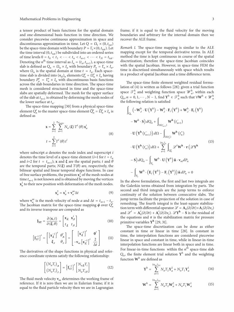
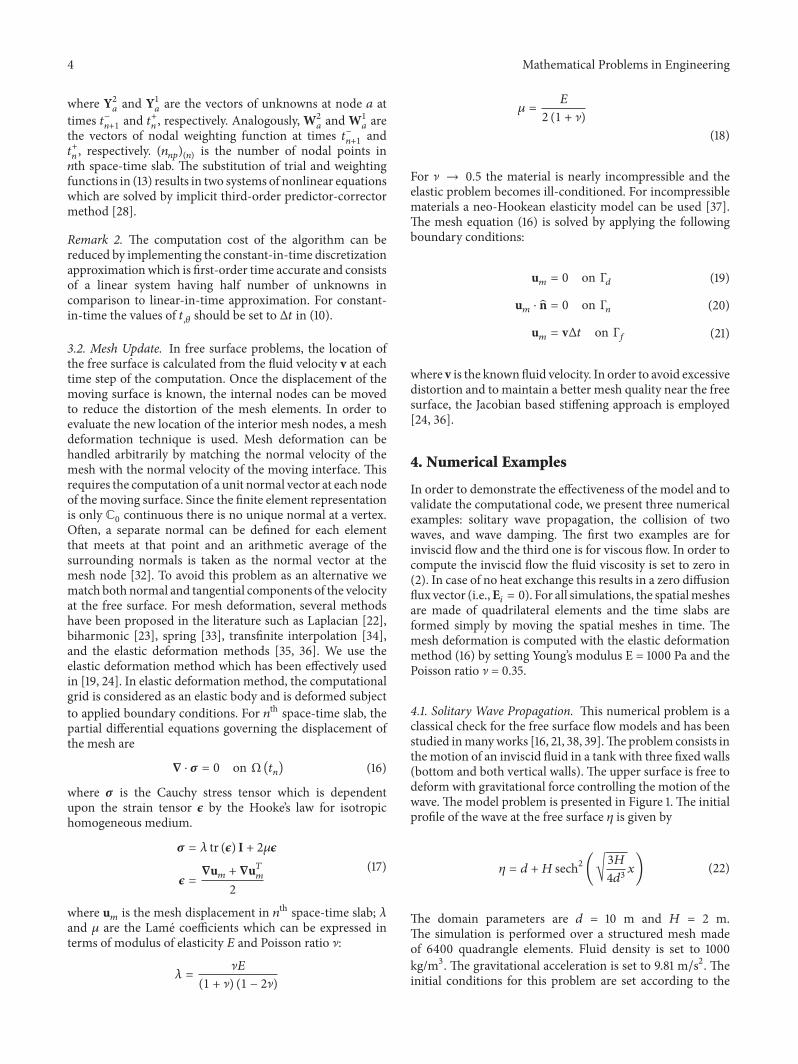
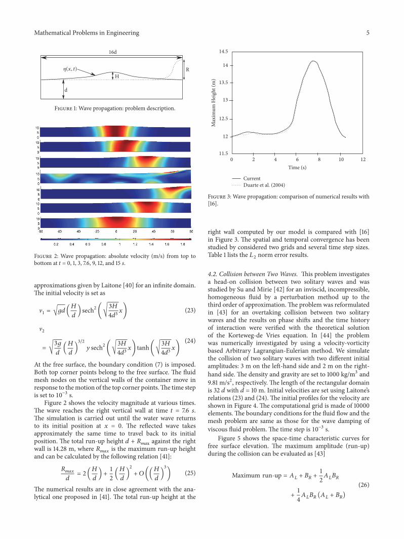
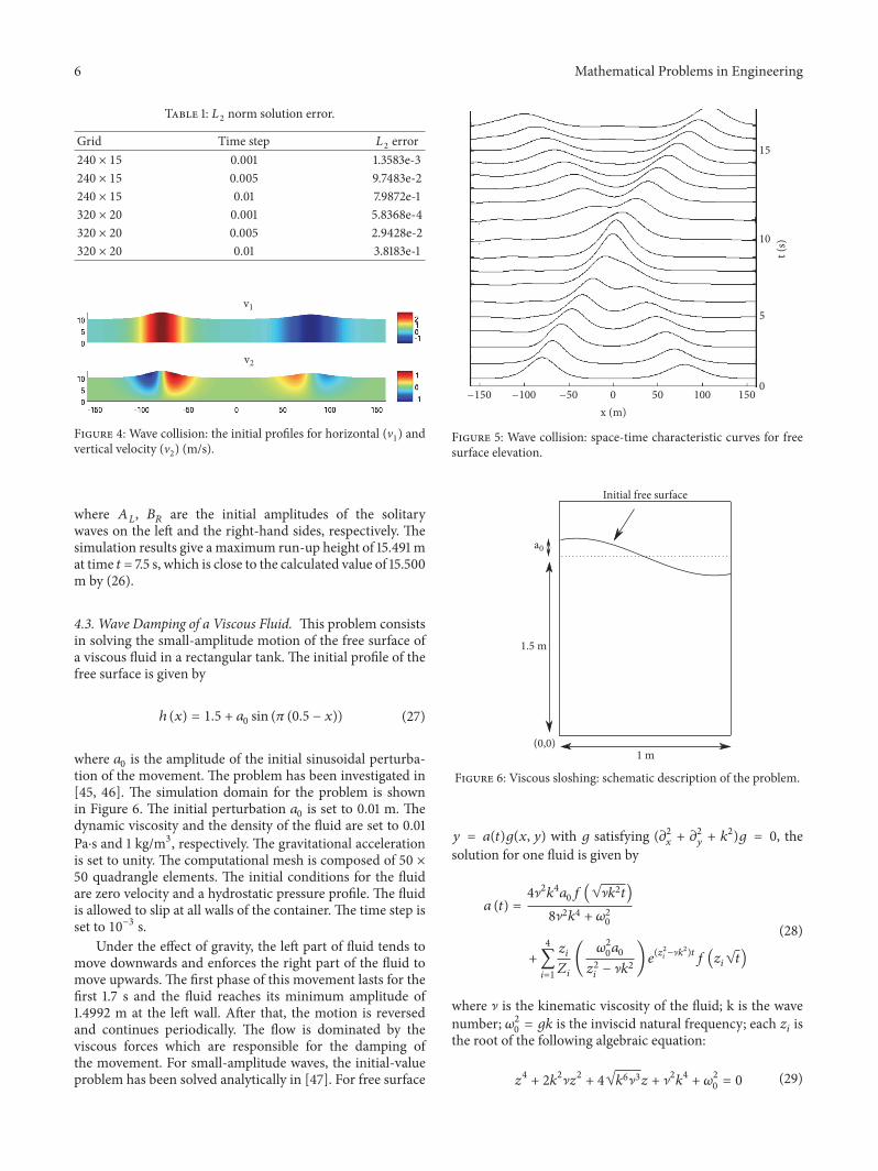
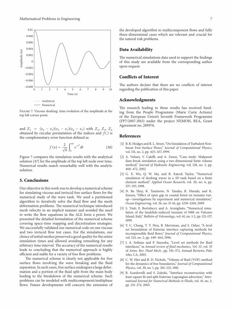
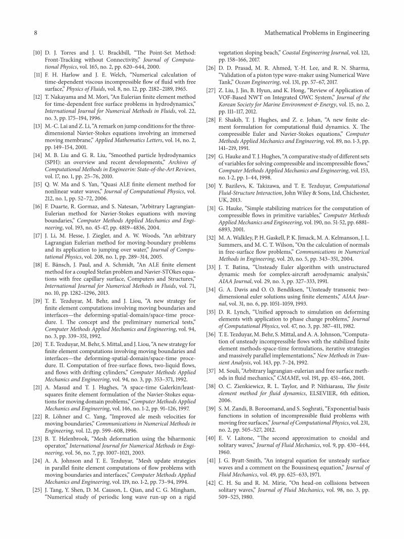
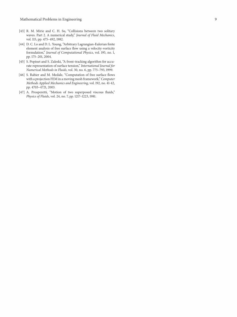

Hindawiwwwhindawicom Volume 2018
MathematicsJournal of
Hindawiwwwhindawicom Volume 2018
Mathematical Problems in Engineering
Applied MathematicsJournal of
Hindawiwwwhindawicom Volume 2018
Probability and StatisticsHindawiwwwhindawicom Volume 2018
Journal of
Hindawiwwwhindawicom Volume 2018
Mathematical PhysicsAdvances in
Complex AnalysisJournal of
Hindawiwwwhindawicom Volume 2018
OptimizationJournal of
Hindawiwwwhindawicom Volume 2018
Hindawiwwwhindawicom Volume 2018
Engineering Mathematics
International Journal of
Hindawiwwwhindawicom Volume 2018
Operations ResearchAdvances in
Journal of
Hindawiwwwhindawicom Volume 2018
Function SpacesAbstract and Applied AnalysisHindawiwwwhindawicom Volume 2018
International Journal of Mathematics and Mathematical Sciences
Hindawiwwwhindawicom Volume 2018
Hindawi Publishing Corporation httpwwwhindawicom Volume 2013Hindawiwwwhindawicom
The Scientific World Journal
Volume 2018
Hindawiwwwhindawicom Volume 2018Volume 2018
Numerical AnalysisNumerical AnalysisNumerical AnalysisNumerical AnalysisNumerical AnalysisNumerical AnalysisNumerical AnalysisNumerical AnalysisNumerical AnalysisNumerical AnalysisNumerical AnalysisNumerical AnalysisAdvances inAdvances in Discrete Dynamics in
Nature and SocietyHindawiwwwhindawicom Volume 2018
Hindawiwwwhindawicom
Dierential EquationsInternational Journal of
Volume 2018
Hindawiwwwhindawicom Volume 2018
Decision SciencesAdvances in
Hindawiwwwhindawicom Volume 2018
AnalysisInternational Journal of
Hindawiwwwhindawicom Volume 2018
Stochastic AnalysisInternational Journal of
Submit your manuscripts atwwwhindawicom