Embed Size (px)
Citation preview
MODELING EFFECTS OF MAIZE PRICE INCREASE ON RURAL
HOUSEHOLD WELFARE: THE CASES OF MTIMAUKANENA IN DOWA AND
MASUMBANKHUNDA IN LILONGWE, MALAWI
Master of Arts (Economics) Thesis
By
STELLA CHIFUNDO NGOLEKA
BSc. (Agricultural Economics)
Thesis Submitted to the Department of Economics, University of Malawi, in partial
fulfillment of the requirements of the degree of Master of Arts in Economics
UNIVERSITY OF MALAWI
CHANCELLOR COLLEGE
June, 2013

DECLARATION
I, the undersigned, declare that this thesis is my original work and that it has not been
submitted for any degree at this or any other University. The opinions expressed in
the study are those of the researcher and do not represent the views of the supervisors
or any organization and therefore errors made herein are mine alone. Where other
researchers’ work has been used, due acknowledgements have been made.
STELLA CHIFUNDO NGOLEKA
________________________________________
Signature
_______________________________________
Date
CERTIFICATE OF APPROVAL
The undersigned certify that this thesis represents the student’s own work and effort
and has been submitted with our approval.
_________________________________
Patrick Kambewa, PhD (Associate Professor of Economics)
First Supervisor
Date: _____________________________
_________________________________
Regson Chaweza, PhD (Lecturer)
Second Supervisor
Date: ____________________________
DEDICATION
I dedicate this work to my daughter Jameela, my late dad Gilbert and mom Elizabeth
who have inspired me to come this far by giving me confidence and a reason to excel.
Dad and Mom, may your souls rest in peace.

v
ACKNOWLEDGEMENTS
I wish to start by thanking God almighty because I would not have made it this
far without His grace, blessings and guidance. I would like to express my sincere
gratitude to my supervisors Associate Professor Patrick Kambewa and Dr. Regson
Chaweza for the continuous support of my MA study and research, for their patience,
motivation, enthusiasm immense knowledge and guidance.
Besides my supervisors, I would like to thank Dr. Evious Zgovu, Dr. Richard
Mussa, Associate Professor Blessings Chinsinga, Mr. Gowokani Chirwa and Mr.
Alick Mphonda for their insightful comments and hard questions.
My gratitude goes to the Evidence for Development and Self Help
Africa for the financial support and the field work. I especially thank Dr. Celia Petty,
Dr. John Seaman and Wolf Ellis whose comments helped to shape this work. I would
also like to thank the team of research assistants that did an amazing job in data
collection.
Many thanks also go to my classmates at Chancellor College and the AERC
Joint Faculty for Electives in Kenya, my friends, the lecturers and the rest of the staff
at the Department of Economics for their support during the entire study period.
In a special way I would like to thank my family for all kinds of support,
motivation and encouragement. Dr. E. Zgovu your confidence in me has really carried
me through. Last but not least my appreciation goes to my dear daughter Jameela Issat
and dear Bashir Issat, my sisters Lydia and Ester Ngoleka for their love and care.

iv
ABSTRACT
This study models the distributional effect of maize price increase on
household welfare in Malawi using the case studies of Mtimaukanena and
Masumbankhunda villages of rural Dowa and Lilongwe districts, respectively. It uses
primary data and employs the Individual Household Method software to analyse the
effect of commodity price increases on households’ disposable income per adult
equivalent. Income is taken as an indicator of poverty or welfare. Results are mixed,
low and middle income households experience income losses as a result of rising
maize prices while large income households who tend to be net maize-sellers show a
significant benefit from higher maize prices.
The stress for poorest households amongst ‘low income’ groups is most severe
with disposable income dropping sharply by averages of 224 percent and 150 percent
in Mtimaukanena and Masumbankhunda villages, respectively. The few net maize-
sellers, high income households record significant gains in income as a result of maize
price increase to such an extent that the overall village-level disposable income rise
with maize prices (4.32 percent and 4.7 percent in Mtimaukanena and
Masumbankhunda villages, respectively). The results suggest the need for policy
interventions including the need to provide safety nets to net-maize buying
households who lose out from rising commodity prices, and intensifying efforts and
programmes aimed at raising maize productivity to ensure low vulnerability to price
changes.

v
TABLE OF CONTENTS
ABSTRACT .............................................................................................................................. iv
TABLE OF CONTENTS ........................................................................................................... v
LIST OF FIGURES .................................................................................................................. ix
LIST OF TABLES .................................................................................................................... xi
LIST OF APPENDICES .......................................................................................................... xii
LIST OF ACRONYMS AND ABBREVIATIONS .............................................................. xiii
CHAPTER ONE ........................................................................................................................ 1
INTRODUCTION ..................................................................................................................... 1
1.0 Background and Motivation ................................................................................................ 1
1.1 Statement of the Problem and Justification of Study ........................................................... 2
1.2 Objectives of the Study ........................................................................................................ 3
1.3 Hypotheses tested................................................................................................................. 3
1.4 Organization of the Study .................................................................................................... 4
CHAPTER TWO ....................................................................................................................... 5
IMPORTANCE OF MAIZE AND OVERVIEW OF AGRICULTURAL SECTOR IN
MALAWI ................................................................................................................................... 5
2.0 Outline.................................................................................................................................. 5
2.1 Overview of Agricultural Sector in Malawi ........................................................................ 5
2.2 Maize Production Regions and Trends in Malawi ............................................................... 6
2.3 Maize Prices Trends in Malawi ........................................................................................... 8
2.4 Maize and Welfare in Malawi ............................................................................................ 10
2.5 The Study Area .................................................................................................................. 11
2.5.1 Mtimaukanena in Dowa district ...................................................................................... 11
vi
2.5.2 Masumbankhunda in Lilongwe....................................................................................... 12
CHAPTER THREE ................................................................................................................. 13
LITERATURE REVIEW ........................................................................................................ 13
3.0 Outline................................................................................................................................ 13
3.1 Theoretical Framework ...................................................................................................... 13
3.1.1 Consumer Choice Theory ............................................................................................... 13
3.1.2 Consumer Surplus Theory .............................................................................................. 18
3.2 Welfare Measurements of Price Changes .......................................................................... 21
3.3. The Food entitlement theory ............................................................................................. 22
3.3.1 Individual Household Method ........................................................................................ 23
3.4 Poverty Analysis ................................................................................................................ 24
3.5 Empirical literature ............................................................................................................ 26
3.6 Conclusion ......................................................................................................................... 28
CHAPTER FOUR .................................................................................................................... 29
METHODOLOGY .................................................................................................................. 29
4.0 Outline................................................................................................................................ 29
4.1 Research Design................................................................................................................. 29
4.1.1 Data Collection Method and Sampling design ............................................................... 30
4.2 Analytical Framework ....................................................................................................... 34
4.2.1 Salient Features of the IHM Model ................................................................................ 34
4.2.2. Limitation of the Study Methodology............................................................................ 36
4.3Model Specification ............................................................................................................ 36
4.4 Data Analysis ..................................................................................................................... 38
4.4.1 Welfare Measures and Poverty Analysis ........................................................................ 39
4.4.2 Price Data ........................................................................................................................ 39
vii
4.5 Presentation of Results ....................................................................................................... 40
4.5.1 Baseline ........................................................................................................................... 40
4.5.2 Simulation ....................................................................................................................... 40
4.6 Description of Key Variables Considered in the Study ..................................................... 41
4.7 Some Methodological Issues ............................................................................................. 44
4.8 Equivalence Scales............................................................................................................. 45
4.9 Counter Factual Analysis ................................................................................................... 45
4.10 Correction for errors ........................................................................................................ 45
CHAPTER FIVE ..................................................................................................................... 46
EMPIRICAL RESULTS AND ANALYSIS ........................................................................... 47
5.0 Outline................................................................................................................................ 47
5.1 Brief of Focus Group Discussion ....................................................................................... 47
5.2 Socio-Economic and Demographic ................................................................................... 48
5.2.1 Descriptive Analysis of the Data .................................................................................... 55
5.2.2 Contribution of Maize Income to Household Income .................................................... 59
5.3 Simulation Results ............................................................................................................. 70
5.3.1 Modelling of Maize Price Increase on Household Disposable Income .......................... 70
5.3.2 Change in Individual Household Poverty due to Maize Price Increase.......................... 79
5.5 Conclusion ......................................................................................................................... 85
CHAPTER SIX ........................................................................................................................ 86
CONCLUSIONS...................................................................................................................... 86
6.1Summary of the Study ........................................................................................................ 86
6.2. Main Findings and Conclusions........................................................................................ 86
6.3 Policy Implications ............................................................................................................ 87
6.4Study Limitations and Area for Further Research .............................................................. 88

viii
REFERENCES ........................................................................................................................ 89
APPENDICES ......................................................................................................................... 98
ix
LIST OF FIGURES
Figure 1.1: Food and Agricultural Organisation (FAO) Annual Price Index ............................ 1
Figure 2.1: Maize Price Trends, May 2010 - December 2012 ................................................... 9
Figure 3.1: Effects of Increases in Commodity Prices of Normal Good ................................. 14
Figure 3.2: Effects of Increases in Commodity Prices of Giffen good .................................... 17
Figure 3.3: Changes in Consumers' and Producers' Surplus .................................................... 19
Figure 5.1: Population pyramid ............................................................................................... 51
Figure 5.2: Contribution of Maize to Household Cash Income by income quintile,
Malawi Kwacha, Mtimaukanena ........................................................................... 60
Figure 5.3: Contribution of Maize to Household Income in Cash by income quintile,
Malawi Kwacha, Masumbankhunda ...................................................................... 61
Figure 5.4: Contribution of Maize Food Income to Total Food Income Consumed
(Total Energy in Kilocalorie), Mtimaukanena ....................................................... 63
Figure 5.5: Contribution of Maize Food Income to Total Food Income Consumed (%
of Total Food Energy), Masumbankhunda ............................................................ 64
Figure 5.6: Household Disposable Income before and after an 80% Maize Price
Increase in Mtimaukanena ..................................................................................... 71
Figure 5.7: Household Disposable Income before and after An 80% Maize Price
Increase in Masumbankhunda ................................................................................ 72
Figure 5.8: Household Disposable Income before and after an 95% maize price
Increase in Mtimaukanena ..................................................................................... 75
Figure 5.9: Household Disposable Income before and after a 95% maize price
Increase in Masumbankhunda ................................................................................ 76
x
Figure 5.10: Standard of Living Threshold and 80% Maize Price Increase Simulation
for the Poor Households in Mtimaukanena ........................................................... 81
Figure 5.11: Standard of Living Threshold and 80% Maize Price Increase Simulation
for the Poor Households in Masumbankhunda ...................................................... 83

xi
LIST OF TABLES
Table 2.1: Maize Production, Consumption and Maize Deficit Situation in Malawi
2007– 2013............................................................................................................... 7
Table 5.1: Age and Sex distribution ........................................................................................ 49
Table 5.2: Median age by income quintile and population of the village ................................ 52
Table 5.3: Dependency ratio per quintile of Disposable Income per Adult Equivalent .......... 52
Table 5.4: Demographic characteristics of households by income quintile ............................ 53
Table 5.5: Descriptive Statistics of Income by Source in Malawi Kwacha and Kcal,
Mtimaukanena........................................................................................................ 56
Table 5.6: Contribution of Maize to Total Cash Income by Income quintile, Malawi
Kwacha .................................................................................................................. 62
Table 5.7: Household Budget for Selected Maize Food Surplus and Deficit Producer .......... 67
Table 5.8: Relationship between Maize Net Buying/Selling and Income Status ................... 69
Table 5.9: Simulated Changes in Disposable Income, Mtimaukanena ................................... 77
Table 5.10: Simulated Changes in Disposable Income, Masumbankhunda ............................ 78

xii
LIST OF APPENDICES
Appendix 1: Average Monthly Maize Price in Malawi Kwacha per Kilogram ...................... 98
Appendix 2a: Items used in establishing STOL, Masumbankhunda ....................................... 99
Appendix 2b: IHM Interview Form ....................................................................................... 100
Appendix 3: Map of Malawi showing Livelihood Zones and their activities ....................... 112
xiii
LIST OF ACRONYMS AND ABBREVIATIONS
ADMARC Agricultural Development and Marketing Corporation
CV Compensating Variation
DI Disposable Income
EV Equivalent Variation
FAO Food and Agricultural Organization
FEWS_NET Famine Early Warning Systems Network
GDP Gross Domestic Product
GNI Gross National Income
HEA Household Economy Approach
IHM Individual Household Method
IHS Integrated Household Survey
LDC Less Developed Countries
MDGs Millennium Development Goals
MGDS Malawi Growth and Development Strategy
MoAFS Ministry of Agriculture and food Security
MK Malawi Kwacha
MVAC Malawi Vulnerability Assessment Committee
NBR Net Benefit Ratio
NSO National Statistics Office
SOLT Standard of Living Threshold
TA Traditional Authority
UN United Nations

xiv
US$ United States Dollar
VAC Vulnerability Assessment Committee
WB Word Bank
1
CHAPTER ONE
INTRODUCTION
1.0 Background and Motivation
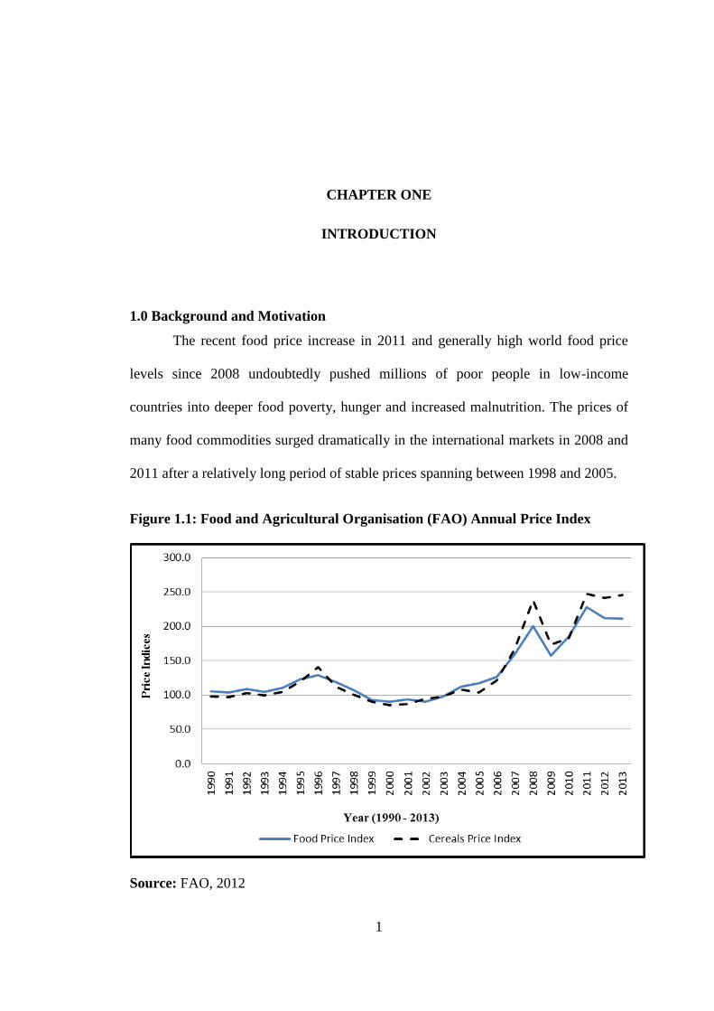
The recent food price increase in 2011 and generally high world food price
levels since 2008 undoubtedly pushed millions of poor people in low-income
countries into deeper food poverty, hunger and increased malnutrition. The prices of
many food commodities surged dramatically in the international markets in 2008 and
2011 after a relatively long period of stable prices spanning between 1998 and 2005.
Figure 1.1: Food and Agricultural Organisation (FAO) Annual Price Index
Source: FAO, 2012

1
Figure 1.1 shows that international food prices spiked in 2011. The food price
index increased by 24 percent, and the cereal price index increased by 43 percent
between 2011 and 2012 periods.1 At the peak in the middle of 2011, international
prices of wheat and maize went up by 74 percent (World Bank, 2011). The FAO
(2012) warns of the need for an urgent assessment of the effects of increased food
prices on poor and non-poor households in Less Developed Countries (LDC), given
the recent food price peak.
Most poor households in developing countries live in rural areas and are staple
food producers, consumers, buyers and sellers. This study focuses on Malawi, one of
the poor developing countries with a GDP of only US$ 5.621 billion in 2011 with an
estimated population size of 15.38 million people (World Bank, 2011). In Malawi,
maize is the staple food. Staple food prices in Malawi increased steadily in 2011 and
even more sharply in 2012. More specifically, the price of maize at formal markets
rose from 30 Malawi Kwacha (MK), the February 2010 price to MK 52 per kilogram
in March 2011 then further up to MK 60 per kilogram in November 2011. Such hefty
and sustained price increases undoubtedly bore some adverse effects on a number of
parameters including on household real income, food security and nutrition amongst
both urban and rural households given the initial conditions of widespread poverty
and food insecurity in Malawi. This study sought to carry out a systematic
investigation into these questions to understand the scale and scope of the impacts
with a view to inform appropriate policy analysis and direction.
1 Food price index consists of all food commodities. Cereals price index is compiled using the grains
and rice price indices. The Food Price Index weighs export prices of a variety of food commodities
around the world in nominal U.S. dollar prices, taking 2005 as the reference year

2
1.1 Statement of the Problem and Justification of Study
Despite consecutive years of surplus maize harvest in Malawi from 2007 to
date, Malawi has experienced continuous price escalation of maize commodities over
time. The real price of maize in Malawi has increased by 141 percent between 1998
and 2008 and according to (FEWS_NET, 2012) maize price increased by 80 percent
between 2011 and 2012. The increase in staple food prices raise concerns about
welfare effects that this can have, particularly among poor household and those with
incomes just above the poverty line (Hoyos and Medvedev, 2008).
According to the Integrated Household Survey (IHS-2) data, the average
household per capita expenditure (including the opportunity value for all own-
produced foods) amounts to US$ 0.54 per day, of which 73 percent is spent on food.
Own-produced food adds up to 58 percent of the total food quantity consumed and the
opportunity value corresponds to half of the total food expenditure (NSO, 2005).
Doward et al., (2010) estimated that 60 percent of households in Malawi are regular
maize buyers and, as such, are vulnerable to maize price fluctuations. In Malawi many
rural households have adequate maize stocks soon after harvest. Most poor
households on average have maize stocks from own production which tend to last
four months after harvest.
While there are only a limited number of studies that estimate the numbers of
net food buyers and sellers and their incomes, there has been a consensus that high
food prices are bad for the poor because most of the poor are net food buyers, even in
rural areas (Seshan and Umali-Deininger, 2007; Byerlee et al., 2006; Ivanic and
Martin, 2008; Aksoy and Isik-Dikmelik, 2008; Dessus et al., 2008; and Rios et al.,
2008). The poor are also likely to be more significantly affected by price changes:

3
Engel’s law states that poor people spend a greater proportion of their income on food
(Varian, 2005).
The effects of recent maize price increases on rural welfare in Malawi are not
yet established. This study explores these effects, simulating the potential impact of
high maize prices on rural households’ income and welfare in selected maize-
producing areas of the Kasungu-Lilongwe plain and providing important insights for
policy makers.
1.2 Objectives of the Study
The general objective of the study is to model the distributional effect of maize
price increase on income and welfare of the rural households in Malawi. In order to
achieve this, the following specific research objectives were formulated;
i. To model the effect of maize price increase on household disposable income
ii. To examine the change in household poverty due to maize price increase
iii. To assess the contribution of maize income to household income
1.3 Hypotheses tested
Based on the objectives of the study, the paper examined the following null
hypotheses:
i. Maize price increase does not have effect on household disposable income;
ii. Maize price increase does not have effect on individual household poverty;
and,
iii. Maize income does not contribute to household income
4
1.4 Organization of the Study
The rest of the study is organized in five chapters; Chapter Two gives an
overview of agricultural sector and importance of maize in Malawi. Chapter Three
reviews the relevant literature whereby food price and welfare is discussed from a
theoretical perspective and the major empirical studies on staple food price increase as
well as welfare relevant to this study are discussed. Chapter Four describes the
methodology in which Individual Household Method (IHM) modeling of price change
is simulated as specified by Evidence for Development. Chapter Five presents and
discusses the empirical results. It gives the interpretation of the results obtained from
the analysis both on baseline and simulations. Finally, Chapter Six provides the policy
implications of the results obtained, as well as the concluding remarks, and the
limitation of the study.

5
CHAPTER TWO
IMPORTANCE OF MAIZE AND OVERVIEW OF AGRICULTURAL
SECTOR IN MALAWI
2.0 Outline
This chapter presents an overview of agricultural sector and importance of
maize in Malawi. Thereafter it describes production and maize price trends. The final
section of this chapter describes the study area.
2.1 Overview of Agricultural Sector in Malawi
The agricultural sector in Malawi is the mainstay of the Malawian economy.
The sector contributes about 34 percent of GDP, 81 percent of employment and 90
percent of exports. It supplies more than 65 percent of the manufacturing sector’s raw
materials, provides 64 percent of the total income of the rural people (Word Bank,
2009). Main export commodities are tobacco, tea and sugar. The sector consists of
subsistence farming which result to poor agricultural commodity estimates, low
quality and high volatility of agricultural commodity prices within a year. Agriculture
is the main livelihood of the majority of rural people, who account for more than 85
percent of the estimated 14 million people in 2005. Eleven percent of the rural labour

6
force works on agricultural estates to supplement farm income, and around 80 percent
is engaged in the smallholder sub-sector (Word Bank, 2008). Smallholder agriculture
is mainly rain fed and done by human labour with hand-held hoes.
Maize, the main staple food occupies 60 percent of cultivated land. According
to Grant et al., (2012) consumption of maize is divided into four main categories:
direct human consumption, animal feed consumption, maize processed for industrial
uses and bio-fuels. The level of maize in industrial use in Malawi is small or
negligible. Some processed maize products are mainly exported to other countries.
Chibuku beer is the main industrial product produced from maize.
2.2 Maize Production Regions and Trends in Malawi
According to Malawi Vulnerability Assessment Committee (MVAC, 2012),
the country enjoys a variety of ecological zones broadly grouped into: lower Shire
valley, lakeshore and low-lying rain shadow areas, medium altitude areas, and high
attitude plateau and hilly areas. Maize is grown in virtually all four agro-ecological
zones of Malawi but mainly in medium altitude areas covering part of the central
region of Malawi exclusively Kasungu-Lilongwe plain (see appendix 3). Maize
production in Malawi is limited by high costs and sub-optimal use of chemical
fertilizers under continuous cultivation. Malawi has been designing programs to
increase maize production. For instance, to ensure food security Malawi introduced
subsidy program and this has resulted into higher production in good weather
conditions and reduction in the import of maize. Below is the table showing Maize
production, consumption and Maize deficit situation in Malawi from 2007 to 2013.

7
Table 2.1: Maize Production, Consumption and Maize Deficit Situation in
Malawi 2007– 2013
Consumption
year
Maize
production
(million MT)a
Maize surplus
(Million MT)
Number of
People
affected
Maize
Equivalent
Required (MT)
Cash Equivalent
Required
(MK’000)
2007/08 3.2 1.2 63,234 610 81,000
2008/09 2.9 0.5 613,291 16,806 942,000
2009/10 3.6 1.2 275,168 10,984 573,000
2010/11 3.2 0.53 508,089 28,602 1,138,000
2011/12 3.9 1.2 272,500 6,756 405,000
2012/13 3.6 0.8 1,630,007 75,394 6,031,500
Source: MVAC 2013
a Metric tonnes (MT)
Table 2.1 shows production trends between 2007/2008 to 2012/2013 period.
Maize production level increased in 2011/2012 with a surplus of 1.2 million metric
tonnes. Furthermore, the table shows a national increase in production in 2011/2012
compare to the past four years. There was a need of distribution of 6,756 maize
equivalent metric tonnes to affected people in 2011/2012 which is equivalent to MK
405,000, 000. This shows that the national food security situation do not indicate
sufficient maize at household, most households in Malawi do not produce adequate
food to last them throughout the year. Hence, investigating welfare changes at
household level is particularly important because even when countries improve
national food self-sufficiency, due to production surplus and entitlement gains,
national economic growth and food self-sufficiency hardly translates into household
welfare improvements.
8
Despite maize surplus in 2011/2012 agricultural year, MVAC reported food
vulnerability among a significant number of households as indicated in the figure.
This resulted to maize exporting ban policy which was implemented in December
2011. Malawi banned export of maize, this policy was implemented when it became
long dry period threatened to cause a maize shortage and following the report from
MVAC. However, the ban did not prevent traders from smuggling maize across the
border into neighboring countries like Tanzania, Zambia and Mozambique and storing
tons of maize in their local warehouses and houses which led to further low supply
and scarcity of maize at the market.
2.3 Maize Prices Trends in Malawi
During the last quarter of 2011, maize prices increased rapidly. In central
region local markets maize was sold at an average of 70 Malawi Kwacha per kilogram
in January, 52 percent above November’s prices. Since the end of 2011, monthly
prices of maize rose rapidly aggravating food insecurity conditions in Malawi
(MVAC, 2012). According to FEWS_NET (2012) maize prices rose in 2011/2012
due to two major factors which are: (1) adjustment to maize prices by the
government-owned food commodity trader ADMARC from MK 30 to MK 52 per
kilogram then MK 60 per kilogram due to low supply of maize in the market because
of bad weather experienced in the 2010/2011 production season, and (2) the scarcity
of fuel in petrol pumps that was brought on by limited foreign currency in the country.
Figure below shows monthly average price of maize in Malawi.

9
Figure 2.1: Maize Price Trends, May 2010 - December 2012
Source: Ministry of Agriculture and Food Security (MoAFS, 2013)
Figure 2.1 shows average prices collected by MoAFS monthly in local
markets. Actual figures are shown in appendix 2a. As indicated in the figure, in
2010/2011 the average monthly prices of maize were around MK 30 per kilogram. In
2011/2012 agricultural year the average price was MK 36.89 per kilogram. The
highest average monthly price was registered in January of about MK 56.23. The
lowest average monthly price was registered in May of about MK 23.75. This implies
that there was a wide range in maize prices at local markets considering that the
average monthly prices are weighted from average daily prices then average weekly
prices.

10
The maize prices in Malawi are highly affected by seasonality as shown from
the figure. Chirwa (2004) reported that Malawi has high volatility of maize price
compare with many countries in Southern Africa Developing Countries (SADC)
region. The subsistence farming as opposed to commercial farming is one of the
reasons for this volatility. The MoAFS calculated an average price increase of 80
percent at both formal and local markets. The 80 percent increase was found using the
weighted average which consider months and number of buyers and sellers at the
markets.
2.4 Maize and Welfare in Malawi
In Malawi, food security has been historically defined in terms of national
self-sufficiency in maize (World Bank, 2003). Most government reports place maize
at the centre of food security and agricultural development policy. The food policy
emphasis prior to the 1990s was centred on achieving self-sufficiency in food or
maize production. As a result most agricultural research and extension services
concentrated on improving productivity in maize production (Msukwa, 1994). The
Malawi Growth and Development Strategy (MGDS) also aims at putting in place
measures to protect those who temporarily fall into poverty through measures to
increase assets for the poor to ensure improved access to staple food, maize.
Building on the Vision 2020, the MGDS is centered on achieving strong and
sustainable economic growth, building a healthy and educated human resource base,
and protecting and empowering the vulnerable. It seeks to ensure economic growth,
economic empowerment and food security through ensuring availability of timely and
quality food to all citizens so that Malawians are less vulnerable to shocks.
11
2.5 The Study Area
The study was conducted in Central Region of Malawi involving Dowa and
Lilongwe. In terms of livelihood zone the two districts are in Kasungu-Lilongwe
plain. Kasungu-Lilongwe plain comprises six districts namely Kasungu, Dowa,
Lilongwe, Mchinji Ntchisi, Dedza and partially Mzimba South. Kasungu-Lilongwe
plain was selected for this study because it registered low volatility to maize prices in
2011/2012 agricultural year due to its high maize production and surplus compare to
other plains in Malawi.
Dowa and Lilongwe districts are in the medium attitude zone. The zone enjoys
high average rainfall ranging from 800 – 1,200 mm annually with an attitude of 1,000
to 1,500 metres above sea level. Kasungu-Lilongwe Plain is Malawi’s breadbasket.
The farming population is estimated at around 1.5 million households. In an average
year, the zone produces surplus food crops such as maize, groundnuts, sweet potatoes
and Soya bean (MVAC, 2012). The villages selected for the study were
Mtimaukanena and Masumbankhunda in Dowa and Lilongwe districts respectively.
2.5.1 Mtimaukanena in Dowa district
The main tribe in Dowa is Chewa, however, there are some Yaos in the
district. Main crops grown in the district are tobacco, maize, cotton, groundnuts and
sweet potatoes. Mtimaukanena village in Traditional Authority (TA) Mtukula in
Dowa district was sampled for this study. This village is in Chabvala Extension
Planning Area (EPA) of Dowa District Agricultural Development Office under the
Kasungu Agricultural Development Division (KADD).
The village, lies on the southern end of Dowa district marking a boundary with
Lilongwe district with Lilongwe City some 40 km away. The area is situated next to
Kamuzu International Airport and Lumbadzi trading centre both of which are

12
important economic entities for the study area. The major food crop is maize with
tobacco and ground nuts as major cash crops. The village has fertile soil with dimba2
for winter maize and vegetable cultivation.
2.5.2 Masumbankhunda in Lilongwe
In Lilongwe district, Chewa is the major tribe accounts for 99 percent of the
total population in the rural area of the district. Lilongwe grows both cash and foods
crops and are grown through smallholder farming and estate farming. Maize of both
high and low yielding dominates the smallholder farming system. The study was
specifically conducted in Traditional Authority Masumbankhunda in Kumulandi and
a Poondo village in Malingunde Extension Planning Area (EPA) of Lilongwe District
Agricultural Development Office under the Lilongwe Agricultural Development
Division (LADD). Additional to maize the major cash crop in the village are ground
nuts, paprika and tobacco.
2 Low land
13
CHAPTER THREE
LITERATURE REVIEW
3.0 Outline
This chapter reviews both theoretical and empirical literature that explores the
impact of food price increase at both macro and micro level. Theoretical literature
provides a household modeling framework and an understanding of price change an
external shock which can affect household welfare. The empirical literature provides
findings based on appropriate modeling framework and theory around the area of
interest.
3.1 Theoretical Framework
3.1.1 Consumer Choice Theory
Since a staple food price change is a market phenomenon which can have
effects to a rational consumer, it is explained using consumer theory and consumer
surplus theory. Consumer theory examines how consumers make choices under
income or budget constraints. For rational consumer if price increases there will be
two effects. These effects are income effects and substation effects. According to
Varian (2005) and Mas-Collel (1995), at higher prices, the quantity demanded is less
than at lower prices.
14
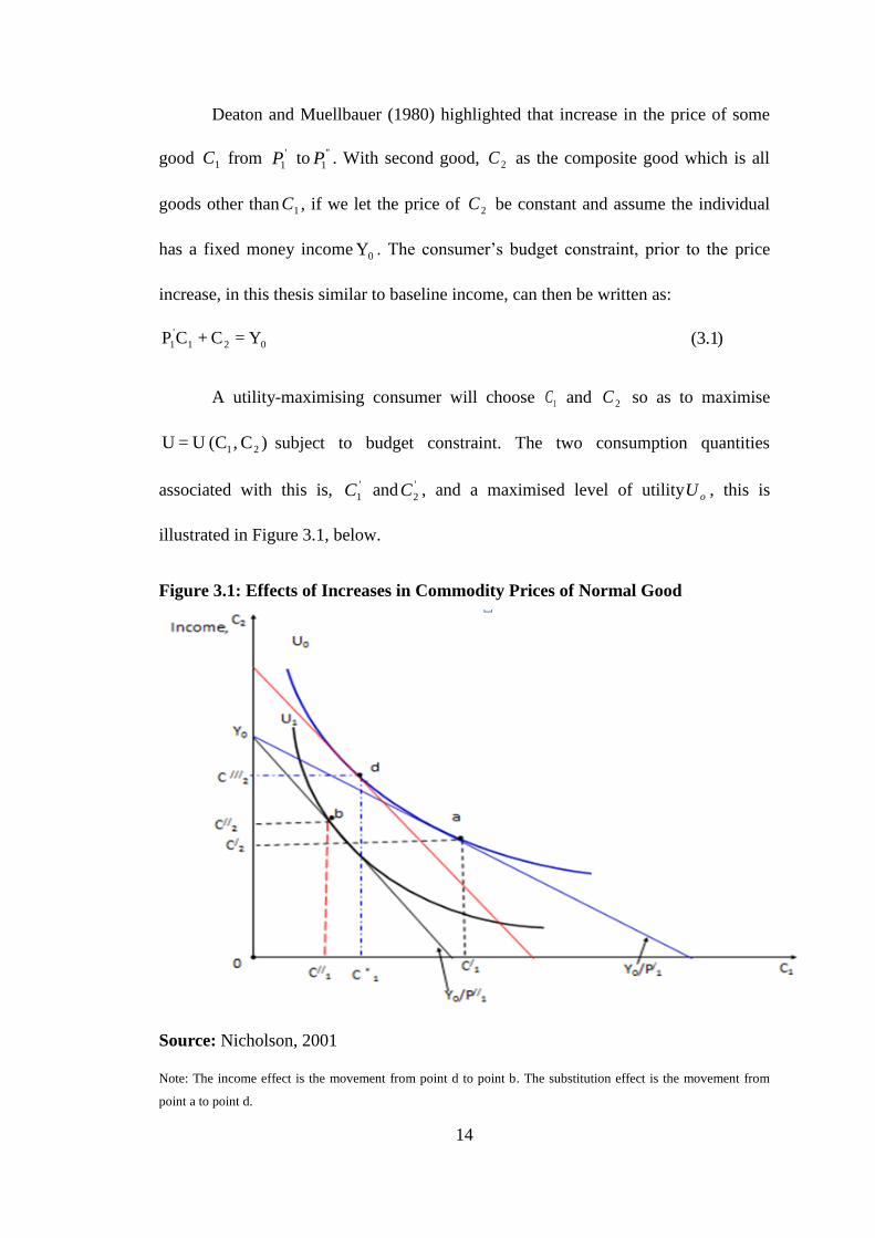
Deaton and Muellbauer (1980) highlighted that increase in the price of some
good 1C from '
1P to ''
1P . With second good, 2C as the composite good which is all
goods other than 1C , if we let the price of 2C be constant and assume the individual
has a fixed money income0Y . The consumer’s budget constraint, prior to the price
increase, in this thesis similar to baseline income, can then be written as:
Y = C+ CP 021
'
1 )1.3(
A utility-maximising consumer will choose 1C and 2C so as to maximise
)C ,(C U= U 21 subject to budget constraint. The two consumption quantities
associated with this is, '
1C and '
2C , and a maximised level of utility oU , this is
illustrated in Figure 3.1, below.
Figure 3.1: Effects of Increases in Commodity Prices of Normal Good
Source: Nicholson, 2001
Note: The income effect is the movement from point d to point b. The substitution effect is the movement from
point a to point d.

15
In Figure 3.1 in a case of the price increase of good1C (assuming maize in this
thesis) from '
1P to ''
1P (the change from higher price to lower price) the budget
constraint will rotate clockwise about the point 0Y on the vertical axis to the new
constraint
021
' Y = C + CP )2.3(
As shown in the figure, Utility maximisation now will imply consumption
levels of ''
1C and ''
2C at point b and a lower utility level 1U . The decrease in the
consumption of 1C (maize) from '
1C to ''
1C can be decomposed into a substitution
effect and '
1C to *
1C , is an income effect.
Figure 3.1 show that, a change in the price of commodity 1C alters the slope
of the budget constraint. Even if the individual remained on the same indifference
curve 0U , as shown in the figure his optimal choice will change from a to d . Hence
this will give the substitution effect. In this context, the theory can be applied to maize
price change in the following way. All things being equal, a maize net buyer
household or household with deficit in maize own production will depend on
purchasing maize at the market. This household in a short run will face a substitution
effect as the price of maize rises because maize becomes relatively more expensive.
The substitution effect is observed when assuming other alternative food like
cassava and sweet potato presented as 2C in Figure 3.1 stay at the same price, they
become relatively cheaper.
The consumers will switch from maize initially consumed at optimal choice
‘a’ and buy relatively cheaper one in order to maximize utility. Hence consuming at
optimal point ''d of same indifference curve )( 0U but with more of other goods
16
)( 2C compare to maize consumed at optimal choice ‘a’. This depends on the utility
derived from consuming that other commodity and its price, subject to the
individual’s income. However this shift can affect the household food kilocalorie in
take because maize is a staple food for Malawi and relatively provide high energy per
kilogram compare to alternative staple foods. Objective Three of this thesis analyses
the contribution of maize to household both in kilocalorie and cash income.
The price change alters the individual’s “real” income buy making maize
commodity relatively expensive with income remaining constant. Therefore the
individual move to a new indifference curve illustrated in the figure, this is the
movement from 0U to 1U and gives the income effect as shown. At point ‘b’ and
individual is at a lower indifference curve implying maize price increase has reduced
the consumers utility. At that point the individual is consuming less of other goods as
well. These include both food and non-food cost like school fees, soap, paraffin and
clothes which implies effect on individual welfare.
On the other hand, in a case of a staple food in developing countries like
Malawi mostly a staple food is considered Giffen goods. Giffen goods are those
which are consumed in greater quantities even when their price rises. Giffen good is a
staple food, such as rice or maize which forms large percentage of the diet of the
poorest sections of a society, and for which there are no close substitutes (Varian,
1992 and Gravelle and Rees, 2004). A rise in the price of such a staple food will not
result in a typical substitution effect to food commodity; instead it can have an effect
to their welfare by reducing the consumption of their non-food items. In a case of a
fall in real incomes of the poor they would tend to buy more of the staple good from
their income as figure 3.2 illustrates.

17
Figure 3.2: Effects of Increases in Commodity Prices of Giffen good
Source: Varian, 2005
Figure 3.2 shows that an increase in price of maize results in a reduction in
consumption of other goods when prices of other goods remain constant. This will
have an effect on welfare in that; if a consumer was consuming combination of maize
and other goods at optimal choice a , when the price of maize increases in a case of
maize being a Giffen good the consumer will reduce consumption of other goods.
This is necessitated by the fact that an increase in price of maize leads to reduction in
real income because there are no close substitutes to staple food. In this case the
consumer will prioritise diet resulting to purchasing more maize to avoid being
affected by maize price inflation and use the remaining money to buy other
commodities.

18
In case of constant budget consumers will reduce consumption of other goods
such as basic needs like paraffin, clothes, school fees and health care. This indicates
that an increase in staple food is bad and will lead to loss of welfare to rational
consumers. A welfare loss is observed in that even though money income remains
constant, changes in price of maize will change purchasing power, and thereby
changes demand.
However, one can still criticise the theory in as far as welfare is concerned in
that it does not fully explain the effect on welfare. This is so since it only explains the
effects to quantity demanded to price increase on consumer without necessary
gauging the welfare effects to the dual household. Due to dual nature of rural
households in Malawi of being both a producer and a consumer of maize this theory
alone will not provide theoretical of a price change. The thesis therefore, also used the
consumer surplus theory.
3.1.2 Consumer Surplus Theory
In Malawi rural households are both consumers and producers of maize. Due
to dual nature of rural households, consumer surplus theory can illustrate the price
change and its relationship to welfare. In this theory, it is assumed that individuals are
rational and have both quasilinear and no quasilinear utility. In the case of no
quasilinear utility, the price at which a consumer is willing to purchase some amount
of good like maize will depend on how much money he has for consuming other
goods which include both food and non food goods. The price policy effect can be
reflected in the changes in welfare of individuals. Market policy can affect
individuals’ welfare through changes in the consumer or producer surplus as
illustrated in figure 3.3 below.
19
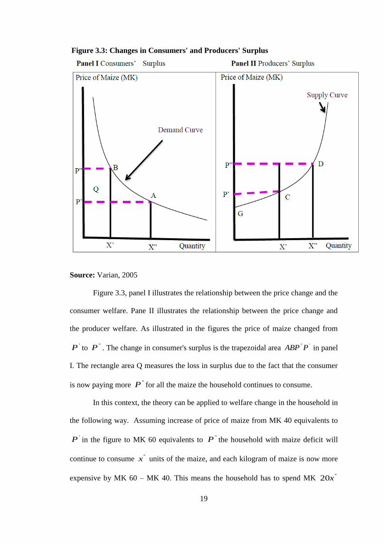
Figure 3.3: Changes in Consumers' and Producers' Surplus
Source: Varian, 2005
Figure 3.3, panel I illustrates the relationship between the price change and the
consumer welfare. Pane II illustrates the relationship between the price change and
the producer welfare. As illustrated in the figures the price of maize changed from
'P to ''P . The change in consumer's surplus is the trapezoidal area
''' PABP in panel
I. The rectangle area Q measures the loss in surplus due to the fact that the consumer
is now paying more ''P for all the maize the household continues to consume.
In this context, the theory can be applied to welfare change in the household in
the following way. Assuming increase of price of maize from MK 40 equivalents to
'P in the figure to MK 60 equivalents to ''P the household with maize deficit will
continue to consume ''x units of the maize, and each kilogram of maize is now more
expensive by MK 60 – MK 40. This means the household has to spend MK ''20x
20
more money than the household did before the price change just to consume ''x units
of maize. However this alone does not give the entire welfare loss. The welfare loss is
observed when the net buyer household has decided to consume less of maize )( ''x
than it was consuming before )( 'x the price change. Hence two effects observed here
are the loss from having to pay more for the units the household continues to consume
and loss from the reduced consumption. Consumer's surplus, an area under the
demand curve will give the short run welfare loss.
On the other hand a household which is a net seller of maize will have a
producer surplus by selling maize at a higher price (60 Malawi Kwacha) than the
actual price (40 Malawi Kwacha) the producer was willing to sell before the price
change. The area of CGP '' in panel II gives the change in maize producer's surplus
due to the increase in the price of maize. Area ''' PCDP is equivalent to profit that the
maize selling household will gain to maize price increase. It is worth note that in rural
area where households are both maize sellers and maize buyers the effect will depend
on the difference between the two, whether the household is a net buyer or net seller.
From these two theories, among others, Slutsky effect model, compensating variation
and net benefit ratio as measures of welfare emerged.
21
3.2 Welfare Measurements of Price Changes
Varian (2005) highlighted that Slutsky identity implies the total change in
demand equals the substitution effect plus the income effect. Varian showed that the
substitution effect is always negative but the total income effect can be positive or
negative. The households with deficit maize are adversely affected by a higher food
price pushing the budget constraint outward giving the negative Slutsky effects on
food demand. On the other hand, producer household assuming food is a normal good
the total income effect is positive due to profit effect. If this profit effect outweighs
the Slutsky effects, there will be welfare gain to producer households.
The consumer model and Slutsky effects illustrates that, a negative “real
income” effect reinforces a negative “substitution” effect; this is illustrated in Figure
3.1. This concept is applied in this study in that, the study area is a maize producing
area with surplus of maize in good weather periods. This can imply a gain in welfare
from maize price increase in the study area if there was maize surplus in the reference
year. However, substitution effect can be observed in a longitudinal data. The study
used cross sectional data.
Nicholson (2001) highlighted that the impact of price changes on household
welfare is often calculated using Consumer Surplus or the Equivalent Variation or the
Compensating Variation. The modified concept of compensating variation was
developed by Deaton and Muellebauer (1980) and Minot and Goletti (2000). This
evaluation of welfare and distributional impacts of price changes looks at measures of
Compensating Variation. Compensating Variation is the amount of money sufficient
to compensate households following price changes and enable them to return to the

22
initial levels of utility (Benfica, 2012). The concept of compensating variation as a
welfare analysis has been widely used in empirical literature.
Deaton (1989) and Ravallion (1998) developed net benefit ratio (NBR) as a
welfare measure. The method is used to estimate a short run effects and the long run
effects of high food prices through distinguishing between net producers and net
consumers. In these two approach regarding elasticity to food price changes the
methods assume no household responses. This means that the elasticity is equal to
zero or homogenous to degree zero. In the same line this thesis adopted this
assumption. This assumption is varied in analysis of studying a short run effect of
food price change. The same assumption was also used by Minot and Goletti (2000);
Ivanic and Martin (2008).
Nicholson (2001) highlighted that important problem in welfare economics is
to devise a monetary measure of the gains and losses that individuals experience when
prices change. This is important for economic policy because usually economist
would design policies that maximize consumer welfare. However, under Pareto
efficiency, a change in economic policy will make one person better off and at least
one person worse off hence a need to measure it and its distribution impact and also
identify which group is worse off (Kreps, 1990).
3.3. The Food entitlement theory
Sen (1981) made important theoretical contributions to welfare measures in
the study of famine in Bengal in 1943. In the approach to famine and hunger Sen
challenges the common view that starvation is a consequence of shortage of food. Sen
claims that there is no simple formula between the size of the population and the
supply of food, which gives a certain amount of hungry people in the world. The
hunger is a function of the whole economy and society.

23
Sen (1981) argued that a hunger could emerge as a result of high food prices,
but the higher prices must not be a result from lower production. Sen’s concept can be
applied in the following way. In Malawi despite the country producing surplus maize
there was low supply of maize in many ADMARC and local markets. This could be
simply due to poor distribution of food supply and wrong macro policies that lead to
foreign exchange shortage, fuel shortages that hindered and delayed supply of maize
in agricultural markets. Policies like exporting maize to other countries may have
resulted to shortage of maize within the country as Sen argues that higher prices in the
presence of surplus production can exist due to wrong macro and micro policy despite
adequate production of food in the country.
In literature some welfare measures emerged from Sen’s theory, the common
known include Household Economy Approach (HEA) used by Vulnerability
Assessment Committee (VAC), FEWS_NET, Save the Children, and others. In 2007
another approach similar to HEA called the Individual Household Method (IHM)
developed by Evidence for Development.
3.3.1 Individual Household Method
IHM modeling developed from Sen’s theory includes transfers generated from
both official like government and NGOs and non-official through social network. Sen
(1980) argues that, in the presence of shock a country or household can lose
income/food entitlement consequently, welfare loss. Household access to income can
be from several ways which include both formal and informal capitals. Unlike other
measures discussed IHM model includes both agricultural and non-agricultural wages
earned by any productive members in a household and was developed by taking into

24
account the economic nature of developing countries’ households. The output of the
model can be easily understood with realistic assumptions; therefore IHM outweighs
other discussed measures of welfare.
3.4 Poverty Analysis
The poverty headcount and the poverty gap are common measures of poverty.
The first measures the percentage of people falling below the poverty line and the
second the average percentage of the poverty line by which the incomes of the poor
fall below the poverty line relative to the poverty line. However the first does not
indicate how poor the poor are and the latter does not reflect changes in inequality
among the poor (World Bank, 2012).
The approach of compensating variation measure of poverty use real income.
However real income has disadvantages as it does not take into consideration on
household demography. The variables frequently used in empirical literature on
poverty are the total consumption of households, per capita consumption and per adult
equivalent consumption. Just as the real income, the total consumption of households
does not take into account the size of household and tends to overestimate the welfare
of individuals who are in households, especially households with a large size or many
household members.
Per capita consumption takes into account the size of household but it does not
consider differences in the size and composition by sex and age of households (World
Bank, 2012). To calculate per adult equivalent consumption, households is converted
in adult equivalents using the equivalence scales and then divide the total
consumption of households by the number of adult equivalents. Per adult equivalent
25
consumption takes into account both the size and composition by age of households
but there is the issue of choice of equivalence scales.
Chayanov (1966) on farm household model used adult equivalents in order to
determine a household’s food and non-food needs. The analysis used demographic
structure at the centre of its welfare analyses and there is a poverty line that
demarcates the household poverty by using income as an indicator. In order to address
the short falls of measures highlighted in this section, this study used disposable
income per adult equivalent like Chayanov (1966) and also as suggested by World
Bank, (2008).
Due to the nature of the household in less developed countries, it is necessary
to understand and consider the demographic position of a household-whether a
household has high dependent ratio or not and whether the household has maize
deficits or not. Impacts of high food prices on disposable incomes and welfare depend
on the demographic characteristics of households, sources of cash and food income of
buyers and sellers and on the structure or balance of the economy as indicated by
(World Bank, 2009). According to FAO (2008) high staple price increase is unhelpful
as it improves the welfare of surplus producers (sellers) without providing any
benefits to deficit producers (buyers). The section that follows provides empirical
evidence on the relationship between staple food price increase and income and
consequently its impact on welfare both at micro and macro levels.
26
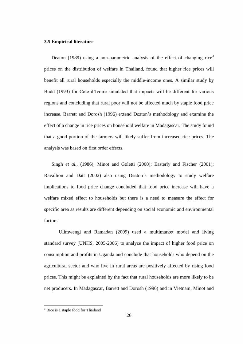
3.5 Empirical literature
Deaton (1989) using a non-parametric analysis of the effect of changing rice3
prices on the distribution of welfare in Thailand, found that higher rice prices will
benefit all rural households especially the middle-income ones. A similar study by
Budd (1993) for Cote d’Ivoire simulated that impacts will be different for various
regions and concluding that rural poor will not be affected much by staple food price
increase. Barrett and Dorosh (1996) extend Deaton’s methodology and examine the
effect of a change in rice prices on household welfare in Madagascar. The study found
that a good portion of the farmers will likely suffer from increased rice prices. The
analysis was based on first order effects.
Singh et al., (1986); Minot and Goletti (2000); Easterly and Fischer (2001);
Ravallion and Datt (2002) also using Deaton’s methodology to study welfare
implications to food price change concluded that food price increase will have a
welfare mixed effect to households but there is a need to measure the effect for
specific area as results are different depending on social economic and environmental
factors.
Ulimwengi and Ramadan (2009) used a multimarket model and living
standard survey (UNHS, 2005-2006) to analyze the impact of higher food price on
consumption and profits in Uganda and conclude that households who depend on the
agricultural sector and who live in rural areas are positively affected by rising food
prices. This might be explained by the fact that rural households are more likely to be
net producers. In Madagascar, Barrett and Dorosh (1996) and in Vietnam, Minot and
3 Rice is a staple food for Thailand
27
Goletti (2000) using Deaton approach of NBR found that, in the short run, those who
are net buyers in the cities and in the rural areas are the most adversely affected.
Ivanic and Martin (2008) estimate the short run effects of higher food prices
for seven commodities on poverty using living standard survey in nine developing
countries. The study concluded that on average a 10 percent increase in food prices
leads to an increase in poverty. However, an analysis by product and by country gives
different results for instance in Zambia was found 10 percent increase in maize price
increases rural poverty by 0.8 percentage point and urban poverty by 0.2 percentage
points. The study conducted by Wodon et al., (2008) in Ghana, Senegal and Liberia
highlighted that rising rice prices adversely affects households’ income in the short
and long run, and increases poverty in most of the regions. Beyond the household
profile, some empirical results are explained by the social and economic situation of
each country and region.
There is evidence that in Malawi food price increase has asymmetric impacts
on poor and rich households. Taylor et al., (2003) using Deaton approach found that
the welfare increase was small among the positively impacted groups, the middle
income group and poor and better off were negatively affected. However the study did
not take into account income or expenditure per adult equivalent as a measure of
welfare.
Benfica (2012), on the welfare and distributional impacts of price shocks in
Malawi, using Compensating Variation and NBR found that urban households were
severely affected and in rural areas, relatively better off households were more
negatively affected and poorest suffered the most with food price increase. However,
the study could not gather detailed retrospective information on changes in specific
28
areas and specific food, often in a given region there are typically wide divergence in
standards of living.
Badolo (2012) highlighted that in Malawi, a 10 percent increase in maize price
increases rural poverty by 0.5 percentage points, and urban poverty by 0.3 percent
points respectively. Khonje (2008) found that among others, maize prices
significantly and positively influenced the rate of food price inflation in Malawi.
Karfakis (2008) found that as food price increases households would be vulnerable to
food leading to food insecurity.
According to FAO (2011) at macro level, most food importing countries will
be negatively affected by the food price increase and certain countries that export
food will be positively affected by food price increase. Controlling for other factors,
countries with lower income will be highly affected. At micro level the effect will
vary geographically and depend on household population and whether the household
is a net buyer or net producer of that particular food.
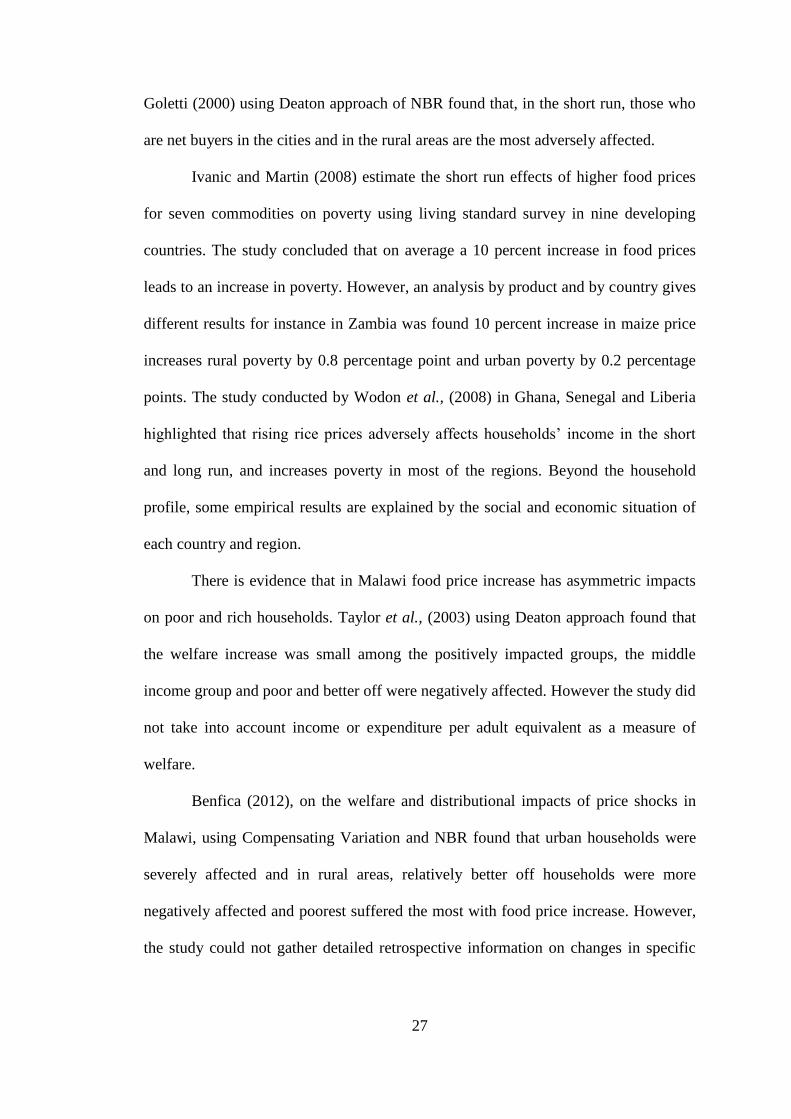
3.6 Conclusion
The chapter has reviewed theories and different studies on welfare change to
commodity price increase. However, studies have revealed that there are variations in
vulnerability depending on location, livelihood and other socioeconomic and
environmental factors which also give relevance of this study. The next chapter
presents the methodology used in the study; the empirical model, analytical methods
and data sources.
29
CHAPTER FOUR
METHODOLOGY
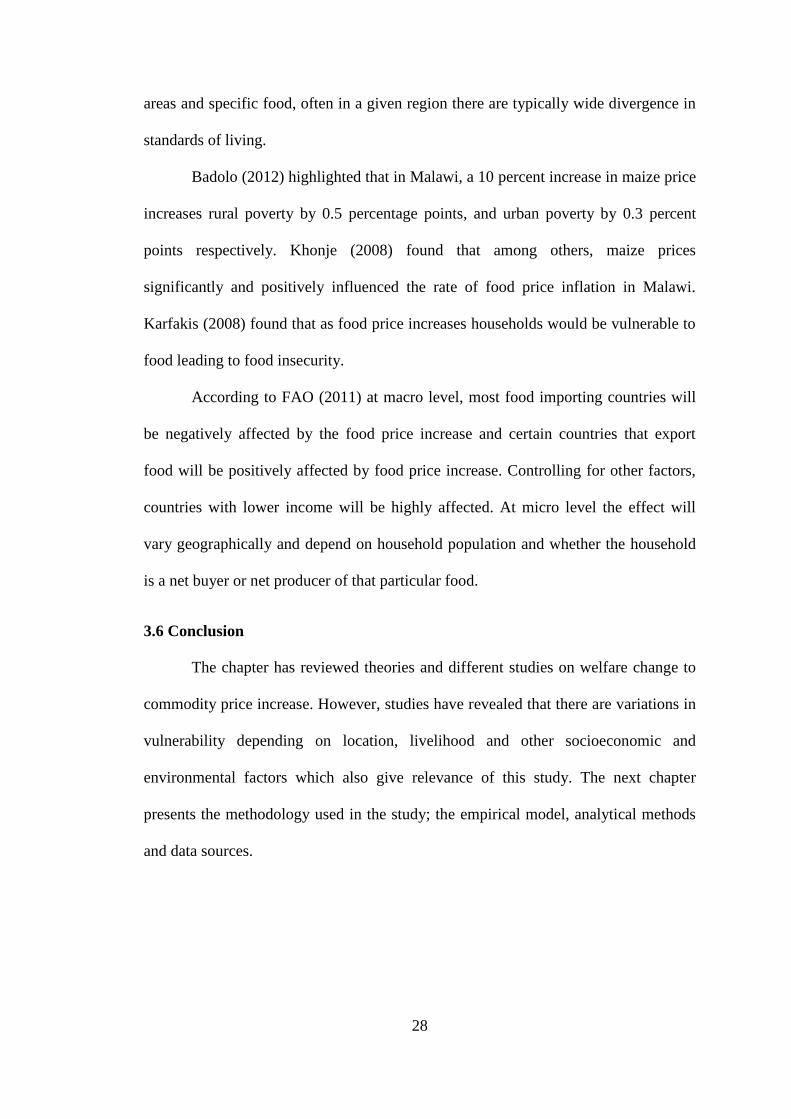
4.0 Outline
This chapter presents the methodology of the study. It is organized in six
sections. The study uses primary data. Section 4.1 presents research design, section
4.2, the analytical framework and modeling specification. Description of the
variables, data analysis and secondary data source are presented in section 4.3, and
methodological assumptions are in section 4.4. Section 4.5 presents the correction of
errors and lastly section 4.6 concludes the chapter.
4.1 Research Design
The study employes the Individual Household Method (IHM)4 in order to simulate the
income gain and loss as a measure of welfare of rural households in
Masumbankhunda and Mtimaukanena in Lilongwe and Dowa district respectively.
The model allows for simulation of distributional effect and individual household
effects on disposable income. This was achieved by collecting information on income
4 Visit: www.evidencefordevelopment.com

30
from five different sources and also information on consumption from own
production for the household.
4.1.1 Data Collection Method and Sampling design
A multi-stage sampling design was used where both purposive and random
samples were drawn to select the villages. The first stage involved a purposive
selection of Kasungu-Lilongwe plain area which covers these districts: Kasungu,
Dowa, Lilongwe, Mchinji Ntchisi, Dedza and partially Mzimba south. The second
stage involved a random selection of two districts in Kasungu-Lilongwe plain. The
district social welfare office provided the list of Traditional Authorities (TAs) in each
district and their villages. In each selected district, one TA was randomly selected.
The fourth stage involved selection of villages in each selected TA. Two villages were
randomly selected from the list in each TA. Additional villages were selected as
alternative sample villages in case the selected villages did not meet the survey
criteria of being willing to participate in the study. More than 30 households in size in
each village were ideal for the study to reduce sampling size error.
Selected villages were visited in turn, village mapping was conducted. Each
household on the map was then numbered and in each village, all households which
met the study criteria were interviewed. In case where a household was found to be
vacant, the household was revisited. In a case where for some other reason a
household was unable to participate in the survey the household was not included in
the survey. The sample design was constrained by the need to allow the survey to be
completed with the number of interviewers and within the time available.

31
The village population was interviewed to limit the influence of outlier
observations due to household sample errors. The village with a population of at least
60 households met the sample design criteria because the aim was to obtain a sample
of more than 30 households. Sample size of 30 representatives is considered
minimum sample size for being statistically significant (Gujarati, 2003). A total of 72
households in Masumbankhunda and 53 households in Mtimaukanena were
interviewed.
The field assessment team comprised of graduates and post graduates from
Chancellor College and Bunda College, University of Malawi. The supervising staff
and all members of the field assessment team had prior experience of the interview
technique used.
The interview technique used has been developed over several years. In
summary this requires that: (i) the interviewer has a good working knowledge of the
local economy e.g. crop types and probable returns, employment opportunities,
seasonality, prices etc. (ii) questions are asked in a way which is likely to allow a
respondent to recall all sources of income e.g. for employment income this will
involve working through the year month by month, in some cases separately by
male/female/ family employment. (iii) interviews are short, typically less than 1 hour
in length and each interviewer conducts only a small number of interviews each day
(four on this survey) to avoid the deterioration in interview quality which results from
interviewer and respondent fatigue. (iii) The data was checked and verified ideally on
the day of collection, this allowed the household to be revisited if required.

32
Household interviews were related to the period, April 1st 2011 to March 31
st 2012, a
period selected to include the entire maize harvest in the 2011 – 2012 agricultural
year.
Each interview covered:
- Household membership, by age and sex, absentees (e.g. men working at a
distance) and the period of absence.
- Current school attendance,
- Household land cultivated in the reference year (categorised as lowland
dimba, upland dimba, upland and ‘domestic garden’ i.e. upland close to the
household residence) and the status of this land i.e. owned, rented.
- Holdings of major assets (the number of livestock by type, bicycle, radio,
significant agricultural equipment).
- Household income obtained during the reference year as food and money from
crops, livestock, employment, wild foods, ‘gifts’ and remittances. Gifts
include gifts from kin and external assistance e.g. from NGOs. For traded
items e.g. crop sales the actual price obtained was recorded.
- Any credit taken during the reference year, its source and the reason for taking
this.
- The agricultural inputs used, their source, quantity and price and their use i.e.
the percentage of all inputs applied to different types of land and crop.
33
The price of produce and labour sold by households was recorded on the survey for
each household and each transaction.
Conversion factors for local measures (e.g. plates to basins) to metric
measures were used. The conversion of food items to their food energy equivalent
was done using standard reference sources. Land areas were recorded in acres. In the
case of upland plots close to the household these were identified and the area
estimated by pacing.
Additionally, data was gathered from key informants like village elders and
active youth on their minimum consumption of paraffin, soap, clothes, school costs
includes uniform and school materials, house repairs, salt and household utensils. This
was used to establish a standard of living threshold. The threshold was set at a level
commensurate with social inclusion. Key informants also provided contextual
information, including crops grown in the village, average yield obtain for each crop,
if crop was sold minimum and maximum prices were obtain, means of transportation
to the market, main markets of farm produce. Focusing on maize the chain was
obtained from production to consumption. Key information on markets, prices and
yield by income group, farm inputs, livestock, employment, remittances, and wild
food were collected from focus group discussion and individual household.
At the end of each day the interview data was entered into the ‘open-IHM
1.5.1’ software, to allow the data to be reconciled and checked for inconsistencies.
Interview findings which were found to be inconsistent or were otherwise known to
be incomplete e.g. due to the absence of a household member, were then revisited. If
it was then found that the interview could not be completed that interview was
rejected.
34
4.2 Analytical Framework
To simulate the impact of changes in food prices on household welfare; in this
study the impact of price changes on household welfare is measured by the change in
disposable income. The IHM approach provides analysis of simulating the impact of a
shock and modeling household income, food security and poverty in the presence of a
shock.
4.2.1 Salient Features of the IHM Model
The IHM modeling approach has been developed from the Household
Economy Approach (HEA) and currently used by VAC to assess vulnerability. The
two approaches (HEA and IHM) are quite similar in that both approaches provide a
quantitative description of defined populations for example strategies that people
employ to access food and income. IHM uses household consumption levels as proxy
for income. The open-IHM software was designed for data checking and analysis; this
is needed as household data can be difficult to manage, and decision making requires
current information (Seaman and Petty 2010). IHM software is used to calibrate the
model and perform the simulations.
Analytical approach to estimate the welfare effect employed in this study is
similar to Deaton (1989) Ravallion (1989) and Minot and Goletti (2000)
conceptualization of food prices. The estimate of welfare effect is determined by
comparing how the shares of the main staple product (maize) in household
consumption and income vary following percent change in prices of the products and
they all assume zero elasticity to price change.
However there are significant departures from Deaton’s and in Minot and
Goletti’s approach. Unlike Deaton which uses concepts of compensating variation;
the amount of income needed to restore a household to its position prior to the income

35
shock of high prices, which uses the real income lost to high food prices and calculate
as percentage change in total consumption expenditure, the IHM methodology
employed in this study used more realistic concept of welfare measure; the disposable
income lost to high food prices and calculated as percent change in total consumption
of income earned by a household. Instead of using the NBR as in the Deaton, the IHM
uses adult equivalents like Chayanov (1966) on farm household model in order to
determine a household’s food and non-food needs.
Secondly, in IHM like in Chayanov (1966) there is a poverty line that
demarcates the household poverty by using income as an indicator. In IHM,
households are required to meet some set standard of living threshold modeled based
on primary data. Deaton (1989) and Minot and Goletti (1989) measure of welfare lack
household demographic structure at the centre of its analyses as IHM and Chayanov,
hence the welfare measure in Deaton is arbitrary because it is not clear how household
welfare is measured as argued by World Bank (2011) and FAO (2012). IHM measure
of poverty use standard of living threshold. The STOL in the IHM considers a
household’s basic needs in greater detail and hence is more reflective of the
household’s needs in a particular area of study.
Thirdly, the IHM recognizes five sources of income and these are crop
production, livestock, employment, wild foods and transfers. IHM uses income which
is close to realistic measure for welfare. On this backdrop, the IHM provides a more
accurate measure of welfare using income as an indicator of poverty. Finally the IHM
recognizes the existence of local institutions and their play in supporting the
households through transfers and does not make any restrictive assumption on food
market. The centre of analysis and household assumption used here, like in Deaton,
(1989) and Ravallion, (1989) is to distinguish between net seller (surplus producer)
36
and net buyer. The IHM is designed to measure impact of a shock. Hence the IHM
model is more versatile and more appropriate for this study.
4.2.2. Limitation of the Study Methodology
The results may be underestimates for households that spend substantial shares
of their income on other staple food like cassava. However in the study area maize is
by far a staple food commodity. This was also indicated by FAO (2008) and Hoyos
and Medvedev (2008) as a major limitation of many welfare impact simulations.
Second, it was not possible to use actual price changes in each household and study
area local markets as local market prices are highly volatile (affected by seasonality)
and do not always reflect national prices.
4.3 Model Specification
Economic theory posits that households can be both producers and consumers
of crops at the same time. For example, a rural household that grows maize on the
farm can both sell and consume maize. Unlike in urban many household tends to
purchase maize and few produce it. In rural areas price increases can benefit net-
sellers of crops but can hurt net-buyers of crops.
Impacts of a shock, in this thesis, high staple food prices on disposable
incomes and welfare depend on the demographic characteristics of households which
include age, sex, number of people in the household, sources of cash, food income of
a household and on the structure or balance of the economy as indicated by Evidence
for Development and World Bank, (2009).
Like Deaton (1989) and Ravallion (1989) the IHM is based on theory that
changes in food prices can affect poverty and inequality through consumption and
income channels. On the consumer side, as food prices increase, the monetary cost of

37
achieving a fixed consumption basket increases hence reducing consumer’s welfare.
IHM modeling of food price shock is based on household income and the model
specifies that high commodity price will have a positive income effect to surplus
producers (net sellers) household of that commodity and negative income effect to
deficit producers (net buyers) household of that commodity. Hence in IHM, the net
welfare depends on contribution of the commodity to household income, household
sources of income and whether the household is a deficit or surplus producer of
maize.
To implement this framework, this study using IHM uses household
disposable income per adult equivalent as a measure for welfare and the household
ability to meet food needs and non-food as a measure of poverty. In IHM the sources
of income in a rural setting are considered to be crops, livestock, employment, wild
foods and transfers. Below is a specification of the disposable income per adult
equivalent function;
AEFCPYMYAEDI ffc // (4.1)
Where:
Income Disposable =DI
AE= Adult equivalent
(Kcal)t requiremen food HouseholdM
(Money) incomecash Household =cY
(Kcal) Household by the consumed income food Household = Y f
Kcalfood/ of Price = Pf

38
householdin sequivalentadult / erms)monetary t(in costs fixedother = FC
Total household cash income sum of each cash income source adjusted for
changes in price and production.
Total household food income consumed by the household (Kcal) sum of
each food income source adjusted for changes in production.
Total household food requirement the sum of the energy requirements of
each household member calculated by age and sex
The price of food is the diet; if more than one food is purchased the weighted
price per kilocalorie is used.
Other fixed costs are usually zero as there are not any, but worth mentioning
as occasionally people do have to pay tax, rents; in which case it is subtracted.
Because the price of food may be changed, also the food requirement, non-
food costs etc may be changed
4.4 Data Analysis
Data was analyzed using Open-IHM version 1.5.1. The study apply IHM
model to evaluate the effect of rising maize prices by introducing a shock on prices
for maize. Based on the background discussion, the study increases the prices of
maize by 80 percent. 80 percent is the price change reported by MoAFS within the
reference year. Based on the assumptions first the study run a baseline and lastly, the

39
study run a simulation where all other factors apart from maize price change are
assumed constant.
4.4.1 Welfare Measures and Poverty Analysis
In this study per adult equivalent as a measure of poverty is selected because it
gives distribution effect for each household or quintile without being biased to
households with high income despite high dependency ratio compare to a household
with same income with low dependency ratio. Therefore allows comparisons to be
made if same income data can be collected in different livelihood zones, region and
countries.
4.4.2 Price Data
Price data of maize from 2010 to 2013 was obtained from Ministry of
Agriculture and food security5, and administrative data was collected from
ADMARC. The baseline data analysis used maize price data obtained from the study
area through focus group discussion. The key informants gave a minimum and
maximum price of 2011/2012 reference year and the average price was used.
Purchased food was maize at an average of MK 25 per kilogram in Masumbankhunda
and MK 40 per kilogram in Mtimaukanena. The average maize sale price recorded
were MK 40 per kilogram in Mtimaukanena and MK 25 per kilogram in
Masumbankhunda. The variation presumably reflecting the difference in location of
study areas and the sale for instance trade within villages were at much lower prices
than at trading centres and prices immediately after the harvest and during maize
scarcity were highly varying, hence the use of average prices.
5 Price data is available at www.moafsmw.org

40
4.5 Presentation of Results
Rural households obtain their income as cash from employment, cash gifts and
the sale of food and non-food production and other income in kind and as food from
their own crop and livestock production, gifts and payment in kind, hunting and
gathering, payment in kind. As there is no market for some produce e.g. wild foods,
some livestock production or prices vary substantially between transactions; food
income cannot be consistently converted to its cash value (Seaman et al., 2008).
Therefore the results have been presented as household ‘disposable income’.
4.5.1 Baseline
The purpose of this analysis is to compare the case if prices were not changed
at all, what would be the actual disposable income per adult equivalent in each
household that can be affected to the price changes. In this case the study assumes that
for all the crops prices remain the same during the period. The study also assumes that
total factor productivity growth is one percent. These assumptions are used through
all baseline and other simulations.
4.5.2 Simulation
The purpose of this simulation is to compare the case, given maize prices
change by 80 percent ceteris paribus, what would be the actual net gain or losses to
welfare that can be attributed to the price changes. In this case the study assumes that
for all the crops expect maize prices remain the same during the period. The study
increases the price of maize by 80 percent in the year 2011/2012. The study assumes
that this increase is a one-off spike that does not adjust back to the earlier levels
(permanent increase) or this increase in the maize price is not temporary.
One would argue that, in essence this is a more unrealistic scenario since
prices of maize in Malawi start to drop in some months, however the MoAFS reported

41
a marginal drop in price of maize even in local markets throughout the year compare
to some months in the previous year and the price change used in the study is the
national price. Finally, for simplicity, the simulation assumes that price changes are
transmitted equally to different types of households, be they poor, middle, better off
consumers or buyers or sellers in the study area as assumed in many welfare
measures.
Simulation equation for 80 percent price increase;
If a household fails to meet its food requirement from own production,
simulation equation will be:
8.1** PQY pR 4.2
If a household meet all its food requirements from own production and have
surplus to sell, simulation equation will be:
8.1** PQY sI 4.3
Where:
RY = decrease in income
IY = increase in income
pQ = quantity purchases
sQ = quantity sale
P = price of maize
4.6 Description of Key Variables Considered in the Study
Welfare
This is the dependent variable; this study uses income as a proxy for poverty
or welfare. This variable is measured as a continuous number in cash (Malawi
Kwacha) and food in kilocalorie. The relationship between income and maize price
42
change can be positive, neutral as well as negative. The relationship comes in the
sense that in rural areas households are likely to be both producers and consumers of
maize. The net maize seller household will face a profit effect and a net buyer
household- a household which produce less and face own food production deficient
and relying on consuming from maize market purchases will have a negative income
effect due to a shift in income or real income effect.
Poverty
Poverty is pronounced deprivation in well-being, and comprises many
dimensions. In this thesis a household is regarded living below the standard of living
threshold (STOL) if it fails to meet both food and non-food expenses. Absolute
poverty is defined as the lack of sufficient resources with which to keep body and soul
together. Relative poverty defines income or resources in relation to the average. It is
concerned with the absence of the material needs to participate fully in accepted daily
life.
Net buyer and Net seller household
In this thesis a household is regarded as a net buyer if it fails to meet its food
requirement from own production. A net seller household is a household that meet all
its food requirements from own production and have surplus to sell.
Dependency Ratio
Age dependency ratio is equal to ratio of persons in the ‘dependent
ages’(under 15 and over 65) to those in the economically productive ages.
(number of people aged 0 - 14) + (number of people aged 65+)(Total ) Dependency ratio =
number of people aged 15 - 64
43
Sex ratio
Sex ratio is ratio of males to females in a given population, usually expressed
as number of males for every 100 females.
Household size
The mean household size is calculated as the ratio of the total household
population to the number of households in an area.
Age of Household head
The mean age of household head is calculated as the ratio of the total age of
household head to the number of households in an area. To avoid biases that occur
when mean is used, median age was also analyzed. Median age was age at which
exactly half the age of household head by income quintile is older and half is younger.
Disposable Income
In IHM disposable income is defined as the cash income remaining after the
household has met its food energy requirement at a specified level, either from its
own production or when this is insufficient by food purchase. In this calculation the
food energy requirements used are the UN requirements by age and sex for a
population of a typical developing country.
Household income
IHM categorises income into food and cash income. Food income is obtained
from consumption of own produced crops and livestock products, wild foods and food
received as a gift and payment in a form of food.
In additional, to undertake the analysis, the study needed the following
variables; households own production consumed directly (has a value and would
otherwise be bought), own-consumption and sales of agricultural products. Food and
commodities earned, for instance through labour, and if consumed directly, food aid
44
and other handouts consumed, cash earnings from all members of a household (crops,
labour, petty trading, collections and sale of assets), wild food consumed like hunting.
4.7 Some Methodological Issues
Additional assumptions in the methodology;
− Households receive their income from primary factor payments. They also
receive transfers from government and the rest of the world.
− Households pay income or rent in labour and these are proportional to their
incomes.
− Savings and total consumption are assumed to be a fixed proportion of
household’s disposable income (income after non-food expenses).
− Regarding the elasticity, most of the studies assume no household responses
(e.g. Deaton, 1989; Ivanic and Martin, 2008), this means that the elasticity are
equal to zero or homogenous to degree zero this is also assumed in this study.
− Consumption demand is determined by household demography and its total
production. Households receive their income from remuneration of capital
assets; which include human capital, physical capital, social capital, financial
capital and natural capital
− Household expenditure is equivalent to household income ( ye )
− Savings are equivalent to investments ( is ) and assumes that investments in
the current period are used to build on the new capital stock for the next
period.
− The model has no restrictive assumption on market

45
4.8 Equivalence Scales
The choice of a poverty line and the associated poverty measure is important
in poverty measures (World Bank, 2012). According to World Bank (2009) poverty
measures based on per capita welfare indicators may not be good estimates. An
alternative is to base poverty measures on expenditure (or income) per adult
equivalent; therefore the study adopted this by using per adult equivalence scale.
4.9 Counter Factual Analysis
IHM conducts counterfactual analysis. This counter factual analysis considers
two scenarios i.e. scenario with impact and scenario without impact. This analysis is
commonly referred to as the “with” and “without” analysis. In this case, what would
households be without a change in price was a “without” scenario, analyzed with
baseline data and after model simulation the analysis gives “with” scenario. The
household incomes collected in the survey were treated as incomes in the “without”
scenario. Comparisons were made between the “with” and “without” scenarios to
assess the effect of the maize price increase on a household.
4.10 Correction for errors
There are two main types of errors: sampling errors and measurement errors.
The study used population census method; all households in the selected villages were
interviewed. This method removes selectivity bias. Measurement errors were reduced
by the data collection technique. Disposable incomes and household consumption was
a proxy for income, adult equivalents as a measure also removed some biases. The
standardization that was adopted also helped to address heteroscedasticity which is a
likely problem when dealing with primary data. IHM software used check for
completeness and consistency in the data. Data was checked on the same day of data

46
correction and data entry. The basic output chart was produced the same day which
allows follow up for missing information on the following day as income data need
checking for consistency. Interviewers were well trained on income data collection,
checking, observing and probing while collecting household information.

47
CHAPTER FIVE
EMPIRICAL RESULTS AND ANALYSIS
5.0 Outline
This chapter presents the results and analysis of the methods outlined in the
previous chapter. In this analysis MK140 is equivalent to $1. The chapter is presented
in four sections. Section 5.1 presents the results from focus group discussion, section
5.2 demographic and socio-economic findings followed by descriptive statistics.
Section 5.3 presents simulation analysis and interpretation. Finally, section 5.4
concludes the chapter.
5.1 Brief of Focus Group Discussion
The major sources of livelihood in both villages were farming. However, there
were some off-farm activities such as butchery, selling crops as traders, bicycle hire,
petty trade, beer brewing and charcoal selling. The households regarded better off
were growing different types of crops including cash crops and were using fertilizer
and other inputs in their fields. These households were involved in hiring in labor and
had different types of assets including radios, oxcarts and bicycles and on average rich
households were keeping large herd of livestock compared to poor households. Many
households in the poorest category engaged in hiring out agricultural labour especially
in agricultural season which reduces productivity in

48
their own farms. On average the poorest households did not use adequate inputs in
their fields.
Major crops were maize, cotton, tobacco and ground nuts in the villages. The
villagers were selling maize locally at lower prices which is called farm gate price to
individual households and vendors. Some were selling at nearest formal and informal
markets. On average, selling and buying prices for crops were not varying by wealth
status. Lumbadzi about 18 kilometers away from Mtimaukanena village was the main
market for maize. Chigwirizano about 9 kilometers away from Masumbankhunda
village was the main market for maize. In order to get an overview of demographic
and socio-economic position of these villages, section 5.2 presents demographic and
socio economic characteristics.
5.2 Socio-Economic and Demographic
The variables assessed include population of people from interviewed
households, age and sex distribution, sex ratio, dependency ratio, median age by
income quintile, age of household head, household size and sex of household head in
percent by income quintile.

49
Table 5.1: Age and Sex distribution
Mtimaukanena village
Age Group Male Female Sex ratio
0 to 4 15 18 83
5 to 9 29 21 138
10 to 14 14 15 93
15 to 19 21 9 233
20 to 24 11 10 110
25 to 29 10 10 100
30 to 34 10 11 91
35 to 39 9 3 300
40 to 44 1 2 50
45 to 49 0 6 0
50 to 54 3 3 100
55 to 59 3 2 150
60 to 64 6 6 100
65 to 69 3 1 300
70 to 74 2 4 50
75+ 3 1 300
Population 140 122 115
Total 262
Masumbankhunda village
Age Group Male Female Sex ratio
0 to 4 14 21 67
5 to 9 22 29 75
10 to 14 35 22 159
15 to 19 18 10 180
20 to 24 10 13 77
25 to 29 10 18 56
30 to 34 11 4 275
35 to 39 14 8 175
40 to 44 9 5 180
45 to 49 5 4 125
50 to 54 2 5 40
55 to 59 6 2 300
60 to 64 0 3 0
65 to 69 2 4 50
70 to 74 0 2 0
75+ 4 2 200
Population 162 152 107
Total 314
Source: Own computations based on IHM data

50
Population
Table 5.1 indicates that population distribution was such that; Mtimaukanena
village had 262 people from 53 interviewed households while Masumbankhunda
village had 314 people from 67 interviewed households. In Mtimaukanena 136 people
(52 percent) were aged between 15 and 64. In Masumbankhunda157 people (50
percent) were aged between 15 and 64. This shows that 52 percent of the population
in Mtimaukanena and 50 percent of the population in Masumbankhunda was
economically productive.
Sex ratio
The sex ratio was 115 in Mtimaukanena and 107 in Masumbankhunda. This
indicates a higher number of male to female in both villages. Population of under-five
had sex ratio of less than 100 in both villages indicating that, in infant population the
female population exceeded the male population, 83 percent in Mtimaukanena and 67
percent in Masumbankhunda (Table 5.1).Mtimaukanena had high sex ratio compare
to Masumbankhunda. High sex ratio implies more male to female. In both villages the
ratio of more than 100 was observed in many age groups.
In Mtimaukanena six out of 16 age groups had female population exceeding
male. These age groups are: (0 to 4), (10 to 14), (30 to 34), (45 to 49) and (70 to 74)
while in Masumbankhunda seven out of 16 age groups had more female to male
population. Below is Figure 5.1 (population pyramid of two villages) illustrating these
findings.
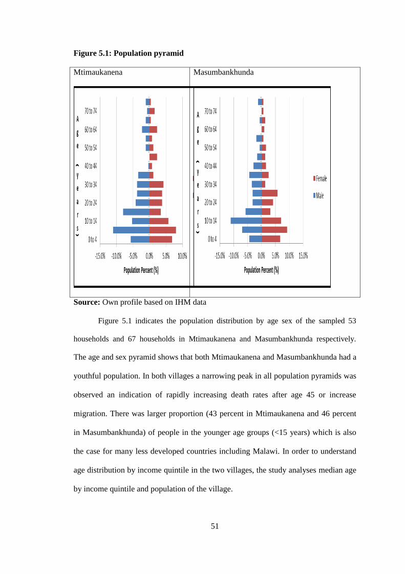
51
Figure 5.1: Population pyramid
Mtimaukanena
Masumbankhunda
Source: Own profile based on IHM data
Figure 5.1 indicates the population distribution by age sex of the sampled 53
households and 67 households in Mtimaukanena and Masumbankhunda respectively.
The age and sex pyramid shows that both Mtimaukanena and Masumbankhunda had a
youthful population. In both villages a narrowing peak in all population pyramids was
observed an indication of rapidly increasing death rates after age 45 or increase
migration. There was larger proportion (43 percent in Mtimaukanena and 46 percent
in Masumbankhunda) of people in the younger age groups (<15 years) which is also
the case for many less developed countries including Malawi. In order to understand
age distribution by income quintile in the two villages, the study analyses median age
by income quintile and population of the village.
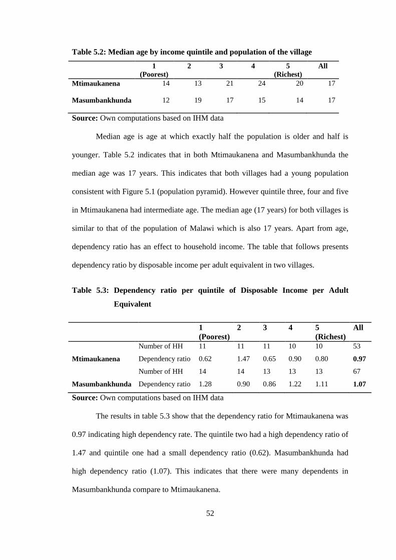
52
Table 5.2: Median age by income quintile and population of the village
1
(Poorest)
2 3 4 5
(Richest)
All
Mtimaukanena 14 13 21 24 20 17
Masumbankhunda 12 19 17 15 14 17
Source: Own computations based on IHM data
Median age is age at which exactly half the population is older and half is
younger. Table 5.2 indicates that in both Mtimaukanena and Masumbankhunda the
median age was 17 years. This indicates that both villages had a young population
consistent with Figure 5.1 (population pyramid). However quintile three, four and five
in Mtimaukanena had intermediate age. The median age (17 years) for both villages is
similar to that of the population of Malawi which is also 17 years. Apart from age,
dependency ratio has an effect to household income. The table that follows presents
dependency ratio by disposable income per adult equivalent in two villages.
Table 5.3: Dependency ratio per quintile of Disposable Income per Adult
Equivalent
1
(Poorest)
2 3 4 5
(Richest)
All
Number of HH 11 11 11 10 10 53
Mtimaukanena Dependency ratio 0.62 1.47 0.65 0.90 0.80 0.97
Number of HH 14 14 13 13 13 67
Masumbankhunda Dependency ratio 1.28 0.90 0.86 1.22 1.11 1.07
Source: Own computations based on IHM data
The results in table 5.3 show that the dependency ratio for Mtimaukanena was
0.97 indicating high dependency rate. The quintile two had a high dependency ratio of
1.47 and quintile one had a small dependency ratio (0.62). Masumbankhunda had
high dependency ratio (1.07). This indicates that there were many dependents in
Masumbankhunda compare to Mtimaukanena.

53
To gain an insight of household characteristics in two villages, the study
further analyzed mean household size, age of household head, sex of household head
and household assets. Next is the table presenting these variables by income quintile
and village population.
Table 5.4: Demographic characteristics of households by income quintile
Source: Own computations based on IHM data
a Average (Avg.), b Median (Md), c Male (m), d Female (f)
Income quintile
1 (Poorest) 2 3 4 5 (Richest) All
Mtimaukanena Number
of HHs
11 11 11 10 10 53
Masumbankhunda 14 14 13 13 13 67
Mtimaukanena
Masumbankhunda
Mean
HH size
5
5.21
6.18
4.85
4.45
5
3.9
4
5.4
4.38
4.79
4.70
Avga Mdb Avg Md Avg Md Avg Md Avg Md Avg Md
Mtimaukanena Age of
HH
head
41 33 45 37 49 38 50 39 49 53 49 53
Masumbankhunda 38 38 52 46 46 48.5 36.9 31.5 37.8 31.5 42.2 38.5
mc fd m f m f m f m f m f
Mtimaukanena Sex of HH
head (%)
73 27 45 55 70 30 90 10 100 0 67 23
Masumbankhunda 79 21 86 14 85 15 46 54 69 31 66 34
Average land cultivated by type and income quintile Md
Mtimaukanena Dimba (Acre) 0.07 0.12 0.4 0.3 0.4 0.27 0.24
Masumbankhunda 0.66 0.7 0.48 0.67 1.45 0.73 0.5
Mtimaukanena Upland (Acre) 1.4 1.34 2 1.5 4.4 2.1 1.7
Masumbankhunda 1.79 2.9 1.58 2.38 3.27 2.37 2

54
Age of Household head
Table 5.4 indicates that the average age of household head was 49 in
Mtimaukanena and 42 in Masumbankhunda. Average age of household head varies
across income quintiles. Average age of household head in Mtimaukanena was high
in quintile four and in Masumbankhunda was high in quintile two, 50 and 52 in that
order. In terms of median age, in Mtimaukanena median age of head of household
was 53 while in Masumbankhunda median age of head of household was about 39.
This indicates that there was a large difference in age of household head in the two
villages.
Sex of Household head
Table 5.4 indicates that in Mtimaukanena 23 percent of households are headed
by women. The figure (23 percent) is similar to national findings in Malawi country
profile of 2011. In Mtimaukanena the highest percentage of female headed household
was found in quintile two, 55 percent. In Masumbankhunda 34 percent of households
are headed by women. The highest percent of female headed household was found in
quintile four, 54 percent and all quintiles had at least a woman heading the household
unlike in Mtimaukanena where quintile five had no woman headed household. Results
indicate that, female-headed households are more prevalent in Masumbaknhunda than
in Mtimaukanena. The difference in female headship between Mtimaukanena and
Masumbankhunda might be due to the out-migration of men from Masumbankhunda
to urban areas such as Lilongwe town ship, due to its closeness to Lilongwe town
ship.
Household Size
The average household size in Mtimaukanena was 4.79 and the results indicate
average household size was higher in quintile two (6.18) and small in quintile four

55
(3.9). Masumbankhunda had an average household size of 4.7 and the higher average
household size was 5.21 in quintile one and small average size 4.38 in quintile five
(Table 5.4).
Household Assets
The welfare of households also depends on the asset base. Average ownership
land can have effect on production. Table 5.4 indicates the average area of land
cultivated in the reference year by disposable income quintile. The average area of
upland cultivated in Mtimaukanena was 2.1. The average area of dimba cultivated
was 0.27. The median area for upland was 1.7 and for dimba was 0.24. The average
area of upland cultivated in this village was far much higher in quintile five with an
average area of 4.4 acres. The average area of upland cultivated in Masumbankhunda
was 2.7. The median area for upland was 2 and for dimba was 0.5.The average area of
dimba cultivated was 0.73. Household regarded richest in the village owned large
piece of upland, average of 4.4 acres in Mtimaukanena and 3.27 acres in
Masumbankhunda from median of 1.7 acres and 2 acres respectively. The quintiles
one to four had an average of less than 1 acre cultivated dimba land.
In order to get an overview of main sources of livelihood in the two villages,
the section that follows, section 5.2.1 presents descriptive statistics of key variables
and various sources of household income.
5.2.1 Descriptive Analysis of the Data
Table 5.5 shows the descriptive statistics of the main variables used in the
study. It outlines the means, standard deviation, minimum and maximum observations
of the variables under study.

56
Table 5.5: Descriptive Statistics of Income by Source in Malawi Kwacha and
Kcal, Mtimaukanena
Variable Obs Mean Std. Dev. Min Max
Income by Source in Malawi Kwacha (MK) per Year
Mtimaukanena Cash
from crop
53 18,674.9 32019.9 0 147, 023
Masumbankhunda 67 52,522.19 72,230.4 0 337,112.8
Mtimaukanena Employment 53 86,652.8 123087 0 555, 000
Masumbankhunda 67 122,385.3 245,516.2 0 1,616,000
Mtimaukanena Livestock 53 8468.87 28714.3 0 204, 000
Masumbankhunda 67 8,457.015 14,858.92 0 77,900
Mtimaukanena Transfer 53 1592.45 9361.54 0 66, 800
Masumbankhunda 67 6,121.642 25,699.57 0 180,000
Mtimaukanena Wild food
(hunting)
53 1532.27 10571.8 0 77, 000.40
Masumbankhunda 67 0 0 0 0
Income by Source in Kilocalories (Kcal) per Year
Mtimaukanena Food from
Crop
53 2,851,344 2,802,402 141,066 17,629,865
Masumbankhunda 67 3,205,995 2,608,264 282960 13,759,994
Mtimaukanena Food from
employment
53 4,839.62 35,233 0 256,500
Masumbankhunda 67 17,865.67 146,236.8 0 1,197,000
Mtimaukanena Livestock
product
53 3,189.25 5,850.47 0 26,100
Masumbankhunda 67 7,816.209 13,990.75 0 79,470
Mtimaukanena Food from
Transfer
53 13,408.3 49,479 0 254,800
Masumbankhunda 67 22,386.88 75,375.54 0 406,850
Mtimaukanena Wild Food
(hunting)
53 36,141.5 133,152 0 967,540
Masumbankhunda 67 7,227 7,732.84 0 41,788
Mtimaukanena Baseline
DIa (MK)
53 33,076.2 40,082.5 -5878.7 156,617.6
Masumbankhunda 67 56,989.58 86,268.29 593.78 456,699.9
Source: Own computations based on IHM data
57
a Disposable Income (DI)
Income by Source in Mtimaukanena
Table 5.5 indicates that Baseline Disposable Income (DI) has a mean value of
about MK 33,076.2. This implies that the average disposable income per adult
equivalent before maize price increase was MK 33,076.2 per year. The variable also
has a standard deviation of approximately 40,082.5, which shows that there was a
wide range among the high income and low income households. This can be seen
from the range which is between MK -5,878.7 and MK 156,617.6 disposable incomes
per adult equivalent per year, implying some households had more income than
others. The nagitive sign implies household had a deficit of MK 5,878.7 inorder to
meet recommended food requirement.
A quick look at the sources of income indicates that, selling of crops had a
mean value of MK 18674.9. This implies that the average earning from crop is MK
18,675 per year. The variable also has a standard deviation of approximately
32,019.9, which shows that there was a wide range among the high earners and low
earners. This can be seen from the range which is between 0 and 143, 023 Malawi
Kwacha per year.
Employment was the major source of income for households in the village.
The average earning was MK 86,652.8. The variable has a standard deviation of
123087, which shows that there was a wide range among the low income households
and high income household. The employment cash income ranges from 0 to 555,000
Malawi Kwacha per adult equivalent per year. Livestock selling was coming third. In
this village 93 percent of households earned cash income from employment and 85.7
percent of households earned cash income from crop selling. Food income was
mainly from crops. Crop food income ranges from 141,066 Kilocalorie to 17,629,865

58
Kilocalorie per year. Other sources of food income such as livestock, transfers, wild
food and food from employment did not contribute much kilocalorie as shown in the
table.
Income by Source in Masumbankhunda
Table 5.5 indicates that Baseline Disposable Income had a mean value of
about MK 56,989.58. This implies that the average disposable income per adult
equivalent before maize price increase was MK 56,989.58 per year. The variable had
a standard deviation of approximately 86268.29, which showed that there was a wide
range among the high income and low income households. This can be seen from the
range which is between 593.78 and 456,699.9 Malawi Kwacha disposable incomes
per adult equivalent per year, implying some households had more income than
others. The lowest dispsable income per adult equivalent is positive, MK 593.78
implies that all households were above the poverty line.
Employment was the major source of income for households in the village.
Employment cash has a mean value of about MK 122,385.30. This implies that the
average, earning from employment is MK 122,385.30 per year. The variable also has
a standard deviation of approximately 245516.2, which shows that there was a wide
range among the high earners and low earners. This can be seen from the range which
is between 0 and 1,616,000 Malawi Kwacha disposable incomes per adult equivalent
per year, implying some households earn more than others. Crop was the second
major source of income with a mean of 3,205,995 Kilocalorie per year. Livestock
selling was coming third.
In this village the lowest baseline disposable income of MK 564.48, close to
zero line indicates that in the presence of external negative shock the households are
likely to fall below the poverty line.

59
Sections 5.1, 5.2 and 5.2.1 reveal that both Mtimaukanena and
Masumbankhunda had a youthful population with median age of 17 years.
Masumbankhunda had a high dependency ratio compare to Mtimaukanena, however,
on average there was not much difference in household size in the two villages.
Masumbankhunda had relatively large piece of cultivated upland compare to
Mtimaukanena. In terms of disposable income, on average, Masumbankhunda had
high disposable income per adult equivalent compare to Mtimaukanena. Employment
was the major source of income for households in both villages. Further analysis
follows in the next section. The next section presents contribution of maize to
household income in the two villages.
5.2.2 Contribution of Maize Income to Household Income
In order to get an insight of the modeling effect of changes in welfare through
household income as a result of maize price change, it is important to understand the
contribution of maize in cash and food to household income. The findings are
presented by quintile. The quintiles were categorized into five groups representing 20
percent of households’ wealthy group in the village. Quintile one means the lowest
(poorest) income group, quintile two lower-mid, quintile three middle, quintile four
mid-upper and quintile five highest (richest) income group in the village.

60
Figure 5.2: Contribution of Maize to Household Cash Income by income quintile,
Malawi Kwacha, Mtimaukanena
Source: Own profile based on IHM data
Figure 5.2 indicates that in quintile five households earned MK 275,425 from
maize selling and MK 3,347,999.60 from other sources of cash income. This implies
that about 8 percent of cash income in this quintile was earned from maize selling.
Quintile four earned MK 21,400 (2 percent) from maize selling and MK 1,132,539.75
from other sources of cash income. In quintile three maize cash income was MK
66,262 (9 percent) and other sources of cash income was MK 734,852.12. Quintile
one, maize cash income was MK 6,844 and other sources of cash income was MK
249,367.62. This implies about 2 percent of cash income in this quintile was obtained
from maize selling.
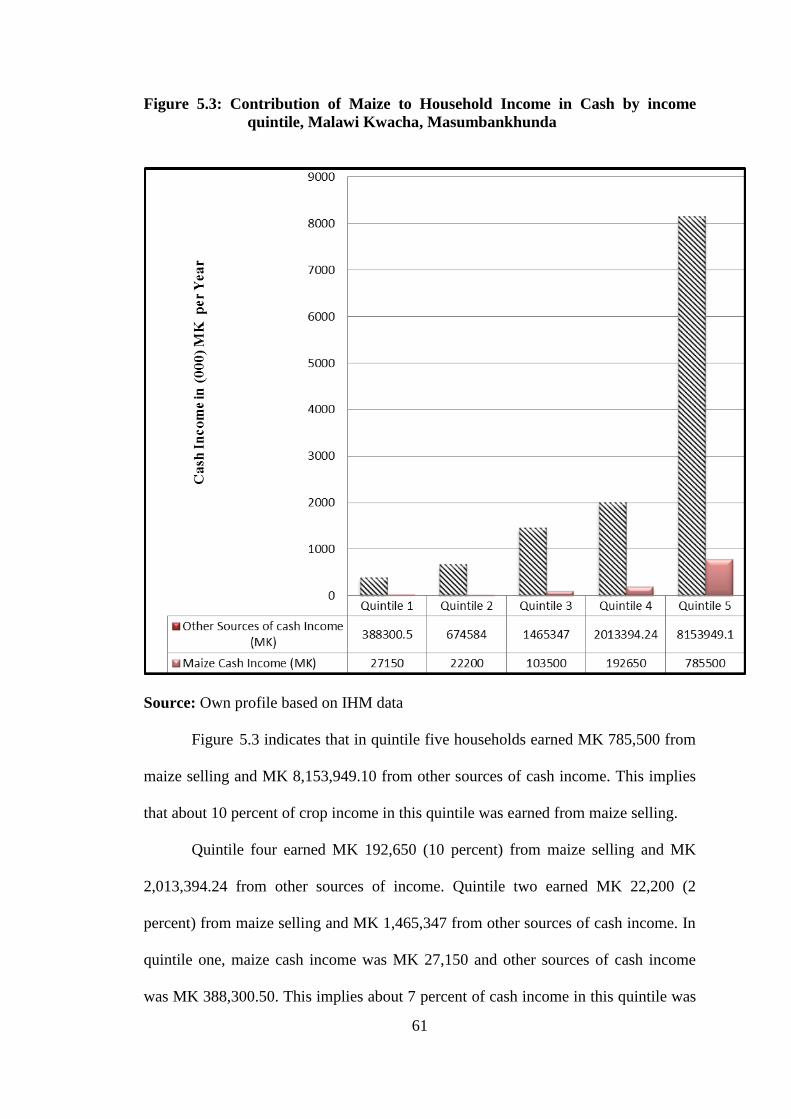
61
Figure 5.3: Contribution of Maize to Household Income in Cash by income
quintile, Malawi Kwacha, Masumbankhunda
Source: Own profile based on IHM data
Figure 5.3 indicates that in quintile five households earned MK 785,500 from
maize selling and MK 8,153,949.10 from other sources of cash income. This implies
that about 10 percent of crop income in this quintile was earned from maize selling.
Quintile four earned MK 192,650 (10 percent) from maize selling and MK
2,013,394.24 from other sources of income. Quintile two earned MK 22,200 (2
percent) from maize selling and MK 1,465,347 from other sources of cash income. In
quintile one, maize cash income was MK 27,150 and other sources of cash income
was MK 388,300.50. This implies about 7 percent of cash income in this quintile was

62
obtained from maize selling. The table below summarises the findings from Figure
5.2 and 5.3 above, of the contribution of maize to household total cash income.
Table 5.6: Contribution of Maize to Total Cash Income by Income quintile,
Malawi Kwacha
Source: Own computations based on IHM data
Summary from Table 5.6 indicate that in both villages maize contributed to
household cash income. In Mtimaukanena, in quintile three maize contributed high
percentage of cash income, 9 percent compare to other quintiles. The contribution of
maize in quintile one and four were the same, 2 percent. In Masumbankhunda the
poorest group generate a good percent of their income from maize selling about 7
percent equivalent to what is generated by the middle income group, quintile three.
Results in two villages indicate all quintiles were involved in maize selling. This
implies that increase in maize price can result to positive income effect to households
in these quintiles.
The profit and income effect are observed in illustration of Figure 3.1 and 3.2,
section 3.1 in chapter Three. The net position will depend on maize contribution to
cash (MK) and food (Kcal) from own production. Therefore further insights can be
Maize Cash Income (MK) Percent Contribution of Maize
to Total Cash Income
Household
Category
Mtimaukanena Masumbankhunda Mtimaukanena Masumbankhunda
Quintile Five 275,425 785,500 8 10
Quintile Four 21,400 192,650 2 10
Quintile Three 66,262 103, 500 9 7
Quintile Two 11,870 22,200 1 2
Quintile One 6,844 27,150 2 7

63
gained when we analyse the data in terms of relative contribution of maize in each
household group to gross food income in kilocalories by quintile.
Figure 5.4: Contribution of Maize Food Income to Total Food Income Consumed
(Total Energy in Kilocalorie), Mtimaukanena
Source: Own profile based on IHM data
Figure 5.4 indicates that in quintile two, three and four in Mtimaukanena,
maize is contributing 2,933,726 Kilocalorie, 2,717,140 Kilocalorie, 28,721,495
Kilocalorie in that order. In quintile five contributions of maize to food diet was much
higher 50,123,520 Kilocalorie. The quintile one, the poorest had 16,123,475

64
Kilocalorie from maize as compare to 25,650,094 Kilocalorie attained from other
crops igniting a difference of 9,526,619 Kilocalorie. This indicates that the poorest
household in this village rely much on maize food with little diversification
considering that other crop kilocalorie is a combination of any food produced by the
household from own production, hunting and received as gift including both crops
and livestock.
Figure 5.5: Contribution of Maize Food Income to Total Food Income Consumed
(% of Total Food Energy), Masumbankhunda
Source: Own profile based on IHM data
Figure 5.5 indicates that in quintile five, maize was contributing 43,882,280
Kilocalorie while other foods were contributing 55,520,563.6 Kilocalorie. This gives
a difference kilocalorie of 11,368,283.6. In quintile four, maize is contributing
24,882,634 Kilocalorie while other foods are contributing 29,198,593.6 Kilocalorie
65
giving a difference food kilocalorie of 4,315,959.6. In quintile three, maize is
contributing 27,060,580 Kilocalorie while other foods are contributing 33,053,550.8
Kilocalorie giving a difference Kilocalorie of 5,992,971. The difference in kilocalorie
for quintile two and one was 3,788,740.4 Kilocalorie and 3,288,931.15 Kilocalorie
respectively. The results indicate that other foods are not consumed much in quintile
one and two. The slope of food consumption in kilocalorie by quintile in the figure is
positive showing that moving from poor to better off, the better off are consuming
much food from own production than the poor. This implies that there is a different in
food resource allocation to households and an indication of high deficit in maize
production moving from better off to the poor.
From Figure 5.4 and 5.5, it can be observed that the difference in food
kilocalorie between maize and other food is high in the highest and mid upper income
groups compare to mid low and lowest income groups. Consumer theory explains that
when price of normal good increase consumers real income will reduce. Assuming
maize is a normal good an increase in price in this case, will lead to income and
substitution effect illustrated in Figure 3.1 in chapter Three. Substitution effect is
observed in Figures 5.4 and 5.5 above in that, in two villages households have more
than 50 percent of their consumption from other crops with maize contributing less. In
theory, this may imply there is a utility gain in consuming other crops as well.
Depending on consumer preference the utility gain may be higher consuming those
other food commodities as compared to maize.
Consumers may have to forgo other food bundle and choose maize due to
budget constraints when it was sold at cheaper price hence increase in maize price
will have a substitution effect. Consumers can easily substitute to the food
commodities or crops which derive the same or higher utility when consumed

66
compare to maize food but have relatively cheaper or equivalent price to maize.
However, relatively consumption of maize is high in both villages. This is observed
from the difference between maize consumption and other food consumption,
specifically considering that other crops include livestock which has high kilocalorie
per kilogram. In additional all households rely on maize as the main source of food in
kilocalories. This gives an impression that in the study area maize is a Giffen good.
For a Giffen good there is no close substitute. This implies that substitution
effect may not be observed when prices of maize rise. Income effect is observed in
Figure 5.4 and Figure 5.5 the poor households are consuming less kilocalorie compare
to the better off. This may indicate that the poor have own food production deficit and
are net buyers. In order to cover the deficit, the household will buy maize from the
market. Increase in maize price will push their budget and hence a fall in real income.
Due to budget constraint the household will change consumption of food and non-
food items hence an income effect and change to welfare.
Since non-food items that a household will cut down to cater for staple food
expenses include basic commodities like school fees, paraffin, soap clothes, the
implication is a fall in welfare. A fall in welfare is also observed in a fall in budget
leading to a lower satisfaction obtained from a new combination of food and non-food
commodities illustrated in Figure 3.2. The quintile five and three in Figure 5.2 and
quintiles five and four in Figure 5.3 have a substantial share of their income from
maize selling. All things being equal households in these quintiles, maize price
increase will lead to a producer surplus, also known as profit illustrated in Figure 3.3,
Panel II, in section 3.1 of chapter Three.
From this discussion it can be concluded that the simulation outcome will
depend on the wealth status of a household and whether it is a net buyer or net seller

67
household. In order to comprehend the definition of net buyer and net seller
household defined in this study, presented next, is the household budget for a net
seller and a net buyer household. Table 5.7 shows the household budget of one of the
better off household which also has maize surplus to sell and the other is poorest
household with maize deficit and falling below poverty line and Standard of Living
Threshold (STOL). In the table household food energy requirement is calculated
using age, sex and number of people in the household.
Table 5.7: Household Budget for Selected Maize Food Surplus and Deficit
Producer
Variable Surplus Producer
(Net Seller household) Deficit Producer
(Net buyer household)
Household food energy requirement
(Kcal)
3248500 2536750
Household food requirement met from
own production (%)
100 63.25
Cost of food purchase to meet household
requirement (MK)
0 10300.72
Food deficit which can be afforded (%) 0 0
Cash remaining after food purchase
(MK)
535019.01 -5800.72
Cost of non-food expenses (MK) 33660 26760
Non-food expenses which can be met
(%)
100 0
Cash remaining after non-food expenses
(MK)
501359.01 -32560.72
Source: IHM output
Table 5.7 indicates two households. The household that was able to meet all
required percent of its energy requirement from own food production and one that did
not meet all required percent of its energy requirement from own food production.
Own food production include crops and livestock. Surplus producer had 100 percent
68
of household food requirement met from own production indicating surplus in staple
food from own production. This household is therefore a net seller if it has maize
surplus. Assuming no any other shock to the household, increase in maize price will
lead to gain in welfare. If there is no maize surplus to this household, maize price
increase will have no effect to the household.
On the other hand, net buyer household presented in Table 5.7 is a poor
household which met 63.25 percent of food from own production. Due to inadequate
cash income, the household could not meet its food deficit. This household had a
negative amount (MK-5800.72) of cash remaining after food purchase an indication
that it is not able to buy all food required for the household. The household can not
afford the non food expenses hence MK-32560.72 cash remaining after non-food
expenses. The negative sign of amount of cash remaining after food purchase MK-
5800.72 indicate that the household in below the poverty line. The negative sign of
amount of cash remaining after non food expenses, MK-32560.72 indicate that the
household is below the standard of living threshold (STOL).

69
Next, the study presents the wealth status in relation to net position of the
households. Thereafter the study presents simulation analysis and interpretation of the
results.
Table 5.8: Relationship between Maize Net Buying/Selling and Income Status
Income
quintile
Net Buyer Net Seller Total
N Percent N Percent N Percent
Mtimaukanena Quintile 1 11 100 0 0 11 100
Masumbankhunda 14 100 0 0 14 100
Mtimaukanena Quintile 2 11 100 0 0 11 100
Masumbankhunda 12 86 2 14 14 100
Mtimaukanena Quintile 3 3 27 8 73 11 100
Masumbankhunda 10 77 3 23 13 100
Mtimaukanena Quintile 4 1 10 9 90 10 100
Masumbankhunda 1 8 12 92 13 100
Mtimaukanena Quintile 5 1 10 9 90 10 100
Masumbankhunda 0 0 13 100 13 100
Mtimaukanena Total 27 51 26 49 53 100
Masumbankhunda 37 55 30 45 67 100
Source: Own computations based on IHM data
Table 5.8 indicate that in Masumbankhunda from quintile one to quintile four
there are a total of 37 maize net buying households6 showing that majority of
households are net buyers. On the other hand, majority of households, 25 households
representing 37 percent in quintile four and five are net sellers7. From these it shows
that price increase will benefit net sellers and adversely affect the net buyers.
Therefore it is likely to have mixed results. Similarly, in Mtimaukanena households
6 A household is regarded as a net buyer if it fails to meet its food requirement from own production.
7 Net seller household is a household that meet all its food requirements from own production and have
surplus to sell.
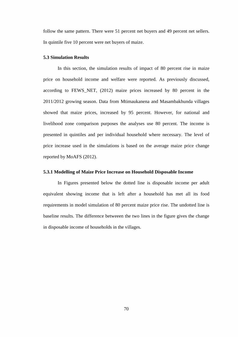
70
follow the same pattern. There were 51 percent net buyers and 49 percent net sellers.
In quintile five 10 percent were net buyers of maize.
5.3 Simulation Results
In this section, the simulation results of impact of 80 percent rise in maize
price on household income and welfare were reported. As previously discussed,
according to FEWS_NET, (2012) maize prices increased by 80 percent in the
2011/2012 growing season. Data from Mtimaukanena and Masambakhunda villages
showed that maize prices, increased by 95 percent. However, for national and
livelihood zone comparison purposes the analyses use 80 percent. The income is
presented in quintiles and per individual household where necessary. The level of
price increase used in the simulations is based on the average maize price change
reported by MoAFS (2012).
5.3.1 Modelling of Maize Price Increase on Household Disposable Income
In Figures presented below the dotted line is disposable income per adult
equivalent showing income that is left after a household has met all its food
requirements in model simulation of 80 percent maize price rise. The undotted line is
baseline results. The difference betweeen the two lines in the figure gives the change
in disposable income of households in the villages.

71
Figure 5.6: Household Disposable Income before and after an 80% Maize Price Increase in Mtimaukanena
Source: Own profile based on IHM data
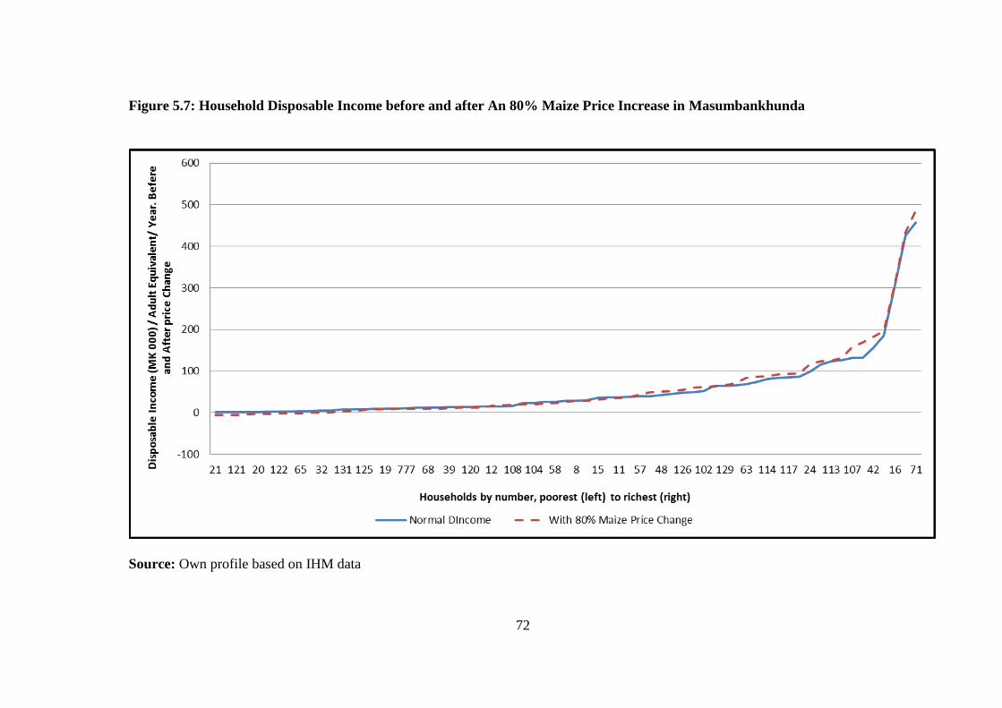
72
Figure 5.7: Household Disposable Income before and after An 80% Maize Price Increase in Masumbankhunda
Source: Own profile based on IHM data

73
The study conducted simulation where two lines were used to ascertain if the
household is losing or gaining income as a result of a price shock. The two lines used
were a solid line which represented household disposable income in the baseline. The
other line was dotted which shows household disposable income after price shock. In
Mtimaukanena, Figure 5.6, of 45 households who were above the poverty line before
the shock was introduced against 53 total households one (2 percent) fell below the
poverty line after the shock. In additional 19 households of 45 (42 percent) above
poverty line indicated a decrease in disposable income. Taking all households
together 51 percent of households had a fall in income. These are households
presented with solid line falling above the dotted line.
In Masumbankhunda 67 (100 percent) households who were above the
poverty line 10 (15 percent) fell below the poverty line. This means that after the price
shock only 85 percent had income above the poverty line. In additional 37 (55
percent) households indicated a decrease in disposable income, less than 50 percent of
village population indicated increase disposable income. The study noted that in
Figure 5.7 to the left of the figure (poorest households) had a decrease in their
incomes as shown from the solid line being above the dotted line indicating that these
are net buyer households. Net buyer households had a fall in disposable income per
adult equivalent, hence a welfare loss. These results highlight the results in Table 5.8
in section 5.21 that there were more net buyers than sellers in the study area. This
implies that many households will experience a fall in income when prices of maize
increase. From these results it can be concluded that maize price increase is sufficient
but not necessary phenomena to improve rural household income or welfare.
The study also conducted a sensitivity analysis where the effect of 95 percent
maize price increase was analysed. This is the percentage increase calculated based on

74
the study area price data. However the results were similar to results in Figure 5.6 and
5.7 that indicate that maize price increase has effect on household disposable income.
Below is Figure 5.8 and5.9 with results of changes in household disposable income
with 95 percent price increase.

75
Figure 5.8: Household disposable income before and after an 95% maize price increase in Mtimaukanena
Source: Own Profile based on IHM data
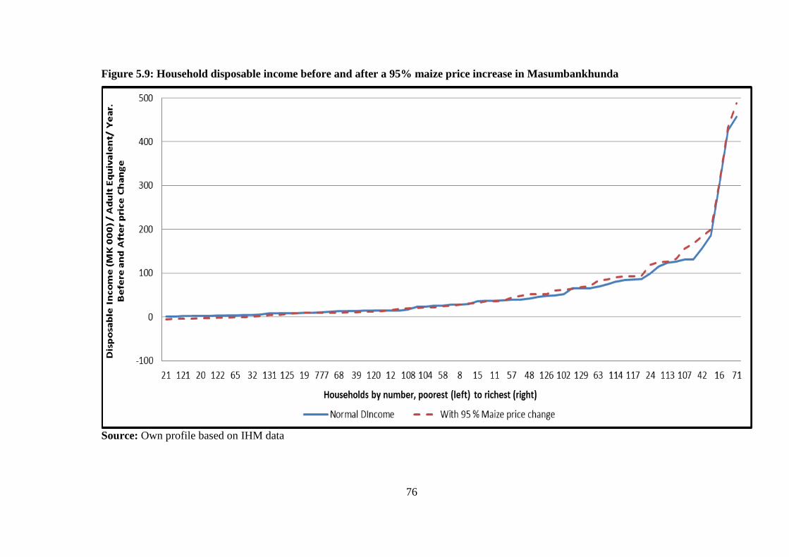
76
Figure 5.9: Household disposable income before and after a 95% maize price increase in Masumbankhunda
Source: Own profile based on IHM data

77
Both Figure 5.8 and 5.9 indicate that the net buyers (poorest households) to
the left of the figures experienced a fall in disposable income. The better off had solid
line above the dotted line indicating that they are net sellers of maize. Therefore the
effect remained the same as discussed in Figures 5.6 and 5.7 above. The only
difference is the magnitude.
Simulated Change in Disposable Income by Quintile
In Table 5.9 below, the households were grouped into five income categories
as described in section 5.2.1 of this Chapter. This table gives the summary of findings
from Figure 5.6 and 5.7 above. And also present the percentage share of income from
each income quintile to total village income by disposable income.
Table 5.9: Simulated Changes in Disposable Income, Mtimaukanena
Income
quintile
Mean DI (000) MK Simulation Total
Mean
Baseline
Mean
Simulation Change in DI
Percent
Change
(%)
Share N
Quintile1 -1263.39 -4097.049 -2833.66 -224.29 -0.79 11
Quintile2 8976.85 6185.53 -2791.32 -31.09 5.63 11
Quintile3 19,000.58 19600.99 600.41 3.16 11.92 11
Quintile4 42,048.87 45,802.65 3,753.78 8.93 23.99 10
Quintile5 103,869.3 113,210.3 9,341 8.99 59.25 10
Total 33,076 34,504 1,427.9 4.32 100 53
Source: Own computations based on IHM data
From Table 5.9 it can be seen that in Mtimaukanena in quintiles one and two,
households had a fall in disposable income. In the poorest group (quintile1), there
was an average disposable income of MK1,263.39. After simulation there was an
average decline in disposable income of MK 2,833.66. This means that 224.29
percent of disposable income on average was lost, indicating the hefty effect of the

78
shock to the poorest households. These results imply that majority households in this
quintile are net buyers.
However, it can be noted that overall, there was an gain of 4.32 percent
indicating that the few net sellers in the village were far much rich, had 59.25 percent
share of village income and may outweigh the net buyers. The highest number in
terms of increased change in income was reported in the firth category (MK 9,341).
This indicates that firth category had more net sellers than other income categories.
Table 5.10: Simulated Changes in Disposable Income, Masumbankhunda
Income
quintile
Mean DI (000) MK Simulation Total
Mean
Baseline
Mean
Simulation
Change in DI
Percent
Change
(%)
Share
N
Quintile1 3538.71 -1763.621 -5,302.3 -149.84 1.29 14
Quintile2 12227.82 10909.67 -1,318.2 -10.78 4.48 14
Quintile3 29870.16 28536.47 -1,333.7 -4.46 10.17 13
Quintile4 60044.85 67748.51 7,703.7 12.83 20.44 13
Quintile5 186821.2 201415.3 14,594.1 7.81 63.6 13
Total 56,989.58 59,673.85 2,684.26 4.7 100 67
Source: Own computations based on IHM data
Table 5.10 shows that in quintiles one, two and three, households had a fall in
disposable income. In the poorest group (quintile1), there was a decline in disposable
income of MK 5,302.33 and 149.84 percent of disposable income on average was
lost. This is consistence with Table 5.8 that all households in this category were net
maize buyers. The highest number in terms of increase in income was reported in the
firth category (MK 14,594.10). The firth category had a great share of income (63.6
percent). It can therefore be concluded that the net sellers were richest and
79
outweighed the net buyers therefore taking all households together; there was an
increment of 4.7 percent.
In order to gain an insight of the distribution of welfare gains and losses after
price shock, two measure of welfare were used. The first was disposable income
discussed in section 5.3.1 above. The second is living standard threshold (STOL)
discussed in the next section. Standard of living threshold take into account of both
food and non-food cost. Therefore, the next section discusses the simulation results on
effect of maize price shock to individual household poverty.
5.3.2 Change in Individual Household Poverty due to Maize Price Increase
The non-food costs used to set the standard of living are allocated to a
household. The household with a larger household size will have higher costs than
that with smaller number size. The non-food cost8 collected during the survey
allowed having a basis for calculating the change in poverty or impact of the shock on
poverty before and after simulations. The analysis for poverty measured by living
standards threshold (STOL) follow a similar pattern as in disposable income. The
main difference is that the analysis based on STOL shows the households that are
below and above the living standard threshold. In this thesis the other difference is
that analysis of STOL shows the impact of a change on individual household.
Figure 5.10 and 5.11 below illustrates poverty status of individual household
in the model and poverty status of individual household after model simulation, based
on STOL poverty measures. In the Figures, the dark bars and dash bars give STOL for
the households in the baseline, thus before model simulation. The dark bars indicate
the households that are falling below the standard living threshold. In the legends, DI
8 See appendix 2a

80
below STOL means the households that are below the living standard threshold and
simulation DI, is the simulation results following maize price increase.
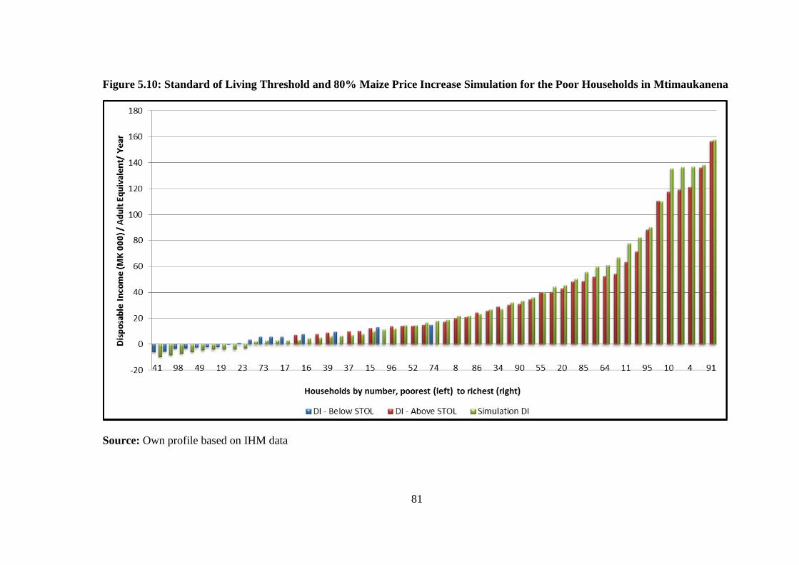
81
Figure 5.10: Standard of Living Threshold and 80% Maize Price Increase Simulation for the Poor Households in Mtimaukanena
Source: Own profile based on IHM data

82
Figure 5.10 indicates that 17 households representing 32 percent of the total
households were living below the standard of living threshold. This implies that there
was high poverty in the village even before maize price increase. After model
simulation only one household which was below STOL had a gain in income of MK
2,973 per adult equivalent. This implies that this household was among net sellers.
Therefore household can move from poverty if it is a net seller. Seven households that
were above STOL had a negative change in income after simulation. This implies that
households with a higher living standard can fall into poverty if it is a net buyer.
Further the results imply that for a given shock poorest people are getting
poorer. The households in the ‘better off’ category are benefiting more from the price
increase. These are households that are already above the STOL. The impact is mixed
in the middle category. This is in line with disposable income poverty measure that
poor households will suffer more from this shock. Below is the finding for
Masumbankhunda.

83
Figure 5.11: Standard of Living Threshold and 80% Maize Price Increase Simulation for the Poor Households in
Masumbankhunda
Source: Own profile based on IHM data

84
Figure 5.11indicates that in Masumbankhunda, 22 households representing 31
percent of households were living below the standard of living threshold. The effects
in Masumbankhunda follow a similar pattern as in Mtimaukanena, poor households
are getting poorer. There were 10 households which were above the poverty line but
an increase in maize price has pushed the households below the poverty line.
However for some households especially in middle group the change was small. It is
not surprising to note that the better off households are benefiting from maize price
increase. This is consistent with the disposable income measure of welfare and study
conceptualisation and theory used that, many rich people are surplus producers of
staple food or net sellers and tend to benefit from price increase.
These results are informative as they clearly indicate that the negative impact
of increased maize prices was felt much in the two villages. However the increase in
price of maize did not negatively affect much the middle and better off households in
the highest income group. This is because a large proportion of middle and highest
income households are net maize sellers as indicated in table 5.8. The lowest and
lower mid income group suffered most. Several reasons may account for this as noted
in the socio-economic and demographic characteristics of households by income
quintile. These include increased proportion of female heading and small cultivated
piece of land compare to middle and rich households. Results from focus group
discussion revealed that poor households were engaging in hiring out agricultural
labour especially in agricultural season which reduces own farm labour input and had
low yield due to inadequate farm inputs despite subsidy fertiliser.

85
5.5 Conclusion
In this section the study used data from IHM to analyse the effect of price
shock on household disposable income. Income was used as an indicator of poverty or
welfare. Two alternatives measures of welfare were used to establish the results,
disposable income per adult equivalent and STOL. The results indicate that the poor
are suffering. Further conclusions follow in the next Chapter. The next chapter will
summarize and conclude the thesis as well as draw some policy implications. It will
also highlight the study limitations and direction for further studies.

86
CHAPTER SIX
CONCLUSIONS
6.1 Summary of the Study
Motivated by maize price shock, this thesis modelled the distributional effect
of maize price increase on income an indicator of welfare in the rural households in
Malawi. Maize is the main staple food in Malawi. Price shock would bring a
significant effect to household welfare. The thesis used Individual Household Method
(IHM) a new approach to modelling poverty analysis that relied on primary data
collected in two sampled villages of Malawi in Dowa and Lilongwe districts, both in
the Kasungu-Lilongwe plain, central region of Malawi.
6.2. Main Findings and Conclusions
The results of the study have shown that the effect of a rise in maize on
disposable income is largely mixed. Rises in maize price worsen the welfare of a great
proportion in both villages. In Mtimaukanena 51 percent were net buyer of maize and
in Masumbankhunda 55 percent were net buyers of maize during the reference year,
hence it was observed that more than 50 percent of the villages population were
negatively affected by the shock. However at village level the effect was positive.
There was a gain in welfare of 4.32 percent in Mtimaukanena and 4.7 percent in
Masumbankhunda. This was because the highest and mid highest income households
had a great share of income which outweighed the losers. The lowest, low middle and
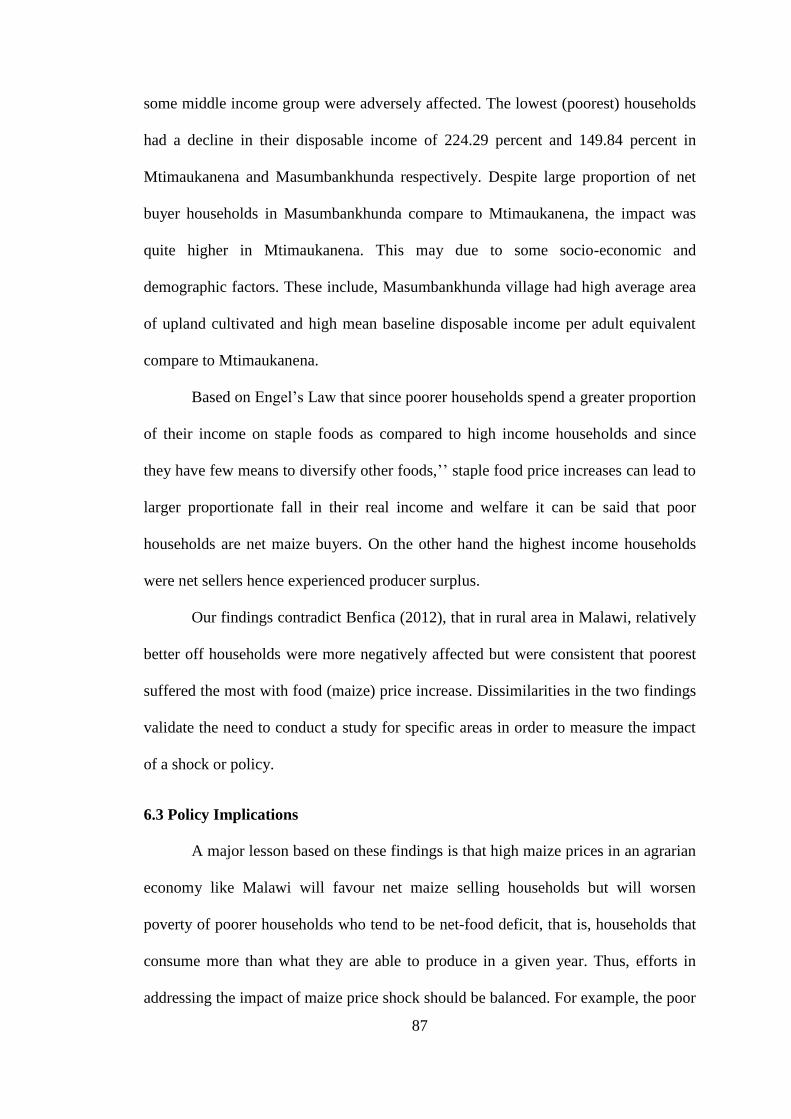
87
some middle income group were adversely affected. The lowest (poorest) households
had a decline in their disposable income of 224.29 percent and 149.84 percent in
Mtimaukanena and Masumbankhunda respectively. Despite large proportion of net
buyer households in Masumbankhunda compare to Mtimaukanena, the impact was
quite higher in Mtimaukanena. This may due to some socio-economic and
demographic factors. These include, Masumbankhunda village had high average area
of upland cultivated and high mean baseline disposable income per adult equivalent
compare to Mtimaukanena.
Based on Engel’s Law that since poorer households spend a greater proportion
of their income on staple foods as compared to high income households and since
they have few means to diversify other foods,’’ staple food price increases can lead to
larger proportionate fall in their real income and welfare it can be said that poor
households are net maize buyers. On the other hand the highest income households
were net sellers hence experienced producer surplus.
Our findings contradict Benfica (2012), that in rural area in Malawi, relatively
better off households were more negatively affected but were consistent that poorest
suffered the most with food (maize) price increase. Dissimilarities in the two findings
validate the need to conduct a study for specific areas in order to measure the impact
of a shock or policy.
6.3 Policy Implications
A major lesson based on these findings is that high maize prices in an agrarian
economy like Malawi will favour net maize selling households but will worsen
poverty of poorer households who tend to be net-food deficit, that is, households that
consume more than what they are able to produce in a given year. Thus, efforts in
addressing the impact of maize price shock should be balanced. For example, the poor
88
who have a welfare loss should be compensated to ensure equity in welfare. This can
be done by providing safety-nets to address the immediate impact of the shock on
poor households as well as enhancing increased productivity in the agricultural sector.
The results also have implications for targeting of poverty alleviation interventions
given that some household groups are affected more severely by the shock than
others.
6.4 Study Limitations and Area for Further Research
The major limitation of this study is; it focused at village level in one
livelihood plain but further studies could assess the effect employing the same
analysis in different livelihood zones especially in the southern region of Malawi,
where production of maize is known to be low and households have other major
sources of income in preference to farming. Further studies could also be conducted at
district, or national level to garner a more informative picture thereby better inform
policy analysis and programming of interventions aimed at cushioning the households
from maize price shocks.

89
REFERENCES
Aksoy, A. and A. Isik-Dikmelik (2008). Are Low Food Prices Pro-Poor? Net Food
Buyers and Sellers in Low-Income Countries. World Bank Policy Research
Working Paper No. 4642.
Badolo F. (2012). Impact of Rising World Rice Prices on Poverty and Inequality in
Burkina Faso. Retrieved February 17, 2013, from:
http://www.cerdi.org/uploads/ed/2012/2012.22.pdf
Barrett, Christopher B., and Paul A. Dorosh. (1996). Farmers‚ Welfare and Changing
Food Prices: Nonparametric Evidence From Rice In Madagascar. American
Journal of Agricultural Economics, 78(3), 54-62.
Benfica, R.. (2012). Welfare and Distributional Impacts of Price Shocks in Malawi:
Non-Parametric Approach. Selected Poster prepared for presentation at the
International Association of Agricultural Economists (IAAE) Triennial
Conference, Foz do Iguaçu, Brazil.
Byerlee, D., T.S. Jayne and R. Myers (2006). Managing Food Price Risks and
Instability in a Liberalizing Market Environment: Overview and Policy
Options. Food Policy, 31(4), 275-287.
Chayanov, A. V. (1966). The Theory of Peasant Economy. Retrieved 2012,
November 12 from

90
http://www.uky.edu/~tmute2/geography_methods/readingPDFs/chayanov-
intro.pdf
Chirwa, E. W. (2004). Trade Policy and Poverty Reduction: Evidence from Malawi.
London: Overseas Development Institute.
Budd, J.W. (1993). Changing Food Prices and Rural Welfare: A Nonparametric
Examination of the Côte d'Ivoire. Economic Development and Cultural
Change, 41(3), 587-603.
Deaton, A. & Muellbauer, J. (1980). Economics and consumer behaviour.
Cambridge: Cambridge University Press.
Deaton, A. (1989). Rice Prices and income Distribution in Thailand: A Non-
Parametric Analysis. Economic Journal, 99(395), 1–37.
Deaton, A. & Laroque, G. (1992). On the Behavior of Commodity Prices. Review of
Economics Studies, 59(1), 1–23.
Deaton, A. (1997). The Analysis of Household Surveys: A Microeconometric
Approach to Development Policy. Baltimore: Johns Hopkins University Press
for the World Bank.
91
Dessus, S., Herrera, S. & De Hoyos, R. (2008). The impact of food inflation on urban
poverty and its monetary cost: some back-of-the-envelope calculations.
Agricultural Economics, 39(1), 56-64.
Dorward, A Chirwa, E and Jayne, TS (2010). The Malawi Agricultural Inputs Subsidy
Programme, 2005/6 to 2008/9. Retrieved 2013, February 2 from:
http://siteresources.worldbank.org/AFRICAEXT/Resources/258643-
1271798012256/MAIP_may_2010.pdf.
Easterly, W. & Fischer, S. (2001). Inflation and the Poor. Journal of Money, Credit
and Banking, 33(2), 160-178.
FAO ( 2008). National Policy Responses to High Food Prices. Economic and Social
Perspectives Policy Brief 1. Retrieved 2012, March 4 from
ftp://ftp.fao.org/docrep/fao/011/ak371e/ak371e00.pdf
FAO (2012). Food Price Index. Retrieved 2013, March 09 from
http://www.fao.org/worldfoodsituation/wfs-home/foodpricesindex/en/
FEWSNET (2009). Livelihood Map. Retrieved 2012, March 01 from
www.fews.net/livelihood/mw/Maps.ppt for plain map
FEWS_NET (2012). Malawi Food Security Outlook February through June 2012.
Retrieved 2013, February 12 from
http://www.fews.net/docs/Publications/Malawi_OL_2012_02.pdf.

92
Government of Malawi GOM (2006). Malawi Growth and Development Strategy:
From Poverty to Prosperity 2006 – 2011. Lilongwe, Malawi: Ministry of
Economic Planning and Development.
Grant, W., Wolfaardt, A., & Louw A. (2012). Maize value chain in the SADC region
(Technical report). Retrieved 2012, October 25 from
www.satradehub.org/.../value-chains/maize-value-chain-in-the-sadc-regi
Gravelle, H. & Rees, R. (2004). Microeconomics. London: Prentice Hall.
Gujarati, D.N. (2004). Basic Econometrics (4th ed.). New York: Mc Graw-Hill.
Hoyos, R. E. & Medvedev, D. (2008). Poverty Effects of Higher Food Prices: A
Global Perspective. Review of Development Economics,15(3), 387–402.
Ivanic, M. & Martin, W. (2008). Implications of Higher Global Food Prices for
Poverty in Low-Income Countries (Policy Research Working Paper 4594).
Washington DC: World Bank.
Karfakis, L. Tasciotti, S. DiGiuseppe & G. Bonomi, (2007). Rural Household Access
to Assets and Agrarian Institutions: A Cross Country Comparison.
(Background Paper for the World Development Report 2008). Rome: FAO
Khonje, M. (2010). Food Inflation in Malawi: Implications For The Economy
(Unpublished master’s thesis). Makerere University, Kampala, Uganda.

93
Kreps, D.M. (1990). A Course in Microeconomic Theory. Princeton, NJ: Princeton
University Press.
Malawi Vulnerability Assessment Committee (MVAC 2012). National Food Security
Forecast, April 2012 to March 2013. Retrieved 2013, March 16 from
http://www.sadc.int/fanr/aims/rvaa/Documents/Malawi/MVAC%20Annual%2
0Report%20June%202012%20_final%20030712.pdf.
Malawi Government (2013). 2011/12 Annual Agricultural Statistical Bulletin.
Lilongwe: Ministry of Agriculture and Food Security, Planning Department.
Mas-Collel, A., Whinston, M. & Green, J. R. (1995). Microeconomic Theory. New
York: Oxford University Press.
Mellor, J. W. (1978). Food price policy and income distribution in low-income
countries. Economic Development and Cultural Change, 27 (1), 1–26.
Minot, N. & Goletti, F. (2000). Rice Market Liberalization and Poverty in Viet Nam
(Research Report 114). Washington DC: International Food Policy Research
Institute.
Minot, N. (2010, January). Staple food prices in Malawi. Paper presented at the
Comesa policy seminar on Variation in staple food prices: Causes,
consequence, and policy options, Maputo, Mozambique.

94
MoAFS (2012). Final round crop estimates. Lilongwe, Malawi: Ministry of
Agriculture and Food Security.
MoAFS (2013). Food Prices. Retrieved 2013, February 23 from www.moafsmw.org.
Msukwa, L. A. H. (1994). Food Policy and Production: Towards Increased
Household Food Security. Zomba: Centre for Social Research.
National Statistical Office (2005). Malawi Second Household Survey (IHS-2) 2004 –
2005: Basic Information Document. Retrieved 2013, February 03 from
http://www.nso.malawi.net.
National Statistical Office (2005). Household Socio-economic characteristics
Integrated Household Survey 2 (1), 2004-2005. Zomba: National Statistical
Office.
National Statistical Office (2008). 2008 Population and housing: Preliminary Report.
Retrieved 2013, February 12 from: www.nso.org.
Nicholson, Walter. (2001). Microeconomic Theory: Basic Principles and Extensions.
(8th ed.). Ohio: South-Western College Pub.
Ravaillon, M. (1990). Rural welfare changes of food prices under induced wage
responses: theory and evidence from Bangladesh. Oxford Economic Papers,
42, 574-85.
95
Ravallion, M. (1998). Poverty Lines in Theory and Practice. Living Standards
Measurement Study Series. Washington, DC: World Bank.
Ravallion, M. & Datt, G. (2002). Why has economic growth been more pro-poor in
some states of India than others? Journal of Development Economics 68, 381-
400.
Rios, A. R., Masters, W.A. & Shively, G.E. (2008). Agricultural Prices and Income
Distribution among Farmers: A whole-Household, Multi-Country, Multi-Year
Analysis. Mimeo: Purdue University.
Seaman J., and Petty C., (2010).The Individual Household Method (IHM): An
overview. Evidence for Development. Retrieved 2012, December 21 from
http://www.evidencefordevelopment.com.
Sen, A. (1980). Levels of poverty: policy and change: a background study for World
Development Report (Staff Working Paper 401). Washington D.C.: World
Bank.
Sen, A. (1981). Poverty and famines: an essay on entitlement and deprivation. New
York: Oxford University Press Inc.
Seshan, G. & Umali-Deininger, D. (2007). Agriculture and Import Liberalization and
Household Welfare in Sri Lanka. Retrieved 2012, October 12 from
96
http://siteresources.worldbank.org/INTPSIA/Resources/490023-
1120841262639/PSIA_SriLanka_Agriculture_Import_Liberalization.pdf
Singh, I., Squire, L. & Strauss, J. (eds), (1986). Agricultural Household Models:
Extensions, Applications, and Policy. Baltimore, MD: Johns Hopkins
University Press for the World Bank.
Taylor, J. E. (2003). Agricultural Household Models: Genesis, Evolution, and
Extensions. Review of Economics of the Household, 1(1), 12-25
Ulimwengu, J. & Ramadan, R.. (2009). How does food price increase affect Ugandan
households? An augmented multimarket approach (Discussion Paper 00884).
Washington, DC: International Food Policy Research Institute.
UN FAO (2012). FAO Food Price Index March. Retrieved 2013, November 12 from
http://www.fao.org/worldfoodsituation/wfs-home/foodpricesindex/en/m
Varian, H. R. (1992). Microeconomic Analysis (3rd ed.). London: Norton &
Company.
Varian, H. R. (2005). Intermediate Microeconomics: A Modern Approach (7th
ed.).
London: Norton & Company.

97
Wodon, Q. &. Zaman, H. (2008). Rising food prices in Sub-Saharan Africa: Poverty
impact and policy responses (Policy Research Working Paper 4738).
Washington, DC. : World Bank.
World Bank (2003). Malawi Country Economic Memorandum: Policies for
Accelerating Growth. Washington: World Bank.
World Bank (2008). Rising food prices: policy options and World Bank Response.
(Paper prepared as background to the Meetings of the Development
Committee). Retrieved 2012, November 01, from
http://siteresources.worldbank.org/NEWS/Resources/risingfoodprices_backilo
gramroundnote_apr08.pdf.
World Bank (2009). Malawi Country Economic Memorandum – Seizing
Opportunities for Growth Through Regional Integration and Trade, 1.
Washington, D.C.: World Bank.
World Bank (2011, February). Food Price Watch. Retrieved March 6, 2013 from
http://www.worldbank.org/foodcrisis/food_price_watch_report_feb2011.html.
World Bank (2012). Poverty Manual (JH Revision of 2005). Retrieved 2013, March
01 from http://siteresources.worldbank.org/PGLP/Resources/ch5.pdf.

98
APPENDICES
Appendix 1: Average Monthly Maize Price in Malawi Kwacha per Kilogram
Month 2010/2011 2011/2012 2012/2013
May 30.58 23.75 39.65
June 29.80 24.19 48.04
July 29.70 29.16 54.12
August 30.60 28.21 55.95
September 30.60 30.06 56.18
October 29.57 32.75 58.59
November 30.13 36.14 63.21
December 30.48 40.14 72.95
January 30.80 56.23 89.44
February 31.17 52.07 111.14
March 32.99 47.79
April 28.66 42.21
Average 30.42 36.89 59.02
Source: MoAFS, 2013
Month 2010/2011 2011/2012 2012/2013
May 30 52 60
June 30 52 60
July 30 52 60
August 30 52 60
September 30 52 60
October 30 52 60
November 30 60 60
December 30 60 60
January 30 60 60
February 30 60 60
March 52 60
April 52 60
Average 34 56 60
Source: Administrative data ADMARC

99
Appendix 2a: Items used in establishing STOL, Masumbankhunda
ITEM ANNUAL
COST (MK)
Household
Salt 6,000
soap 24,000
Lighting 2,400
Individual
Stationary primary 1,400
School uniform-female
School uniform-Male
2,000
1,000
Clothes male child
Clothes female child
Clothes adult male
Clothes adult female
3,000
6,000
5,000
7,000
Lotion
Children female
Children Male
Adult male
Adult female
6,000
6,000
3,600
7,200
Source: IHM study data

100
Appendix 2b: IHM Interview Form
Individual Household Economy:
AGRICULTURAL YEAR ..........................
Date: Household #
Place:
Interviewer: Interviewee:
Have you (i) explained the purpose of the interview (ii) covered confidentiality and (iii) explained that participation is voluntary?
Y/N
Has the interviewee given their consent? Y/N
1. Name of current household head: Record the name they would use for ‘official’ purposes

101
2. Details of all household members: Include everyone who eats and sleeps here; also include ‘part time’ residents ie family members
who work away for part of the year but contribute to household income.
Name
For children of school age. Is child in
school?
Indicate Primary or Secondary. ( Do
not include household members who
have left school.)
Sex Age Full time
or p/time
If part time, approx how
many weeks present per
year?
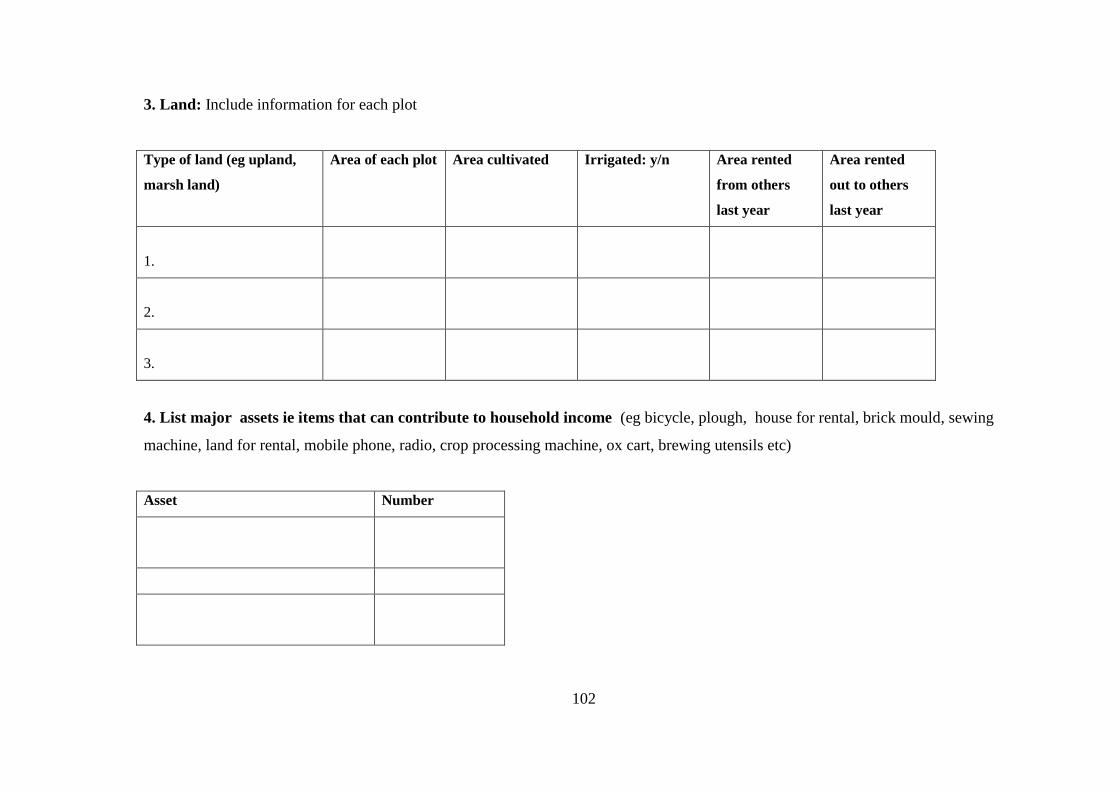
102
3. Land: Include information for each plot
Type of land (eg upland,
marsh land)
Area of each plot Area cultivated Irrigated: y/n Area rented
from others
last year
Area rented
out to others
last year
1.
2.
3.
4. List major assets ie items that can contribute to household income (eg bicycle, plough, house for rental, brick mould, sewing
machine, land for rental, mobile phone, radio, crop processing machine, ox cart, brewing utensils etc)
Asset Number
103
Livestock. List livestock held by the household during the study period
Animal Number

104
5. Production : With the interviewee, make a sketch of their plot/s and indicate the size of plot/s, and list all the crops grown on that land
in the last full agricultural year . Use the back of this sheet and indicate Season 1/ Season 2 where relevant. Then fill in the following
table, indicating total production, amount sold, other uses and amount consumed by the household. Do not attempt to convert local
measures to kg during the interview. Check if ‘sacks’ are 90kg or 50kg.
NB INCLUDE GREEN CROPS (eg GREEN MAIZE-also referred to as ‘fresh maize’) as separate items
Crop
Note if improved plant
material is used
Total
Production
local
measure.
Total
Producti
on (Kg)
Amount
sold
Sale
price/unit
Month sold Other uses eg given
away, saved for seeds
etc
Amount consumed by
household(Kg)
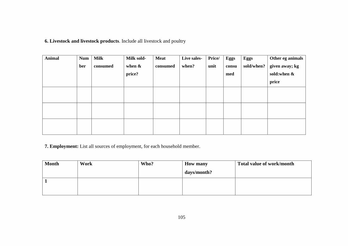
105
6. Livestock and livestock products. Include all livestock and poultry
Animal Num
ber
Milk
consumed
Milk sold-
when &
price?
Meat
consumed
Live sales-
when?
Price/
unit
Eggs
consu
med
Eggs
sold/when?
Other eg animals
given away; kg
sold:when &
price
7. Employment: List all sources of employment, for each household member.
Month Work Who? How many
days/month?
Total value of work/month
1
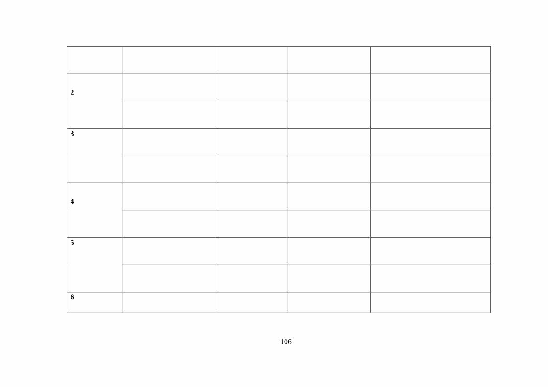
106
2
3
4
5
6

107
7
8
9
10
11
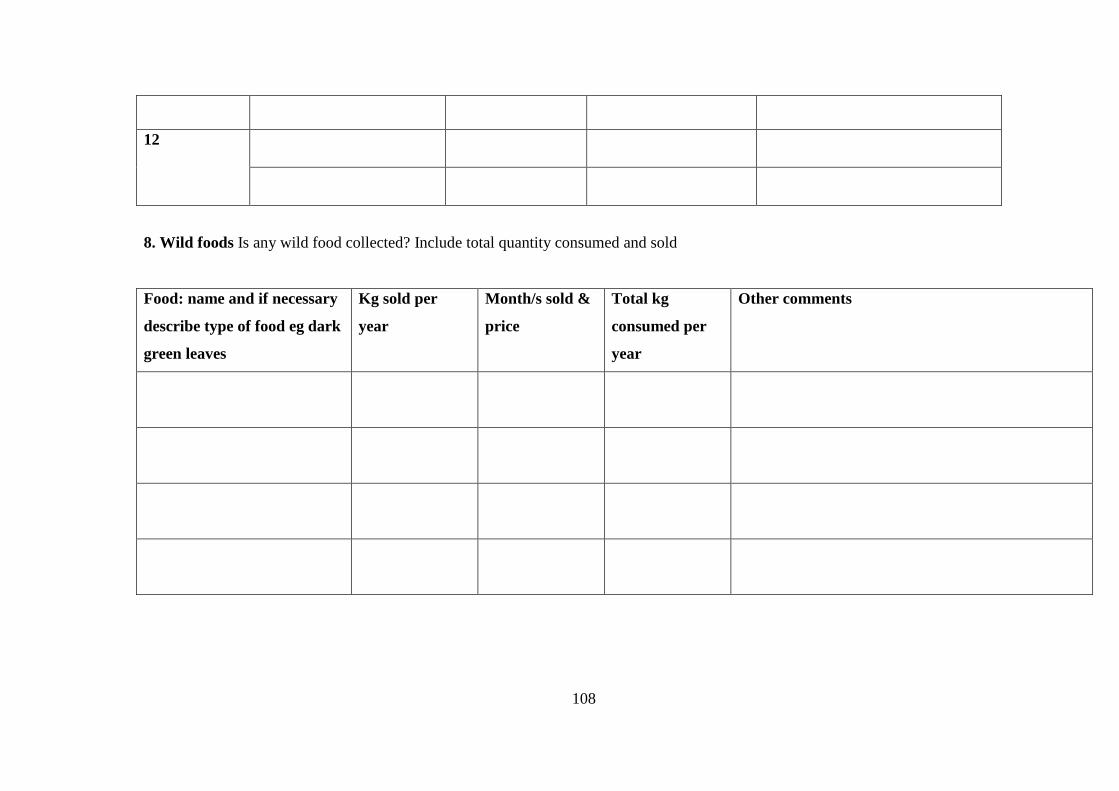
108
12
8. Wild foods Is any wild food collected? Include total quantity consumed and sold
Food: name and if necessary
describe type of food eg dark
green leaves
Kg sold per
year
Month/s sold &
price
Total kg
consumed per
year
Other comments

109
9. Transfers: Include all sources including relief, support from relatives who are not part of the household, neighbours etc
10. Other food transfers: check if any food is gained by children or others eg gleaning after the harvest; begging etc
Food Total kg consumed
per year
Other comments – eg when the food is given to the family
Source of
assistance: NGO,
neighbour,
church, relative,
government relief
Type of assistance. If
food, record food type
eg maize, cassava etc
Quantity:
if food ,
total kg.
If cash,
total per
year
If food, quantity
sold
If food quantity
kept for own
consumption
Other information eg
when assistance was
received
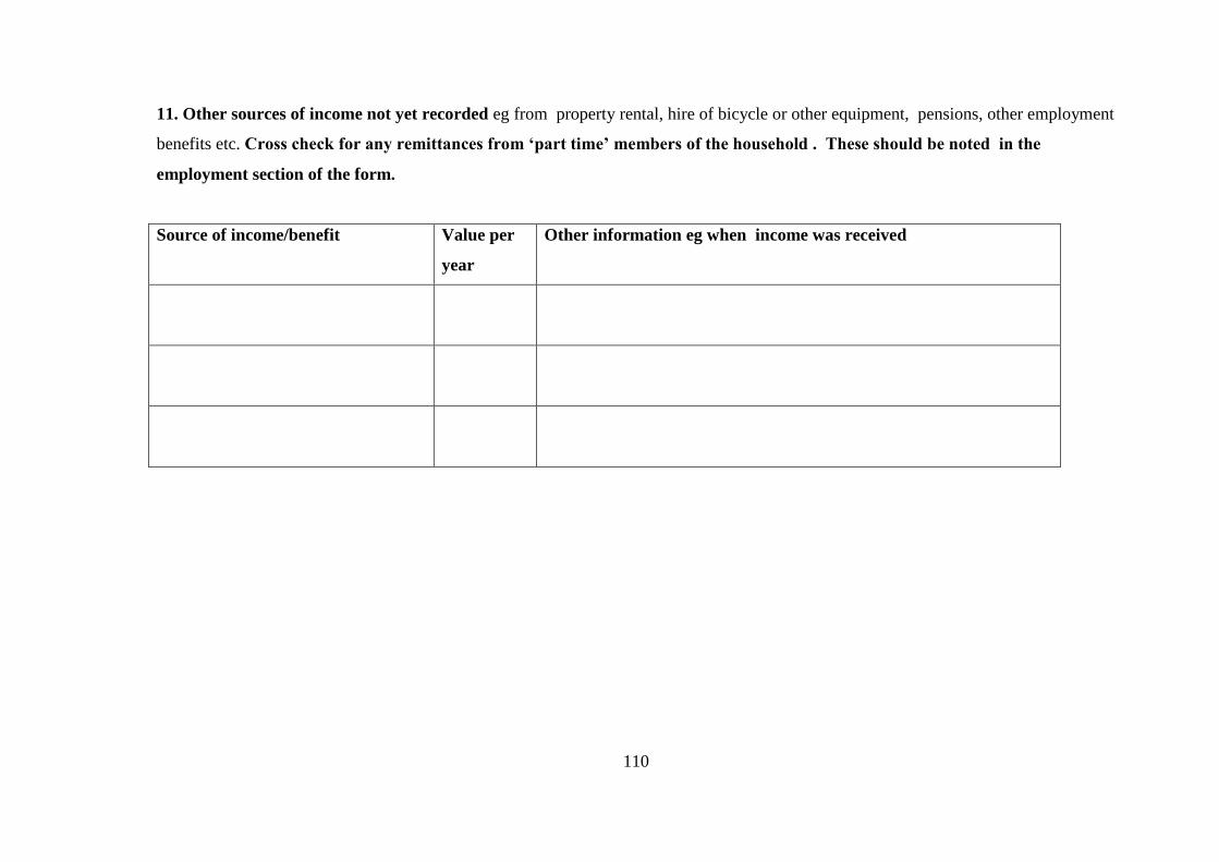
110
11. Other sources of income not yet recorded eg from property rental, hire of bicycle or other equipment, pensions, other employment
benefits etc. Cross check for any remittances from ‘part time’ members of the household . These should be noted in the
employment section of the form.
Source of income/benefit Value per
year
Other information eg when income was received

111
12. Credit and loans
Did you need credit during the survey period?
If yes, did you get credit?
Source of credit
Purpose of loan Value of loan Repayment per
month
Total repayment
13. Are any adults in the household unable to work due to disability or old age? Who?
14. Did any household member die during the study period (use appropriate term eg ‘pass away.’) Who? In which month did
this happen?
Do you have any questions or comments?

112
Appendix 3: Map of Malawi showing Livelihood Zones and their activities
Source: FEWSNET (2009)


![Chirwa consolidated judgment - SAFLII · SKWEYIYA J 5 [11] Ms Chirwa refused to participate in the 22 November 2002 enquiry on the grounds that she objected to Mr Smith being “the](https://img.dokumen.tips/doc/110x75/5b92a0c109d3f23a718c308d/chirwa-consolidated-judgment-skweyiya-j-5-11-ms-chirwa-refused-to-participate.jpg)