Turk J Elec Eng & Comp Sci

(2016) 24: 4804 – 4823

c⃝ TUBITAK

doi:10.3906/elk-1404-409

Turkish Journal of Electrical Engineering & Computer Sciences

http :// journa l s . tub i tak .gov . t r/e lektr ik/

Research Article

Modeling, control, and power management for a grid-integrated photo voltaic,

fuel cell, and wind hybrid system

Ezhilarasan GANESAN∗, Subhranhsu Sekhar DASH, Chinmaya SAMANTADepartment of Electrical and Electronics Engineering, SRM University, Kancheepuram, India

Received: 15.04.2014 • Accepted/Published Online: 17.09.2015 • Final Version: 06.12.2016

Abstract: Power management in a grid-integrated power system consisting of distributed renewable energy sources is

necessitated by ever-increasing energy consumption, the high cost of production, the limited resource of fossil fuel, and

the worsening global environment. Wind and solar power generation are two of the most promising renewable power

generation technologies. The growth of wind and photovoltaic (PV) power generation systems has exceeded the most

optimistic levels of expectations. Fuel cells (FCs) also have great potential to be green power sources of the future

because of the many merits they have, such as high efficiency and zero or low emission of pollutant gases. In this paper

the modeling, control, and analysis of grid-connected PV power, a proton exchange membrane fuel cell (PEMFC), and

a wind energy system (WES) connected through a common DC bus linked to an AC grid is discussed. In coordination

with the PEMFC, the hybrid system’s output power becomes controllable so that full utilization of PV and wind power

takes place based on its availability, and the DC bus voltage is maintained constant even at varying load conditions for

the desired power sharing between the distributed generation (DG) sources, load, and the AC grid. The hybrid system

is controlled through a combination of two proposed control modes, namely the DG control mode and grid control

mode. The coordination of the power controller, voltage source converter controller, and load controller is such that

the transition between the two control modes is done as smoothly as possible. Thus, the total DG power will be a

combination of PV power, WES power, and power produced by the PEMFC. Any additional power if required up to the

maximum loading will be supplied by grid. If the load exceeds its maximum value, then the load controller will carry out

load shedding. The composite system is available for safe operation in on-grid as well as off-grid mode satisfying voltage

and power balance constraints. Different modes of operation have been demonstrated to verify and validate the desired

power management among the DG sources, load, and the grid. MATLAB/Simulink software was used for simulating the

composite model.

Key words: Distributed generation, grid-controlled mode, distributed generation control mode, wind energy system,

power management, fuel cell

1. Introduction

A major percentage of all electrical power is produced through conventional energy sources alone; hence, the

reserves of coal and fossil fuels are diminishing at a fast rate. Therefore, due to these limitations, a new

method has to be found to balance supply and demand without resorting to conventional generation, as stated

in [1]. Initially, alternate sources of energy like solar and wind power sources were installed with the primitive

equipment available, which resulted only in generation of additional energy without proper management of

∗Correspondence: ezhil.power@gmail.com

4804

GANESAN et al./Turk J Elec Eng & Comp Sci

generated power. Over recent years several research and investment programs have been carried out with

hybrid power systems, which recommend an optimal design model for hybrid solar–wind systems [2]. Recently,

electronic power converters and their identified usage for power systems have brought about many changes,

like the concept of distributed generation using hybrid power generation. The importance of hybrid systems

consisting of renewable energy (RE) sources has increased significantly as they appear to be an effective solution

for clean and distributed energy production. This consists of renewable energy sources such as photovoltaic

(PV) energy, wind generators, and fuel cells (FCs) along with the necessary power converters.

At present, distributed generation is assuming increased importance because of its several distinctive ad-

vantages, such as simple configuration, multiple sources, high reliability, absence of fuel costs, low maintenance,

and the fact it has absolutely no pollutants and hence is ecofriendly.

Many alternative energy sources including wind, PV, FCs, diesel systems, gas turbines, and microturbines

can be used to build hybrid energy systems. Nevertheless, the major renewable energy sources used and reported

are wind and PV power, as stated in [3]. However, the disadvantage of PV generation and wind energy systems

(WESs) is that they are characteristically unstable, being heavily dependent on weather conditions. Stand-

alone wind and PV energy systems normally require energy storage devices. The storage device can be an

electrochemical battery, ultracapacitor, magnetic energy storage, and so on.

In order to overcome the inherent drawbacks discussed above, distributed generation (DG) sources such

as PV and WESs should be combined with a proton exchange membrane fuel cell (PEMFC) to form a hybrid

system. By changing the FC output power, the hybrid source output becomes controllable and can be maintained

at a certain reference level. However, a PEMFC in turn works only at high efficiency within a specific power

range. This proposed hybrid system can be linked to the main grid or can work independently, and when in

grid-connected mode the hybrid source is connected to the main grid at the point of common coupling (PCC)

to deliver power to the load. Whenever the demand from the load changes, the power supplied by the main grid

and hybrid system must be properly managed. The power delivered from the main grid and the PV array, as

well as the PEMFC, must be coordinated to meet load demand. The hybrid generation thus can be controlled in

2 control modes: grid control mode (GCM) and distributed generation control mode (DGCM), as stated in [4].

In GCM mode, variations of load demand are compensated by the main grid because the hybrid source output is

regulated by the reference power. The proposed operating strategy is to coordinate the two control modes and

determine the reference values of the DGCM mode so that all constraints are satisfied. This operating strategy

will minimize the number of operating mode changes, improve the performance of the system operation, and

enhance system stability.

2. Working methodology of a grid-integrated hybrid system

This paper presents modeling and control strategies for power and load management of a grid-integrated hybrid

system consisting of a PV array, a PEMFC, and a WES connected through a common DC link to an AC grid

as stated in [5].

The coordination of the power controller, voltage source converter (VSC) controller, and load controller

is proposed to make the transition between the two modes as smooth as possible. The load is connected between

the DG sources and grid. With the varying load conditions, the DG output power (Pms) and grid power (Pgrid)

must be properly adjusted and coordinated so as to match the load (Pload), while fully utilizing the PV power

and WES to keep the DC bus voltage constant.

The grid-integrated hybrid system mainly works in 2 modes of operation: DGCM and GCM. As stated

4805

GANESAN et al./Turk J Elec Eng & Comp Sci

earlier, the power controller referred to in [6] coordinates the automatic change-over between these two modes

in coordination with the load controller and the inverter controller.

The system operates in DGCM when the load is less than a certain threshold (P thload) value. The output

power of the DGs is maintained at a certain reference level (Pmsref ) based on PV power availability by varying

the FC power with proper coordination [7]. When the power drawn by the load is greater than or equal to

the threshold value, but less than the maximum load (P loadmax), the hybrid system will be in GCM. FCs will

deliver fixed power operating at the lowest level (Pfclow).

In order to achieve a reliable DG setup with reduced grid dependency, the various modules of the DG

were mathematically modeled and integrated as follows: modeling of wind turbine, drive train, maximum power

point tracker (MPPT), pitch angle controller, permanent-magnetic synchronous generator (PMSG), DC/DC

converter, and the power controllers. After the modeling, the integration of a PV-FC-wind hybrid system to

the grid was done followed by the implementation of controlled mode (auto) and noncontrolled (manual) mode

of operation. Thus, the full utilization of PV and wind power was possible by maintaining a constant DC bus

voltage to achieve the desired power management between DG sources, load, and grid under all load conditions.

In the case of the power being unmanageable, local power shedding is used.

3. Modules of the grid-integrated hybrid system

The grid-integrated hybrid system, as shown in Figure 1, consists of 3 nonconventional energy sources, namely a

solar photovoltaic arrangement with a DC-DC boost converter with a perturb and observe MPPT algorithm, a

proton exchange membrane-based fuel cell with DC boost converter, and a wind energy system with its output

suitably rectified and stepped up in order to match the voltage of the common DC bus of the DG system. Thus,

Ppv , Pwind , and Pfc are obtained at the same DC level.

In order to connect DG sources to the load and the grid, the output from the DG sources is given to a

DC bus, which is further connected to a DC to 3 phase inverter VSC, from where the power Pms is fed to a

3-phase transformer and hence to the load and grid. The power fed to the grid is marked as Pgrid and that

to that of the load is marked P load . In the next section the details of the modeling of the above-mentioned

modules of the grid-integrated hybrid power system are discussed.

3.1. Modeling of photovoltaic arrays

The mathematical equations that describe the voltage-current (V-I) characteristic of the ideal photovoltaic cell

as referred to in [8] are:

I = Ipvcell − Id and Id = Iocell[exp(qV/akT )− 1], (1)

where Ipvcell is the current generated by the incident light, which is directly proportional to the solar irradiation;

Id is the Shockley diode equation; I0cell is the reverse saturation or leakage current of the diode; q is the electron

charge (1.60217646 × 10−19 C); k is the Boltzmann constant (1.3806503 × 10−23 J/K); K is the working

temperature of the p-n junction; and a is the diode ideality factor as referred to in [9].

I = Ipv − Io[exp[(V +RsI)/(aVt)]− 1], (2)

where Ipv and I0 are the photovoltaic and saturation currents of the array and V t = (NskT)/q is the thermal

voltage of the array with Ns cells in series. Rs and Rp are the equivalent series and parallel resistance of the

4806

GANESAN et al./Turk J Elec Eng & Comp Sci

Figure 1. Overall arrangement of grid-integrated hybrid power generation.

array as referred to in [10].

Ipv = (Ipvn +KI∆T )× (G/Gn), (3)

where Ipvn is the light-generated current at the nominal condition (usually 25 ◦C and 1000 W/m2), ∆T = T

– Tn (T and Tn are the actual and nominal temperatures K), G [W/m2 ] and Gn [W/m2 ] are the operating

and nominal irradiation, and KI is the current/temperature coefficient in A/K. The diode saturation current

I0 depends on temperature, as given by;

I0 = (Iscn +KI∆T )/[exp{Vocn +KV ∆T )/(aVt)} − 1], (4)

where Iscn is the nominal short-circuit current, Vocn is the nominal open-circuit voltage, and KV is the

voltage/temperature coefficient in V/K. If the photovoltaic array is composed of Nser series and Npar parallel

modules, then

I = Ipv +Npar − IoNpar[exp{{V +Rs(Nser/Npar)I}∆T )/(aVtNser)} − 1]. (5)

The PV array maximum power output is given by

PMPP = VMPP × IMPP . (6)

4807

GANESAN et al./Turk J Elec Eng & Comp Sci

3.2. Maximum power point tracker control

The role of the MPPT in PV systems is to automatically track the voltage VMPP or current IMPP at which

a PV array should operate to obtain the maximum power output PMPP under a given operating temperature

and irradiance. Most MPPT techniques respond to changes in both irradiance and temperature. In the present

work, the incremental conductance (INC) method is used, in which the problem of tracking peak power under

fast varying atmospheric condition is resolved. The INC method, as referred to in [11], is based on the fact that

the slope of the PV array power is zero at the MPP, positive on the left of the MPP, and negative on the right,

as shown in Figure 2.

Figure 2. Incremental conductance algorithm P-V/P-I characteristic.

Therefore, ∆I/∆V = –I/V at the MPP, ∆I/∆V > –I/V on the left of the MPP, and ∆I/∆V < –I/V

on the right of the MPP. The MPP can thus be tracked by comparing the instantaneous conductance (I/V)

with the incremental conductance (∆I/∆V) as stated in [12].

3.3. Modelling of the fuel cell

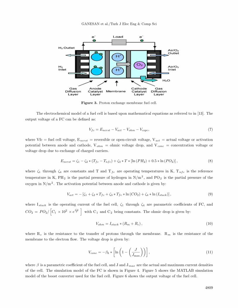
The PEMFC, as shown in Figure 3, is a nonlinear, multiple-input and multiple-output, strongly coupled, and

large-delay dynamic system that converts chemical potential into electric power. It converts the chemical energy

of a fuel.

4808

GANESAN et al./Turk J Elec Eng & Comp Sci

Figure 3. Proton exchange membrane fuel cell.

The electrochemical model of a fuel cell is based upon mathematical equations as referred to in [13]. The

output voltage of a FC can be defined as:

Vfc = Enerst − Vact − Vohm − Vcopc, (7)

where Vfc = fuel cell voltage, Enerst = reversible or open-circuit voltage, Vact = actual voltage or activation

potential between anode and cathode, Vohm = ohmic voltage drop, and Vconc = concentration voltage or

voltage drop due to exchange of charged carriers.

Enerst = ζ1 − ζ2 ∗ (Tfc − Tnfc) + ζ3 ∗ T ∗ [ln (PH2) + 0.5 ∗ ln (PO2)] , (8)

where ζ1 through ζ4 are constants and T and Tfc are operating temperatures in K, Tnfc is the reference

temperature in K, PH2 is the partial pressure of hydrogen in N/m2 , and PO2 is the partial pressure of the

oxygen in N/m2 . The activation potential between anode and cathode is given by:

Vact = − [ζ1 + ζ2 ∗ Tfc + ζ3 ∗ Tfc ∗ ln (CO2) + ζ4 ∗ ln (Istack)] , (9)

where Istack is the operating current of the fuel cell, ζ1 through ζ4 are parametric coefficients of FC, and

CO2 = PO2/[C1 × 102 × e

C2T

]with C1 and C2 being constants. The ohmic drop is given by:

Vohm = Istack ∗ (Rm +Rc) , (10)

where Rc is the resistance to the transfer of protons through the membrane. Rm is the resistance of the

membrane to the electron flow. The voltage drop is given by:

Vconc = −βk ∗[ln

(1−

(J

Jmax

))], (11)

where β is a parametric coefficient of the fuel cell, and J and Jmax are the actual and maximum current densities

of the cell. The simulation model of the FC is shown in Figure 4. Figure 5 shows the MATLAB simulation

model of the boost converter used for the fuel cell. Figure 6 shows the output voltage of the fuel cell.

4809

GANESAN et al./Turk J Elec Eng & Comp Sci

Figure 4. MATLAB simulation model of fuel cell.

Figure 5. MATLAB simulation model of boost converter used for fuel cell.

3.4. Wind energy system mathematical model and simulation

The WES as shown in Figure 7 mainly consists of a variable-speed wind turbine with a drive train (to drive

the rotor shaft), pitch angle controller, PMSG, rectifier, MPPT, DC/DC converter, and DC/AC converter, as

4810

GANESAN et al./Turk J Elec Eng & Comp Sci

Figure 6. Output voltage of a fuel cell.

referred to in [14]. The pitch angle controller takes care of the pitch of the WES such that in the case of high

wind speed or low wind speed the pitch can be adjusted as referred to in [15] to operate the wind turbine at

its optimum level. A permanent magnet synchronous generator is preferred because of its simple construction

and low maintenance. The mathematical model of the WES was derived by removing the wind energy system

from the grid-integrated hybrid system. Thus, as per the model, the WES supplies the grid, and hence the

load, directly. This is done in order to study the individual behavior of the WES so that when it is integrated

into the hybrid system the control parameters can be easily set and an accurate control can be achieved. The

output power of the turbine was referred to in [16] and is given by the following equations.

Figure 7. Schematic of a wind energy system.

Pm = Cp × (ωω )3

(12)

Tt =Pm

ωsh(13)

4811

GANESAN et al./Turk J Elec Eng & Comp Sci

λ =

(ωsh

ωω

)∗ λnom (14)

Cp = C1 +

[C2

λ− C3∗ β − C4

]∗ exp

(−C5

λ

)+ C6 ∗ λ (15)

1

λi=

1

[λ+ 0.08 ∗ β]− 0.0.35[

(β)3+ 1] (16)

Cpnom = Cpmax (17)

λinom =

(1

1λnom

− 0.035

)(18)

Knom = −

(C2 ∗ C5

λinom− C4 ∗ C5 − C2

)∗ exp

(−C5

λinom

)(λnom)

2 (19)

C1 =Cpmax((

C2

λinom− C4

)∗ exp

(−C5

λinom

)+Knom ∗ λnom

) (20)

C6 = Knom ∗ C1 (21)

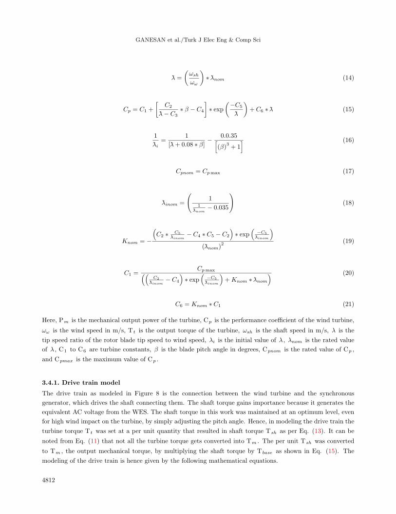
Here, Pm is the mechanical output power of the turbine, Cp is the performance coefficient of the wind turbine,

ωω is the wind speed in m/s, T t is the output torque of the turbine, ωsh is the shaft speed in m/s, λ is the

tip speed ratio of the rotor blade tip speed to wind speed, λi is the initial value of λ , λnom is the rated value

of λ , C1 to C6 are turbine constants, β is the blade pitch angle in degrees, Cpnom is the rated value of Cp ,

and Cpmax is the maximum value of Cp .

3.4.1. Drive train model

The drive train as modeled in Figure 8 is the connection between the wind turbine and the synchronous

generator, which drives the shaft connecting them. The shaft torque gains importance because it generates the

equivalent AC voltage from the WES. The shaft torque in this work was maintained at an optimum level, even

for high wind impact on the turbine, by simply adjusting the pitch angle. Hence, in modeling the drive train the

turbine torque T t was set at a per unit quantity that resulted in shaft torque Tsh as per Eq. (13). It can be

noted from Eq. (11) that not all the turbine torque gets converted into Tm . The per unit Tsh was converted

to Tm , the output mechanical torque, by multiplying the shaft torque by Tbase as shown in Eq. (15). The

modeling of the drive train is hence given by the following mathematical equations.

4812

GANESAN et al./Turk J Elec Eng & Comp Sci

Figure 8. MATLAB model of the drive train.

Tt − Tsh = 2 ∗Ht ∗(dωt

dt

)(22)

(ωt − ωr)

ωebase=

[d (θsta)

dt

](23)

Tsh = [θsta ∗Kss +Kd ∗ (ωt−ωr)] (24)

Tbase =Pnom

ωebase(25)

Tm = Tbase + Tsh (26)

Here, H t is the inertia constant of the turbine, ωt is the angular speed of the wind turbine, ωr is the

rotor speed of generator, θsta is the shaft twist angle, Kss is the shaft stiffness coefficient, Kd is the damping

coefficient, ωebase is the electrical base speed, Pnom is the nominal power of WES, and Tbase is the base torque

of the wind turbine. The above parameters are depicted in Figure 9.

4813

GANESAN et al./Turk J Elec Eng & Comp Sci

Figure 9. Various output parameters of wind energy system.

4. Permanent magnet synchronous generator modeling

The permanent magnet synchronous generator is where the excitation field is provided by a permanent magnet

instead of a coil. Synchronous generators are the main source of commercial electrical energy. They are

commonly used to convert the mechanical power output of wind turbines into electrical power for the grid.

A set of 3 conductors make up the armature winding. The phases are wound such that they are 120◦

apart spatially on the stator, providing for a uniform force or torque on the generator rotor. The uniformity

of the torque arises because the magnetic fields resulting from the induced currents in the 3 conductors of the

armature winding combine spatially in such a way as to resemble the magnetic field of a single rotating magnet.

This stator magnetic field or “stator field” appears as a steady rotating field and spins at the same frequency

as the rotor when the rotor contains a single dipole magnetic field. The two fields move in “synchronicity” and

maintain a fixed position relative to each other as they spin.

The advantage of using permanent magnet generators in this work is that they do not require a DC

supply for the excitation circuit, nor do they have slip rings and contact brushes, and hence the maintenance is

simple. The drawback of the PMSG is that the flux density of high-performance permanent magnets is limited.

The air gap flux is also not controllable, so the voltage of the machine cannot be easily regulated. Hence, here

in this modeling all the above factors are considered and suitably modeled.

The modeling of PMSG was referred to in [17] and is carried out using the following mathematical

4814

GANESAN et al./Turk J Elec Eng & Comp Sci

equations. (dIddt

)=

(Vd

Ld

)+ ωe ∗ Iq ∗

(Lq

Ld

)− Id ∗

(R

Ld

)(27)

(dIqdt

)=

(Vq

Lq

)− ωe ∗ Id ∗

(Ld

Lq

)− ωe ∗

(λo

Lq

)− Iq ∗

(R

Lq

)(28)

Te =

(3

2

)∗ P (λo ∗ Iq + (Ld − Lq) ∗ Id ∗ Iq) (29)

(dωr

dt

)=

(Tm − Te − F ∗ ωr)

J(30)

P ∗ ωr = ωe and

(dθ

dt

)= ωe (31)

Ia = Id ∗ sin θ + Iq ∗ cos θ + Io (32)

Ib = Id ∗ sin[θ −

(2π

3

)]+ Iq ∗ cos

[θ −

(2π

3

)]+ Io (33)

Ic = Ia − Ib (34)

Ia and Ibr will have the same expressions while Icr will be:

Icr = Id ∗ sin[θ +

(2π

3

)]+ Iq ∗ cos

[θ +

(2π

3

)]+ Io, (35)

Vq =

(1

3

)∗ (2Vab + Vbc) ∗ cos

[θ +

(1√3

)]∗ Vbc ∗ sin θ, (36)

Vq =

(1

3

)∗ (2Vab + Vbc) ∗ cos

[θ +

(1√3

)]∗ Vbc ∗ sin θ, (37)

where R is the stator winding resistance in ohm, Ld is the d-axis inductance in henry, Lq is the q-axis inductance

in henry, Iq is the q-axis current, Id is the d-axis current, Vq is the q-axis voltage, Vd is the d-axis voltage,

ωr is the angular velocity of the rotor in rad/s, λo is the amplitude of flux induced in Wb, P is the number

of pole pairs, ωe is the angular electrical speed in rad/s, J is the rotor inertia, F is the rotor friction, θ is the

rotor angle, and Ia , Ib , and Ic are the stator phase currents.

4.1. Permanent magnet synchronous generator controller

The output of the PMSG from the MATLAB simulation circuit is shown in Figure 10. The controller circuit

of the PMSG is shown in Figure 11. It can be seen that the stator currents are compared with the reference

values in the comparator to obtain a control voltage of Vab and Vbc as in [18]. Figure 12 shows the simulation

model of the wind energy system with rectifier DC-DC converter and MPPT.

4815

GANESAN et al./Turk J Elec Eng & Comp Sci

Figure 10. Three phase PMSG output voltage.

Figure 11. MATLAB model of PMSG controller.

4816

GANESAN et al./Turk J Elec Eng & Comp Sci

Figure 12. MATLAB model of WES with converter and MPPT.

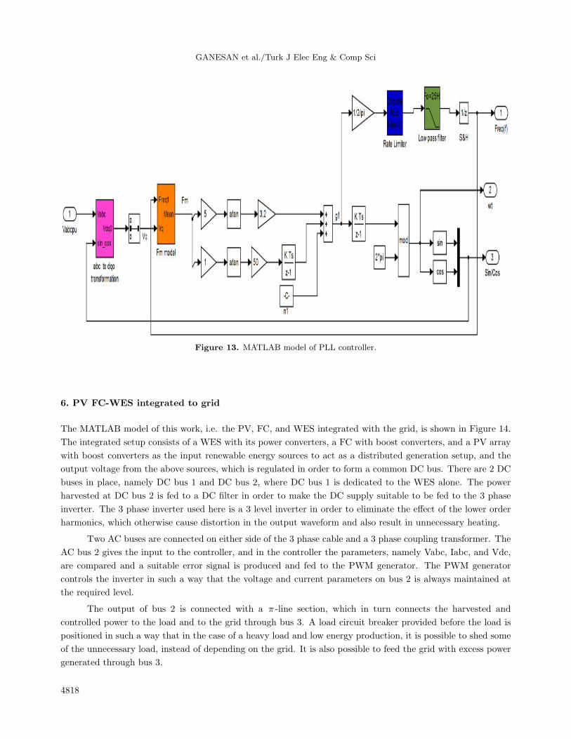
5. Mathematical model of the phase-locked loop controller

The phase-locked loop (PLL) controller shown in Figure 13 is a control system that generates an output signal

related to the phase of the input signal. The phase detector compares the phase of that signal with the phase of

the input periodic signal and adjusts the oscillator settings such that the input and output are locked with each

other. The PLL controller is used in this work where the abc parameters, in per unit values, are converted to

Vdq, and this is compared in the comparator by a further process and outputs of frequency, phase, and angular

speed of the turbine ωt are obtained as controlled parameters [19].

3.2 ∗[tan−1 (5 ∗ fm)

]+ ∫

[50 ∗ tan−1 (5 ∗ fm)

]+ n1 = s1 (38)

S1

(2

π

)= f (39)

|[(∫ s1) ∗ 2 ∗ π]| = ωt (40)

f ∗ [(∫ V q)− d2] + Cmp = fm (41)

Cmp = Vq +1

2

{(N −Nr)

N ∗ (Vq+1 − Vq) ∗ (N −Nr)

}(42)

Here, fm is mean frequency, f is measured frequency, N is the number of frequency samples per cycle, Nr is the

round-off value of N, and n1 is a constant.

4817

GANESAN et al./Turk J Elec Eng & Comp Sci

Figure 13. MATLAB model of PLL controller.

6. PV FC-WES integrated to grid

The MATLAB model of this work, i.e. the PV, FC, and WES integrated with the grid, is shown in Figure 14.

The integrated setup consists of a WES with its power converters, a FC with boost converters, and a PV array

with boost converters as the input renewable energy sources to act as a distributed generation setup, and the

output voltage from the above sources, which is regulated in order to form a common DC bus. There are 2 DC

buses in place, namely DC bus 1 and DC bus 2, where DC bus 1 is dedicated to the WES alone. The power

harvested at DC bus 2 is fed to a DC filter in order to make the DC supply suitable to be fed to the 3 phase

inverter. The 3 phase inverter used here is a 3 level inverter in order to eliminate the effect of the lower order

harmonics, which otherwise cause distortion in the output waveform and also result in unnecessary heating.

Two AC buses are connected on either side of the 3 phase cable and a 3 phase coupling transformer. The

AC bus 2 gives the input to the controller, and in the controller the parameters, namely Vabc, Iabc, and Vdc,

are compared and a suitable error signal is produced and fed to the PWM generator. The PWM generator

controls the inverter in such a way that the voltage and current parameters on bus 2 is always maintained at

the required level.

The output of bus 2 is connected with a π -line section, which in turn connects the harvested and

controlled power to the load and to the grid through bus 3. A load circuit breaker provided before the load is

positioned in such a way that in the case of a heavy load and low energy production, it is possible to shed some

of the unnecessary load, instead of depending on the grid. It is also possible to feed the grid with excess power

generated through bus 3.

4818

GANESAN et al./Turk J Elec Eng & Comp Sci

Figure 14. PV-FC-WES integrated to grid.

7. Voltage source converter controllers for power management

The VSC controller shown in Figure 15 controls the gate pulses of the 3 phase 3 level universal bridge, which is

responsible for DC/AC conversion and vice versa, so that the desired power sharing between the DGs and AC

grid is achieved

Figure 15. MATLAB model of a VSC controller.

4819

GANESAN et al./Turk J Elec Eng & Comp Sci

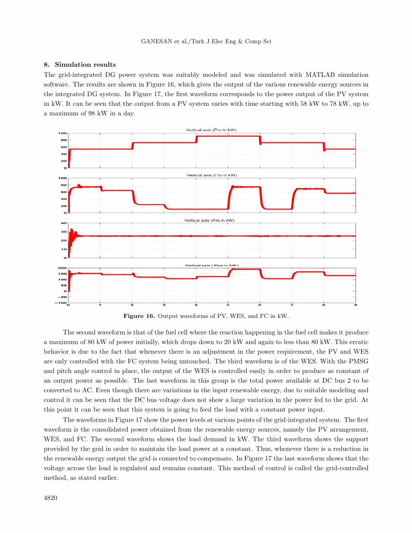
8. Simulation results

The grid-integrated DG power system was suitably modeled and was simulated with MATLAB simulation

software. The results are shown in Figure 16, which gives the output of the various renewable energy sources in

the integrated DG system. In Figure 17, the first waveform corresponds to the power output of the PV system

in kW. It can be seen that the output from a PV system varies with time starting with 58 kW to 78 kW, up to

a maximum of 98 kW in a day.

Figure 16. Output waveforms of PV, WES, and FC in kW.

The second waveform is that of the fuel cell where the reaction happening in the fuel cell makes it produce

a maximum of 80 kW of power initially, which drops down to 20 kW and again to less than 80 kW. This erratic

behavior is due to the fact that whenever there is an adjustment in the power requirement, the PV and WES

are only controlled with the FC system being untouched. The third waveform is of the WES. With the PMSG

and pitch angle control in place, the output of the WES is controlled easily in order to produce as constant of

an output power as possible. The last waveform in this group is the total power available at DC bus 2 to be

converted to AC. Even though there are variations in the input renewable energy, due to suitable modeling and

control it can be seen that the DC bus voltage does not show a large variation in the power fed to the grid. At

this point it can be seen that this system is going to feed the load with a constant power input.

The waveforms in Figure 17 show the power levels at various points of the grid-integrated system. The first

waveform is the consolidated power obtained from the renewable energy sources, namely the PV arrangement,

WES, and FC. The second waveform shows the load demand in kW. The third waveform shows the support

provided by the grid in order to maintain the load power at a constant. Thus, whenever there is a reduction in

the renewable energy output the grid is connected to compensate. In Figure 17 the last waveform shows that the

voltage across the load is regulated and remains constant. This method of control is called the grid-controlled

method, as stated earlier.

4820

GANESAN et al./Turk J Elec Eng & Comp Sci

Figure 17. Waveforms depicting power flow from the sources, load, and grid.

8.1. Effect of controller on the DG output power

The effect of the control circuitry implemented in the grid-integrated distributed generation system is shown

in Figure 18. It can be seen that the output of the DG system Pms follows the reference Pmsref . Thus, the

controller plays an important role in maintaining the output power profile of the DG system.

Figure 18. Effect of controller on the DG output.

4821

GANESAN et al./Turk J Elec Eng & Comp Sci

In contrast, Figure 19 shows what happens when the load demand is very high. Whenever the load is high

there is a feature implemented in this grid-integrated DG system in which load shedding or load curtailment is

automatically applied by the controller in order to match the DG generation and to provide grid independency.

For the above, the loads that are not essentially necessary when there is a dip in the DG generation are identified

and curtailment is applied while other critical loads are untouched. This ensures that the grid-integrated DG

system acts similar to a microgrid.

Figure 19. Waveforms depicting load curtailment feature.

9. Conclusion

From the previous sections, it can be seen that the grid-integrated hybrid DG sources of PV-FC-WES operate

satisfactorily as a combination of DGCM when the load is less than the renewable power generated and in

GCM when the load is greater than the renewable generation. The load shedding is implemented as and when

required. The DC bus voltage is maintained constant under all load conditions, satisfying the demand and

supply balance, and hence power management between DG sources, load, and grid is achieved.

The designed mathematical models and control strategies for PV, FC, WES, DC/DC converters, and

inverter along with the power controller and load controller effectively achieve the smooth and satisfactory

functioning of the grid-integrated hybrid system as mentioned above.

References

[1] Yang H, Wei Z, Chengzh L. Optimal design and techno economic analysis of a hybrid solar-wind power generation

system. Appl Energ 2009; 86: 163-169.

[2] Mahalakshmi M, Latha S. Modeling and simulation of solar photovoltaic wind and fuel cell hybrid energy systems.

Int J Eng Sci 2012; 4: 2356-2365.

[3] Wang C, Hashem NM. Power management of a stand-alone wind/photovoltaic/fuel cell energy system. IEEE T

Energy Conver 2008; 23: 957-967.

4822

GANESAN et al./Turk J Elec Eng & Comp Sci

[4] Khanh LN, Jae JS, Kim YS. Power management strategies for a grid connected PV-FC hybrid system. IEEE T

Power Deliver 2010; 25:1874-1882.

[5] Katiraei I, Iravani MR. Power management strategies for a microgrid with multiple distributed generation units.

IEEE T Power Syst 2006; 21: 1821-1831.

[6] Lu ZX, Wang CX, Min Y. Overview on microgrid research. Automation of Electric Power Systems 2007; 31: 100-107.

[7] Driesen J, Katiraei F. Design for distributed energy resources. IEEE Power Energy M 2008; 3: 30-40.

[8] Rauschenbach HS, Solar Cell Array Design Handbook. New York, NY, USA: Van Nostrand Reinhold Co., 1980.

[9] Ishaque K, Salam Z. An improved modeling method to determine the model parameters of photovoltaic modules

using differential evaluation. Sol Energy 2011; 85: 2349-2359.

[10] Villalva MG, Gazoli JR, Filho ER. Comprehensive approach to modeling and simulation of photovoltaic arrays.

IEEE T Power Electr 2009; 24: 1198-1208.

[11] Esram T, Chapman PL. Comparison of photovoltaic array maximum power point tracking techniques. IEEE T

Energy Conver 2007; 22: 2183-2189.

[12] Noguchi T, Togashi S, Nakamoto R. Short-current pulse-based maximum-power-point tracking method for multiple

photovoltaic and converter module system. IEEE T Ind Electron 2002; 49: 217-223.

[13] Jia J, Li Q, Wang Y, Cham Y T, Han M. Modelling and dynamic characteristics simulation of proton exchange

membrane fuel cell. IEEE T Energy Conver 2009; 24: 2375-2381.

[14] Hajizadeh A, Golkar MA. Intelligent power management strategy of hybrid distributed generation system. Int J

Elec Power 2007; 29:783-795.

[15] Leithead WE, Connor B. Control of variable speed wind turbines design task. Int J Control 2000; 13:1189-1212.

[16] Garcia Hernandez R, Garduno Ramirez R. Modeling a wind turbine synchronous generator. Int J Elec Power 2013;

2: 64-70.

[17] Ramtharan G, Jenkins N. Modelling and control of synchronous generators for wide range variable speed wind

turbines. Wind Energy 2007; 10: 231-246.

[18] Chen Z, Spooner E. Grid power quality with variable speed wind turbines. IEEE T Energy Conver 2001; 16: 148-154.

[19] Kim HW, Kim SS, Ko SS. Modeling and control of PMSG based variable speed wind turbine. Electr Pow Syst Res

2010; 80: 46-52.

4823