Embed Size (px)
Citation preview

MODELING AND SIMULATION ON THE YARD TRAILERS DEPLOYMENT IN THE MARITIME
CONTAINER TERMINAL
by
Yueqiong Zhao
A Thesis Submitted to the Faculty of
The College of Engineering and Computer Science
in Part ial Fu lfillment of the Requirements for the Degree of
Master of Science
Florida Atlantic University
Boca Raton, FL
May 2011

ODEL G D 1M L Tl0 0 THE ARD TRAILER DEPLOY E T THE
M RlTI CO T
by
ER TERM L
Yueqiong Zhao
Thi the is was prepared under the direction of the candidate s thesis ad isor Dr. E angelos I. KaisarDepartment of Ci it En ironmental and Geomatic Engineering and has been appro ed b the memb rsof her supervi ory committee. It was submitted to the faculty of the College of Engineering and Computer
cience and was accepted in partial fulfillment of the requirements for the degree of Master of cience.
P.D. carlatos, Ph.D.Chair Department of Ci
hgineering and Computer
-r.~Barr T. Ro n, Ph.D.Dean Graduate College
cience
II
iii
ACKNOW LEDGMENTS
I would like to express my thanks and appreciation to my advisor for providing me with the
opportunity to be a graduate student of his : Dr. Evangelos I. Kaisar. A lso, I want to thank him for his
guidance, encouragement and support during my graduate studies. His broad range of knowledge,
insightful critiques on crucial issues, and pursuit of theoretical precision provided excellent guidance
for shaping the ideas behind this work. Moreover, I appreciate h is warm personality and his willingness
to provide me with help when I met some difficulties in th is master program.
I would also like to thank the committee members, Dr. Yan Yong, Dr. Ramesh Teegavarapu, Dr.
Chingping Han, and Miss Jarice Rodriguez-Seda, for agreeing to serve on my thesis committee and for
sparing their invaluable time reviewing the manuscript and providing comments for the thesis. I owe
special gratitude to Dr. Ramesh Teegavarapu for all his help and suggestions for my model
development.
Additionally, I was very fortunate to be involved in a very great transportation group at Florida
Atlantic University. The students in this group deserve special thanks for taking the t ime to discuss my
research, to modify my paper work and the presentation, and help me with any questions I had.
What is more, I want to appreciate my parents who sent me to America to pursue further
education and for their love and support. They always offer me boundless love and support in my life.
iv
ABSTRACT
Author: Yueqiong Zhao
Title: Simulation on the Yard Trailers Deployment in a Container Terminal
Institution: Florida Atlantic University
Thesis Advisor: Dr. Evangalos I. Kaisar
Degree: Master of Science
Year: 2011
In recent years, there has been an exponential increase in container volume shipment within
intermodal transportation systems. Container terminals as part of the global port system represent
important hubs within this intermodal transportation system. Thus, the need to improve the operational
efficiency is the most important issue for container terminals from an economic standpoint. Moreover,
intermodal transportation systems, ports and inland t rans port facilities should all be integrated into one
coordinated plan. More specifically, a method to schedule different types of handling equipment in an
integrated way within a container terminal is a popular topic for researchers. However, not many
researchers have addresses this topic in relationship to the simulation aspect which will test feasible
solutions under real container terminal environment parameters.
In order to increase the efficiency of operations, the development of mathemat ical models and
algorithms is critical in finding the best feasible solution. The objective of this study is to evaluate the
feasible solution to find the proper number of Yard Trailers (YTs) with the min imal cost for the
container terminals. This study uses the Dynamic YTs operation s method as a background for
modeling. A mathematical model with various constraints related to the integrated operations among
the different types of handling equipment is formulated. This model takes into consideration both
serving time of quay cranes and yard cranes, and cost reduction strategies by decreasing use of YTs
with the specific objective of minimum total cost including utilization of YTs and vessel berthing. In
addition, a heuristic algorithm combined with Monte Carlo Method and Brute-Force Search are
employed. The early Stage Technique of Monte Carlo method is proposed to generate vast random
v
numbers to replicate simulat ion for real cases. The Brute-Force Search is used for identifying all
potential cases specific to the conditions of this study.
Some preliminary numerical test results suggest that this method is good for use in conjunction
with simulat ion of container terminal operation. The expected outcome of this research is a solution to
obtain the proper number of YTs for transporting containers with a minimum cost; thus, improving the
operational efficiency in a container terminal.
vi
MODELING AND SIMULATION ON THE YARD TRAILERS DEPLOYMENT IN THE
MARITIME CONTAINER TERMINAL
LIST OF TABLES....................................................................................................................................................... viii
LIST OF FIGURES ........................................................................................................................................................ ix
1. INTRODUCTION....................................................................................................................................................... 1
1.1 The Port and Container Terminal...................................................................................................................... 2
1.2 Cargo Transportation---Containerization ........................................................................................................ 6
1.3 Container Terminal Operations Description ................................................................................................... 9
1.4 Research Objective ............................................................................................................................................ 10
1.5 Thesis Organization ........................................................................................................................................... 11
2. LITERATURE REVIEW ........................................................................................................................................ 12
2.1 Container Terminal............................................................................................................................................ 12
2.2 Container Terminal Handling Operations ..................................................................................................... 13
2.2.1 Container Loading /Unloading Process................................................................................................. 13
2.2.2 Quay Crane Scheduling............................................................................................................................ 14
2.2.3 Yard Trailer Scheduling ........................................................................................................................... 16
2.2.4 Yard Crane Deployment .......................................................................................................................... 17
2.2.5 Integration of the Operation Scheduling ............................................................................................... 19
2.3 Optimization Algorithms .................................................................................................................................. 22
2.3.1 Genetic Algorithm..................................................................................................................................... 22
2.3.2 Tabu-Search ............................................................................................................................................... 23
2.3.3 Monte Carlo Methods............................................................................................................................... 25
2.3.4 Brute-Force Search ................................................................................................................................... 27
2.3.5 Branch and Bound Algorithm ................................................................................................................. 28
3. METHODOLOGY AND MODEL DEVELOPMENT ...................................................................................... 29
3.1 Preliminary .......................................................................................................................................................... 29
3.1.1 Traditional Operat ion ............................................................................................................................... 29

vii
3.1.2 Dynamic Operation ................................................................................................................................... 30
3.2 The Basic Idea of Modeling ............................................................................................................................. 32
3.3 Problem Assumptions and Analysis ............................................................................................................... 32
3.4 Modeling ............................................................................................................................................................. 36
3.4.1 Notations and Variables ........................................................................................................................... 36
3.4.2 Mathemat ical Analysis and Objective Function .................................................................................. 37
3.4.3 Constraints.................................................................................................................................................. 38
3.5 Some Discussion ................................................................................................................................................ 39
4. SIMULATION AND RESULT ANALYSIS....................................................................................................... 41
4.1 Simulation Idea and Algorithm ....................................................................................................................... 41
4.2. Computation ...................................................................................................................................................... 46
4.2.1. Test Design and Results .......................................................................................................................... 46
4.2.2. Other Numerical Tests and Analysis .................................................................................................... 51
4.3. Summary ............................................................................................................................................................ 52
5. CONCLUSION.......................................................................................................................................................... 54
5.1 Major Contributions of the Study ................................................................................................................... 54
5.2 Limitations of the Study ................................................................................................................................... 55
5.3 Recommendations for Future Work ............................................................................................................... 55
APPENDIX..................................................................................................................................................................... 57
REFERENCES............................................................................................................................................................... 69
viii
LIST OF TABLES
Table 1 Input Data ................................................................................................................................................ 47
Table 2: Mean Value of 10000 Simulat ions Runs .......................................................................................... 48
Table 3: The Results with Different Unit Cost ................................................................................................ 51
Table 4: The Results from Different Inbound Volume and Number of QCs ............................................. 52
Table 5: The Results with Different Unit Time of QCs ................................................................................. 52

ix
LIST OF FIGURES
Figure 1: A Typical Yard Allocation (Eric Ting).............................................................................................. 5
Figure 2: A Typical Container Allocation in a Yard ........................................................................................ 6
Figure 3: Container Volume (Peter Smeetes, 2009) ......................................................................................... 8
Figure 4: Container Projections 2008-2012 (AXS-Alphaliner, 2008)......................................................... 8
Figure 5: Typical Flow Containers in Terminal Operat ions (W.c.Ng, K.L.Mak, 2003) .......................... 10
Figure 6: Typical Container Yard Layout of a Container Terminal (W.C.Ng., 2005) ............................. 13
Figure 7: Quay Crane: Dual-Trolley Cranes (Dirk Steenken, et al., 2004) ................................................ 15
Figure 8: A Layout of a Multimodal Container Terminal Kozen and Preston, 1999 ....................... 20
Figure 9: Tabu Search Short-term Memory Component (Fred Glover, 2001)........................................... 24
Figure 10: Selecting the Best Admissible Candidate (Fred Glover, 2001)................................................. 25
Figure 11: Tradit ional Operations of the Container Terminal (Liu, 2009) ................................................. 30
Figure 12: Tradit ional Method for Yard Trailer Operations (Zeng, et. al, 2009) ...................................... 31
Figure 13: Dynamic Operat ions YTs Share for Different Sh ips (Zeng, et. al., 2009) ........................... 31
Figure 14: One Circle of YT Travel Route ...................................................................................................... 33
Figure 15: The Relationship between the Cost Function and the Number of YTs.................................... 35
Figure 16: Flow Chart of the Algorithm ........................................................................................................... 43
Figure 17: One Circle of YTs Travel Route..................................................................................................... 44
Figure 18: Scenario 1 Results: the Cost of YTs in Use for Each QC: VC(k)............................................. 48
Figure 19: Scenario 1 Results: the Cost of Mooring in the Berth of Unloading Vessel: MC(k) ............ 49
Figure 20: Scenario 1 Results: the Total Cost: Z ............................................................................................ 49
Figure 21: Ten Random Simulation Results .................................................................................................... 50
1
1. INTRODUCTION
Today, we see a renewed focus on the intermodal freight transportation. The term of intermodalis m,
especially for the freight transportation, can be simply defined as a single-b ill-shipment uses multimodal
transportation mode. The intermodalism originated in marit ime transportation, which is a very huge part of
the global transportation network, with the development of the container almost five decades ago.
Moreover, today‟s globalization of trade and the subsequent breakdown of trade barriers have spurred
tremendous growth in marine container traffic. Ports, which serve as hubs of container transshipment, p lay
critical roles in the marine transportation network.
Technological improvements in recent years have made it essential to plan the transportation system
of a developing country as a whole, in order to achieve a balance between the capacities of the various
ports. In marit ime transport, it is sometimes possible, particularly fo r bulk and unitized cargo, such as a
container, to include the shipping. Thus, ports and inland transport facilit ies work best when they are
included into one coordinated plan for intermodal conveyance. In other cases, the ship traffic is not under
the control of the planner, and it is only possible to coordinate the port facilities with those of inland
transport and distribution (Port development: A handbook for planners in developing countries , 1985).
Considering the containers ‟ transportation within the port, only planning the vessel transportation without
considering the connection with terminal facilit ies may lead to serious faults in communication. Because
the container freight traffic is rapidly growing, efficiency in container handling operations , which includes
the utilization of resources in the port, is so important for the demand of high quality services from
container terminals. Methodological advances regarding container terminal operations have considerably
improved through much research. However, in the past research, most focus on a single type of equipment
without considering the sequence of the different equipment in the systems. Also, the connectivity of
handling operations between quaysides and yards in container terminals is the most critical issue, which
2
may cause delay problems to arise with significant impact on the whole container handling processes, so
the efficient solutions for this problem are crit ical for systems to have efficient and productive performance.
1.1 The Port and Container Terminal
A port is a site next to a body of water containing one or several harbors where marine transportation
modes can dock and transport people or shipments to or from land. Seaport locations are chosen to
optimize access between land and water in regards to business purposes and refuge from hazardous weather.
Deep water ports are less common, but can serve a larger variety of vessels . Since ports have been very
influential h istorically, they frequently dominate the local economy and vary widely.
As the concept of intermodal transportation has become more efficient, economical, and practica l, a
port is treated as an importation element in the global transportation market by serving as a multi-modal
interface, which often links the sea and land transportation.
Ports often have cargo-handling equipment for use in loading and unloading vessels, and some ports
feature canals, which allow vessels further movement in land. Access to the intermodal transportation, such
as railways and land transportation, is critical to a port so that passengers and cargo can also move further
inland beyond the port area.
Because the international demand for containers is rising, container terminals have become an
important mode in the global transportation network and have become a v ital ro le within the intermodal
transportation system. A nautical container terminal is normally a component of a larger port; it is a facility
where containers are transferred among different transportation modes for continued distribution. The big
marine container terminals are similar to key harbors because they transfer containers within a global
transportation network. “Marit ime container terminals provide many functions, such as transship, transfer,
or storage. As the demand for international trade and global logistic services continues to increase
substantial investments and improve ments in both physical capacity and operational efficiencies are
necessary to enhance terminal productivity” (Eric Ting “ Container Terminal Operation and Cargo
Handling”).
Cargo passes through a container terminal usually in three different ways: it may be imported,
exported, or transshipped: moved from one vessel to another. containers terminals can be designed in base

3
of the concern of handling, storage, and possibly loading or un loading of cargo into or out of containers,
and where containers can be picked up, dropped off, stored, maintained, unloaded or loaded from one mode
of transportation to another , that is, vessel, truck, rail, even plane. Being categorized by their ownerships,
container terminals can be generally classified into five part: public terminals, carrier-leased dedicated
terminals, terminal-operator built and operation terminals, carrier built and operation terminals, and joint
venture of carriers and terminal operators , these different type of terminals are explained in following by
Eric Ting;
Public terminals
Shipping lines can share the facilit ies and operations of public terminals with each other. They are
charged at tariff rates. The first come, first serve principle is usually used, and there is no priority in berth
usage except by paying the priority fee. Container handling and other charges are calculated at common
tariff rates or paid at quantity discount rates based on the container volume if it is over the fixed quantity
agreed upon in contracts. The terminal in Singapore (PSA before 1997) is categorized into this class.
Carrier-leased dedicated terminals
Emphasizing on their exclusive use, carriers make the long-term lease contracts with the port
authorities. Carriers pay rents and facility charges and have priority and right for berth usage. Carriers can
purchase or set up container handling facilit ies at their own account to compensate for rents and facility
charges. Kaohsiung, Keelung (some parts of the port), Kobe, Yokohama, and Tokyo are categorized into
this operation pattern.
Terminal-operator built and operation terminals
A terminal operator builds an operation terminal o r invests in the construction and handling facilit ies.
Hong Kong (HIT, MTL, CHT), Tianjin (CSXOT), and Singapore (PSA after 1997) are categorized into this
category.
Carrier built and operation terminals
Carriers will build container terminals or inves t directly in the construction. The handling facilities
and the operations of the container terminal are managed by the carriers. Except with the usage of their own
fleet, the carriers are authorized to provide other shipping lines with berthing and container handling
services. Taipei Port (invested by Yang Ming Line, Evergreen, Wan-Hai),Qingdao (Zhunguang, Kuaikuei,

4
Tiasing), and Malaysia (PTP) are categorized into such operation patterns.
Joint venture of carriers and terminal operators
Both shipping lines and terminal operators establish a company to jo int venture together, by making a
joint investment in building or leasing of the container terminals or investing directly in the construction
and handling facilities. Shanghai (Yangshan terminals and Zhunghai terminals) and Shenzhen belong to
this group.
Container terminals vary in location, size, operation methods, management, kinds of equipment,
arrangement and other aspects, which means that there are many factors affecting container terminal design
and decision making in the early stages. As Hwarng (1998) mentioned, the interrelationship between
various activities in container terminals usually leads to a terminal operation problem that is dynamic in
nature and with stochastic behavior.
In the container terminal, the yard area, as a large component of it, provides many functions within
the system. These functions include the container unloading/loading operations for storage, transshipment
operations, or turnaround. Hence, any type of container flow will be served in the yard. Figure 1 shows the
regular container terminal allocation. Introduced by Eric Ting in his study, the container yard usually
includes several types:

5
Figure 1: A Typical Yard Allocation (Eric Ting)
(1) Marshalling Yard (MY), which is located close to the berth, used to improve the efficiency of
loading/unloading operations for vessels. The export containers are stacked according to certain
rules or plans in this yard before loading to the vessel. And for the import containers, they are also
stacked in this yard as a temporary method. They are usually served randomly.
(2) Back yard, which is not contained in every terminal, is utilized for turnaround, storage of containers,
especially for heavy and empty containers. It is always treated as the connection area between the
whole terminal and the land, served for the containers‟ distribution.
(3) Empty containers yard, especially for the collection, store, and turnaround of empty containers in case
of shortage area of the first two types of years. Both back yard and empty containers yard can be called
into Container Yard (CY)
In the whole terminal, there is another area: Container Freight Station (CFS). It usually contains one
or more sheds, warehouses or uncovered storage areas where cargoes are loaded into or unloaded from
containers and may be temporarily stored in the sheds or warehouses.

6
Currently, in most studies, the marshalling yard is called yard, which is close to the berth. As shown
in figure 2: “a typical yard consists of several blocks, and each b lock consists of 20±30 yard -bays. Each
yard-bay contains several (usually 6) rows. Each ground slot, denoted as a rectangle in the diagram, can
store 5-7 containers. When an outside truck delivers an outbound container to a yard, a transfer crane picks
it up and stacks it in a yard-bay” (Kap Hwan Kim, et al. 1999).
Figure 2: A Typical Container Allocation in a Yard
1.2 Cargo Transportation---Containerization
According to the International Organization for Standardizat ion (ISO), containerization is a network
of intermodal cargo transportation using typical intermodal containers. These can be transported by vessels,
airplanes, railway trains, and ground vehicles. Containerizat ion brings an important improvement to the
field of logistics, which has revolutionized freight transportation in the last century. The transportation of
cargo containers originated at the beginning of the 19th century. These containers can be transferred among
different methods of transportation, such as railroads, vessels, or trucks. The containers used in the past
were much s maller than the containers being used today. In the 1920s, the Milwaukee Railway and the
Chicago North Shore companies began using different vehicles, such as plane cars, to transport cargo.
Shortly after, Seatrain Lines started carrying railroad boxcars onto ships to transport cargoes between Cuba
and New York. In the 1950s, these plane cars were furnished with new decks. In 1951, containers were
transported for the first time by vessels between Alaska and Seattle. The first container ship was
Yard Trailers
Crane
Slot
Block
Tier
Row Bay
7
constructed in Canada in 1955. In its first voyage, it handled 600 containers between Skagway, A laska and
North Vancouver. This method of transportation gradually achieved intermodalism. In 1956, Malcolm
McLean developed the standard containers which are used today. They could be moved by cranes onto a
vessel or a truck, making transfer operations more efficient.
Currently, there are two standard containers sizes: the twenty-foot equivalent unit (TEU = 20' length
x 8' width x 8.5' height) and the forty-foot equivalent unit (FEU = 40' x 8' x 8.5'). Instead of using the Dead
Weight Tonnage (DWT) to define capacity units for all container ships, TEU and FEU are widely used
today.
Vessel designs and harbor capacities have been developed to meet current container needs . Therefore,
containerizat ion and intermodalis m have completely revolutionized the transportation of cargo. Today's
global fleets are made up of 3,375 containerships with 7.2 million TEUs. According to Chris Koch,
president of the World Shipping Council, containerizat ion has made global business transportation smooth
and more efficient. In effect, the development of containers allowed the shipping industry to grow
significantly (P. Jaime Tetrau lt, 2010).
Expansion in container trade is mostly driven by economic growth, and today‟s focus of
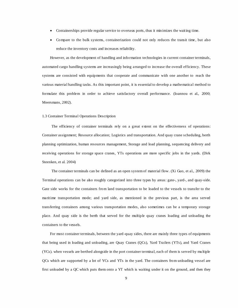
intermodalis m has been on containerization. By the end of October 2008, there are 4627 container vessels
with a total capacity approximately to 12.2 million TEUs [AXS-Alphaliner, 2008]. Therefore,
containerizat ion has become more important as the integral part o f logistics. It has rev olutionized the cargo
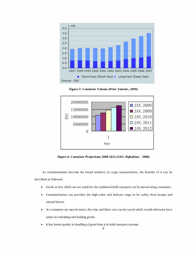
shipping. According to the CBS data from Netherland, from 2002-2007, only the container trade to
Netherland is increasing every year showed in figure 3. And based on the prediction, in the next coming
years, the container trade will be continually rising shown in figure 4. Today, nearly 90% of global trade
volume is shipped in containers. One fourth of world‟s total containers start from China.
8
Figure 3: Container Volume (Peter Smeetes, 2009)
0
5000000
10000000
15000000
20000000
1
YAER
TEU
JAN.2008
JAN.2009
JAN.2010
JAN.2011
JAN.2012
Figure 4: Container Projections 2008-2012 (AXS-Alphaliner, 2008)
As containerization become the broad tendency in cargo transportation, the benefits of it can be
described as followed:
Goods in lots which are too small for the traditional bulk t ransport can be moved using containers.
Containerizat ion can provides the high-value and delicate cargo to be safety from human and
natural factors
As containers are moved intact, the t ime and labor cost can be saved which would otherwise have
spent on unloading and loading goods.
It has better quality in handling of good than it in bulk transport systems.
Year
9
Containerships provide regular service to overseas ports, thus it min imizes the wait ing time.
Compare to the bulk systems, containerization could not only reduces the transit time , but also
reduce the inventory costs and increases reliability.
However, as the development of handling and information technologies in current container terminals,
automated cargo handling systems are increasingly being arranged to increase the overall efficiency. These
systems are consisted with equipments that cooperate and communicate with one another to reach the
various material handling tasks. As this important point, it is essential to develop a mathematical method to
formulate this problem in order to achieve satisfactory overall performance. (Ioannou et al., 2000;
Meersmans, 2002).
1.3 Container Terminal Operations Description
The efficiency of container terminals rely on a g reat extent on the effectiveness of operations:
Container assignment; Resource allocation; Logistics and transportation. And quay crane scheduling, berth
planning optimization, human resources management, Storage and load planning, sequencing delivery and
receiving operations for storage space cranes, YTs operations are more specific jobs in the yards. (Dirk
Steenken, et al. 2004)
The container terminals can be defined as an open system of material flow. (Xi Guo, et al., 2009) the
Terminal operations can be also roughly categorized into three types by areas: gate-, yard-, and quay-side.
Gate side works for the containers from land transportation to be loaded to the vessels to transfer to the
marit ime transportation mode; and yard side, as mentioned in the previous part, is the area served
transferring containers among various transportation modes, also sometimes can be a temporary storage
place. And quay side is the berth that served for the multip le quay cranes loading and unloading the
containers to the vessels.
For most container terminals, between the yard -quay sides, there are mainly three types of equipments
that being used in loading and unloading, are Quay Cranes (QCs), Yard Trailers (YTs), and Yard Cranes
(YCs). when vessels are berthed alongside in the port container terminal, each of them is served by multiple
QCs which are supported by a lot of YCs and YTs in the yard. The containers from unloading vessel are
first unloaded by a QC which puts them onto a YT which is waiting under it on the ground, and then they
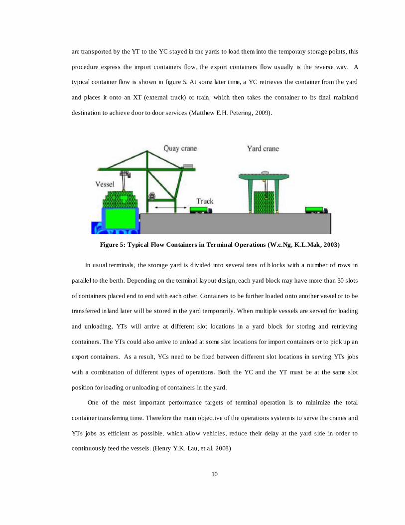
10
are transported by the YT to the YC stayed in the yards to load them into the temporary storage points, this
procedure express the import containers flow, the export containers flow usually is the reverse way. A
typical container flow is shown in figure 5. At some later t ime, a YC retrieves the container from the yard
and places it onto an XT (external truck) or t rain, which then takes the container to its final mainland
destination to achieve door to door services (Matthew E.H. Petering, 2009).
In usual terminals, the storage yard is d ivided into several tens of b locks with a number of rows in
parallel to the berth. Depending on the terminal layout design, each yard block may have more than 30 slots
of containers placed end to end with each other. Containers to be further loaded onto another vessel or to be
transferred in land later will be stored in the yard temporarily. When multip le vessels are served for loading
and unloading, YTs will arrive at d ifferent slot locations in a yard block for storing and retrieving
containers. The YTs could also arrive to unload at some slot locations for import containers or to pick up an
export containers. As a result, YCs need to be fixed between different slot locations in serving YTs jobs
with a combination of d ifferent types of operations . Both the YC and the YT must be at the same slot
position for loading or unloading of containers in the yard.
One of the most important performance targets of terminal operation is to minimize the total
container transferring time. Therefore the main object ive of the operations system is to serve the cranes and
YTs jobs as efficient as possible, which allow vehicles, reduce their delay at the yard side in order to
continuously feed the vessels. (Henry Y.K. Lau, et al. 2008)
Figure 5: Typical Flow Containers in Terminal Operations (W.c.Ng, K.L.Mak, 2003)
11
1.4 Research Objective
The major goal of this study is to simulate an integrated handling system and to find an efficient
solution algorithm for Yard Trailer (YT) arrangement. In order to achieve the purpose of this study, the
following objectives will be pursued:
Development of a mathematical model for Yard Trailers arrangement, which is considered under
the conditions of both loading and unloading synchronously. This model will be used for finding
the exact solution.
Development of an algorithm to reach a general simulation for searching for the best number of
YTs in specific cases. The basic stage technique of Monte Carlo method will be used to generate
the random number to simulate, and the Brute-Force method will be used to find the best solution.
For the final best feasible solution, the proper number of YTs in regards to minimal cost will be
presented.
1.5 Thesis Organization
The rest of this thesis is organized as follows: Chapter 2 presents a survey of research work closely
related to this thesis‟s field. Charter 3 addresses the problem statement with discussing the important issues
of handling system in the container terminal and the developed model, discussion follows based on
constraints. Chapter 4 provides and simulation algorithms and the results of test studies in order to examine
the model performance. Charter 5 summarizes the contributions and limitations of the work in this thesis ,
and indicates some possible future researches.
12
2. LITERATURE REVIEW
Issues related to container terminal have gained attention recently due to the increased importance of
marine transportation systems. There are several aspects in this field. In following, a brief review of
existing studies related to this topic is provided in d ifferent parts, which are container terminal, handling
operations in the container terminal, optimization algorithms which were popular employed in researches. .
2.1 Container Terminal
Modern container terminals are not passive points of interface between sea and land transport, the
container terminals have been treated as a logistics centre acting for intermodal interchange. The
importance of container terminals to the economic and social d imensions of a community, nation, or region
is significant. Better performances of container terminals , could contribute in increasing trade and
development of national economies (W. Winklemans and E. Van de Voorde, 2002).
Container terminals can be described as open systems of material flow with two external interfaces.
These interfaces are the quayside with loading and unloading of vessels, and the landside where containers
are loaded and unloaded on/off trucks and trains. Usually, container terminals are described very
specifically with respect to their equipment and stacking facilities.
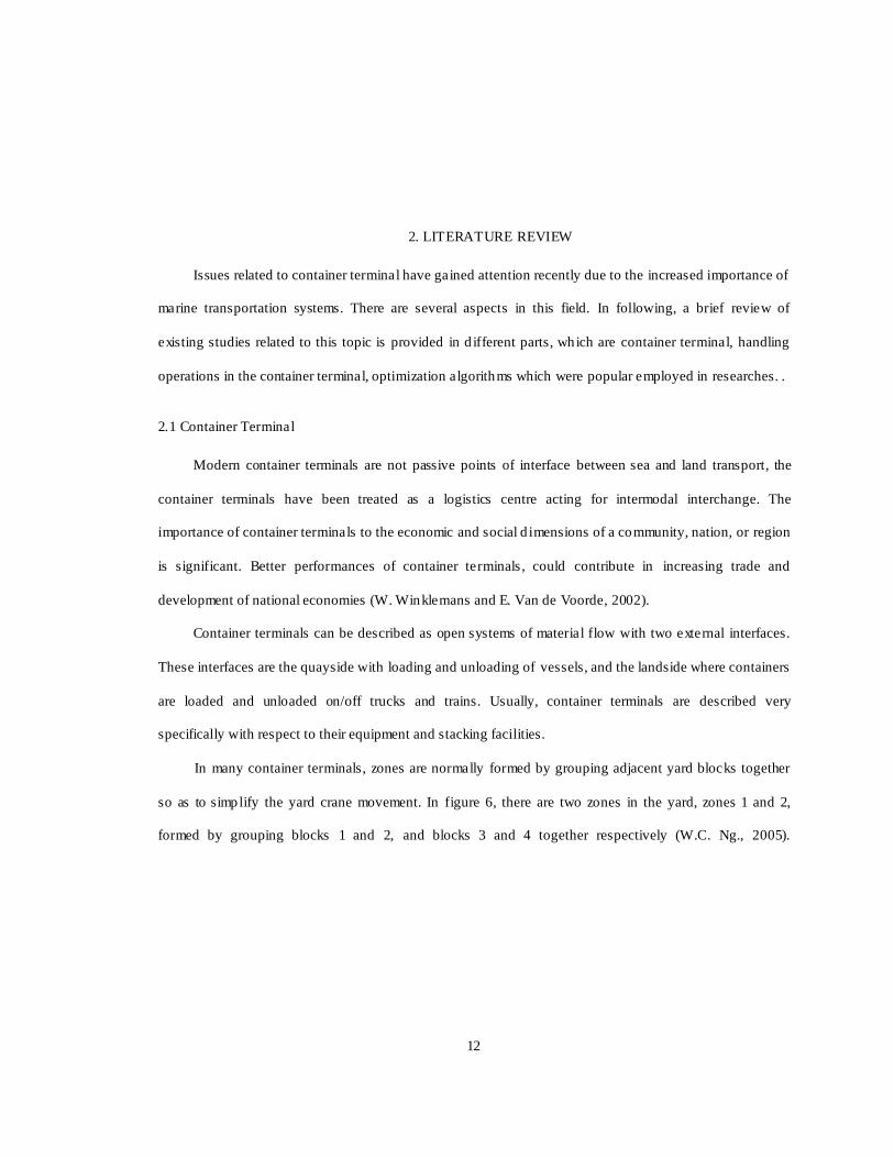
In many container terminals, zones are normally formed by grouping adjacent yard blocks together
so as to simplify the yard crane movement. In figure 6, there are two zones in the yard, zones 1 and 2,
formed by grouping blocks 1 and 2, and blocks 3 and 4 together respectively (W.C. Ng., 2005).
13
Figure 6: Typical Container Yard Layout of a Container Terminal (W.C. Ng., 2005)
The yard stacks, vessels, trains, and trucks belong to the category „stock‟. Stocks are statically defined
by their ab ility to store containers while from a dynamic point of view . a stowage (or loading) sequence is
necessary to instruct that how and where containers would to be stored. There is no principal d ifference
between these different types of stocks but only a difference in capacity and complexity. (Dirk Steenken, et
al., 2004).
2.2 Container Terminal Handling Operations
There are many different handling operations in the container terminals. Researchers have been
explored many studies in different parts which can be separated into different aspects depends on the
serving procedure. The related research is summarized into the next several groups.
2.2.1 Container Loading /Unloading Process
The container-loading problem has been explored for many years by researchers . Avriel and Penn
(1993) developed a simplified mathematical model for the stowage-planning problem based on 0-1 b inary
linear programming. It t ried to minimize shifting operations without considering stability constraints.
Avriel et al. (1998) continued to study this problem as a two-d imensional stacking problem, and a heuristic
algorithm was developed with the objective of min imizing the number of shift ing operations. However, it

14
assumed that there is only one large cargo bay in a vessel without considering constraints related to batch
covers and the stability of the vessel.
Kaisar (1999) studied the containership operation. In his study, a vessel visits a series of ports, it was
totally empty at the first port the vessel by assumption, and then a mathematical model presented by
considering varies factors, such as longitudinal moment, trim. This model deal with containers with same
dimensions, different weights, and assumes the container first assigns containers to available positions, if it
is not satisfied, then re-assigned. Mix Integer Programming (MIP) with the objective of min imizing the
extra container handling was developed in this study. And he continued this problem in h is PhD
dissertation (2006), he addressed the vessel turnaround time at container terminals is an important measure
of a port‟s efficiency and attractiveness. The speed and quality of load planning affect the length of
turnaround time considerably, and the stability of the vessel and a variety of other stochastic processes
should be considered. A MIP model was also formulated fo r the stowage-planning model to minimize extra
shifting. And a heuristic algorithm was developed to solve this problem.
The key contributions of this dissertation are as follows.
(1) A mathematical model is developed by considering real life constraints and considering
loading/unloading along the entire voyage.
(2) A second mathemat ical model is formulated to obtain a lower bound on the value of the objective
function of the exact solution.
(3) A heuristic algorithm is developed that is guide by practical considerations that account for the
structure of the stowage-planning problem.
(4) All proposed mathematical models and heuristic are validated with experimental results. In all cases,
these results demonstrate the stability, flexib ility and efficiency of the model, and establish its potential
as a versatile and practical method for large scale container loading.
2.2.2 Quay Crane Scheduling
Concerning cranes, different types are used at container terminals. The Quay Cranes (QCs) which are
worked for loading and unloading vessels play a major role. Two types of QCs can be d istinguished:
single-trolley cranes and dual-trolley cranes. They move the containers from the vessel to the shore either

15
putting them on the quay or on a vehicle (and vice versa for the loading cycle). There is a picture of QCs
provided by Dick in 2004, shown in figure 7
Figure 7: Quay Crane: Dual-Trolley Cranes (Dirk Steenken, et al., 2004)
Various studies on the scheduling of QCs were done by different researches. Daganzo (1989) studied
the static and dynamic QC scheduling problems for multiple container vessels. He firstly assumed that
container vessels were divided into holds, and only one QC could work on a hold at a time. QCs could be
moved freely and quickly among holds, and container vessels could not depart until all their holds had been
handled. The objective was to serve all these container vessels, while min imizing their aggregate cost of
delay. And then exact and approximate solution methods for QC scheduling were presented. Later, a
branch and bound algorithm was developed for further study on the same problem by Peterkofsky and
Daganzo in 1990. However, both of these two papers overlooked that the QCs could unrealistically cross
over each other.
Lim et al. (2004) continued to consider this problem by adding non-interference constraints. They
assumed that containers from a given area on a container vessel, and there was a profit value when a job
was assigned to a QC. The objective was to find a crane-to-job matching which maximized the total profit.
A probabilistic Tabu Search algorithm and a squeaky wheel optimization heuristic were proposed for
solving the problem. However, it is difficu lt to define a profit value associated with a crane -to-job
assignment in practice, and hence this research cannot be applied in port container terminals easily.
16
Kim and Park (2004) d iscussed the QC scheduling problem with non-interference constraints
(QCSNIP). Only single container vessel was considered. Firstly, they defined a task as an unloading or
loading operation for a collection of adjacent slots on one single container vessel. The object ive was to
minimize the weighted sum of the makespan of the container vessel and the total complet ion time of all
QCs. And then they proposed a branch and bound algorithm and a heuristic algorithm called „greedy
randomized adaptive search procedure (GRASP) ‟ for the solution of the QC scheduling problem. But the
computational complexity of th is problem was not discussed in this study.
Lee et al continued to analysis this problem in 2008. Firstly they developed a MIP model with the
objective of minimizing the makespan of handing one single container vessel, which was the latest
complet ion time among all holds according to configuration of container vessels. Secondly , they discussed
the computational complexity of the QCSCIP and proved it was NP -hard problem by 4 steps. Third ly, they
proposed an approximat ion algorithm to obtain near optimal solution, and then evaluated by twenty
experiments, the results showed the proposed algorithm was effective and efficient in solving the QCs
scheduling.
2.2.3 Yard Trailer Scheduling
Nishimura et al. (2005) considered dynamic YTs scheduling problem in his model. A heuristic was
developed and a wide variety of computational experiments were conducted. The results of the experiments
demonstrated that the dynamic routing reduced travel d istance and generated substantial savings in the
trailer fleet size and overall cost (15% reduction). The contribution of this study is the development of a
new routing plan achieving container handling cost savings for a terminal. However, the loading and
unloading operations of QCs are not considered, and thus it cannot realize the operation coordination
between different QCs.
Truck scheduling and storage allocation, as two separate sub-problems in port operations, have been
deeply studied in past decades. However, from the operational point of view, they are h ighly
interdependent. Storage allocation for import containers has to balance the travel time and queuing time of
each container in yard. Cao, et al. (2008) proposed an integer programming model handling these two
problems as a whole. The objective of this model was to reduce congestion and waiting time of container

17
trucks in the terminal so as to decrease the makespan of discharging containers. As the complexity of the
problem, a genetic algorithm and a greedy heuristic algorithm were developed to attain near optimal
solutions. It showed that the heuristic algorithm can achieve the optimal solution for small -scale problems.
The solutions of small-and large-scale problems obtained from the heuristic algorithm are better than those
from the genetic algorithm. Der-Horng Lee, et al. (2008) continued to propose a novel approach that
integrates these two problems into a whole. The objective was to minimize the weighted sum of total delay
and the total travel time of yard trucks. Due to the intractability of the proposed problem, a hybrid insertion
algorithm is designed for effective problem solutions. Computational experiments are conducted to
examine the key factors of the problem and the performance of the proposed heuristic algorithm.
2.2.4 Yard Crane Deployment
The Yard Cranes (YCs) operations were commonly organized into 3 levels by many researchers.
(1) Before the start of operations, the number of YCs to be deployed for the shift is decided with reference
to the number of QCs that will serve the vessels, the number of YTs expected for import/export
containers and the amount of container re-shuffling work within the yard.
(2) YCs are distributed to different rows of the yards.
(3) YCs deployment aims to determine the order in which the vehicle (the loading or unloading jobs) is
served by the mult iple cranes which are sharing the workload in the row of yard blocks.
Kim and Kim (1999) p roposed the problem of routing single YC for loading operations of a vessel as
Mixed Integer Programming (MIP) model, and in 2003, they continued this problems but solved by
presented Genetic Algorithm (GA) as shown by numerical experiments. However, the contribution from
them just focused on the vessel loading operations in not useful for large terminals with many berths.
Zyngiridis, et al. (2005) proposed linear integer programs for one or two equal sized Automated
Stacking Cranes routes scheduling in a single block working with straddle carriers. The objective was to
minimize the total travel d istance of cranes while g iving priority to export. The big contribution of this
work was considering the straddle carriers. The difference between them from normal vehicles was that
straddle carriers can pick up and place down the containers by themselves while normal vehicles need
cranes in carrying out these operations.
18
Lee, et al. (2007) presented the problem of loading operations with two YCs serving one QC. A
simulated annealing algorithm was addressed with the objective which is min imizing the total loading time
at the stack area.
There are some but not abundant works which focused on the inter-block level YC deployment.
Rubber Tired Gantry Cranes (RTGCs) are the most frequently used equipment in yards for container
handling. The efficiency of yard operations highly depends on the productivity of these RTGCs. Zhang, et
al. (2002) addressed the RTGC deployment to find times and routes for RTGC movements. Firstly, given
the forecasted workload of each b lock in each period o f a day, the objectives were to find the times and
routes of cranes movement among blocks and minimize the total delayed workload in the yard. The
problem is formulated as a mixed integer programming (MIP) model and solved by Lagrangean relaxat ion.
To improve the performance of this approach, the authors developed this Lagrangean relaxation model by
adding additional constraints and modify the solution procedure accordingly. Computational experiments
showed that the modified Lagrangean relaxation method worked well and could reach good solutions in a
short time. Cheung, et al. (2002) also used MIP model for the problem about allocating YCs among yard
blocks to schedule inter-block movements. But they did not show simulation to test performances.
W.C.Ng, K.L.Mak (2005) addressed the problems of scheduling YCs to perform a g iven set of
loading/unloading jobs with different ready times within movement zone. Firstly, they formulated this
problem as a MIP model with the objective that minimizing the sum of job waiting times. Secondly, they
noted that for this case, YCs deployment was a problem of non-reemptive scheduling with different job
ready times on a single machine to min imize total completion time and the scheduling problem is an NP-
complete problem, a branch and bound algorithm was proposed to solve it optimally, and in order make it
be more efficient, there was an efficient and effective heuristic used for searching the lower and upper
bound. Finally, the small size number randomly generated problems were s olved by CPLEX, the larger size
number randomly generated test problems were solved by the branch and bound algorithm. The
computation results have shown that the algorithm works well for most of the test problems.
XiGuo, et al, (2008) considered the problem of partition ing h blocks in the same row in the container
storage yard into k non-overlapping zones, there was two assumptions in the YC d ispatching problem:
Each vehicle job handles one container only and real time information on the location of each vehicle with
19
becoming to the row of yard b locks for the storage/retrieval job is available. The objective of partit ioning h
blocks in the container storage yard into k non-overlapping zones was to minimize the average job waiting
time for reducing the QC wait ing time for vehicles so as to reduce vessel turnaround time. The problems
solved by partition algorithm and simulated by real t ime data. Computation test results showed that
choosing the best performing partition p lan based on the optimized service sequ ence will be ab le to
produce the smallest vehicle wait ing time, which will help maintain the continuous feeding of the QCs by
the vehicles and thus reduce the vessel turnaround time. The authors also recommended that developing
techniques such as dynamic p rogramming to remove repeated computation in the workload part ition
process is one is useful for future work.
2.2.5 Integration of the Operation Scheduling
The operation efficiency of container terminals depends on the coordination of different sub -
processes, in order to improve the operation quality in the container terminals overall, the integrated
handling system which combines those different necessary equipments. However, the optimization models
mentioned above just focus on a single equipment operation optimization cannot optimize the cooperation
activities.
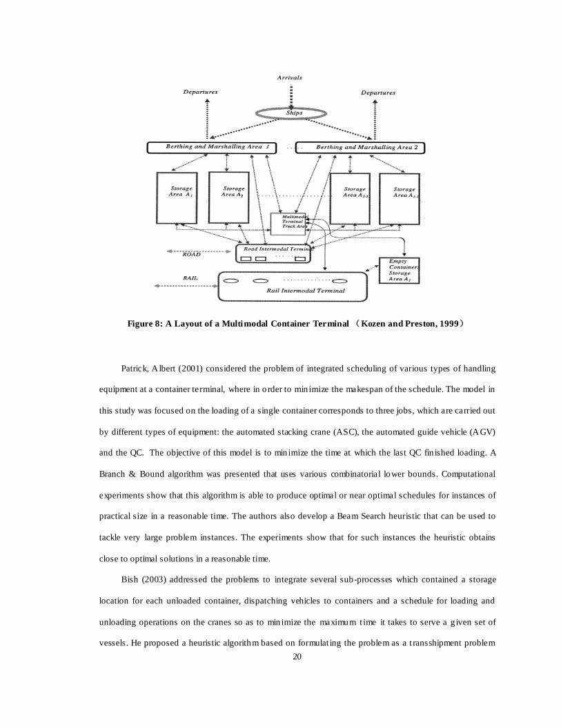
Kozan and Preston (1999) first descript the layout of a mult imodal container terminal by drawing a
map, in figure 8, and they developed established a MIP model to optimize both of the loading and
unloading. In this model, two areas were involved: storage strategy of the containers in the yard and
loading and unloading orders. The objective of the model was to minimize the stay time of a vessel in a
berth, and the vessels berthing time were employed as a constraint. The storage points were described by
matrix based on Cartesian coordinates. Then, a genetic algorithm was used to obtain near-optimal solutions
in reasonable time. the authors also recommended that The possibilities of using other heurist ic techniques,
like simulated annealing, neural networks, or Tabu search, should be examined in future research, to see if
these techniques could work better than the GA and thus improve the solutions that can be found to
schedule the order of container transfers.
20
Figure 8: A Layout of a Multimodal Container Terminal (Kozen and Preston, 1999)
Patrick, A lbert (2001) considered the problem of integrated scheduling of various types of handling
equipment at a container terminal, where in o rder to min imize the makespan of the schedule. The model in
this study was focused on the loading of a single container corresponds to three jobs, which are carried out
by different types of equipment: the automated stacking crane (ASC), the automated guide vehicle (AGV)
and the QC. The objective of this model is to min imize the time at which the last QC fin ished loading. A
Branch & Bound algorithm was presented that uses various combinatorial lower bounds. Computational
experiments show that this algorithm is able to produce optimal or near optimal schedules for instances of
practical size in a reasonable time. The authors also develop a Beam Search heuristic that can be used to
tackle very large problem instances. The experiments show that for such instances the heuristic obtains
close to optimal solutions in a reasonable time.
Bish (2003) addressed the problems to integrate several sub-processes which contained a storage
location for each unloaded container, dispatching vehicles to containers and a schedule for loading and
unloading operations on the cranes so as to min imize the maximum t ime it takes to serve a g iven set of
vessels. He proposed a heuristic algorithm based on formulat ing the problem as a t ransshipment problem
21
schedule unloading and unloading simultaneously. The effectiveness of the heuristic was analyzed from
both worst-case and computational points of view.
Chen et al. (2007) developed an integrated model to schedule the equipment in the container terminal
to optimize both loading and unloading process. The problem was formulated as a Hybrid Flow Shop
Scheduling problem with precedence and blocking constraints (HFSS-B). A Tabu Search algorithm is
proposed to solve this problem.
Lau, Zhao (2008) constructed an operation model for optimizing the AGV, working orders of QCs
and YTs simultaneously. Firstly, a mixed-integer programming model was designed which considered
various constraints related to the integrated operations between different types of handling equipment.
Secondly, a heuristic method was proposed called multi-layer genetic algorithm (MLGA) to obtain the
near- optimal solution of the integrated scheduling problem, and then an improved heuristic algorithm,
called genetic algorithm p lus maximum matching (GAPM) was developed for reducing the computation
complexity of the MLGA method. Third ly, the authors compared the performance of GAPM and MLGA,
which indicated GAPM is more suitable for solving real-world problems, which usually involved large
problem sizes.
Zeng, et al (2009) developed two scheduling model based on the “multi-crane oriented” method to
optimize the loading and unloading operation simultaneously. Firstly, they constructed a model for an inter-
ship-based sharing method which means that yard trailers (YTs) can be shared by QCs of different vessels,
this model contained both of QCs scheduling and YTs rou ting, with minimize the complet ion time of
unloading and loading container respectively, a two-phase Tabu Search algorithm was designed for this
problem, which could improve the solution significantly and reach convergence in relatively efficient time
in this cases. Secondly, a model fo r a ship-based sharing method which YTs can only be shared by QCs of
the same vessel was developed by authors with the objective of minimizing the total unloading t ime. Q-
learning algorithm was used to solve this problem for efficiently. Finally, the authors summarized through
numerical results that the inter-ship based method can decrease YTs empty travel, improve the YTs
utilizat ion, and thus improve the operation efficiency of container terminals, while Sh ip -based sharing
method can reduce the d isequilibrium of different working lines, and thus can improve the loading or
unlading efficiency.
22
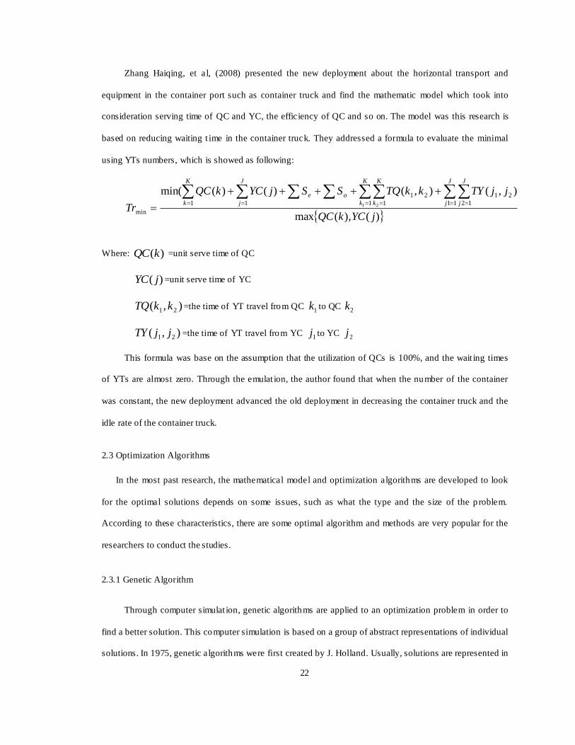
Zhang Haiqing, et al, (2008) presented the new deployment about the horizontal transport and
equipment in the container port such as container truck and find the mathematic model which took into
consideration serving time of QC and YC, the efficiency of QC and so on. The model was this research is
based on reducing waiting t ime in the container truck. They addressed a formula to evaluate the minimal
using YTs numbers, which is showed as following:
)(),(max
),(),()()(min(1 1 1 1 11 12
2121
min1 2
jYCkQC
jjTYkkTQSSjYCkQC
Tr
K
k
J
j
K
k
K
k
J
j
J
j
oe
Where: )(kQC =unit serve time of QC
)( jYC =unit serve time of YC
),( 21 kkTQ =the time of YT travel from QC 1k to QC
2k
),( 21 jjTY =the time of YT travel from YC 1j to YC
2j
This formula was base on the assumption that the utilization of QCs is 100%, and the wait ing times
of YTs are almost zero. Through the emulat ion, the author found that when the number of the container
was constant, the new deployment advanced the old deployment in decreasing the container truck and the
idle rate of the container truck.
2.3 Optimization Algorithms
In the most past research, the mathematical model and optimization algorithms are developed to look
for the optimal solutions depends on some issues, such as what the type and the size of the p roblem.
According to these characteristics, there are some optimal algorithm and methods are very popular for the
researchers to conduct the studies.
2.3.1 Genetic Algorithm
Through computer simulat ion, genetic algorithms are applied to an optimization problem in order to
find a better solution. This computer simulation is based on a group of abstract representations of individual
solutions. In 1975, genetic algorithms were first created by J. Holland. Usually, solutions are represented in
23
binaries of 0s and 1s, but other encodings are also possible. The evolution normally begins from a g roup of
randomly generated individuals and occurs over generations. In each generation, the fitness of every
individual in the group is evaluated; several indiv iduals are selected from the current group depending on
their fitness in order to draw a new population. Th is recombined and mutated population is then used in the
next step of the algorithm. Normally, the search stops when either a maximum number of generations have
been generated or an acceptable fitness level has been obtained for the group. If the search has stopped due
to a maximum number of generations, an acceptable solution may or may not have been reached. Goldberg
(1985) suggested that there are significant advantages if the chromosome can be structured.
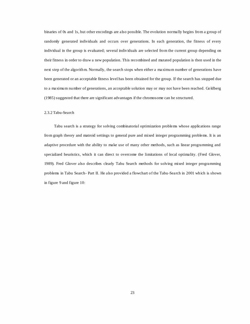
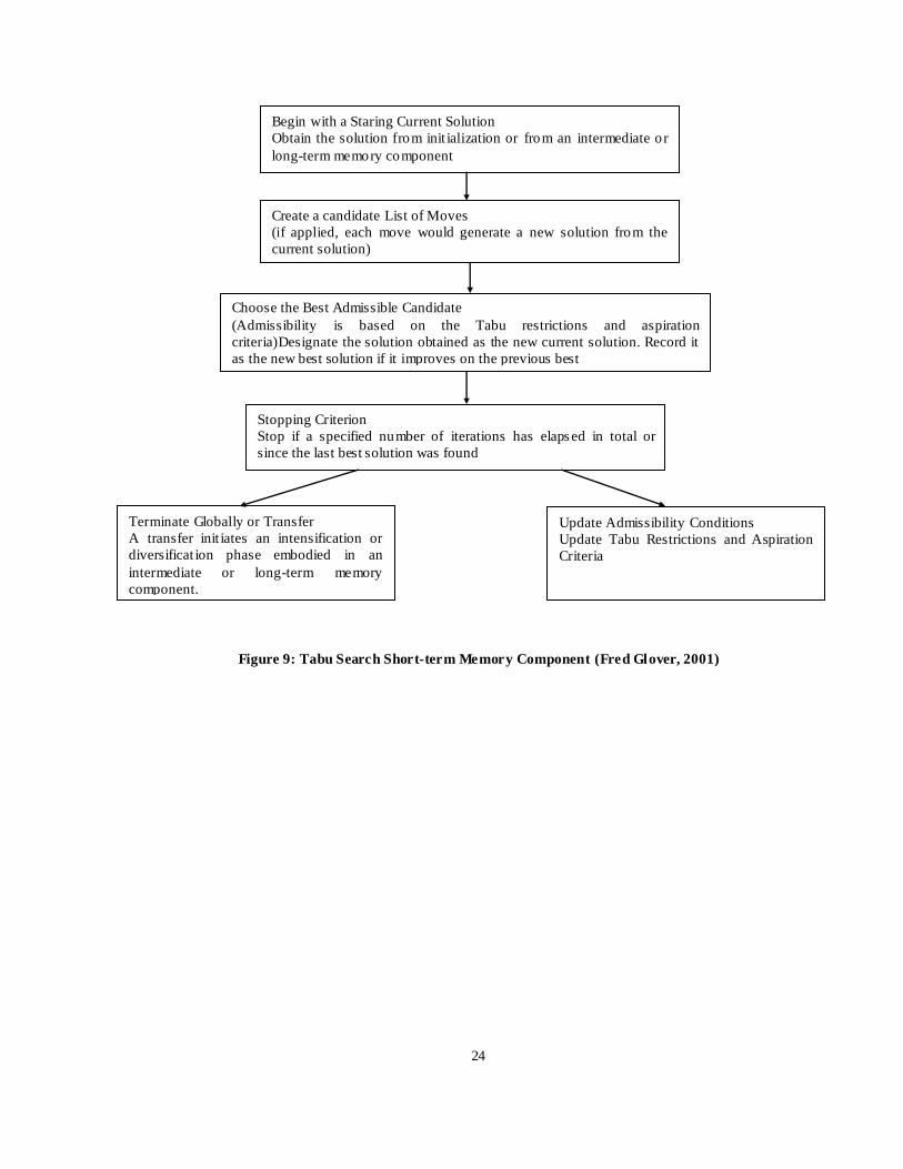
2.3.2 Tabu-Search
Tabu search is a strategy for solving combinatorial optimization problems whose applications range
from graph theory and matroid settings to general pure and mixed integer programming problems. It is an
adaptive procedure with the ability to make use of many other methods, such as linear programming and
specialized heuristics, which it can direct to overcome the limitations of local optimality. (Fred Glover,
1989). Fred Glover also describes clearly Tabu Search methods for solving mixed integer programming
problems in Tabu Search- Part II. He also provided a flowchart o f the Tabu-Search in 2001 which is shown
in figure 9 and figure 10:
24
Figure 9: Tabu Search Short-term Memory Component (Fred Glover, 2001)
Terminate Globally or Transfer
A transfer init iates an intensification or
diversificat ion phase embodied in an
intermediate or long-term memory
component.
Begin with a Staring Current Solution
Obtain the solution from init ialization or from an intermediate o r
long-term memory component
Create a candidate List of Moves
(if applied, each move would generate a new solution from the
current solution)
Choose the Best Admissible Candidate
(Admissibility is based on the Tabu restrictions and aspiration
criteria)Designate the solution obtained as the new current solution. Record it
as the new best solution if it improves on the previous best
Stopping Criterion
Stop if a specified number of iterations has elaps ed in total or
since the last best solution was found
Update Admissibility Conditions
Update Tabu Restrictions and Aspiration
Criteria
25
Figure 10: Selecting the Best Admissible Candidate (Fred Glover, 2001)
2.3.3 Monte Carlo Methods
The Monte Carlo simulation technique has been exp lored since 1940s, where it had applicat ions in
research into nuclear fusion. Monte Carlo methods (or Monte Carlo experiments) are a class of
computational algorithms that depend on repeated random sampling to compute their results. It provides
approximate solutions to a variety of mathemat ical problems by performing statistical sampling
experiments. They can be loosely defined as statistical simulat ion methods, where statistical simulat ion is
defined in quite general terms to be any method that utilizes sequences of random numbers to perform the
simulation. Because of their reliance on repeated computation of random or pseudo-random numbers, these
methods are most suited to calculation by a computer and tend to be used when it is unfeasible or
N
o
N
o
N
o
Y
es
Yes (potential acceptance)
Y
es
Check Aspiration Level
Does move satisfy aspiration
criteria?
Move is Admissible
Designate as best admissible
candidate
Evaluate Each Candidate Move
Does the move yield a higher
evaluation than any other move
found admissible so far (from the
current candidate list)?
Check Tabu Status
Is the candidate Tabu?
Candidate List Check
Is there “good probability” of
better moves left, or should
candidate list be extended?
Make the chosen best admissible
move
Tabu Not Tabu
Admissibility recorded
26
impossible to compute an exact result with a deterministic algorithm. It is also useful for modeling
phenomena with significant uncertainty in inputs.( Jonathan Pengelly,2002)
The technique of Monte Carlo Method means using random numbers in scientific computing. More
precisely, it means using random numbers as a tool to find out the out coming which t is not random. For
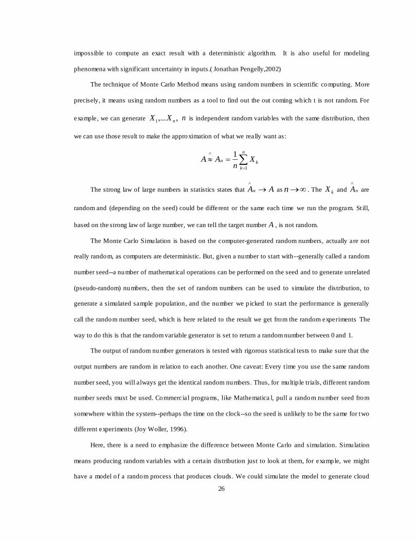
example, we can generate ,,...1 nXX n is independent random variab les with the same distribution, then
we can use those result to make the approximation of what we really want as:
n
k
kn Xn
AA1
1
The strong law of large numbers in statistics states that AAn
as n . The kX and nA
are
random and (depending on the seed) could be different or the same each time we run the program. St ill,
based on the strong law of large number, we can tell the target number A , is not random.
The Monte Carlo Simulation is based on the computer-generated random numbers, actually are not
really random, as computers are deterministic. But, given a number to start with--generally called a random
number seed--a number of mathemat ical operations can be performed on the seed and to generate unrelated
(pseudo-random) numbers, then the set of random numbers can be used to simulate the distribution, to
generate a simulated sample population, and the number we p icked to start the performance is generally
call the random number seed, which is here related to the result we get from the random experiments The
way to do this is that the random variable generator is set to return a random number between 0 and 1.
The output of random number generators is tested with rigorous statistical tests to make sure that the
output numbers are random in relation to each another. One caveat: Every t ime you use the same random
number seed, you will always get the identical random numbers. Thus, for multip le trials, different random
number seeds must be used. Commercial programs, like Mathematica l, pull a random number seed from
somewhere within the system--perhaps the time on the clock--so the seed is unlikely to be the same for two
different experiments (Joy Woller, 1996).
Here, there is a need to emphasize the difference between Monte Carlo and simulation. Simulation
means producing random variab les with a certain distribution just to look at them, for example, we might
have a model o f a random process that produces clouds. We could simulate the model to generate cloud
27
pictures, either out of scientific interest or for computer graphics. As soon as we start asking quantitative
questions about, say, the average size of a cloud or the probability that it will rain, we move from pure
simulation to Monte Carlo .
2.3.4 Brute-Force Search
In computer science, Brute-Force Search, also named exhaustive search, known as generate and test,
is a trivial but very general problem-solving technique that consists of systematically enumerating all
possible candidates for the solution and checking whether each candidate satisfies the problem's statement.
Brute-Force Search is convenient to implement, and will always find a solution if it exists by
checking every solution in the search space until the best global solution has been fou nd. However, its cost
is proportional to the number of candidate solutions, which, in many pract ical problems, tends to grow very
quickly as the size of the problem increases. Therefore, Brute-Force Search is typically used when the
problem size is limited, but very efficiency for small size problem to find the best solution. The method is
defined as the following procedures: is an approximate solution satisfactory or must it be provably optimal?
Heuristics are often used to restrict the search to parts of the state space, thereby sacrificing accuracy for
speed. If a solution must be proven optimal, exhaustive search is used.(Ralph udo gasser,1995).
The general steps for the algorithm are:
Step 1: Align pattern at beginning of test
Step 2: Moving from left to right, compare each character of pattern to the corresponding character in test
until all characters are found to match ( successful search) or a mis match is detected
Step 3 while pattern is not found and the test is not yet exhausted, realign pattern o ne position to the right
and repeat Step 2.
Moreover, a Brute Force solution to a problem involving search for an element with a special
property, usually among combinatorial objects such as permutations, combinations, or subset of a set, the
method is:
Generate a list of all potential solutions to the problem in a systematic manner
Evaluate potential solutions one by one, disqualifying the infeasible ones.
When search ends, announce the solutions found. (The Design & Analysis of Algorithms, 2nd

28
edition, 2007)
Many large problems, for instance integer factorizat ion, traveling salesperson or molecu lar modeling,
can be formulated as search problems. Therefore many researchers focus on problem-independent search
algorithms. Naturally, not all search problems yield to the same algorithms. For those large size search
problems, Branch and Bound Algorithm are popular as another search algorithm in heuristics.
2.3.5 Branch and Bound Algorithm
Solving NP-hard discrete optimization problems to optimality is often an immense job requiring very
efficient algorithms, and the Branch and Bound Algorithm (B&B) is one of the main tools in construction
of these. A B&B algorithm searches the complete space of solutions for a g iven problem to find out the
best solution. However, explicit enumeration is normally an impossible mission due to the exponentially
increasing number of potential solutions. The use of bounds for the function to be optimized combined with
the value of the current best solution enables the algorithm to search parts of the solution space only
implicitly (Jens Clausen, 1999).
For example, it can be assumed that the goal is to find the min imum value of a function f(x), where
the domain of the function is some set S of admissible or candidate solutions (the search space or feasible
region). Note that it is the same to find the maximum value of f(x) by finding the minimum of g(x) = − f(x).
We need two tools in the branch and bound procedure. The first one is a splitting procedure: g iven a
set S of candidates, returns two or more s maller sets ,..., 21 SS which are smaller and the union covers S..
Note that the minimum of f(x) over S is ,...,min 21 vv , where each vi is the min imum of f(x) within Si.
This step is branching, as its recursive application defines a search tree whose nodes are the subsets of S.
Another tool is a procedure that to find out the upper and lower bounds for the min imum value of f(x)
within every g iven subset S. This step is called bounding.

29
3. METHODOLOGY AND MODEL DEVELOPMENT
3.1 Preliminary
For most container terminals, there are mainly three types of equipment involved in the operations of
the containers, which are Quay Cranes (QCs) worked in the berth, Yard Cranes (YCs) worked in the yard,
and Yard Trailers (YTs) worked to transfer containers between berths and yards . Because of the complexity
of the scheduling of the YTs in the container terminal, how to dispatch and assign these YTs reasonably is
the most important. The rules of dispatching this equipment are various. Generally, trad itional operation
and dynamic operation are widely used based on the container volume in the container terminal within
different periods.
3.1.1 Traditional Operat ion
As the traditional method (static operation), the port dispatchers deploy the mechanical equip ment
according to the storage plan of vessels, the number of containers , and the yard slots allocation when the
vessel is mooring in the berth. This means that when the vessel arrives, it should be determined whether it
needs to be loaded or unloaded first. Then port dispatchers will deploy corresponding Quay Cranes (QCs)
depending on the container volume. Based on the number of the QCs, each crane is equipped with 3-4 Yard
Trailers (YTs), which means that the assigned YTs are fixed to on ly a specific QC, and each YT operates a
clockwise d irection along the transport route. The QCs are working until the vessel leaves the berth. In the
process of loading and unloading, QCs, YTs, and YCs are formed into a fixed-line, shown in figure 11 (Liu,
2009).The advantage of this method is that it is easy to operate. However, it cannot meet the requirements
in the case that there is a large volume of containers that need to be unloaded and loaded; it always causes
gap time, which decreases the productivity. The disequilibrium of d ifferent working lines (QCs) may occur.
For instance, some QCs may face a shortage of YTs, which probably decrease the entire operation‟s
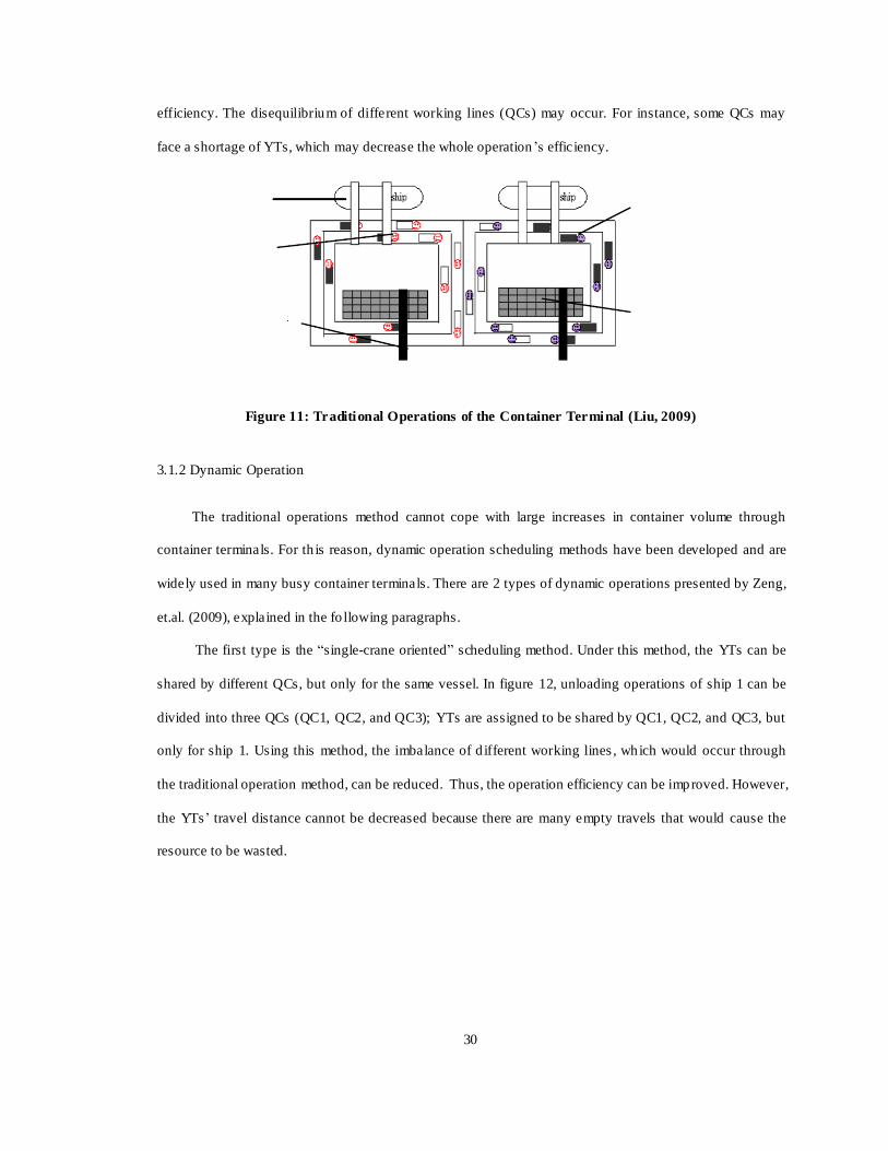
30
efficiency. The disequilibrium of different working lines (QCs) may occur. For instance, some QCs may
face a shortage of YTs, which may decrease the whole operation ‟s efficiency.
Figure 11: Traditional Operations of the Container Terminal (Liu, 2009)
3.1.2 Dynamic Operation
The traditional operations method cannot cope with large increases in container volume through
container terminals. For th is reason, dynamic operation scheduling methods have been developed and are
widely used in many busy container terminals. There are 2 types of dynamic operations presented by Zeng,
et.al. (2009), explained in the fo llowing paragraphs.
The first type is the “single-crane oriented” scheduling method. Under this method, the YTs can be
shared by different QCs, but only for the same vessel. In figure 12, unloading operations of ship 1 can be
divided into three QCs (QC1, QC2, and QC3); YTs are assigned to be shared by QC1, QC2, and QC3, but
only for ship 1. Using this method, the imbalance of d ifferent working lines , which would occur through
the traditional operation method, can be reduced. Thus, the operation efficiency can be improved. However,
the YTs‟ travel distance cannot be decreased because there are many empty travels that would cause the
resource to be wasted.
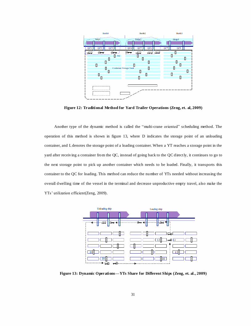
31
Figure 12: Traditional Method for Yard Trailer Operations (Zeng, et. al, 2009)
Another type of the dynamic method is called the “multi-crane oriented” scheduling method. The
operation of this method is shown in figure 13, where D indicates the storage point of an unloading
container, and L denotes the storage point of a loading container. When a YT reaches a storage point in the
yard after receiv ing a container from the QC, instead of going back to the QC d irect ly, it continues to go to
the next storage point to pick up another container which needs to be loaded. Finally, it transports this
container to the QC for loading. Th is method can reduce the number of YTs needed without increasing the
overall dwelling time of the vessel in the terminal and decrease unproductive empty travel, also make the
YTs‟ utilization efficient(Zeng, 2009).
Figure 13: Dynamic Operations—YTs Share for Different Ships (Zeng, et. al., 2009)
32
In this study, the operations based on the “mult i-crane oriented” scheduling method will be
simulated. The model focuses on the deployment of the YTs as well as considers the serving time of
QCs and YCs.
3.2 The Basic Idea of Modeling
According to practical experience, the mooring cost of the vessels is usually higher than the cost of
using the YTs. Therefore in this study, the first principle is that the mooring time of the unloading vessel
should be as short as possible. For this purpose, it is necessary to ensure that there are enough YTs for the
unloading operations to run smoothly without gap time.
The time duration for one YT to finish a cycle of unloading and loading is random, and it depends
equally on the distance of the path the YT travels as well as on the unloading and loading position the YT
chooses. The intent of this study is to find all the different paths and to strategically pick the longest one
amongst them as the decision basis. Then the distance that a random YT travels in its cycle will be no
longer than this; thus, the additional YTs will spend no more t ime than this for any other travels . A natural
result is that if the total number of the YTs is enough for this maximal time duration situation, then it will
be enough for any other, so this strategy serves the first princip le loyally --- reducing the mooring cost of
the vessels.
However, it somewhat requires a considerably large number of YTs, which will cause queuing at
those operating terminals and increase the cost of vehicles (YTs). So, under the first principle, the second
principle is to find an appropriate total number of YTs that can quantitatively minimize the total cost ---
both the vessels mooring cost and the YTs working cost.
3.3 Problem Assumptions and Analysis
Different from the most literatures of the past, this study, based on Zhang‟s paper in 2008, tries to use
the minimal wait ing time of unloading vessel as the basis for estimation, and then calculates the number of
YTs which are necessary for it, in order to make the operations system run. It turns a series of individual
operations for YTs, which include loading, unloading and ground operations, into one integrated
deployment schedule, in which YTs can be used in all these tasks.

33
This study will help YTs to achieve the fully utilization. YTs work on the way between QCs and YCs
and other empty YTs can be added dynamically to the operating line at anytime. It can reduce YTs ‟ waiting
time and fully use cranes, in order to reach the minimal number of YTs in use in order to make them
achieve efficiency. Additionally, the costs of mooring the unloading vessel in the berth are considered as
well as the costs of the YTs. They will be acted as elements of the objective function.
As the studied problem is concerning an integrated handling system of the container termina l, the
combination of operations is shown in the figure 14. Before the development of the model, assumptions
would be supposed:
(1) Suppose there are two vessels, Vessel1 and Vessel 2 for unloading and loading respectively; the
operations of the two vessels are scheduled simultaneously:
The ideal model is developed supposing the container volume of both the unloading and loading
vessels are balanced, in order to make the YTs can be used in a fu ll circle;
These containers are operated from on ly one side of the vessels;
The unit time of QC operations are constant;
Because there is a cost for being moored along the berth of unloading vessels, the gap time of two
unloading operations needs to be decreased as much as possible, try ing to best make the operations of
unloading continuous. So, to be most efficient, at the point S there should be at least one YT every unit
time of QC operation. (Assume every operation just can deal with one container).
(2) There are two storage yards in this model.
d
1 S
1
S
2
S D
A
r
i r
j
d
2 B
Vessel1 1 Vessel2
Figure 14: One Circle of YT Travel Route
34
Left yard, called S1, is for loading containers which are from the unloading vessel (vessel 1 in the
figure) to be stored temporally. The rule is that the containers can be stored at any empty slot
temporarily, so in this model, the point in this area will be selected randomly;
The other storage yard, S2, is the area where the containers are picked to be loaded to the loading
vessel (vessel 2 in the figure), according the description of the yard in the introduction of this
study: always are stacked based on certain ru les or p lans in this yard before loading to the vessel,
in this study, the details of the rule will not be developed. To consider this issue, the loading
containers will be separated into several groups, and we give some weight value to define the
different groups of containers, some of which are defined with the larger number, are first served.
In the following model, there are 4 groups of containers which are valued with 4,3,2,1 and will be
operated as the certain rule: 4-3-2-1;
Four containers can be stored in one point.
The unit times of YC operations in the yards are constant, and assume the YCs are enough that
when YT reaches the points, the YC is ready to connect the job.
(3) This study focuses on the finding the proper number of YTs, so the main object is the YT. For whole
operations of the YT.
The job of each YT worked for both unloading a container and loading a container can be
described as a circle: it starts from point S at the unloading vessel, then it p icks up a container
from a QC worked from the unloading vessel to store it in the area S1, and then goes to area S2 to
pick up another container to load it to the loading vessel. This operations assignment of YTs can
reduce the empty ride, which is more efficient.
As the points in the yards are random, the travel distances of the circles are random, and the travel
time of every circle is also random.
The travel distance of an YT for one circle is shown in the figure 14. The whole distance of one
circle (for each YT) can be separated into 6 sections, which are d1, d2, d3, d4, d5, d6. d1, d2, d3 are
constant because the position of vessels and yards are fixed, and d4, d5, d6 are variables as the
storage points are unknown. It can be expressed through coordinates, however, within the path

35
(A-Pa-Pb-B), it is not a straight line connecting every 2 points in the yards, the real distance
between these 2 points are also not the straight line Euclid distance. 1-norm 1
rd will be
expressed as the real distance.
(4) Because of the randomness of the total time of YTs, the number of the YTs which need to be
replenished is also random, which leads to the cost for yard trailers in use is the ext raneous variable.
We assume that the cost for the use of yard trailer is expressed as a increasing function, )(kVC , while
the cost for mooring the berth of unloading vessel is expressed as an decreasing function, with k is the
number of YTs, because the more YTs that are used, the more cost from this part. However, the more
YTs availab le for use, the less time needed for operations, so mooring the berth cost will be less.
However, as the variable )(kMC approaches a certain value it will become constant from the point of
the proper number of YTs available, because an increase in the number of YTs available past this point
will cause no reduction in total operations time. Also, after combination of these two kinds of cost,
there is a balance point (H), shown in the figure 15.
Figure 15: The Relationship between the Cost Function and the Number of YTs
v
0
VC(k)
MC(k)
H
v0

36
3.4 Modeling
Based on these assumptions, this problem will be developed as a mathematical model with constraints
and objective function, as well as some issues that can be also described as math formulas, which are used
to replicate and define the simulation.
3.4.1 Notations and Variables
Firstly, the data sets, variables and parameters used in the formulation are defined before development
of the mathematical model.
Data
R : Total number of distance sections, Rr
N : Total number of containers for unloading,
N : Total number of containers for loading, Ncc ',
A : Store point sets in the storage area for loading containers from unloading vessel (which is left
area in the figure 14), Aa
B : Store points set in the storage are o f p icking up containers for loading vessel (which is right area
in the figure 14), Bb
I : Total number of YTs
L : Total cycles done by all YTs
Indices:
r : Index for different section travel distance, 1,...,r R .
a : Index for the points in the area S1 which is for storage, 1,...,a A .
b : Index for the points in the area S2 Which is for p icking up, 1,...,b B .
c : Index for the containers which are need to be loaded,
1,...,c N
i : Index for different YTs, 1,...,i I .
l : Index for different cycles done by each YT, 1,...,l L .
Variables:
k : The number of YTs in use
aP :
The random position in the yard S1 fo r storage which is available
1
( , )a a a
P x y S
bP :
The random position in the yard for loading to the vessel which is availab le
2),( SyxP bbb

37
( )MC k : The cost for mooring in the berth of unloading vessel with k YTs.
( )VC k : The cost for YTs fee with k YTs.
rd : The travel distance of r
th section, 4r
ild :
The distance of the pth
cycle of the ith
YT
ilo :
The value of the loading containers
ilt : The working time of the p
th cycle of the i
th YT
1,( , )
0,a a ax y
If the point Pa has been already occupied
Otherwise
1,( , )
0,b b bx y
If the point Pb has the containers needed to be loaded
Otherwise
Parameters:
0Qut : The time of unit operation of unloading with a QC (min)
0Qlt :
The time of unit operation of loading with a QC (min)
1d : The distance between unloading vessel and yard S1for storage.(S → A)(mile)
2d : The distance between yard for loading and loading vessel(B → D)(mile)
3d : The distance between the two vessels(D → S) (mile)
0Y ut : The time of unit operations for YC in the yard for storage (min)
0Y lt : The time of unit operations for YC in the yard for loading to the vessel (min)
v : The speed of the trucks (meter/min)
0MC : The unit cost of mooring in the berth of unloading vessel ($/min)
0V C : The unit cost of YTs fee ($/min*per)
1 2 1 2, , ,m m n n :
The length and width of the two storage areas(S1,S2)
3.4.2 Mathemat ical Analysis and Objective Function
(1) According to the first principle, that the mooring time of the unloading vessel should be as short as
possible, enough numbers of YTs needs to be assigned at the unloading point to make the system
operation run without any delay. So, from this point, there should be at least one YT every unit time of
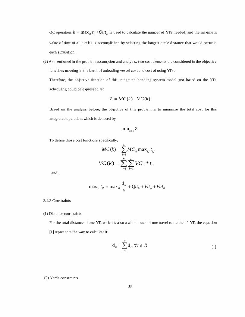
38
QC operation. oilil Quttk /max is used to calculate the number of YTs needed, and the maximum
value of time of all circles is accomplished by selecting the longest circle distance that would occur in
each simulat ion.
(2) As mentioned in the problem assumption and analysis, two cost elements are considered in the objective
function: mooring in the berth of unloading vessel cost and cost of using YTs.
Therefore, the objective function of this integrated handling system model just based on the YTs
scheduling could be expressed as:
( ) ( )Z MC k VC k
Based on the analysis before, the objective of this problem is to minimize the total cost for this
integrated operation, which is denoted by
1min
kZ
To define those cost functions specifically,
0 , ,
1
( ) maxL
i l i ll
MC k MC t
k
i
L
l
iltVCkVC1 1
0 *)(
and,
00maxmax VutVltQltv
dt o
il
ililil
3.4.3 Constraints
(1) Distance constraints
For the total d istance of one YT, which is also a whole track of one travel route the ith
YT, the equation
[1] represents the way to calculate it:
RrdR
r
r
,d1
il
(2) Yards constraints
[1]

39
The equations [2] and [5] show that what the ranges of coordinates are with in, in order to define the
size of yards.
2
1
2
1
0
0
0
0
my
ny
mx
mx
b
a
b
a
(3) Container and loading sequence constraints
To simplify the model, also in order to make YTs efficient, we match each inbound container to each
outbound container, means the volume of both unloading and loading are balance, the equation [6]
restrict it:
NN
As stated before, there should be a rule for the loading sequence of containers to vessels from the yard.
To consider this point and to also to help the model to be developed easier, we define containers into
the four groups with different values, and the sequence of picking up containers to be loaded based on
said values. Some of the containers with the larger number will be loaded first. As in the equation [7],
the value of the container 1c , which is the next loading container immediately follows container c ,
will be loaded in the loading vessel and cannot be exceed by the value of the last container of which is
just loaded. It should be under the certain rule in which the s maller value of containers cannot skip the
containers with larger value.
10
c co o
3.5 Some Discussion
The following issues need to be discussed:
(1) When k increases, ( )MC k decreases because making the operations system keep running,
especially at the unloading point, is the main purpose. however, )(kMC , this value will approaching a
certain value with the increase of the number of YTs, because when the YTs are enough to be served
for total containers, the operations time will be certain.
[4]
[3]
[2]
[5]
[6]
[7]
40
(2) When k increases, ( )VC k increases. The queuing is pretty likely to happen because our strategy is
to choose k based on the longest path always. But in real situation every YT will arrive at the
unloading terminal for a shorter time, and stocking queuing happens. Straight forward to calculate the
cost of queuing in this case is very complicated, so this study tries to look for the relat ionship between
the costs and k through the numerical simulat ion method.
(3) Cost calculation firstly depends on two main parameters: unit vessel cost 0
MC and unit vehicle cost
0V C , the ratio between them d irectly determines how much vehicle costs we should sacrifice for
vessel cost. And, there are another several parameters affect the travel t ime of each circle and the
queuing condition, unloading, such as the load of Vessel 1, which can be simply represented as total
unloading number of containers divided by the number of QCs, as well as the unit operations time of
every kind of cranes.
41
4. SIMULATION AND RESULT ANALYSIS
4.1 Simulation Idea and Algorithm
The purpose of this model is to look through the simulat ion for the best number of YTs with the
lowest cost, so the object of the simulat ion is YT. The total time of one cycle of the YT‟s travel route
includes the traveling time of all six sections and the YCs‟ unit operations in those two yards , as well as
one loading operation of the QC, which is formulated in the following equation:
0 0 0
il
il
dt Y ut Y lt Qlt
v
Here, the equation overlooks the unloading operation time of the QC from the unloading vessel because the
cost of mooring in the berth in the objective function focuses on this unloadin g vessel. The operations of
YTs are optimized for th is vessel.
Furthermore, according to the total time per cycle, the number of YTs , which needs to be used to meet
the volume requirement without any waiting time of QCs for this current condition, can be calculated with
the following. The value calculated through this equation can reach zero gap time each cycle to make the
operations connective:
IiLlQuttk ilil ,,/ 0
Because the time of each cycle of YTs varies from reaching different storage points, there should be a
maximum value ,
maxi l il
t among all possible outcomes. The unloading operations will never stop if in
,max
i l ilt YTs are equipped because during the cycle of any YT, there are always enough other YTs to
unload containers from Vessel 1.
Therefore, due to the length of the yards and the technical limitat ions, the entire system is simulated
for selected values of k in various given circumstances. Also, based on the simulation results , the value of
42
k in certain circumstances is approximately concluded, and the rough relationship between k and the most
important given parameters will be considered.
In this study, two methods are employed to achieve the simulation of the operations . The Monte Carlo
method is a computational method to approach the optimal solutions by probability statistics. First, in this
model, the simple technique of this method is proposed to generate pseudo random numbers for the points
in the storage yard to represent the real storage position for the containers in the simulation. The yards will
be expressed as matrixes, and each storage point will be denoted as 0 or 1 to define the condition of every
specific slot. Because the number of containers which always are provided before starting the operations in
the real cases, so the operations need to be served can be known before, the range of YTs usage is defined
to restrict the number of YTs in order to avoid worthless. That means there is a range of how many YTs
determined with each volume of containers workload. So, in this study, the different cases with d ifferent
number YTs will be simulated as experiments, so based on those cases provided at the beginning, Brute-
force Method will be combined into algorithm to list all the situations results, and compare them. It will be
conducted as the major circle of this simulation. Particularly, the steps of the developed algorithm for this
specific problem are expressed in the following, and the logic flowing chart is shown in figure 16.

43
Figure 16: Flow Chart of the Algorithm
YES
(1) Assign the initial waiting
time value to YTs
(4) Generate the coordinates of
r1, r2 by pseudo-random
numbers to be represented
as the storage points
(3) Start Simulation, j=1
(5) Calcu late the whole
distance of one route and
the time of it t
(6) Sort the group of t
Is the number of
operations of YTs is
equal to the
operations times of
one QC?
(7) The s mall circu lation of
one case is finished; the
total time of all operations
can be obtained
(8) Calcu late the value of cost
(9)Simulat ion Over, Sort the
group of total cost numbers,
determine the best number
of YTs
Is the number of
circulat ion (j) equal
to the cases with
different number of
YTs?
NO
NO
j=j+1
(2) Match each outbound
container to inbound
container
YES
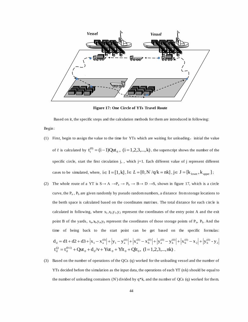
44
Based on it, the specific steps and the calculation methods for them are introduced in following:
Begin :
(1) First, begin to assign the value to the time for YTs which are waiting for unloading,init ial the value
of t is calcu lated by k)1,2,3,...,(i , Qut)1i(t 0
(0)
i ,the superscript shows the number of the
specific circle, start the first circulation j, , which j=1. Each different value of j represent different
cases to be simulated, where, k][1,Ii , nk]/q/kN[0,l - L , ]k,[kJj upperlower ;
(2) The whole route of a YT is S→ A →Pa → Pb → B→ D →S, shown in figure 17, which is a circle
curve, the Pa , Pb are given randomly by pseudo random numbers, a d istance from storage locations to
the berth space is calculated based on the coordinates matrixes. The total d istance for each circle is
calculated in following, where x1 ,x2,y1,y2 represent the coordinates of the entry point A and the exit
point B of the yards, xa,xb,ya,yb represent the coordinates of those storage points of Pa, Pb. And the
time of being back to the start point can be get based on the specific formulas:
2
(il)
b2
(il)
b
(il)
b
(il)
a
(il)
b
(il)
a
(il)
a1
(il)
a1il y-yxxyyxxyyxxd3d2d1d
nk)1,2,3,...,(l ,QltYltYut/vdQuttt 000il0
1)-(0
il
(j)
il .
(3) Based on the number of operations of the QCs (q) worked for the unloading vessel and the number of
YTs decided before the simulat ion as the input data, the operations of each YT (nk) should be equal to
the number of unloading containers (N-) d ivided by q*k, and the nu mber of QCs (q) worked for them.
d
1 S
1
S
2
S D
A
r
a r
b
d
2 B
Vessel
1
Vessel
1
d
1
d
3
d
4
d
5
d
6
Figure 17: One Circle of YTs Travel Route
tra

45
Sort k
1i
(j)
ilt,which is the set of t value of YT after one loop, where then obtain a new wait ing time
k
1i
)(j'
ilt。Compare the time value of every YT, If o
)(j'
il
)(j'
1)l(i Qutt-t , it means that the YTs are
enough for 0 delay, meanwhile , o
)(j'
il
)(j'
1)l(i Quttt ,o
(*)
i
(*)
1i Quttt . If
o
)(j'
il
)(j'
1)l(i Qutt-t , it means that the backing YT cannot connect with last truck with no gap, the
trucks is not enough to obtain 0 delay, so there is the cost for delay in this case. In this case,
)(j'
1)l(i
)(j'
1)l(i tt . As a result, the total time for the case of k YTs after one circle, also can be
represented as the initial time of the next circle, can be obtained, that
is )1,2,3,...kink,1,2,3,...,(l , t t )(j'
il
(j)
1)i(l .
(4) If the number of YTs operations is less than the operations times of one QC, repeat 1-3 steps. If not,
go to step 5.
(5) After the circulation done, the total time of each YT it multiple the unit fee , to get the utilization cost
of k YT in one Quay Crane, it is )(kVC . In all YTs, the biggest value among the set of it is the total
operations time of unloading operations for the unloading vessel, also can be treated as the mooring
time in the berth of unloading vessel, so there is a cost for it, it is )(kMC .
(6) Consider the number of Quay Cranes (q), total YTs are kq * ,cost for utilization is )(* kVCq ,
cost for delay is still )(kMC ,total is )()(* kMCkVCq 。
(7) Simulate different cases with different number o f using YTs, if the number of circulat ions cannot
cover all cases provided based on the number of YTs for use, go back to the first step, with
j=j+1,otherwise, stop the all circulat ion.
(8) Listing all of the results from those circulat ions, the best feasible number of YTs with the minimal
total cost can be obtained from comparison.
(9) Repeat 1-8 steps by multip le times, the statistical result can be approached.
End

46
4.2. Computation
According to the reality, the value of all parameters can be set up, and collecting the probabilities of
all cases through computer simulat ion, then, the best value with min imal cost can be obtained in the certain
condition.
4.2.1. Test Design and Results
Some tests for models will be conducted. Take a typical container as an example: there are two
vessels in the berths at a certain moment, and they need to be unloaded and loaded simultaneously. The
total number of containers that are needed to be unloaded from the unloading vessel is 2400. To balance the
transportation of YTs, the loading containers volume is also 2400.The containers considered in this model
are Twenty-foot Equivalent Units (TEU: 20ft*8ft*8.5ft). Moreover, the distance between the unloading
vessel and the yard S1 is 1 km, the distance between the other yard S2 and the loading vessel is 1km, and the
distance between these two vessels is 1km. The unit time of the QCs are 2 minutes per container, both for
unloading and loading operations, and the unit t ime of unloading operations of the YCs is 1.5 minutes per
container. However, the unit time of loading operations of the YCs is 1 minute per containers. The velocity
of YTs is 20 kilometers/hour. The unit cost for using YTs is assumed as $0.2 per minute, and the unit cost
for mooring in the berth of the unloading vessel is $30 per minute by assumptions.
The slot condition is generated randomly by matrixes through MATLAB. These specific two yards in
the model, are represented by the coordinate matrixes in two dimensions, in order to calculate the distances.
We consider four layers is allowed in the yards which means there are 4 containers can be store at every
specific storage point. In programming, another two matrix composed by 0-4 with the same size of
coordinate matrixes are generated, each coordinate can match a number between 1 to 4 to express how
many container are already in this point. For the yard where the loading containers are stored, to consider
the loading sequence of these containers to the vessel, we separate them in to four groups, with d ifferent
number to represent the situation of the containers in each groups: 4,3,2,1: the containers graded with 4
should be loaded first, then 3,2,1. The containers with the smaller numbers cannot be loaded in the front, if
there are still some containers with the numbers larger left. In real world, the loading rules designed based
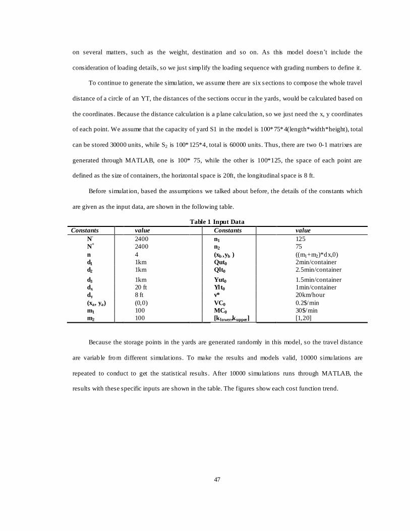
47
on several matters, such as the weight, destination and so on. As this model doesn‟t include the
consideration of loading details, so we just simplify the loading sequence with grading numbers to define it.
To continue to generate the simulation, we assume there are six s ections to compose the whole travel
distance of a circle of an YT, the distances of the sections occur in the yards, would be calculated based on
the coordinates. Because the distance calculation is a p lane calcu lation, so we just need the x, y coordinates
of each point. We assume that the capacity of yard S1 in the model is 100*75*4(length*width*height), total
can be stored 30000 units , while S2 is 100*125*4, total is 60000 units. Thus, there are two 0-1 matrixes are
generated through MATLAB, one is 100* 75, while the other is 100*125, the space of each point are
defined as the size of containers, the horizontal space is 20ft, the longitudinal space is 8 ft.
Before simulat ion, based the assumptions we talked about before, the details of the constants which
are given as the input data, are shown in the following table.
Table 1 Input Data
Constants value Constants value
N- 2400 n1 125
N+ 2400 n2 75
n 4 (xb ,yb ) ((m1+m2)*dx,0)
d1 1km Qut0 2min/container
d2 1km Qlt0 2.5min/container
d3 1km Yut0 1.5min/container
dx 20 ft Ylt0 1min/container
dy 8 ft v* 20km/hour
(xa, ya) (0,0) VC0 0.2$/min
m1 100 MC0 30$/min
m2 100 [k lower,kupper] [1,20]
Because the storage points in the yards are generated randomly in this model, so the travel distance
are variab le from different simulat ions. To make the results and models valid, 10000 simulations are
repeated to conduct to get the statistical results . After 10000 simulations runs through MATLAB, the
results with these specific inputs are shown in the table. The figures show each cost function trend.
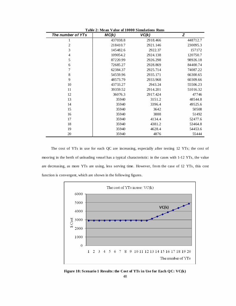
48
Table 2: Mean Value of 10000 Simulations Runs
The number of YTs MC(k) VC(k) Z
1 437038.8 2918.466 448712.7
2 218410.7 2921.146 230095.3
3 145482.6 2922.37 157172
4 109054.2 2924.138 120750.7
5 87220.99 2926.298 98926.18
6 72685.27 2928.869 84400.74
7 62384.37 2925.714 74087.22
8 54559.96 2935.171 66300.65
9 48573.79 2933.968 60309.66
10 43733.27 2943.24 55506.23
11 39359.52 2914.201 51016.32
12 36076.3 2917.424 47746
13 35940 3151.2 48544.8
14 35940 3396.4 49525.6
15 35940 3642 50508
16 35940 3888 51492
17 35940 4134.4 52477.6
18 35940 4381.2 53464.8
19 35940 4628.4 54453.6
20 35940 4876 55444
The cost of YTs in use for each QC are increasing, especially after testing 12 YTs; the cost of
mooring in the berth of unloading vessel has a typical characteristic: in the cases with 1-12 YTs, the value
are decreasing, as more YTs are using, less serving time. However, from the case of 12 YTs, this cost
function is convergent, which are shown in the following figures.
Figure 18: Scenario 1 Results: the Cost of YTs in Use for Each QC: VC(k)
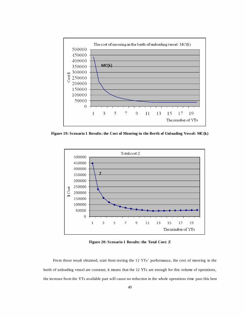
49
Figure 19: Scenario 1 Results: the Cost of Mooring in the Berth of Unloading Vessel: MC(k)
Figure 20: Scenario 1 Results: the Total Cost: Z
From those result obtained, start from testing the 12 YTs‟ performance, the cost of mooring in the
berth of unloading vessel are constant, it means that the 12 YTs are enough for this volume of operations,
the increase from the YTs available part will cause no reduction in the whole operations time past this best

50
number of YTs point. Also, there is no linear relat ionship between the costs of YTs in use and YTs‟
quantity. This cost based on not only the number of YTs, but also the working t ime of those YTs. So, from
the point of 12 YTs, the cost of YTs in use for each QC increases significantly, as there is no reduction in
YTs‟ working time. Therefore, in case of 12 YTs those are for usage, the minimal cost can be reached in
this condition. So, totally there are 4 QCs served for unloading vessel, totally 36 YTs are needed, and the
total cost is 2906.4*4+35940=47565.6.
To test how the container storage configuration affect the results, 10 simulat ions results are selected
randomly to be compared among them. The total cost function curves are shown in the following. From
those results, we can see the different kinds of cost are variable in the tests of 1-11 YTs, and the 12 YTs are
still the proper number of YTs in usage, the total cost are same from 12 YTs to 20 YTs, this characteristic
is same as we exp lained before that 12 YTs can be served for all of the operations with no gap, and from
that point, the total time of mooring in the berth of unloading vessel are constant, the spare YTs cannot
provide any benefit in reduction time, so only produce the costs of YTs in use, which are become a constant
here. The figure 21 shows that before the best number of YTs is reached, there are very small d ifferences in
cost between 10 simulat ions . After this point, cost is the same. So, the configuration of the containers has
negligible effect on the cost.
Figure 21: Ten Random Simulation Results

51
4.2.2. Other Numerical Tests and Analysis
Furthermore, numerical tests will be conducted to examine the validity of the simulation performance.
According to the description in part 3.4, these tests are in order to find the relationship between some main
parameters and the number of YTs. Cost calculat ion first depends on two main parameters: unit vessel cost
0MC and unit vehicle cost 0VC . The ratio between them d irectly determines how much vehicle cost we
should sacrifice for vessel cost. And, there are another several parameters that affect the travel time of each
circle. The queuing condition, the load of Vessel 1 unloading, can be simply represented as the total
unloading of the number of containers divided by the number of QCs, as well as the unit operation ‟s time
of every kind of cranes.
(1) Change in the ratio of the unit cost of unloading vessel moor and the unit cost of vehicle.
The unit cost of mooring of vessels and the unit cost of YTs vary depending on many factors, such as
the port situation, the size and owner of the terminals, and the volume of the operations, if there are some
leases between the port authority and the vessel companies. However, according to the actual situation,
there should be a range that these two cost values can fluctuate within. 0MC can fluctuate within [5, 30],
while 0VC can be different within [0.2,1]. Based on them, combining these two values randomly, 10 tests
are conducted, and the results are shown in the following table:
Table 3: The Results with Different Unit Cost
VC0-MC0 The number of YTs MC(k) VC(k) Z
0.7-23 12 27661 10211.5 68507
0.3-15 12 18038.4 4376.20 35543.20
0.6-15 12 18039.8 8753.41 53053.44
1-5 12 6013.05 14587.67 64363.72
0.8-9 13 17970 9453.60 55784.40
We can see the best number of YTs in use is also approximately 12. Therefore, the best number of YTs in
use is not sensitive to the cost change within those ranges.
(2) Change the ratio of the unloading volume and the number of QCs
In this part, based on most of the input data from the previous test design part, with the same unit
operation time of QCs, the same velocity of YTs, and the same size and definition of both yards, only the
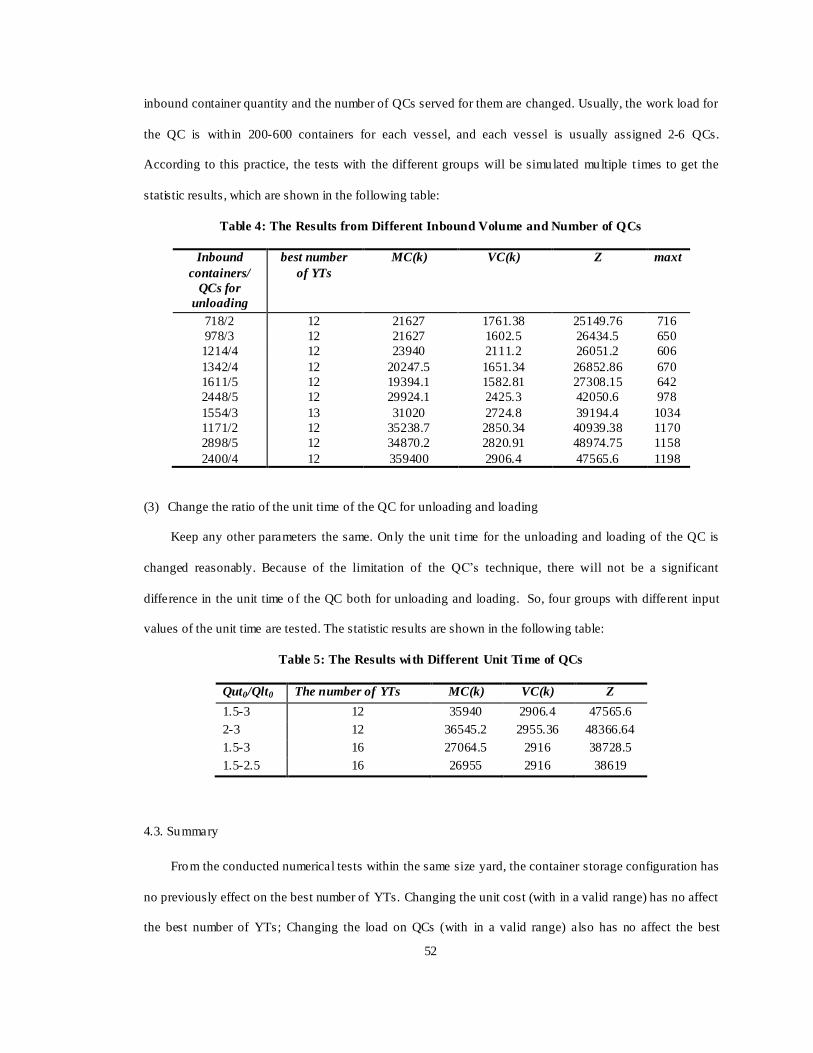
52
inbound container quantity and the number of QCs served for them are changed. Usually, the work load for
the QC is with in 200-600 containers for each vessel, and each vessel is usually assigned 2-6 QCs.
According to this practice, the tests with the different groups will be simulated multiple t imes to get the
statistic results, which are shown in the following table:
Table 4: The Results from Different Inbound Volume and Number of QCs
Inbound
containers/
QCs for
unloading
best number
of YTs
MC(k) VC(k) Z maxt
718/2 12 21627 1761.38 25149.76 716
978/3 12 21627 1602.5 26434.5 650
1214/4 12 23940 2111.2 26051.2 606
1342/4 12 20247.5 1651.34 26852.86 670
1611/5 12 19394.1 1582.81 27308.15 642
2448/5 12 29924.1 2425.3 42050.6 978
1554/3 13 31020 2724.8 39194.4 1034
1171/2 12 35238.7 2850.34 40939.38 1170
2898/5 12 34870.2 2820.91 48974.75 1158
2400/4 12 359400 2906.4 47565.6 1198
(3) Change the ratio of the unit time of the QC for unloading and loading
Keep any other parameters the same. Only the unit t ime for the unloading and loading of the QC is
changed reasonably. Because of the limitation of the QC‟s technique, there will not be a significant
difference in the unit time of the QC both for unloading and loading. So, four groups with different input
values of the unit time are tested. The statistic results are shown in the following table:
Table 5: The Results with Different Unit Time of QCs
Qut0/Qlt0 The number of YTs MC(k) VC(k) Z
1.5-3 12 35940 2906.4 47565.6
2-3 12 36545.2 2955.36 48366.64
1.5-3 16 27064.5 2916 38728.5
1.5-2.5 16 26955 2916 38619
4.3. Summary
From the conducted numerical tests within the same size yard, the container storage configuration has
no previously effect on the best number of YTs. Changing the unit cost (with in a valid range) has no affect
the best number of YTs; Changing the load on QCs (with in a valid range) also has no affect the best
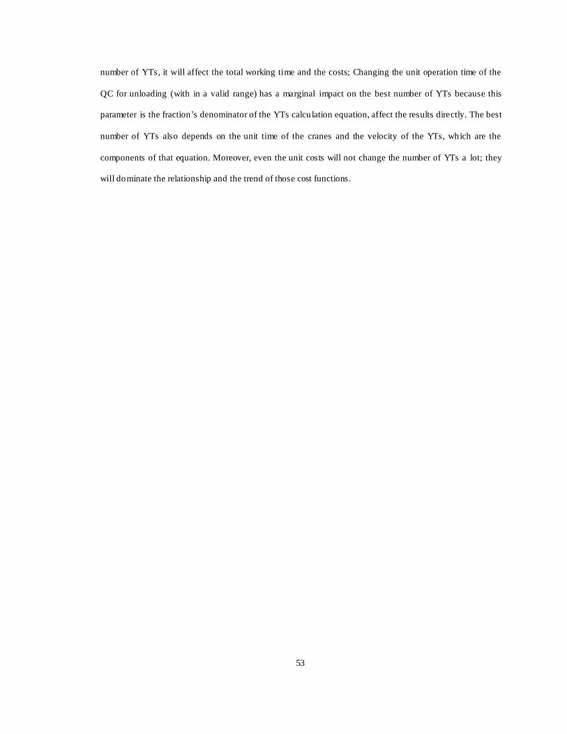
53
number of YTs, it will affect the total working time and the costs; Changing the unit operation time of the
QC for unloading (with in a valid range) has a marginal impact on the best number of YTs because this
parameter is the fraction‟s denominator of the YTs calcu lation equation, affect the results directly. The best
number of YTs also depends on the unit time of the cranes and the velocity of the YTs, which are the
components of that equation. Moreover, even the unit costs will not change the number of YTs a lot; they
will dominate the relationship and the trend of those cost functions.
54
5. CONCLUSION
This study simulates the operations procedures using dynamic YTs operation‟s method. It seeks to
produce a simulat ion method to understand how this method works and find and evaluate the best feasible
solution that considers both minimal cost and increased efficiency of operations for the proper number of
Yard Trailers (YTs) at the container terminal. Currently, there has been an exponential increase in container
volume shipment within intermodal transportation systems. Container terminals as part of the global port
system represent important hubs within this intermodal transportation system. Thus, the need to improve
the operational efficiency is the most important issue for container terminals from an economic standpoint
and that is why, during recent years, much emphasis has been placed on optimizat ion and simulation of
operations planning and sequence in a container terminal.
5.1 Major Contributions of the Study
A mathematical model is developed to formulate an integrated handling system and to find an
efficient solution algorithm for Yard Trailer deployment, considering both loading and unloading serving
time. This model is used for finding the exact solution.
The model is tailo red for certain conditions and is based on several assumptions to define it. Various
constraints related to the integrated operations among the different types of handling equipment are
formulated. Th is model takes into consideration both serving time of quay cranes and yard cranes and cost
reduction strategies. By decreasing the use of YTs, this model considers the specific objective of min imum
total cost, including utilizat ion of YTs and vessel berthing time.
An algorithm is developed to reach a general simulation for searching for the best feasible number of
YTs in specific cases. From the Monte Carlo Method, the early stage technique is utilized to generate vast
random numbers, in order to replicate simulation for real cases. The brute -force search is used for
identifying all potential cases specific to the conditions of this study.
55
Some preliminary numerical test results suggest that this method is good for use in conjunction with
the simulation of container terminal operation, and the simulation make the operations procedure of the
dynamic operations methods are understandable. The expected outcome of this research is to find a solution
to obtain the optimum number of YTs for t ransporting containers with a minimum cost; thus improving the
operational efficiency in a container terminal.
5.2 Limitations of the Study
This study investigated the mathemat ical model and a simulat ion algorithm. In the study, there are
limitat ions relating to the quantity of available data. Also, it assumes several issues in regards to modeling ,
algoirhm. Limitations associated with each of these factors are discussed next.
Data Collection: Data related to input is critical for the study. While the input data in this study is
based on assumptions: some are cited from past research, and some are from estimat ion. This may cause
differences from the real world and eventually cause errors in the results.
Model development: the simulat ion in this study is based on several assumptions to simplify
modeling, and these assumptions of operations and yard conditions make the model and the simulat ions a
litt le bit d ifferent from reality.
Simulation algorithm: The algorithm employed in this study is very good for s mall sized problems
and uses a classical search. Also, a test range specific to the amount of YTs is given in order to reduce the
possible simulation times. Therefore, this range may not always guarantee global optimum solutions.
Moreover, this study is just based on the simulation, the optimization is not developed, only best feasible
solution can be reached, which may not be the optimal results.
5.3 Recommendations for Future Work
The recommendations for future work include the following:
Input data could be investigated from the real cases in order to make the simulation model the real
world.
56
Assumptions should be reduced: the loading operations and unloading operations always are different;
the yard operations have their specific rules in different cases. Usually, there is a certain arrangement
method to generate corresponding positions for containers between vessels to yards. Moreover, cost
functions should be considered further under different conditions because they are various according
to terminal ownership. To deeply integrate different equipment, the cranes‟ scheduling should be
included.
This study does not employ the specific algorithm focus on the optimization; the best feasible
solutions are reached by d irect v iewing results from the emulat ion. The core of this study is a process
control problem, and highly depends on the random marks of the yard. To be further studied of the
YTs deployment problems, the optimizat ion of unloading and loading scheduling in the yards are
strongly recommended to be joined to the model.

57
APPENDIX
1. The ten randomly d ifferent simulations results
The number of YTs VC(k) MC(k) Z
1 2858.3 428050 439483.2
2 2858.3 213700 225133.2
3 2869.4 142820 154297.6
4 2858.8 106630 118065.2
5 2865 85370 96830
6 2870.2 71260 82740.8
7 2869.8 61170 72649.2
8 2869.8 53360 64839.2
9 2877.3 47600 59109.2
10 2877.6 42760 54270.4
11 2858.7 38610 50044.8
12 2906.4 35940 47565.6
13 3151.2 35940 48544.8
14 3396.4 35940 49525.6
15 3642 35940 50508
16 3888 35940 51492
17 4134.4 35940 52477.6
18 4381.2 35940 53464.8
19 4628.4 35940 54453.6
20 4876 35940 55444
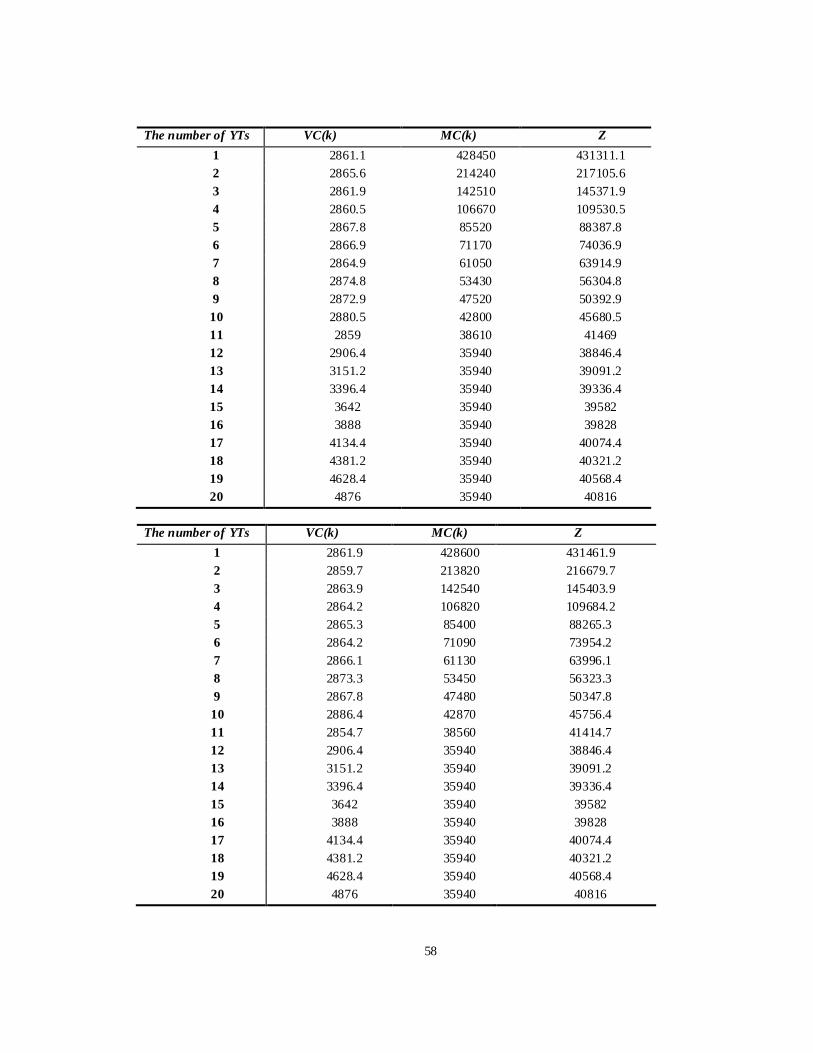
58
The number of YTs VC(k) MC(k) Z
1 2861.1 428450 431311.1
2 2865.6 214240 217105.6
3 2861.9 142510 145371.9
4 2860.5 106670 109530.5
5 2867.8 85520 88387.8
6 2866.9 71170 74036.9
7 2864.9 61050 63914.9
8 2874.8 53430 56304.8
9 2872.9 47520 50392.9
10 2880.5 42800 45680.5
11 2859 38610 41469
12 2906.4 35940 38846.4
13 3151.2 35940 39091.2
14 3396.4 35940 39336.4
15 3642 35940 39582
16 3888 35940 39828
17 4134.4 35940 40074.4
18 4381.2 35940 40321.2
19 4628.4 35940 40568.4
20 4876 35940 40816
The number of YTs VC(k) MC(k) Z
1 2861.9 428600 431461.9
2 2859.7 213820 216679.7
3 2863.9 142540 145403.9
4 2864.2 106820 109684.2
5 2865.3 85400 88265.3
6 2864.2 71090 73954.2
7 2866.1 61130 63996.1
8 2873.3 53450 56323.3
9 2867.8 47480 50347.8
10 2886.4 42870 45756.4
11 2854.7 38560 41414.7
12 2906.4 35940 38846.4
13 3151.2 35940 39091.2
14 3396.4 35940 39336.4
15 3642 35940 39582
16 3888 35940 39828
17 4134.4 35940 40074.4
18 4381.2 35940 40321.2
19 4628.4 35940 40568.4
20 4876 35940 40816

59
The number of YTs VC(k) MC(k) Z
1 2858.3 428050 430908.3
2 2858.3 213700 216558.3
3 2869.4 142840 145709.4
4 2858.8 106630 109488.8
5 2865 85370 88235
6 2870.2 71260 74130.2
7 2869.8 61170 64039.8
8 2869.8 53360 56229.8
9 2877.3 47600 50477.3
10 2877.6 42760 45637.6
11 2857.8 38610 41467.8
12 2906.4 35940 38846.4
13 3151.2 35940 39091.2
14 3396.4 35940 39336.4
15 3642 35940 39582
16 3888 35940 39828
17 4134.4 35940 40074.4
18 4381.2 35940 40321.2
19 4628.4 35940 40568.4
20 4876 35940 40816
The number of YTs VC(k) MC(k) Z
1 2859.6 428220 431079.6
2 2861.2 213950 216811.2
3 2865.4 142610 145475.4
4 2861.6 106570 109431.6
5 2863.2 85330 88193.2
6 2866.4 71160 74026.4
7 2867.7 61150 64017.7
8 2876.8 53490 56366.8
9 2873.9 47580 50453.9
10 2888.6 42920 45808.6
11 2860.1 38630 41490.1
12 2906.4 35940 38846.4
13 3151.2 35940 39091.2
14 3396.4 35940 39336.4
15 3642 35940 39582
16 3888 35940 39828
17 4134.4 35940 40074.4
18 4381.2 35940 40321.2
19 4628.4 35940 40568.4
20 4876 35940 40816
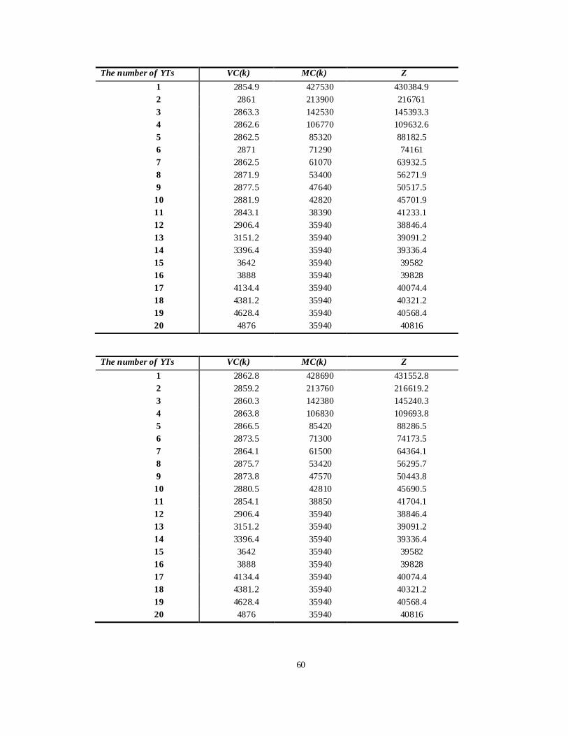
60
The number of YTs VC(k) MC(k) Z
1 2854.9 427530 430384.9
2 2861 213900 216761
3 2863.3 142530 145393.3
4 2862.6 106770 109632.6
5 2862.5 85320 88182.5
6 2871 71290 74161
7 2862.5 61070 63932.5
8 2871.9 53400 56271.9
9 2877.5 47640 50517.5
10 2881.9 42820 45701.9
11 2843.1 38390 41233.1
12 2906.4 35940 38846.4
13 3151.2 35940 39091.2
14 3396.4 35940 39336.4
15 3642 35940 39582
16 3888 35940 39828
17 4134.4 35940 40074.4
18 4381.2 35940 40321.2
19 4628.4 35940 40568.4
20 4876 35940 40816
The number of YTs VC(k) MC(k) Z
1 2862.8 428690 431552.8
2 2859.2 213760 216619.2
3 2860.3 142380 145240.3
4 2863.8 106830 109693.8
5 2866.5 85420 88286.5
6 2873.5 71300 74173.5
7 2864.1 61500 64364.1
8 2875.7 53420 56295.7
9 2873.8 47570 50443.8
10 2880.5 42810 45690.5
11 2854.1 38850 41704.1
12 2906.4 35940 38846.4
13 3151.2 35940 39091.2
14 3396.4 35940 39336.4
15 3642 35940 39582
16 3888 35940 39828
17 4134.4 35940 40074.4
18 4381.2 35940 40321.2
19 4628.4 35940 40568.4
20 4876 35940 40816
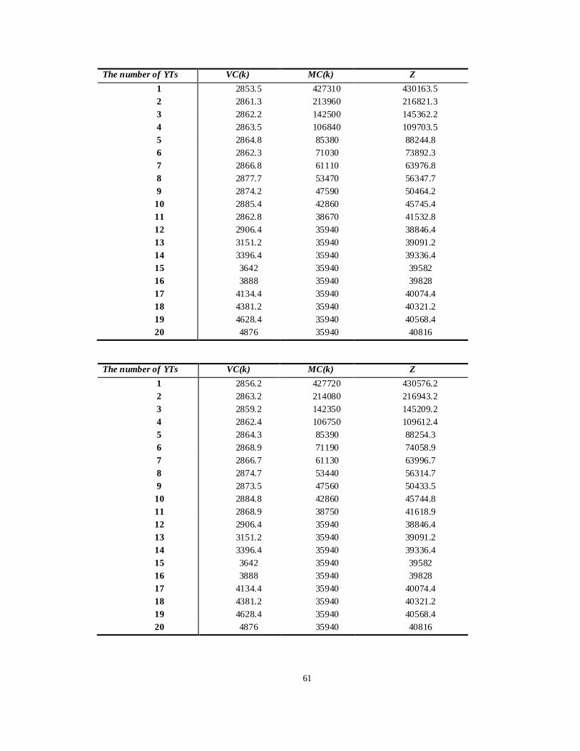
61
The number of YTs VC(k) MC(k) Z
1 2853.5 427310 430163.5
2 2861.3 213960 216821.3
3 2862.2 142500 145362.2
4 2863.5 106840 109703.5
5 2864.8 85380 88244.8
6 2862.3 71030 73892.3
7 2866.8 61110 63976.8
8 2877.7 53470 56347.7
9 2874.2 47590 50464.2
10 2885.4 42860 45745.4
11 2862.8 38670 41532.8
12 2906.4 35940 38846.4
13 3151.2 35940 39091.2
14 3396.4 35940 39336.4
15 3642 35940 39582
16 3888 35940 39828
17 4134.4 35940 40074.4
18 4381.2 35940 40321.2
19 4628.4 35940 40568.4
20 4876 35940 40816
The number of YTs VC(k) MC(k) Z
1 2856.2 427720 430576.2
2 2863.2 214080 216943.2
3 2859.2 142350 145209.2
4 2862.4 106750 109612.4
5 2864.3 85390 88254.3
6 2868.9 71190 74058.9
7 2866.7 61130 63996.7
8 2874.7 53440 56314.7
9 2873.5 47560 50433.5
10 2884.8 42860 45744.8
11 2868.9 38750 41618.9
12 2906.4 35940 38846.4
13 3151.2 35940 39091.2
14 3396.4 35940 39336.4
15 3642 35940 39582
16 3888 35940 39828
17 4134.4 35940 40074.4
18 4381.2 35940 40321.2
19 4628.4 35940 40568.4
20 4876 35940 40816
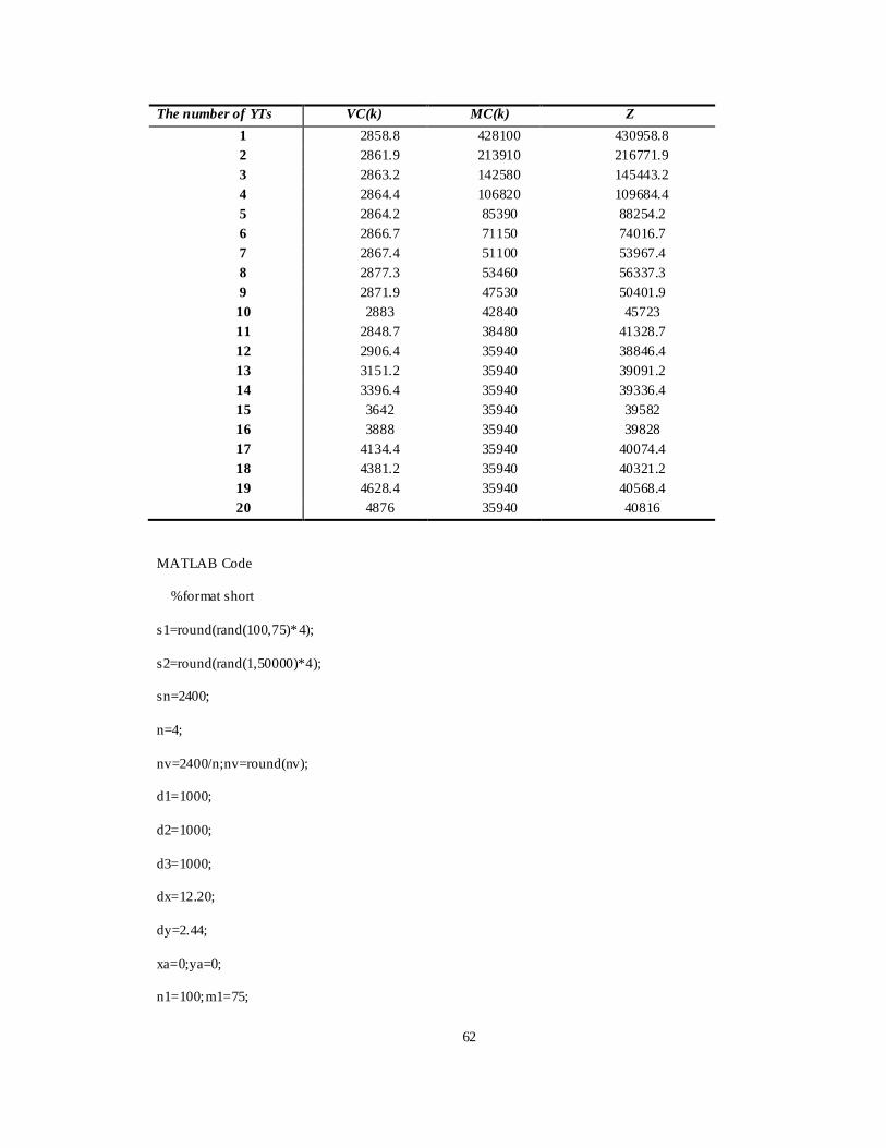
62
The number of YTs VC(k) MC(k) Z
1 2858.8 428100 430958.8
2 2861.9 213910 216771.9
3 2863.2 142580 145443.2
4 2864.4 106820 109684.4
5 2864.2 85390 88254.2
6 2866.7 71150 74016.7
7 2867.4 51100 53967.4
8 2877.3 53460 56337.3
9 2871.9 47530 50401.9
10 2883 42840 45723
11 2848.7 38480 41328.7
12 2906.4 35940 38846.4
13 3151.2 35940 39091.2
14 3396.4 35940 39336.4
15 3642 35940 39582
16 3888 35940 39828
17 4134.4 35940 40074.4
18 4381.2 35940 40321.2
19 4628.4 35940 40568.4
20 4876 35940 40816
MATLAB Code
%format short
s1=round(rand(100,75)*4);
s2=round(rand(1,50000)*4);
sn=2400;
n=4;
nv=2400/n;nv=round(nv);
d1=1000;
d2=1000;
d3=1000;
dx=12.20;
dy=2.44;
xa=0;ya=0;
n1=100;m1=75;
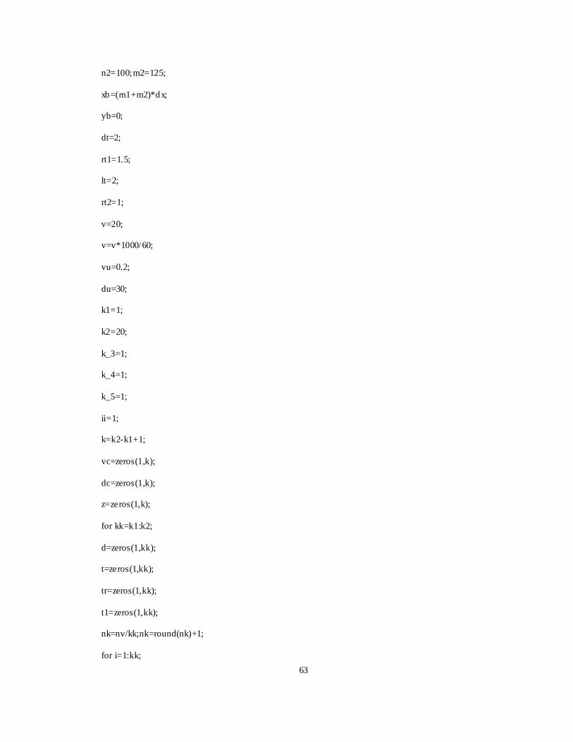
63
n2=100;m2=125;
xb=(m1+m2)*dx;
yb=0;
dt=2;
rt1=1.5;
lt=2;
rt2=1;
v=20;
v=v*1000/60;
vu=0.2;
du=30;
k1=1;
k2=20;
k_3=1;
k_4=1;
k_5=1;
ii=1;
k=k2-k1+1;
vc=zeros(1,k);
dc=zeros(1,k);
z=zeros(1,k);
for kk=k1:k2;
d=zeros(1,kk);
t=zeros(1,kk);
tr=zeros(1,kk);
t1=zeros(1,kk);
nk=nv/kk;nk=round(nk)+1;
for i=1:kk;
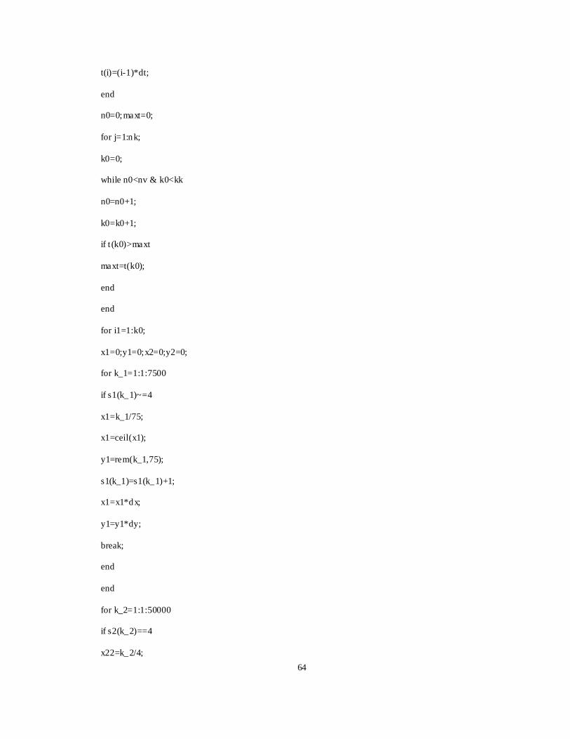
64
t(i)=(i-1)*dt;
end
n0=0;maxt=0;
for j=1:nk;
k0=0;
while n0<nv & k0<kk
n0=n0+1;
k0=k0+1;
if t (k0)>maxt
maxt=t(k0);
end
end
for i1=1:k0;
x1=0;y1=0;x2=0;y2=0;
for k_1=1:1:7500
if s1(k_1)~=4
x1=k_1/75;
x1=ceil(x1);
y1=rem(k_1,75);
s1(k_1)=s1(k_1)+1;
x1=x1*dx;
y1=y1*dy;
break;
end
end
for k_2=1:1:50000
if s2(k_2)==4
x22=k_2/4;
65
x22=ceil(x22);
x2=x22/125;
x2=ceil(x2);
y2=rem(x22,125);
s2(k_2)=0;
x2=x2*dx;
y2=y2*dy;
break;
end
end
if k_2==50000
for k_3=1:1:50000
if s2(k_3)==3
x22=k_2/4;
x22=ceil(x22);
x2=x22/125;
x2=ceil(x2);
y2=rem(x22,125);
s2(k_3)=0;
x2=x2*dx;
y2=y2*dy;
break;
end
end
end
if k_3==50000
for k_4=1:1:50000
if s2(k_4)==2
66
x22=k_2/4;
x22=ceil(x22);
x2=x22/125;
x2=ceil(x2);
y2=rem(x22,125);
s2(k_4)=0;
x2=x2*dx;
y2=y2*dy;
break;
end
end;
end;
if k_4==50000
for k_5=1:1:50000
if s2(k_3)==1
x22=k_2/4;
x22=ceil(x22);
x2=x22/125;
x2=ceil(x2);
y2=rem(x22,125);
s2(k_5)=0;
x2=x2*dx;
y2=y2*dy;
break;
end
end
end
d(i1)=d1+d2+d3+abs(xa-x1)+abs(ya-y1)+abs(x1-(x2+m1))+abs(y1-y2)+abs(x2+m1-xb)+abs(y2-yb);

67
t1(i1)=t(i1)+dt+d(i1)/v+rt1+rt2+lt;
end; % for i1=1:k0
tr=sort(t1);
if t r(1)-t(kk)<=dt
tr(1)=t(kk)+dt;
end;
for j1=1:k0-1;
if t r(j1+1)-tr(j1)<=dt
tr(j1+1)=tr(j1)+dt;
end;
end;
for j1=1:k0;
t(j1)=t r(j1);
end;
end; % for j=1:nk
k3=kk-k1+1;
vc(k3)=0;
for i=1:kk;
vc(k3)=vc(k3)+t(i);
end;
vc(k3)=vc(k3)*vu;
dc(k3)=maxt*du;
z(k3)=vc(k3)+dc(k3);
kkkk(ii)=kk;
ii=ii+1;
vc
dc
68
z
figure
xlabel('kk');
ylabel('vc');
figure
plot(kkkk,dc,'+')
xlabel('kk');
ylabel('dc');
figure
plot(kkkk,z,'+');
xlabel('kk');
ylabel('z')
69
REFERENCES
AXS-Alphaliner. Data on November 11th, 2008
Avriel, M. and Penn, M.. 1993. Exact and Approximate Solutions of the Containership
Stowage Problems,” Computer and Industrial Engineering, 25 :271-274.
Avriel, M., Penn M. and Shriper N.. 2000. Container Ship Stowage Problem:
Complexityand Connection to the Coloring of Circle Graphs [J]. Discrete Applied Mathematics ,
103:271-279.
Avriel, M., Penn M., Shriper N. and Witteboon S. 1998. Stowage Planning for
Containerships to Reduce the Number of Shifts[J]. Annals of Operation Research, 76: 55-71.
Bish, Ebru K.. 2003. A mult iple-crane-constrained scheduling problem in a container
Terminal[J]. European Journal of Operational Research, 144 (1): 83-107.
CBS: “Container transport increasingly important”, Web magazine, 22 January 2009 15:00,
http://www.cbs.nl/enGB/menu/themas/verkeervervoer/publicaties/artikelen/archief/2009/2009 -
2648-wm.htm.
CAO Jinxin, SHI Qixin, Der-Horng Lee. 2008. A Decision Support Method for Truck
Scheduling and Storage Allocation Problem at Containe[J]. TSINGHUA SCIENCE AND
TECHNOLOGY, 13(1) :211-216.
Chuqian Zhang, Yat-wah Wan, Jiy in Liu, Richard J. Linn. 2002. Dynamic crane
deploymentin container storage yard[J]. Transportation Research Part B, 36: 537-555.
Daganzo, Carlos F.. 1989. The crane scheduling problem[J]. Transportation Research Part
B, 23 (3): 159-175.
Der-Horng Lee, Hui Qiu Wang , Lixin Miao.2008. Quay crane scheduling with non-
interference constraints in port container terminals [J]. Transportation Research Part E, 44:124-135.
Dirk Steenken, Stefan Vo and Robert Stahlbock. 2004. Container terminal operation and

70
operations research- a classification and literature review[J]. OR Spectrum, 26:3-49.
Erhan Kozan, Peter Preston. 1999. Genetic algorithms to schedule container transfers at mult imodal
terminals[J]. International Transportations in Operations Research. 6:311-329
Eric Ting. Container Terminal Operat ion and Cargo Handling” Department of
transportation and Navigation Science, National Taiwan Ocean University
http://ind.ntou.edu.tw/~ericting/download/Container%20Transport/06%20Container%20Terminal%
20Operation.pdf
Evangelos Kaisar. 2006. A STOWAGE PLANNING MODEL FOR MULTIPORT
CONTAINER TRANSPORTATION., Doctor of Philoshophy, Dissertation, University of Maryland.
Glover Fred. 1989. Tabu Search, Part I. ORSA Journal on Computing, 1(3): 190-206.
Glover Fred. 1990. Tabu Search-Part Ⅱ . ORSA Journal on Computing 2(1)
Glover Fred. 2001. Tabu Search : A Tutorial
http://www.cse.unt.edu/~garlick/teaching/4310/assign/TS%20-%20Tutorial.pdf
Golberg, D.E, and Lingle, R.. 1985. Loci and Traveling Sales man Problem.
Proceedings of an International Conference on Genetic Algorithms an Their Applicat ions, Lawrence
Eribaum Associates, Hillsdale, NJ.
Goodchild, A.V., Daganzo, C.F.. 2007. Crane double cycling in container ports: planning
methods and evaluation[J]. Transportation Research Part B 41 (8), 875- 891.
Haiq ing Zhang, Jun Li, Shunguo Lan. 2008. Research of Container Truck deployment.
Logistics SEI-TECH.
Henry Y.K. Lau, Ying Zhao. 2008. Integrated scheduling of handling equipment at
automated container terminals. Int. J. Production Economics 112:665-682.
Imai, Akio, Sun, Xin, Nishimura, Etsuko, 2005. Berth allocation in a container port:
using a continuous location space approach[J]. Transportation Research Part B, 39 (3):199-221.
Ioannou, P., Kos matopoulos, E.B., Jula, H., Collinge, A., Liu, C.-I., Asef-vaziri, A., Dougherty Jr., E., 2000.
Cargo handling technologies. Final Report, University of Southern Californ ia.
http://www.usc.edu/dept/ee/catt/2002/ju la/Marine/FinalReport_CCDoTT_97.pdfS
Jens Clausen, 1999. Branch and Bound Algorithms-Principles and Examples.
71
Jonathan Pengelly. MONTE CARLO METHODS”,tutorial, University of Otago
http://www.cs.otago.ac.nz/cosc453/student_tutorials/monte_carlo.pdf
Joy Woller. 1996. The Basics of Monte Carlo Simulations .
http://www.chem.unl.edu/zeng/joy/mclab/mcintro.html
Kaisar, E.. 1999. An optimal Model for Optimal Container Loading . M.S.. Thesis,
University of Mary land.
Kap Hwan Kim a, Ki Young Kim. 2007. Optimal price schedules for storage of in bound
containers[J]. Transportation Research Part B, 41: 892-905.
Kim, K.H., Bae, J.W., 1999. A dispatching method for automated guided vehicles to
minimize delays of containership operations[J]. International Journal of Management Science, 5
(1): 1-25.
Kim, K.H., Bae, J.W.. 2004. A look-ahead dispatching method or automated guided
vehicles in automated port container terminal[J]. Transportation Science 38(2):224-234.
Kim, K.H., Kim, K.Y.. 1999. A routing algorithm for a single straddle carrier to load
export containers onto a containership[J]. International Journal of Production Economics , 59:425-
433.
Kim, K.H., Kim, K.Y., 1999. An optimal routing algorithm for a transfer crane in port
container terminals[J]. Transportation Science, 36:109-136.
Kim, K.H., Kim, K.Y.. 1999. Routing straddle carriers for the loading operation of
containers using a beam search algorithm[J]. Computers and Industrial Engineering, 36: 109-136.
Kim, K.H., Park, Y.M., 2004. A crane scheduling method for port container terminals [J].
European Journal of Operational Research, 156 (3): 752-768.
Kim, Kap Hwan, Lee, Keung Mo, Hwang, Hark, 2003. Sequencing delivery and receiv ing
operations for yard cranes in port container terminals[J]. International Journal of Production
Economics, 84 (3): 283-292.
Lau, Henry Y.K., Zhao Ying. 2008. Integrated scheduling of handling equipment at
automated container terminals[J]. International Journal of Production Economics , 112 (2):665-682.
Lee, D.-H., Cao, Z., Meng, Q. 2007. Scheduling of two transtainer systems for loading
72
outbound containers in port container terminals with simulated annealing algorithm[J]. International
Journal of Production Economics , 107:115-124.
Lim, A., Rodrigues, B., Xiao, F., Zhu, Y., 2004. Crane scheduling with spatial constraints. Naval Research
Logistics 51, 386–406.
Liu, Chin -I., Ioannou, P.A., 2002. A comparison of different AGV dispatching rules in an
automated container terminal. In : The IEEE Fifth Conference on Intelligent Transportation Systems
Singapore. pp. 880-885.
Lu Chen, Nathalie Bostel, Pierre Dejax, Jianguo Cai, Lifeng Xi. 2007. A tabu search
algorithm for the integrated scheduling problem of container handling systems in a maritime
terminal[J]. European Journal of Operational Research 181:40-58.
Matthew E.H. Petering. 2009. Effect of b lock width and storage yard layout on marine
container terminal performance[J]. Transportation Research Part E, 45: 591-610.
Meersmans, P.J.M., 2002. Optimizat ion of container handling
systems. Thela Thesis, Amsterdam
Ng, W.C.. 2005. Crane scheduling in container yards with inter-crane interference[J].
European Journal of Operational Research, 164 (1): 64-78.
Nishimura, Etsuko, Imai, Akio, Stratos, Papadimitriou. 2001. Berth allocation planning in
the public berth system by genetic algorithms[J]. European Journal of Operational Research, 131
(2):282-292.
Nishimura, Etsuko, Imai, Akio, Stratos, Papadimitriou. 2005. Yard trailer routing at a
maritime container terminal[J]. Transportation Research Part E, 41 (1): 53-76.
Patrick J.M.Meers mans, Albert P.M. Wagelmans. 2001. Effective algorithms for
intergraged scheduling of handling equipment at automated containers terminal. ERIM REPORT
SERIES RESEARCH IN MANAGEMENT, 3-31.
Patrick J.M.Meers mans, Romment Dekker. 2001. Opearation Research Support
Container Handling. Ecnometric Institute Report, 1-22.
Peterk, Roy I., Daganzo, Carlos F..1990. A branch and bound solution method for
the crane scheduling problem[J]. Transportation Research Part B, 24 (3):159-172.
73
PHOTI S M PANAYIDES. 2006. Marit ime Logistics and Global Supply Chains:
Towards a Research Agenda[J]. Maritime Economics & Logistics. 8:3-18.
P. Jaime Tetrault.2004. The Container Revolution: 50 years of Industry Change
https://caterpillar.lithium.com/t5/BLOG-MARINE-INSIGHT/The-Container-Revolution-50-years-
of-Industry-Change/ba-p/2004
Qingcheng Zeng, ZhongzhenYang , Luyuan Lai.2009. Models and algorithms for mult i-
crane oriented scheduling method in container terminals [J]. Transport Policy, 16:271-278.
Ralph udo gasser. 1995. Harnessing Computational Resources for Efficient Exhaustive
Search. Diss. ETH ,10:9-27
R.K. Cheung, C.L. Li, W. Lin. 2002. Interblock crane deployment in container
terminals[J], Transport. Sci. ,36:79-93.
Robert Stahlbock and Stefan Voß. Operations research at container terminals: a literature
update. 2008. Operations research at container terminals: a literature update. OR Spectrum. 30:1-
52.
The Design & Analysis of Algorithms, 2nd
edition. 2007.
http://www.slidefinder.net/C/ch03n/29173413.
THEO NOTTEBOOM, JEAN-PAUL RODRI GUE. 2008. Containerisation, Box
Logistics and Global Supply Chains: The Integration of Ports and Liner Shipping Networks [J].
Maritime Economics & Logistics. 10:152-174.
W.C. Ng, K.L. Mak. Yard crane scheduling in port container terminals [J]. 2005. Applied
Mathematical Modelling. 29 : 263-276.
W. Winklemans, et.al.. 2002. Prt competit iveness: an economic and legal analysis of the
factors determining the competit iveness of seaports.
Xi Guo, Shell Ying Huang, Wen Jing Hsu and Malcolm Yoke Hean Low. 2009.
Simulation-Based Dynamic Partit ioning of Yard Crane Workload for Container Terminal
Operations. Proceeding SpringSim '09 Proceedings of the 2009 Spring Simulat ion Multiconference .
society for Computer Simulation International San Diego, CA, USA publisher.
Zyngiridis, I. 2005. Optimizing container movements using one and two automated

74
stacking cranes. Master‟s thesis, Naval Postgraduate School, Monterey.