Modeling and Querying Spatial DataWarehouses on the Semantic Web

Nurefsan Gur1(B), Katja Hose1, Torben Bach Pedersen1,and Esteban Zimanyi2

1 Aalborg University, Aalborg, Denmark{nurefsan,khose,tbp}@cs.aau.dk

2 Universite Libre de Bruxelles, Brussels, Belgiumezimanyi@ulb.ac.be

Abstract. The Semantic Web (SW) has drawn the attention of dataenthusiasts, and also inspired the exploitation and design of multidimen-sional data warehouses, in an unconventional way. Traditional data ware-houses (DW) operate over static data. However multidimensional (MD)data modeling approach can be dynamically extended by defining boththe schema and instances of MD data as RDF graphs. The importanceand applicability of MD data warehouses over RDF is widely studiedyet none of the works support a spatially enhanced MD model on theSW. Spatial support in DWs is a desirable feature for enhanced analy-sis, since adding encoded spatial information of the data allows to querywith spatial functions. In this paper we propose to empower the spatialdimension of data warehouses by adding spatial data types and topolog-ical relationships to the existing QB4OLAP vocabulary, which alreadysupports the representation of the constructs of the MD models in RDF.With QB4SOLAP, spatial constructs of the MD models can be also pub-lished in RDF, which allows to implement spatial and metric analysison spatial members along with OLAP operations. In our contribution,we describe a set of spatial OLAP (SOLAP) operations, demonstrate aspatially extended metamodel as, QB4SOLAP, and apply it on a use casescenario. Finally, we show how these SOLAP queries can be expressedin SPARQL.

1 Introduction

The evolution of the Semantic Web (SW) and its tools allow to employ com-plex analysis over multidimensional (MD) data models via On-Line Analyti-cal Processing (OLAP) style queries. OLAP emerges when executing complexqueries over data warehouses (DW) to support decision making. DWs store largevolumes of data which are designed with MD modeling approach and usuallyperceived as data cubes. Cells of the cube represent the observation facts foranalysis with a set of attributes called measures (e.g. a sales fact cube withmeasures of product quantity and prices). Facts are linked to dimensions whichgive contextual information (e.g. sales date, product, and location). Dimensionsare perspectives which are used to analyze data, organized into hierarchies andc© Springer International Publishing Switzerland 2016G. Qi et al. (Eds.): JIST 2015, LNCS 9544, pp. 3–22, 2016.DOI: 10.1007/978-3-319-31676-5 1

4 N. Gur et al.

levels that allow users to analyze and aggregate measures at different levels ofdetail. Levels have a set of attributes that describe the characteristics of the levelmembers.

In traditional DWs, the “location” dimension is widely used as a conventionaldimension which is represented in an alphanumeric manner with only nominalreference to the place names. This neither allow manipulating location-baseddata nor deriving topological relations among the hierarchy levels of the locationdimension. This issue yields a demand for truly spatial DWs for better analysispurposes. Including encoded geometric information of the location data signif-icantly improves the analysis process (i.e. proximity analysis of the locations)with comprehensive perspectives by revealing dynamic spatial hierarchy levelsand new spatial members. The scope of this work is first focuses on enhancingthe spatial characteristics of the cube members on the SW, and then describingand utilizing SOLAP operators for advanced analysis and decision making.

In our approach we consider enabling SOLAP capabilities directly overResource Description Framework (RDF) data on the SW. Importance andapplicability of performing OLAP operations directly over RDF data is studiedin [9,12]. To perform SOLAP over the SW consistently, an explicit and precisevocabulary is needed for the modeling process. The key concepts of spatial cubemembers need to be defined in advance to realize SOLAP operations since theyemploy spatial measures with spatial aggregate functions (e.g. union, buffer,and, convex-hull) and topological relations among spatial dimension and hierar-chy level members (e.g. within, intersects, and, overlaps). Current state of theart RDF and OLAP technologies is limited to support conventional dimensionschema and analysis along it’s levels. Spatial dimension schema and SOLAPrequire an advanced specialized data model. As a first effort to overcome thelimitations of modeling and querying spatial data warehouses on the SemanticWeb we give our contributions in the following.

Contributions. We propose an extended metamodel solution that enables rep-resentation and RDF implementation of spatial DWs. We base our metamodel onthe most recent QB4OLAP vocabulary and present an extension to support thespatial functions and spatial elements of the MD cubes. We discuss the notionof a SOLAP operator and observe it with examples, then we give the semanticsof each SOLAP operator formally and finally, show how to implement them inSPARQL by using sub-queries and nested set of operators.

In the remainder of the paper, we first present the state of the art, in Sect. 2.As a prerequisite for our contribution in Sect. 3, we give the preliminary conceptsand explain the structure of a SOLAP operator. Then, in Sect. 4 we define thesemantics of MD data cube elements in RDF, present QB4SOLAP and formalizethe SOLAP operators over MD data cube elements. We present a QB4SOLAPuse case in Sect. 5 and then, we show how to write the defined SOLAP queriesover this use case in SPARQL in Sect. 6. Finally, in Sect. 7, we conclude andremark to the future work directions.

Modeling and Querying Spatial Data Warehouses on the Semantic Web 5

2 State of the Art

DW and OLAP technologies have been proven a successful approach for analysispurposes on large volumes of data [1]. Aligning DW/OLAP technologies withRDF data makes external data sources available and brings up dynamic sce-narios for analysis. The following studies are found concerning DW/OLAP withthe SW.

DW/OLAP and Semantic Web: The potential of OLAP to analyze SWdata is recognized in several approaches, thus MD modeling from ontologies isstudied in the works of [8,17]. However these approaches do not support standardquerying of RDF data in SPARQL but require a MD or a relational databasequery engine, which limits the access to frequently updated RDF data. Kampgenet al. propose an extended model [12] on top of RDF Data Cube Vocabulary(QB) [6] for interacting with statistical linked data via OLAP operations inSPARQL, but it has the limitations of the QB and thus cannot support fullOLAP dimension structure with aggregate functions. It also has only limitedsupport for complete MD data model members (e.g. hierarchies and levels).Etcheverry et al. introduce QB4OLAP [9] as an extended vocabulary of QBwith a full MD metamodel, which supports OLAP operations directly over RDFdata with SPARQL queries. However, none of these vocabularies and approachessupport spatial DWs, unlike our proposal.

Spatial DW and OLAP: The constraint representation of spatial data hasbeen focus in many fields from databases to AI [18]. Extending OLAP withspatial features has attracted the attention of data warehousing communities aswell. Several conceptual models are proposed for representing spatial data in datawarehouses. Stefanovic et al. [11] investigates on constructing and materializingthe spatial cubes in their proposed model. The MultiDim conceptual model isintroduced by Malinowski and Zimanyi [16] which copes with spatial featuresand extended in [20], to include complex geometric features (i.e. continuousfields), with a set of operations and MD calculus supporting spatial data types.Gomez et al. [10] propose an algebra and a very general framework for OLAPcube analysis on discrete and continuous spatial data. Even though spatial datawarehousing is widely studied, it has not implemented yet on the Semantic Web.

Geospatial Semantic Web: The Open Geospatial Consortium – OGC pursuean important line of work for geospatial SW with GeoSPARQL [3] as a vocabu-lary to represent and query spatial data in RDF with an extension to SPARQL.Kyzirakos et al. presents a comprehensive survey in data models and query lan-guages for linked geospatial data in [14], and propose a semantic geospatial datastore - Strabon with an extensive query language – stSPARQL in [13], whichis yet limited to a specific environment. LinkedGeoData is a significant contri-bution on interactively transforming OpenStreetMap1 data to RDF data [19].GeoKnow [15] is a more recent project with focus on linking geospatial datafrom heterogeneous sources.1 http://www.openstreetmap.org.

6 N. Gur et al.

The studies shows that, SW and RDF technologies evolve to give better func-tionality and standards for spatial data representation and querying. It is alsoargued above that spatial data is very much needed for DW/OLAP applications.However modeling and querying of spatial DWs on the SW is not addressed inany of the above papers. There are recent efforts on creating an Extract-Load-Transform (ETL) framework from semantic data warehouses [7] and publishing/-converting open spatial data as Linked Open Data [2], which motivates modelingand querying spatial data warehouses on the Semantic Web. Spatial data requiresspecific treatment techniques, particular encoding, special functions and differ-ent manipulation methods, which should be considered during the design andmodeling process. Current state of the art geospatial Semantic Web focuses ontechniques for publishing, linking and querying spatial data however does notelaborate on analytical spatial queries for MD data. In order to address theseissues we propose a generic and extensible metamodel based on the best practicesof MD data publishing in RDF. Then we show how to create spatial analyticalqueries with SOLAP on MD data models. We base ourselves on existing worksby extending the most recent version of the QB4OLAP vocabulary with spatialconcepts. Furthermore, we introduce the new concept of SOLAP operators thatnavigate along spatial dynamic hierarchy levels and implement these analyticalspatial queries in SPARQL.

3 Spatial and OLAP Operations

In this section we give define the spatial and spatial OLAP (SOLAP) operations.

3.1 Spatial Operations

In order to understand spatial operations, it is important to understand what isa spatial object. A spatial object is the data or information that identifies a real-world entity of geographic features, boundaries, places etc. Spatial objects canbe represented in object/vector or image/raster mode. Database applicationsthat can store spatial objects need to specify the spatial characteristics, encodedas specific information such as geometry data type which is the most commonand supports planar or Euclidean (flat-earth) data. Point, Line, and, Polygonare the basic instantiable types of the geometry data type.

Geometries are associated with a spatial reference system (SRS) whichdescribes the coordinate space in which the geometry is defined. There are severalSRSs and each of them are identified with a spatial reference system identifier(SRID). The World Geodetic System (WGS) is the most well-known SRS andthe latest version is called WGS84, which is also used in our use case.

Spatial data types have a set of operators that can function among applica-tions. We grouped these operations into classes. Our classification is based onthe common functionality of the operators. These classes are defined as follows:

Spatial Aggregation. The operators in the spatial aggregation, Sagg classaggregate two or more spatial objects. The result of these operators returns

Modeling and Querying Spatial Data Warehouses on the Semantic Web 7

a new composite spatial object. Union, Intersection, Buffer, ConvexHull, and,MBR - Minimum Bounding Rectangle are example operators of this class.

Topological Relation. The operators in the topological relation, Trel class arecommonly contained in the RCC82 and DE-9DIM3 models. Topological relationsare standardized by OGC as Boolean operators which specify how two spatialobjects are related to each other with a set of spatial predicates for example:Intersects, Disjoint, Equals, Overlaps, Contains, Within, Touches, Covers, Cov-eredBy, and, Crosses.

Numeric Operation. The operators in the class of numeric operation, Nop

take one or more spatial objects and return a numeric value. Perimeter, Area,# of Interior Rings, Distance, Haversine Distance, Nearest Neighbor (NN), and# of Geometries are some of the example operators of this class.

3.2 SOLAP Operations

OLAP operations emerge when executing complex queries over multidimensional(MD) data models. OLAP operations let us interpret data from different per-spectives at different levels of detail. Spatially extended multidimensional modelsincorporate spatial data during the analysis and decision making process byrevealing new patterns, which are difficult to discover otherwise. In connectionwith our definition of MD models in the first paragraph of Sect. 1, hereafter weenhance and describe the spatially extended MD data cube elements.

A spatially extended MD model contains both conventional and spatialdimensions. A spatial dimension is a dimension which includes at least one spatialhierarchy. Dimensions usually have more than one level which are representedthrough hierarchies and there is always a unique top level All with just onemember. A hierarchy is a spatial hierarchy if it has at least one spatial level inwhich the application should store the spatial characteristics of the data, whichis captured by it is geometry and can be recorded in the spatial attributes ofthe level. A spatial fact is a fact that relates several dimensions in which, twoor more are spatial. For example, consider a “Sales” spatial fact cube, whichhas “Customer” and “Supplier” (company) as spatial dimensions with a spatialhierarchy as “Geography” that expands into (hierarchic) spatial levels; “City →State → Country → Continent → All” from the customer and supplier’s loca-tion. All these spatial levels record the spatial characteristics i.e. with a spatialattribute of a city (center) as “point” coordinates. Measures in the cube expressadditional and essential information for each MD data cell which is not exhibitedthrough the dimensions and level attributes. Typically, spatially extended MDmodels have spatial measures which are represented by a geometry i.e. point,polygon, etc.

2 RCC8 – Region Connection Calculus describes regions in Euclidean space, or in atopological space by their possible relations to each other.

3 DE-9DIM – Dimensionally Extended Nine-Intersection Model is a topological modelthat describes spatial relations of two geometries in two-dimensions.

8 N. Gur et al.

Spatial OLAP operates on spatially extended MD models. SOLAPenhances the analytical capabilities of OLAP with the spatial information ofthe cube members. The term SOLAP used in [4] and their similar works asa visual platform, which is designed to analyze huge volumes of geo-referenceddata by providing visualization of pivot tables, graphical displays and interactivemaps. We define the term SOLAP concisely as a platform (and query language)independent high-level concept, which is applicable on any spatial multidimen-sional data. We explain and exemplify in the following how SOLAP operatorsare interpreted.

Each operator in SOLAP should include at least one spatial condition byusing the aforementioned operators from the spatial operation classes definedin Sect. 3.1. Spatial operations in SOLAP create a dynamic interpretation ofthe cube members as a dynamic spatial hierarchy or level. These interpretationsallow new perspectives to analyze the spatial MD data which cannot be accessedin a traditional MD model. For instance, the classical OLAP operator roll-upaggregates measures along a hierarchy to obtain data at a coarser granularity.In the spatial dimension schema Fig. 1, the (classical) roll-up relation, Customerto City is shown with black straight arrows. On the other hand, in SOLAP, anew “dynamic spatial hierarchy” is created on the fly to roll-up among spatiallevels by a spatial condition (closest distance), which is given as Customer toClosest-City (of the Supplier), shown with curved arrows in gray. The details ofthis operator in comparison with OLAP and SOLAP are given in the followingexample.

Example: Roll-up. The user wants to sum the total amount of the salesto customers up to the city level with the roll-up operator. The instancedata for Sales fact is given in Table 1 and shown on the map in Fig. 2.

Fig. 1. S-Dim. Schema Fig. 2. Example map of sales (instance) data

Modeling and Querying Spatial Data Warehouses on the Semantic Web 9

Table 1. Sample (instance) data for sales

City Customer Supplier sales Total saless1 s2 s3

Dusseldorf c1 8pcs. – 3pcs. 11pcs.c2 10pcs. – – 10pcs.

Dortmund c3 7pcs. 4pcs. – 11pcs.c4 – 20pcs. 3pcs. 23pcs.

Munster c5 – – 30pcs. 30pcs.

Table 2. Roll-up

City Sales

Dusseldorf 21pcs.

Dortmund 34pcs.

Munster 30pcs.

Table 3. S-Roll-up

City Sales

Dusseldorf 25pcs.

Dortmund 20pcs.

Munster 33pcs.

Table 4. Customer to Supplier Distance (km.s)

Sup. City Dusseldorf Dortmund Munster

Cust. City Cust.Sup.

s1 s2 s3

Dusseldorf c1 15 km.s 45km.s 30 km.sc2 15 km.s 60 km.s 60 km.s

Dortmund c3 15 km.s 30 km.s 45 km.sc4 45 km.s 15 km.s 15 km.s

Munster c5 60 km.s 45 km.s 15 km.s

The amount of the sales are shown in parentheses along with the quanti-ties of the sold parcels (from supplier to customer). The arrows on the map,between the supplier and customer locations are used to represent the distance.The summarized data for sale instances (Table 1) does not originally containthe records of the supplier – customer distance (as given in Table 4) whichcan lead to increase in the storage space. If there are no sales to customersfrom the corresponding suppliers, a dash (–) is used in Table 1. The syntaxof the traditional roll-up operator is ROLLUP(Sales, (Customer → City),SUM(SalesAmount)) which aggregates the “total sales to customers up tocity level” (results in Table 2). Alternatively, the user may like to view the “totalsales to customers by city of the closest suppliers”, in which some customerscan be closer to their suppliers from other cities, as emphasized in Table 4.This query is possible with traditional OLAP, if only Table 4 is recorded inthe base data which requires extra storage space. For a better support and flex-ibility we define a spatial roll-up operator that aggregates the total sales alongthe dynamic spatial hierarchy, which is created based on a spatial condition(in this example, distance between customer and supplier locations). The syn-tax for s-roll-up is; S-ROLLUP(Sales,[CLOSEST(Customer,Supplier)]→ City’,SUM(SalesAmount)). The spatial condition transforms thecustomer→city hierarchy as a dynamic spatial hierarchy, which depends onthe proximity of the suppliers that is calculated during runtime. The user has theflexibility to make analyses with different spatial operations in SOLAP. Spatialextensions of common OLAP operators (roll-up, drill-down, slice, and dice) areformally defined in Sect. 4.3.

10 N. Gur et al.

4 Semantics of Spatial MD Data and OLAP Operations

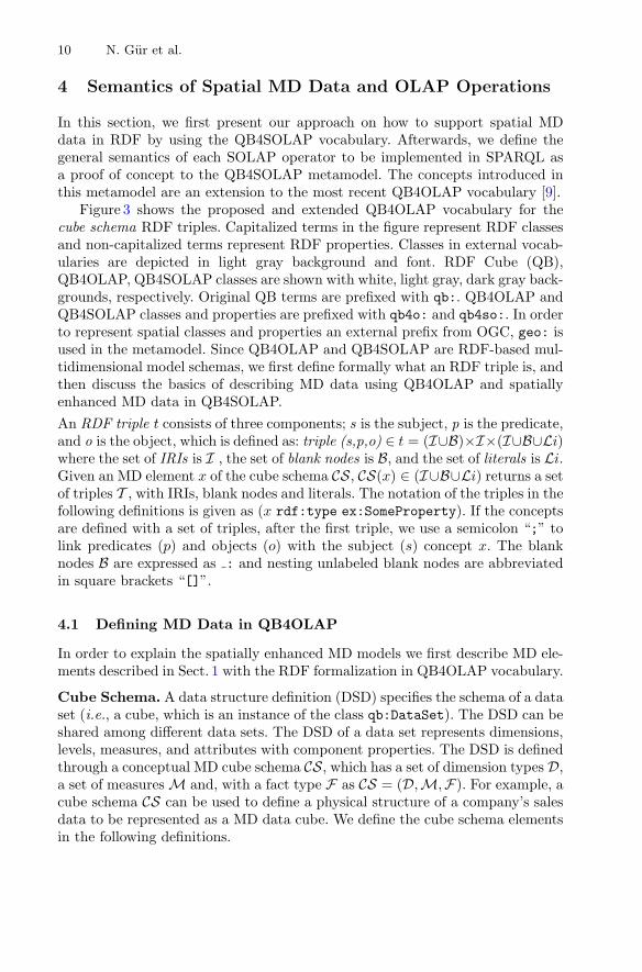
In this section, we first present our approach on how to support spatial MDdata in RDF by using the QB4SOLAP vocabulary. Afterwards, we define thegeneral semantics of each SOLAP operator to be implemented in SPARQL asa proof of concept to the QB4SOLAP metamodel. The concepts introduced inthis metamodel are an extension to the most recent QB4OLAP vocabulary [9].

Figure 3 shows the proposed and extended QB4OLAP vocabulary for thecube schema RDF triples. Capitalized terms in the figure represent RDF classesand non-capitalized terms represent RDF properties. Classes in external vocab-ularies are depicted in light gray background and font. RDF Cube (QB),QB4OLAP, QB4SOLAP classes are shown with white, light gray, dark gray back-grounds, respectively. Original QB terms are prefixed with qb:. QB4OLAP andQB4SOLAP classes and properties are prefixed with qb4o: and qb4so:. In orderto represent spatial classes and properties an external prefix from OGC, geo: isused in the metamodel. Since QB4OLAP and QB4SOLAP are RDF-based mul-tidimensional model schemas, we first define formally what an RDF triple is, andthen discuss the basics of describing MD data using QB4OLAP and spatiallyenhanced MD data in QB4SOLAP.An RDF triple t consists of three components; s is the subject, p is the predicate,and o is the object, which is defined as: triple (s,p,o) ∈ t = (I∪B)×I×(I∪B∪Li)where the set of IRIs is I , the set of blank nodes is B, and the set of literals is Li.Given an MD element x of the cube schema CS, CS(x) ∈ (I∪B∪Li) returns a setof triples T , with IRIs, blank nodes and literals. The notation of the triples in thefollowing definitions is given as (x rdf:type ex:SomeProperty). If the conceptsare defined with a set of triples, after the first triple, we use a semicolon “;” tolink predicates (p) and objects (o) with the subject (s) concept x. The blanknodes B are expressed as : and nesting unlabeled blank nodes are abbreviatedin square brackets “[]”.

4.1 Defining MD Data in QB4OLAP

In order to explain the spatially enhanced MD models we first describe MD ele-ments described in Sect. 1 with the RDF formalization in QB4OLAP vocabulary.

Cube Schema. A data structure definition (DSD) specifies the schema of a dataset (i.e., a cube, which is an instance of the class qb:DataSet). The DSD can beshared among different data sets. The DSD of a data set represents dimensions,levels, measures, and attributes with component properties. The DSD is definedthrough a conceptual MD cube schema CS, which has a set of dimension types D,a set of measures M and, with a fact type F as CS = (D,M,F). For example, acube schema CS can be used to define a physical structure of a company’s salesdata to be represented as a MD data cube. We define the cube schema elementsin the following definitions.

Modeling and Querying Spatial Data Warehouses on the Semantic Web 11

Fig. 3. QB4SOLAP vocabulary meta-model

Attributes. An attribute a ∈ A = {a1, a2, . . . , an} has a domain 〈a : dom〉in the cube schema CS with a set of triples ta ∈ T where ta is encoded as(a rdf:type qb:AttributeProperty; rdfs:domain xsd:Schema)

The domain of the attribute is given with the property rdfs:domain4 fromthe corresponding schema and rdfs:range defines what values the property cantake i.e.; integer, decimal, etc. from the given, xsd:Schema elements5. Attributesare the finest granular elements of the cube, which exists in levels to describethe characteristics of level members e.g., customer level attributes could be as;name, id, address, etc.

Levels. A level l ∈ L = {l1, l2, . . . , ln} consists of a set of attributes Al,which is defined by a schema l(a1 : dom1, . . . , an : domn), where l is the leveland each attribute a is defined over the domain dom. For each level l ∈ L

4 RDF Schema http://www.w3.org/TR/rdf-schema/.5 XML Schema http://www.w3.org/TR/xmlschema11-1/.

12 N. Gur et al.

in the cube schema CS, there is a set of triples tl ∈ T which is encoded as(l rdf:type qb4o:LevelProperty; qb4o:hasAttribute a). Relevant levels forcustomer data include; customer level, city level, country level, etc.

Hierarchies. A hierarchy h ∈ H = {h1, h2, . . . , hn} in the cube schemaCS, is defined with a set of triples th ∈ T , and encoded as (h rdf:typeqb4o:HierarchyProperty; qb4o:hasLevel l; qb4o:inDimension D).

Each hierarchy h ∈ H is defined as h = (Lh,Rh); with a set of Lh (hierarchy)levels, which is a subset of the set Ld levels of the dimension D where Lh ⊆Ld ∈ D. Ld contains the initial base level of the dimension in addition tohierarchy levels Lh. For example, customer–location hierarchy can be definedby the levels; customer, city, country, etc. where customer is the base level andcontained only in Ld.

Due to the nature of the hierarchies, a hierarchy entails a roll-up relation Rh

between its levels, Rh = (Lc,Lp, card) where Lc and Lp are respectively childand parent levels, where the lower level is called child and higher level is calledparent. Cardinality card ∈ {1 − 1, 1 − n, n − 1, n − n} describes the minimumand maximum number of members in one level that can be related to a memberin another level, e.g., Rh = (city, country,many − to − one) shows that theroll-up relation between the child level city to parent level country is many-to-one, which means that each country can have many cities. In order to representcardinalities between the child and the parent levels, blank nodes are createdas hierarchy steps, : hhs ∈ B. Hierarchy steps relate the levels of the hierarchyfrom a bottom (child) level to an upper (parent) level, which is defined with aset of triples ths ∈ T and encoded as (: hhs rdf:type qb4o:HierarchyStep;qb4o:childLevel lhc; qb4o:parentLevel lhp; qb4o:cardinality card) wherelhc ∈ Lc, lhp ∈ Lp and card ∈ {1 − 1, 1 − n, n − 1, n − n}.

Dimensions. An n-dimensional cube schema has a set of dimensions D ={d1, d2, . . . , dn}. And each d ∈ D is defined as a tuple d = (L,H); with a setof Ld levels, organized into Hd hierarchies. Dimensions, inherently have all thelevels from the hierarchies they have, and an initial base level. For each dimen-sion d ∈ D, in the cube schema CS, there is a set of triples td ∈ T , which isencoded as (d rdf:type qb:DimensionProperty; qb4o:hasHierarchy h). Forexample, customerDim is a dimension with a location and a customer type hier-archy where location expands to levels of customer’s location (e.g., city, country,etc.) and customer type expands to levels of customer’s type (e.g.,profession,branch, etc.).

Measures. A measure m ∈ M = {m1,m2, . . . ,mn}, is a property, whichis associated to the facts. Measures are given in the cube schema CS witha set of triples tm ∈ T , which is encoded as (mrdf:type qb:MeasureProperty;rdfs:subPropertyOf sdmx-measure:obsValue; rdfs:domain xsd:Schema).

Measures are defined with a sub-property from the Statistical Data andMetadata Exchange - (sdmx) definitions, sdmx-measure:obsValue which isthe value of a particular variable for a particular observation6. Similarly to6 http://sdmx.org/.

Modeling and Querying Spatial Data Warehouses on the Semantic Web 13

the attributes rdfs:domain specifies the schema of the measure property and,rdfs:range defines what values the property can take i.e.; integer, decimal, etc.in the instances. For example, quantity and price are measures of a fact (e.g.,sales) where the instance values can be given respectively, in the form: “13”ˆˆxsd:positiveInteger and “42.40”ˆˆxsd:decimal. Measures are associated withobservations (facts) and related to dimension levels in the DSD as explained inthe following.

Facts. A fact f ∈ F = {f1, f2, . . . , fn} is related to values of dimensionsand measures. The relation is described in components in the schema levelof the facts cube definition, by a set of triples tf ∈ T , which is encoded as(F rdf:type qb:DataStructureDefinition; qb:component[qb4o:level l;qb4o:cardinality card]; qb:component[qb:measure m; qb4o:aggregateFunction BIF]). Cardinality, card ∈ {1 − 1, 1 − n, n − 1, n − n} repre-sents the cardinality of the relationship between facts and level members. Thespecification of the aggregate functions for measures is required in the def-inition of the cube schema. Standard way of representing typical aggregatefunctions is defined by QB4OLAP namely built-in functions such as; BIF ∈{Sum, Avg, Count, Min, Max}. For example, a fact schema F can be sales ofa company which has associated dimensions and measures defined as componentsrespectively e.g. product and price.

Finally, the facts F = {f1, f2, . . . , fn} are given on the instance level whereeach fact f has a unique IRI I, which are observations. This is encoded as(f rdf:type qb:Observation). An example of a fact instance f with it’s rela-tion to measure values and dimension levels is a “sale” transacted to customer“John” (value of the dimension level), for a product “chocalate” (value of anotherdimension level), which has a unit price of “29.99” (value of a measure) euros,and quantity of “20” (value of another measure) boxes. Cardinality of the dimen-sion level customer and fact member is many–to–one where several sales can betransacted to the same customer (i.e. John). Specification of the aggregate func-tion for measure unit price is “average” while quantity can be specified as “sum”.

We gave the cube schema CS = (D,M,F) members above where dimensionsd ∈ D are defined as a tuple of dimension levels Ld and hierarchies H, d =(Ld,H), and a hierarchy h ∈ H is defined with hierarchy levels Lh such thath = (Lh), where Lh ⊆ Ld, and a level l contains attributes Al as l = (Al).

4.2 Defining Spatially Enhanced MD Data in QB4SOLAP

QB4SOLAP adds a new concept to the metamodel, which is geo:Geometry classfrom OGC schemas7. We define the QB4SOLAP extension to the cube schemain the description of the following spatial MD data elements, which are explainedin Sect. 3.2.

Spatial Attributes. Each attribute is defined over a domain (Sect. 4.1). Everyattribute with geometry domain (a : domg ∈ A) is a member of geo:Geometry

7 OGC Schemas http://schemas.opengis.net/.

14 N. Gur et al.

class and they are called spatial attributes as, which are defined in thecube schema CS by a set of triples tag ∈ T and encoded as (as rdf:typeqb:AttributeProperty; rdfs:domain geo:Geometry). The type (point, poly-gon, line, etc.) of the each spatial attribute is assigned with rdfs:range predicatein the instances. For example, a spatial attribute can be the “capital city” of acountry which is represented through a point geometry.

Spatial Levels. Each spatial level ls ∈ L is defined with a set of triples tls ∈ Tin the cube schema CS, and encoded as (ls rdf:type qb4o:LevelProperty;qb4o:hasAttribute a, as; geo:hasGeometry geo:Geometry). Spatial levelsmust be a member of geo:Geometry class and might have spatial attributes. Forexample country level is a spatial level which has a polygon geometry and mightalso record geometry of the capital city in the level attributes as a point type.

Spatial Hierarchies. Each hierarchy hs ∈ H is spatial, if it relates two ormore spatial levels ls. Spatial hierarchy step defines the relation between thespatial levels with a roll-up relation as in conventional hierarchy steps (Sect. 4.1).QB4SOLAP introduces topological relations, Trel (Sect. 3.1) besides cardinalitiesin the roll-up relation which is encoded as R = (Lc,Lp, card, Trel) for the spatialhierarchy steps.

Let tshs ∈ T a set of triples to represent a hierarchy step for spatial levels inhierarchies, which is given with a blank node : shhs ∈ B and encoded as (: shhs

rdf:type qb4o:HierarchyStep; qb4o:childLevel slhci; qb4o:parentLevelslhpi; qb4o:cardinality card; qb4so:hasTopologicalRelation Trel) whereslhci ∈ Lc, slhpi ∈ Lp. For example, a spatial hierarchy is “geography” whichshould have spatial levels (e.g. customer, city, country, and continent) with theroll-up relation Rh = (city, country,many − to − one,within), which also spec-ifies that child level city is “within” the parent level country, in addition to thehierarchy steps from Sect. 4.1.

Spatial Dimensions. Dimensions are identified as spatial if only they have atleast one spatial hierarchy. More than one dimension can share the same spatialhierarchy and the spatial levels, which belongs to that hierarchy. QB4SOLAPuses the same schema definitions of the dimensions as in Sect. 4.1. For exam-ple, a spatial dimension is customer dimension, which has a spatial hierarchygeography.

Spatial Measures. Each spatial measure ms ∈ M is defined in the cube schemaCS by a set of triples tms ∈ T and encoded as (ms rdf:type qb:MeasureProperty; rdfs:subPropertyOf sdmx-measure:obsValue; rdfs:domain geo:Geometry). The class of the numeric value is given with the property rdfs:domainand rdfs:range assigns the values from geo:Geometry class, i.e., point, polygon,etc. at the instance level.

Spatial measures are represented by a geometry thus they use a differentschema than conventional (numeric) measures. The schemas for spatial measures

Modeling and Querying Spatial Data Warehouses on the Semantic Web 15

have common geometry serialization standards8 that are used in OGC schemas.For example a spatial measure is coordinates of an accident location, which isgiven as a point geometry type and associated to an observation fact of accidents.Spatial Facts. Spatial facts Fs relates several dimensions of which two or moreare spatial. If there are several spatial dimension levels (ls), related to the fact,topological relations Trel (Sect. 3.1) between the spatial members of the factinstance may be required which is not necessarily imposed for all the spatialfact cubes. Ideally a spatial fact cube has spatial measures (ms), as its memberswhich makes it possible to aggregate along spatial measures with the spatialaggregation functions Sagg (Sect. 3.1). Representation of a complete spatial factcube at the schema level in RDF is given by a set of triples tfs ∈ T , and encodedas (Fs a qb:DataStructureDefinition; qb:component [qb4o:levells;rdfs:subPropertyOf sdmx-dimension:refArea; qb4o:cardinality card;qb4so:TopologicalRelation Trel]; qb: component[qb:measure ms,sdmx-measure:obsValue;qb4o:aggregateFunction BIF ′]). QB4SOLAP extendsthe built-in functions of QB4OLAP with spatial aggregation functions as BIF ′ =BIF ∪ Sagg which is added with a class qb4so:SpatialAggregateFunction tothe metamodel in Fig. 3. An example of a spatial fact instance fs with it’s relationto measure values and dimension levels is a traffic “accident” incident occured ona highway “E–45” (value of the highway spatial dimension level) with coordinatepoints of the location “57.013, 9.939” (value of the location spatial measure).Cardinality of the dimension level highway and fact member is many–to–onewhere several accidents might take place in the same highway. Specification ofthe spatial aggregate function for spatial measure location (coordinate points)can be specified as “convex hull” area of the accident locations.

4.3 SOLAP Operators

The proposed vocabulary QB4SOLAP allows publishing spatially enhanced mul-tidimensional RDF data which allows us to query with SOLAP operations. Sub-queries and aggregation functions in SPARQL 1.19 make it easily possible tooperate with OLAP queries on multidimensional RDF data. Moreover, spa-tially enhanced RDF stores, provide functions to an extent for querying withtopological relations and spatial numeric operations. In the following, we definecommon OLAP operators with spatial conditions in order to formalize spatialOLAP query classes. Spatial conditions can be selected from a range of opera-tion classes that can be applied on spatial data types (Sect. 3.1). Let S be anyspatial operation where S = (Sagg ∪ Trel ∪ Nop) to represent a spatial conditionin a SOLAP operation. The following OLAP operators are given with a spatialextension to the well-known OLAP operators defined over cubes based in CubeAlgebra operators [5].

8 The Well Known Text (WKT) serialization aligns the geometry types with ISO 19125Simple Features [ISO 19125-1], and the GML serialization aligns the geometry typeswith [ISO 19107] Spatial Schema.

9 http://www.w3.org/TR/sparql11-query/.

16 N. Gur et al.

S–Roll–up. Given a cube C, a dimension d ∈ C, and an upper dimension levellu ∈ d, such that l 〈a : domg〉 →∗ lu, where l 〈a : domg〉 represents the level indimension d with attributes (as) whose domain is a geometry type. Let Rs bethe spatial roll-up relation which comprises S and traditional roll-up relation Rsuch that Rs = S(d, l 〈a : domg〉) ∪ R(C, d, lu) → C′.

Initially, in the semantics of S–Roll–up above, spatial constraint S is appliedover a dimension d on the spatial attributes as along levels l. As a result of theroll–up relation R, the measures are aggregated up to level lu along d whichreturns a new cube C′. Note that applying S, on spatial level attributes as ofdimension D, operates on the hierarchy step l → lu with a dynamic spatialhierarchy (Ref. Sect. 3.2). For example, the query “total sales to customers bycity of the closest suppliers” implies a S-Roll-up operator.

S–Drill–down. Analogously, S–Drill–down is an inverse operation of S–Roll–up, which disaggregates previously summarized data down to a child level. Forexample, the query “average sales of the employees from the biggest city in itscountry” implies a S-Drill-down operator by disaggregating data from (parent)country level to (child) city level by imposing also a spatial condition (area fromNop to choose the biggest city).

S–Slice. Given a cube C with n dimensions D = {d1, d2, . . . , dn} ∈ C, let S ′

be the traditional slice operator which removes a dimension d from the cube C.And let Ss be the spatial slice operator, which comprises S, the spatial functionto fix a single value in the level L = {l1, l2, . . . , ln} ∈ d defined as follows;Ss = S ′(C, d) ∪ S(d, l 〈a : domg〉) → C′.

Note that the spatial function is applied on the spatial attributes of theselected level, measures are aggregated along dimension d up to level All. Theresult returns a new cube C′ with n − 1 dimensions D′ = {d1, d2, . . . , dn−1} ∈C′. For example, the query “total sales to the customers located in the citywithin a 10 km buffer area from a given point” implies a S-Slice operator, whichdynamically defines the city level by (fixing) a specified buffer area around agiven custom point in the city.

S–Dice. Dice operation is analogous to relational algebra - R selection; σφ(R),instead the argument is a cube C; σφ(C). In SOLAP dice is not a select opera-tion rather a nested “select” and a “spatial filter” operation. S-Dice Ds keeps thecells of a cube C that satisfy a spatial Boolean S(φ) condition over spatial dimen-sion levels, attributes and measures which is defined as; Ds = (C,S(φ)) → C′

where S(φ) = S(σaφb(C)) ∨ S(σaφv(C)) and a, b are spatial levels (ls), geometryattributes (a : domg) or measures (m,ms) while v is a constant value and theresult returns a sub-cube C′ ⊂ C. For example, the query “total sales to thecustomers which are located less than 5 Km from their city” implies a S-Diceoperator.

In this paper, we focus on direct querying of single data cubes. The integra-tion of several cubes through S-Drill-across or set-oriented operations such asUnion, Intersection, and Difference[5] is out of scope and remained as futurework. The actual use of these query classes in SPARQL with the instance datais given in Sect. 6.

Modeling and Querying Spatial Data Warehouses on the Semantic Web 17

5 Use Case Scenario: GeoNorthwind Data Warehouse

Figure 4 consists of the conceptual schema of the GeoNorthwind DW use case.GeoNorthwind DW has synthetic data about companies and their sales, howeverit is well suited for representing MD data modeling concepts due to its richdimensions and hierarchies. It is a good proof of concept use case to show howto implement spatial data cube concepts on the SW. We show next how toexpress the conceptual schema of GeoNorthwind in QB4SOLAP.

Fig. 4. Conceptual MD schema of the GeoNorthwind DW

In the use case, measures are given in the Sales cube. All measures are con-ventional. The members of the GeoNorthwind DW are given with gnw: prefix.The underlying syntax for RDF representation is given in Turtle10 syntax in theboxes. An example of a measure in the cube schema is given in the following asdefined in Sect. 4.1.

gnw:quantity a rdf:Property , qb:MeasureProperty;rdfs:subPropertyOf sdmx -measure:obsValue;rdfs:range xsd:integer.

10 http://www.w3.org/TR/turtle/.

18 N. Gur et al.

In the following, a spatial attribute of a spatial level gnw:state is givenalong with the level and attribute properties. Spatial level has a geometry asgnw:statePolygon independently having a spatial attribute gnw:capitalGeo.Each spatial attribute in the schema is defined separately by using commonRDF and standard spatial schemas11 to represent their domain and data typeas described in Sect. 4.2.

gnw:state a qb4o:LevelProperty; qb4o:hasAttribute gnw:stateName ,

gnw:stateType , gnw:stateCapital , gnw:capitalGeo;

geo:hasGeometry gnw:statePolygon.

gnw:captialGeo a qb:AttributeProperty;

rdfs:domain geo:Geometry; rdfs:range geo:Point , geo:wktLiteral , virtrdf:Geometry.

In the next listing, an example of a spatial dimension from the use case datais gnw:customerDim, which is given with its spatial hiearchy gnw:geography(Sects. 4.1 and 4.2). The spatial hierarchy is organized into levels (i.e. city,state, country etc.) where qb4o:hasLevel predicate indicates the levels thatcompose the hierarchy. Each hierarchy in dimensions is represented withqb4o:inDimension predicate, referring to the dimension(s) it belongs to. Thelevels given in the dimension hierarchy are all spatial, and the sample represen-tation of a spatial level is given above.

gnw:customerDim a rdf:Property , qb:DimensionProperty;qb4o:hasHierarchy gnw:geography.

gnw:geography a qb4o:HierarchyProperty; qb4o:hasLevel gnw:city ,gnw:state , gnw:region , gnw:country , gnw:continent;qb4o:inDimension gnw:customerDim , gnw:supplierDim.

Each hierarchy step is added to the schema as a blank node ( :hsi) byqb4o:HierarchyStep property, in which the cardinality and topological rela-tionships are represented in between the child and parent levels as follows;

_:hs1 a qb4o:HierarchyStep; qb4o:inHierarchy gnw:geography;qb4o:childLevel gnw:customer , gnw:supplier;qb4o:parentLevel gnw:city; qb4o:cardinality qb4o:ManyToOne;qb4so:hasTopologicalRelation qb4so:Within.

The components of the facts are described at the schema level in thecube definition. The dimension level for gnw:customer is given withsdmx-dimenson:refArea property, which indicates the spatial characteristic ofthe dimension. Measures require the specification of the aggregate functions inthe cube definition. As there are only numeric measures in the use case data,

11 For our tests we used Virtuoso Universal Server and virtrdf:Geometry is a specialRDF typed literal which is used for geometry objects in Virtuoso. Normally, WGS84(EPSG:4326) is the SRID of any such geometry.

Modeling and Querying Spatial Data Warehouses on the Semantic Web 19

aggregate function for the sample measure gnw:quantity is given as qb4o:sum.The general overview of the cube schema CS which is given with the relatedcomponents as follows:

### Cube definition ###gnw:GeoNorthwind rdf:type qb:DataStructureDefinition;### Lowest level for each dimension in the cube ###qb:component [qb4o:level gnw:customer , sdmx -dimension:refArea;qb4o:cardinality qb4o:ManyToOne ].### Measures in the Cube ###qb:component [qb:measure gnw:quantity; qb4o:aggregateFunction qb4o:sum].

A spatial fact cube may contain spatial measure components besides spatialdimension according to QB4SOLAP. The implementation scope of this work cov-ers only spatial facts, with spatial dimension and numerical measure components.

6 Querying the GeoNorthwind DW in SPARQL

We show next how some of the spatial OLAP queries from Sect. 4.3 can beexpressed in SPARQL12.

Query 1 (S-Roll-Up): Total sales to customers by city of the closest suppliers.

SELECT ?city (SUM(?sales) AS ?totalSales)WHERE {?o a qb:Observation; gnw:customerID ?cust;

gnw:supplierID ?sup; gnw:salesAmount ?sales.?cust qb4o:inLevel gnw:customer;gnw:customerGeo ?custGeo;gnw:customerName ?custName; skos:broader ?city.?city qb4o:inLevel gnw:city.?sup gnw:supplierGeo ?supGeo.

#Inner Select:Distance to the closest supplier of the customer{SELECT ?cust1 (MIN(? distance) AS ?minDistance)WHERE{?o a qb:Observation; gnw:customerID ?cust1;

gnw:supplierID ?sup1. ?sup1 gnw:supplierGeo ?sup1Geo.?cust1 gnw:customerGeo ?cust1Geo.

BIND (bif:st_distance( ?cust1Geo , ?sup1Geo ) AS ?distance )}GROUP BY ?cust1 }FILTER (?cust = ?cust1 && bif:st_distance (?custGeo , ?supGeo)=?minDistance )} GROUP BY ?city ORDER BY ?totalSales

The query above shows the spatial roll-up operation example from Sect. 3.2with the actual use case data. We have explained the semantics of s-roll-up oper-ator in Sect. 4.3. The inner select verifies the spatial condition in order to find theclosest distance to suppliers from the customers. The outer select prepares thetraditional roll up of the total sales from customer (child) level to the city (par-ent) level. Filter on customer and supplier distance creates the aforementioneddynamic spatial hierarchy based on the proximity of the suppliers.

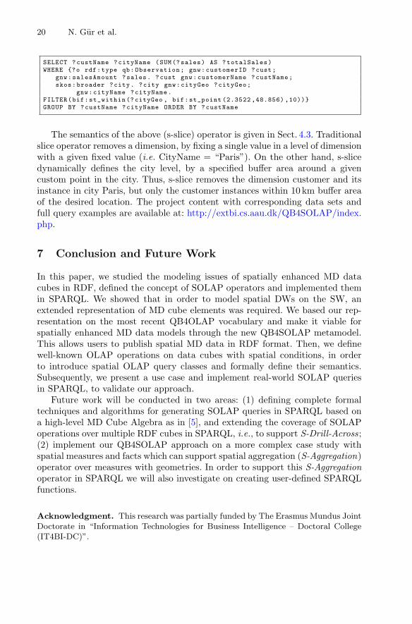
Query 2 (S-Slice): Total sales to the customers located in the city within a10 km buffer area from a given point.

12 SPARQL endpoint is available at: http://extbi.ulb.ac.be:8890/sparql.

20 N. Gur et al.

SELECT ?custName ?cityName (SUM(?sales) AS ?totalSales)WHERE {?o rdf:type qb:Observation; gnw:customerID ?cust;

gnw:salesAmount ?sales. ?cust gnw:customerName ?custName;skos:broader ?city. ?city gnw:cityGeo ?cityGeo;

gnw:cityName ?cityName.FILTER(bif:st_within (?cityGeo , bif:st_point (2.3522 ,48.856) ,10))}GROUP BY ?custName ?cityName ORDER BY ?custName

The semantics of the above (s-slice) operator is given in Sect. 4.3. Traditionalslice operator removes a dimension, by fixing a single value in a level of dimensionwith a given fixed value (i.e. CityName = “Paris”). On the other hand, s-slicedynamically defines the city level, by a specified buffer area around a givencustom point in the city. Thus, s-slice removes the dimension customer and itsinstance in city Paris, but only the customer instances within 10 km buffer areaof the desired location. The project content with corresponding data sets andfull query examples are available at: http://extbi.cs.aau.dk/QB4SOLAP/index.php.

7 Conclusion and Future Work

In this paper, we studied the modeling issues of spatially enhanced MD datacubes in RDF, defined the concept of SOLAP operators and implemented themin SPARQL. We showed that in order to model spatial DWs on the SW, anextended representation of MD cube elements was required. We based our rep-resentation on the most recent QB4OLAP vocabulary and make it viable forspatially enhanced MD data models through the new QB4SOLAP metamodel.This allows users to publish spatial MD data in RDF format. Then, we definewell-known OLAP operations on data cubes with spatial conditions, in orderto introduce spatial OLAP query classes and formally define their semantics.Subsequently, we present a use case and implement real-world SOLAP queriesin SPARQL, to validate our approach.

Future work will be conducted in two areas: (1) defining complete formaltechniques and algorithms for generating SOLAP queries in SPARQL based ona high-level MD Cube Algebra as in [5], and extending the coverage of SOLAPoperations over multiple RDF cubes in SPARQL, i.e., to support S-Drill-Across;(2) implement our QB4SOLAP approach on a more complex case study withspatial measures and facts which can support spatial aggregation (S-Aggregation)operator over measures with geometries. In order to support this S-Aggregationoperator in SPARQL we will also investigate on creating user-defined SPARQLfunctions.

Acknowledgment. This research was partially funded by The Erasmus Mundus JointDoctorate in “Information Technologies for Business Intelligence – Doctoral College(IT4BI-DC)”.

Modeling and Querying Spatial Data Warehouses on the Semantic Web 21

References

1. Abello, A., Romero, O., Pedersen, T.B., Berlanga Llavori, R., Nebot, V.,Aramburu, M., Simitsis, A.: Using semantic web technologies for exploratoryOLAP: a survey. TKDE 99, 571–588 (2014)

2. Andersen, A.B., Gur, N., Hose, K., Jakobsen, K.A., Pedersen, T.B.: Publish-ing danish agricultural government data as semantic web data. In: Supnithi, T.,Yamaguchi, T., Pan, J.Z., Wuwongse, V., Buranarach, M. (eds.) JIST 2014. LNCS,vol. 8943, pp. 178–186. Springer, Heidelberg (2015)

3. Battle, R., Kolas, D.: GeoSPARQL: enabling a geospatial SW. Seman. Web 3(4),355–370 (2012)

4. Bimonte, S., Johany, F., Lardon, S.: A first framework for mutually enhancingchorem and spatial OLAP systems. In: DATA (2015)

5. Ciferri, C., Gomez, L., Schneider, M., Vaisman, A.A., Zimanyi, E.: Cube algebra:a generic user-centric model and query language for OLAP cubes. IJDWM 9(2),39–65 (2013)

6. Cyganiak, R., Reynolds, D., Tennison, J.: The RDF Data Cube Vocabulary. W3C(2014)

7. Deb Nath, R.P., Hose, K., Pedersen, T.B.: Towards a programmable seman-tic extract-transform-load framework for semantic data warehouses. In: DOLAP(2015)

8. Diamantini, C., Potena, D.: Semantic enrichment of strategic datacubes. In:DOLAP (2008)

9. Etcheverry, L., Vaisman, A., Zimanyi, E.: Modeling and querying data warehouseson the semantic web using QB4OLAP. In: Bellatreche, L., Mohania, M.K. (eds.)DaWaK 2014. LNCS, vol. 8646, pp. 45–56. Springer, Heidelberg (2014)

10. Gomez, L.I., Gomez, S.A., Vaisman, A.A.: A generic data model and query lan-guage for spatiotemporal OLAP cube analysis. In: EDBT (2012)

11. Han, J., Stefanovic, N., Koperski, K.: Selective materialization: an efficient methodfor spatial data cube construction. In: Wu, X., Kotagiri, R., Korb, K.B. (eds.)PAKDD 1998. LNCS, vol. 1394, pp. 144–158. Springer, Heidelberg (1998)

12. Kampgen, B., O’Riain, S., Harth, A.: Interacting with statistical linked datavia OLAP operations. In: Simperl, E., Norton, B., Mladenic, D., Valle, E.D.,Fundulaki, I., Passant, A., Troncy, R. (eds.) ESWC 2012. LNCS, vol. 7540, pp.87–101. Springer, Heidelberg (2012)

13. Koubarakis, M., Karpathiotakis, M., Kyzirakos, K., Nikolaou, C., Sioutis, M.: Datamodels and query languages for linked geospatial data. In: Eiter, T., Krennwallner,T. (eds.) Reasoning Web 2012. LNCS, vol. 7487, pp. 290–328. Springer, Heidelberg(2012)

14. Kyzirakos, K., Karpathiotakis, M., Koubarakis, M.: Strabon: a semantic geospatialDBMS. In: Cudre-Mauroux, P., et al. (eds.) ISWC 2012, Part I. LNCS, vol. 7649,pp. 295–311. Springer, Heidelberg (2012)

15. Le Grange, J.J., Lehmann, J., Athanasiou, S., Rojas, A.G., et al.: The GeoKnowgenerator: managing geospatial data in the linked data web. In: Linking GeospatialData (2014)

16. Malinowski, E., Zimanyi, E.: Advanced Data Warehouse Design: FromConventional to Spatial and Temporal Applications. Springer, Heidelberg (2008)

17. Nebot, V., Berlanga, R., Perez, J.M., Aramburu, M.J., Pedersen, T.B.:Multidimensional integrated ontologies: a framework for designing semantic datawarehouses. In: Spaccapietra, S., Zimanyi, E., Song, I.-Y. (eds.) Journal on DataSemantics XIII. LNCS, vol. 5530, pp. 1–36. Springer, Heidelberg (2009)

22 N. Gur et al.

18. Revesz, P.: Introduction to Databases: From Biological to Spatio-Temporal.Springer, Heidelberg (2010)

19. Stadler, C., Lehmann, J., Hffner, K., Auer, S.: Linkedgeodata: a core for a web ofspatial open data. Semant. Web 3(4), 333–354 (2012)

20. Vaisman, A.A., Zimanyi, E.: A multidimensional model representing continuousfields in spatial data warehouses. In: ACM SIGSPATIAL (2009)