Modeling and Querying Multidimensional Bitemporal Data ... · Modeling and Querying Multidimensional Bitemporal Data Warehouses . Canan Eren . Atay. 1, Gözde . Alp. 2 * 1. D. okuz

Modeling and Querying Multidimensional Bitemporal Data Warehouses

Canan Eren Atay1, Gözde Alp2*

1 Dokuz Eylul University, Tinaztepe Campus, Computer Engineering Department, Buca, Izmir, Turkey. 2 Marmara University, Goztepe Campus, Computer Engineering Department, Kadıkoy, Istanbul, Turkey. * Corresponding author. Email: [email protected] Manuscript submitted November 3, 2014; accepted May 28, 2015. doi: 10.17706/ijcce.2016.5.2.110-119

Abstract: Data warehouses have been considered to be the key aspect of success for any Decision Support

System (DSS). Temporal database research has produced important results in this field. Data warehouses

store historical data, and therefore could clearly benefit from the research on temporal databases. Temporal

data warehouses join the two fields of temporal databases and data warehouse research. This paper

introduces a bitemporal data warehouse model that both valid time and transaction time are attached to

attributes. Data warehouse objects and cubes are created with multidimensional bitemporal relational

database. Performance of available well-known relational database and bitemporal extension for data

warehouse is evaluated and compared in terms of execution time and disk space consumption with the set

of queries.

Key words: Attribute time stamping, big data, bitemporal databases, data warehouse, OLAP.

1. Introduction

Big data is one of the most popular research topics in recent years. Technology is an indispensable part of

people's life. Communication, shopping, transaction habits have changed. When surfing on social web sides

a lot of data is left unconsciously. This data is processed and utilized to make recommendations or utilized

to increase profits.

Data warehousing has been an active research area, with the purpose to access historical data. A data

warehouse is “a collection of subject-oriented, integrated, non-volatile, and time-variant data to support

management’s decisions” [1]. It attempts to obtain specially prepared data in an easy and quick way. This

type of data is used in management reports, various business queries, decision support systems, manager

information systems, and data mining applications all by linking the various silos of data that are

distributed throughout an organization [2]. From the early nineties, data warehouses have been considered

to be the key aspect of success for any Decision Support System (DSS). Undoubtedly, the user of a data

warehouse needs to be confident that the data in that warehouse is timely, accurate, and complete.

Non-volatile and time-variant data features of data warehousing suggest that it should allow changes to

data values without overwriting existing values.

OLAP (online analytical processing) is an outgrowth of the need to reach live, real, and prepared data. It is

possible to perform future analysis with OLAP reports with good statistical reliability. The data in an OLAP

cube is updated and worked out again at certain times of the day. Totals, averages, and the other operations

International Journal of Computer and Communication Engineering

110 Volume 5, Number 2, March 2016

are calculated over with this new live data. When a report is presented via OLAP cubes, there is no

calculation performed when reporting. All the calculated values are generally stored in the OLAP cubes as

before. The only processing consists of calling the report and then displaying it. Versioning and dynamic

update of OLAP dimensions are studied in [3], [4]. Typical OLAP operations include rollup (increasing the

level of aggregation) and drill-down (decreasing the level of aggregation or increasing detail) along one or

more dimension hierarchies, slice_and_dice (selection and projection), and pivot (re-orienting the

multidimensional view of data) [5], [6].

Temporal database research has produced important results in this field. A temporal database may

capture either the history of the relevant objects and their attributes (known as valid time), or the history of

the database activity (known as transaction time). A valid time is necessarily used in order to model the

time-varying states of an object and its attributes. These states may be in the past, present, or even in the

future. A transaction time denotes the timestamp of any change as it is recorded in the database. It may not

extend beyond the current time and is system generated. Having only a valid time captures the history of an

object, but it does not preserve the history of any retroactive or post active changes. Having only the

transaction time, one does not preserve the historical or future data, i.e., the validity period of data values.

However, bitemporal databases can model our changing knowledge of a changing world, and hence

associate data values with facts, and thus specify when the facts were valid, thereby providing a complete

history of the data values and their changes [7].

Data warehouses store historical data, and therefore could clearly benefit from the research on temporal

databases. Temporal data warehouses join the two fields of temporal databases and data warehouse

research, in order to manage time-varying multidimensional data. There are research projects that have

already combined data warehouses and temporal databases. A multidimensional model is presented by

Malinowski and Zimanyi [8] that allows time varying and time-invariant examples. Martin and Abello [9]

introduced detailed information about differences and similarities between data warehouse and temporal

database. Eder, Koncilia and Morzy [10] implemented temporal data warehouse model with two different

approach. One of them is called direct approach which uses a query analyzer and result analyzer to obtain

the result of each. Other one is called indirect approach that generates a data mart for a particular structure

version and transforms the data from all other structure versions into this data mart using the given

specication of transformation functions. While the direct approach offers greater flexibility, the indirect

approach is superior in terms of response time, once the data mart has been generated. Janet , Ram´ırez and

Guerrero [11] present a model for changing, adding, removing dimensions of data warehouse cube with no

harmful affect to current applications as well as a query language to manage multidimensional schemas.

Combi, Oliboni and Pozzi [12] present a graph-based model for temporal semi structured data warehouses

also a query language to get required information usefully.

In this paper, we propose a bitemporal extension for data warehouse and OLAP applications in which

both valid time and transaction time are attached to attributes. There are research projects that have

already combined data warehouses and temporal databases. Nonetheless, all of them considered the tuple

time-stamped temporal database approach. To the best of our knowledge, the combination of data

warehousing and attribute time stamping has not been studied before.

The rest of the paper is organized as follows. Section 2 outlines bitemporal databases and common two

time stamping approaches. In Section 3, brief information outlined about data warehouses. Section 4

presents proposed model for bitemporal data warehouses and implementation details. In Section 5 we

present sample queries and test results for the empirical study. Section 6 presents our conclusion and plans

for future work.



2. Bitemporal Databases

Historical database offers temporal knowledge about objects but do not contain system modifications.

Transaction database offers system changes but do not contain temporal information about objects.

Historical and transactional databases must be combined to have complete information about objects.

Bitemporal database covers both these requirements. In this manner, bitemporal databases demonstrate

real world’s data according to real time [13]-[16].

There are two common approaches as to how temporal databases can be implemented: 1) tuple

time-stamping, which uses first normal-form (1NF) relations, and 2) attribute-value time-stamping, which

requires non-first normal-form (N1NF) relations. In the case of tuple time-stamping, a separate relation is

required for each time dependent attribute unless they change simultaneously. Non-time-varying attributes

are grouped into a different relation. A relation scheme is augmented with two (four) time attributes to

designate the time reference of its tuples. Tuple time stamping uses all of the advantages of traditional

relational databases. However, each time varying attribute should be in a separate relation, which results in

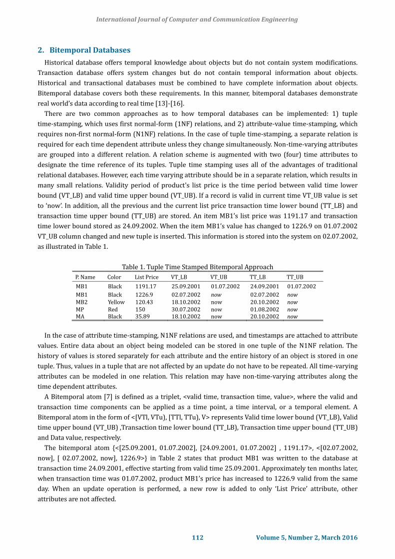
many small relations. Validity period of product's list price is the time period between valid time lower

bound (VT_LB) and valid time upper bound (VT_UB). If a record is valid in current time VT_UB value is set

to ‘now’. In addition, all the previous and the current list price transaction time lower bound (TT_LB) and

transaction time upper bound (TT_UB) are stored. An item MB1’s list price was 1191.17 and transaction

time lower bound stored as 24.09.2002. When the item MB1’s value has changed to 1226.9 on 01.07.2002

VT_UB column changed and new tuple is inserted. This information is stored into the system on 02.07.2002,

as illustrated in Table 1.

Table 1. Tuple Time Stamped Bitemporal Approach

P. Name Color List Price VT_LB VT_UB TT_LB TT_UB

MB1 Black 1191.17 25.09.2001 01.07.2002 24.09.2001 01.07.2002

MB1 Black 1226.9 02.07.2002 now 02.07.2002 now MB2 Yellow 120.43 18.10.2002 now 20.10.2002 now MP Red 150 30.07.2002 now 01.08.2002 now MA Black 35.89 18.10.2002 now 20.10.2002 now

In the case of attribute time-stamping, N1NF relations are used, and timestamps are attached to attribute

values. Entire data about an object being modeled can be stored in one tuple of the N1NF relation. The

history of values is stored separately for each attribute and the entire history of an object is stored in one

tuple. Thus, values in a tuple that are not affected by an update do not have to be repeated. All time-varying

attributes can be modeled in one relation. This relation may have non-time-varying attributes along the

time dependent attributes.

A Bitemporal atom [7] is defined as a triplet, <valid time, transaction time, value>, where the valid and

transaction time components can be applied as a time point, a time interval, or a temporal element. A

Bitemporal atom in the form of <[VTl, VTu), [TTl, TTu), V> represents Valid time lower bound (VT_LB), Valid

time upper bound (VT_UB) ,Transaction time lower bound (TT_LB), Transaction time upper bound (TT_UB)

and Data value, respectively.

The bitemporal atom {<[25.09.2001, 01.07.2002], [24.09.2001, 01.07.2002] , 1191.17>, <[02.07.2002,

now], [ 02.07.2002, now], 1226.9>} in Table 2 states that product MB1 was written to the database at

transaction time 24.09.2001, effective starting from valid time 25.09.2001. Approximately ten months later,

when transaction time was 01.07.2002, product MB1’s price has increased to 1226.9 valid from the same

day. When an update operation is performed, a new row is added to only ‘List Price’ attribute, other

attributes are not affected.



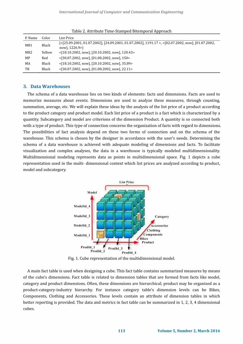
Table 2. Attribute Time-Stamped Bitemporal Approach

P. Name Color List Price

MB1 Black {<[25.09.2001, 01.07.2002], [24.09.2001, 01.07.2002], 1191.17 >, <[02.07.2002, now], [01.07.2002,

now], 1226.9>}

MB2 Yellow <[18.10.2002, now], [20.10.2002, now], 120.43>

MP Red <[30.07.2002, now], [01.08.2002, now], 150>

MA Black <[18.10.2002, now], [20.10.2002, now], 35.89>

TR Black <[30.07.2002, now], [01.08.2002, now], 22.11>

3. Data Warehouses

The schema of a data warehouse lies on two kinds of elements: facts and dimensions. Facts are used to

memorize measures about events. Dimensions are used to analyze these measures, through counting,

summation, average, etc. We will explain these ideas by the analysis of the list price of a product according

to the product category and product model. Each list price of a product is a fact which is characterized by a

quantity. Subcategory and model are criterions of the dimension Product. A quantity is so connected both

with a type of product. This type of connection concerns the organization of facts with regard to dimensions.

The possibilities of fact analysis depend on these two forms of connection and on the schema of the

warehouse. This schema is chosen by the designer in accordance with the user’s needs. Determining the

schema of a data warehouse is achieved with adequate modeling of dimensions and facts. To facilitate

visualization and complex analyses, the data in a warehouse is typically modeled multidimensionality.

Multidimensional modeling represents data as points in multidimensional space. Fig. 1 depicts a cube

representation used in the multidimensional context which list prices are analyzed according to product,

model and subcategory.

Fig. 1. Cube representation of the multidimensional model.

A main fact table is used when designing a cube. This fact table contains summarized measures by means

of the cube's dimensions. Fact table is related to dimension tables that are formed from facts like model,

category and product dimensions. Often, these dimensions are hierarchical; product may be organized as a

product-category-industry hierarchy. For instance category table's dimension levels can be Bikes,

Components, Clothing and Accessories. These levels contain an attribute of dimension tables in which

better reporting is provided. The data and metrics in fact table can be summarized in 1, 2, 3, 4 dimensional

cubes.



4. Bitemporal Data Warehouse Model and Implementation

We obtained data from the Microsoft Adventure Works (AW) database that is available to the public for

research and experiment purposes. Although said database has five modules, we only applied our method

to the Production module. We reformed the Production module schema as nested attribute time-stamped

bitemporal schema. According to the AW structure, some tables are built in their related tables as nested

tables to avoid redundancy. Whereas there are 25 tables in the AW database Product module, our method

generated 15 tables.

The type system facilities of object-relational databases allow us to define a bitemporal atom as a

structured user defined type as seen in Fig. 2. Removing or retrieving a component such as the transaction

time lower and/or upper bound is allowed and used in the query expressions. Once the user defined type is

defined, it can be used in SQL statements where other built-in types are used.

CREATE TYPE BT_NUMBER AS (

VT_LB DATE,

VT_UB DATE,

TT_LB DATE,

TT_UB DATE,

VALUE NUMBER);

Fig. 2. User defined type definition of a bitemporal atom BT_NUMBER.

CREATE TYPE LISTPRICE AS TABLE OF BT_NUMBER;

CREATE TYPE PRODUCTSELL AS TABLE OF

BT_NUMBER;

CREATE TYPE PRODUCTCOST AS TABLE OF

BT_NUMBER;

Fig. 3. The tuples of LISTPRICE are as nested table, BT_NUMBER.

User Defined Types can be declared to be the “data type” of an entire table such that the table’s attributes

are defined by the User Defined Type. By in-lining the repeated fields in the table, the reliance on creating

another table with its own structure and indexes is removed in collection type tables. Data manipulation

operations such as select, insert, and delete can be applied similar to ordinary tables. A nested table is an

unordered collection of elements of the same data type. It can have any number of elements; no maximum

number is specified in the definition of the table.

A tuple in a nested bitemporal relation is an instance of the structured type on which the table is defined.

It gives the instance a unique identity. Having a set of identical User Defined Types in a single tuple actually

simulates the attribute time-stamping approach with a single-attribute table for each object’s time related

attributes.

The AW database table structure and temporal construction is analyzed and re-designed. The SQL

statement in Fig. 3 shows that LISTPRICE, PRODUCTSELL, and PRODUCTCOST are attribute time-stamped

bitemporal relations. These bitemporal tables are single-attribute tables with a type of BT_NUMBER. The

table can have as many tuples as required to represent bitemporal atoms.

Conceptual models allow describing the requirements of an application in terms that are as close as

possible to users’ perception. Thus, they facilitate the communication between users and designers since

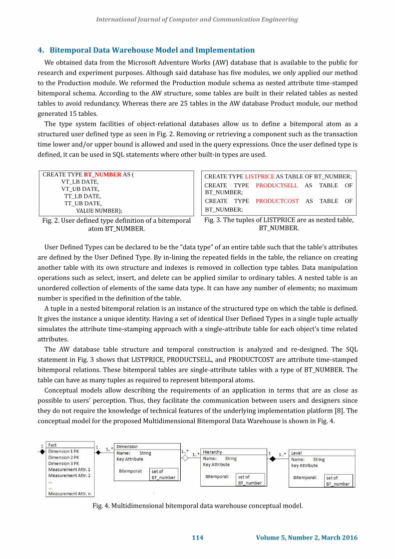
they do not require the knowledge of technical features of the underlying implementation platform [8]. The

conceptual model for the proposed Multidimensional Bitemporal Data Warehouse is shown in Fig. 4.

Fig. 4. Multidimensional bitemporal data warehouse conceptual model.



A fact table is connected to three or more dimension tables. A dimension is composed of one or more

hierarchies, whereas each hierarchy belongs to only one dimension. A hierarchy contains one or more

related levels that can be shared between different hierarchies. Levels have a key and descriptive attributes.

Attributes have a name and a type, which must be a data type, i.e., integer, real, string, etc. Bitemporal

support for levels and for attributes is captured by the multivalued attribute of type BT_NUMBER. A

hierarchy is temporal if it has at least one temporal level. A dimension is temporal if it has at least one

temporal hierarchy. Levels, hierarchies, and dimensions can have many time-varying attributes stored as

nested tables.

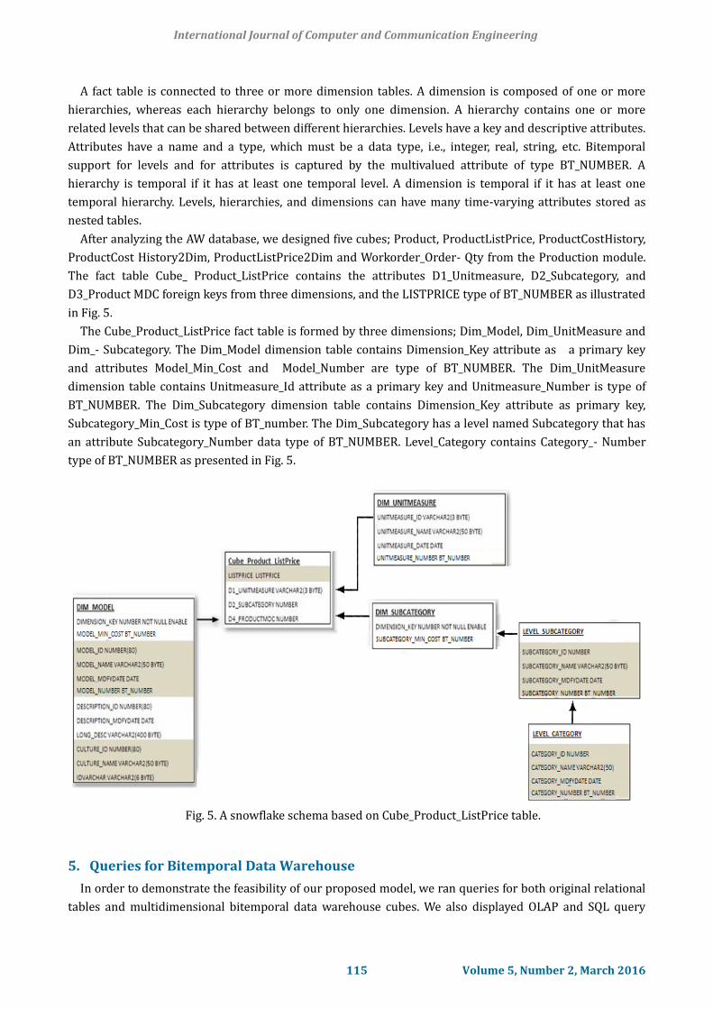
After analyzing the AW database, we designed five cubes; Product, ProductListPrice, ProductCostHistory,

ProductCost History2Dim, ProductListPrice2Dim and Workorder_Order- Qty from the Production module.

The fact table Cube_ Product_ListPrice contains the attributes D1_Unitmeasure, D2_Subcategory, and

D3_Product MDC foreign keys from three dimensions, and the LISTPRICE type of BT_NUMBER as illustrated

in Fig. 5.

The Cube_Product_ListPrice fact table is formed by three dimensions; Dim_Model, Dim_UnitMeasure and

Dim_- Subcategory. The Dim_Model dimension table contains Dimension_Key attribute as a primary key

and attributes Model_Min_Cost and Model_Number are type of BT_NUMBER. The Dim_UnitMeasure

dimension table contains Unitmeasure_Id attribute as a primary key and Unitmeasure_Number is type of

BT_NUMBER. The Dim_Subcategory dimension table contains Dimension_Key attribute as primary key,

Subcategory_Min_Cost is type of BT_number. The Dim_Subcategory has a level named Subcategory that has

an attribute Subcategory_Number data type of BT_NUMBER. Level_Category contains Category_- Number

type of BT_NUMBER as presented in Fig. 5.

Fig. 5. A snowflake schema based on Cube_Product_ListPrice table.

5. Queries for Bitemporal Data Warehouse

In order to demonstrate the feasibility of our proposed model, we ran queries for both original relational

tables and multidimensional bitemporal data warehouse cubes. We also displayed OLAP and SQL query



codes written for both approaches as illustrated in Tables 3 to 6. Each query was run six times and the

average value is selected. Fig. 6 is the result of query times for all queries.

5.1. Query 1: What Is the Average List Price of Bikes According to Years?

The Query 1 is written for both the multidimensional bitemporal data warehouse cubes and the relational

database tables as illustrated in Table 3. The multidimensional bitemporal data warehouse script retrieves

result from CUBEPRODUCTLISTPRICE table and contains one nested select statement that retrieves data

from DIM_SUBCATE- GORY dimension table. The relational database script retrieves data from

PRODUCTION.PRODUCTLISTPRICE- HISTORY table and contains three nested select queries, each of these

nested select queries retrieve data from separate tables.

Table 3. Query 1 with Multidimensional Bitemporal and Relational Databases Multidimensional Bitemporal: SELECT AVG(LISTPRICE.VALUE), LISTPRICE .VT_LB, LISTPRICE.VT_UB, LISTPRICE.TT_LB FROM CUBEPRODUCTLISTPRICE WHERE DIM_SUBCATEGORY_KEY IN (SELECT DIMENSION_KEY FROM DIM_SUBCATEGORY WHERE CATEGORY_NAME='BIKES') GROUP BY VT_LB ,TT_LB; Relational: SELECT AVG( LISTPRICE) , STARTDATE, ENDDATE, MODIFIEDDATE FROM PRODUCTION.PRODUCTLISTPRICEHISTORYWHERE PRODUCTID IN ( SELECT PRODUCTID FROM PRODUCTION.PRODUCT WHERE PRODUCTSUBCATEGORYID IN (SELECT PRODUCTSUBCATEGORYID FROM PRODUCTION.PRODUCTSUBCATEGORY WHERE PRODUCTCATEGORYID= (SELECT PRODUCTCATEGORYID FROM PRODUCTION.PRODUCTCATEGORY WHERE NAME='BIKES'))) GROUP BY STARTDATE, MODIFIEDDATE;

5.2. Query 2: What Is the Average List Price of Bikes According to Cultures?

Scripts that give the same result for the Query 2 is written for the multidimensional bitemporal data

warehouse cube tables and the relational database tables as depicted in Table 4 The multidimensional

bitemporal data warehouse script retrieves result from CUBEPRODUCTLISTPRICE cube and DIM_MODEL

dimension tables, associated each other by a where clause. The multidimensional bitemporal data-

warehouse script contains two nested select statements to retrieve data from separate tables. The relational

database script retrieves data from four separate tables, associated each other by five where clauses.

Table 4. Query 2 with Multidimensional Bitemporal and Relational Databases

Multidimensional Bitemporal: SELECT AVG(LISTPRICE) AS AVERAGE_BIKE_PRICE, DIM_MODEL.CULTURE_NAME FROM CUBEPRODUCTLISTPRICE, DIM_MODEL WHERE DIM_MODEL.DIMENSION_KEY= CUBEPRODUCTLISTPRICE.DIM_PRODUCTMDC_KEY AND CUBEPRODUCTLISTPRICE.PRODUCT_ID IN (SELECT PRODUCTID FROM PRODUCT2 WHERE SUBCATEGORYID IN (SELECT SUBCATEGORY_ID FROM DIM_SUBCATEGORY WHERE CATEGORY_NAME='BIKES' )) GROUP BY DIM_MODEL.CULTURE_NAME ORDER BY DIM_MODEL.CULTURE_NAME; Relational:

SELECT AVG( PL.LISTPRICE) AS AVERAGE_BIKE_PRICE, C.NAME FROM PRODUCTION.PRODUCTLISTPRICEHISTORY PL, PRODUCTION.PRODUCTMODEL PM, PRODUCTION.PRODUCT P, PRODUCTION.PRODUCTMODELPRODUCTDESCRIPTIONCULTURE PMDC, PRODUCTION.CULTURE C WHERE P.PRODUCTMODELID=PM.PRODUCTMODELID AND PL.PRODUCTID=P.PRODUCTID AND PM.PRODUCTMODELID=PMDC.PRODUCTMODELID AND PMDC.CULTUREID=C.CULTUREID) AND PL.PRODUCTID IN (SELECT PRODUCTID FROM PRODUCTION.PRODUCT WHERE PRODUCTSUBCATEGORYID IN (SELECT PRODUCTSUBCATEGORYID FROM PRODUCTION.PRODUCTSUBCATEGORY WHERE PRODUCTCATEGORYID= (SELECT PRODUCTCATEGORYID FROM PRODUCTION.PRODUCTCATEGORY WHERE NAME='BIKES'))) GROUP BY C.NAME ORDER BY C.NAME;



5.3. Query 3: What Is the Average List Price of Components According to Cultures and Models?

The Query 3 for the multidimensional bitemporal data warehouse retrieves data from

CUBEPRODUCTLISTPRICE cube and DIM_MODEL dimension tables. It contains two nested select

statements. The relational database code retrieves data from four separate tables that contains three nested

select queries as seen in Table 5.

Table 5. Query 3 with Dimensional and Relational Databases

Multidimensional Bitemporal: SELECT AVG(LISTPRICE), DIM_MODEL.CULTURE_NAME, DIM_MODEL.MODEL_NAME FROM CUBEPRODUCTLISTPRICE, DIM_MODEL WHERE DIM_MODEL.DIMENSION_KEY= CUBEPRODUCTLISTPRICE.DIM_PRODUCTMDC_KEY AND CUBEPRODUCTLISTPRICE.PRODUCT_ID IN (SELECT PRODUCTID FROM PRODUCT2 WHERE SUBCATEGORYID IN (SELECT SUBCATEGORY_ID FROM DIM_SUBCATEGORY WHERE CATEGORY_NAME='COMPONENTS' )) GROUP BY DIM_MODEL.MODEL_NAME, DIM_MODEL.CULTURE_NAME ORDER BY DIM_MODEL. MODEL_NAME, DIM_MODEL.CULTURE_NAME;

Relational: SELECT AVG( PL.LISTPRICE), C.NAME , PM.NAME FROM PRODU CTION.PRODUCTLISTPRICEHISTORY PL, PRODUCTION.PRODUCTMODEL PM, PRODUCTION.PRODUCT P, PRODUCTION.PRODUCTMODELPRODUCTDESCRIPTIONCULTURE PMDC, PRODUCTION.CULTURE C WHERE P.PRODUCTMODELID= PM.PRODUCTMODELID AND PL.PRODUCTID=P.PRODUCTID AND PM.PRODUCTMODELID=PMDC.PRODUCTMODELID AND PMDC.CULTUREID=C.CULTUREID AND PL.PRODUCTID=P.PRODUCTID AND PL.PRODUCTID IN (SELECT PRODUCTID FROM PRODUCTION.PRODUCT WHERE PRODUCTSUBCATEGORYID IN(SELECT PRODUCTSUBCATEGORYID FROM PRODUCTION.PRODUCTSUBCATEGORY WHERE PRODUCTCATEGORYID= ( SELECT PRODUCTCATEGORYID FROM PRODUCTION.PRODUCTCATEGORY WHERE NAME='COMPONENTS'))) GROUP BY C.NAME, PM.NAME ORDER BY C.NAME, PM.NAME;

5.4. Query 4: List of All Work Orders in Ordered by According to Category, Subcategory and Product Name.

The multidimensional bitemporal data warehouse query retrieves data from

CUBE_WORKORDER_ORDERQTY cube and DIM_PRODUCT dimension tables associated each other by a

where clause. The relational database query retrieves data from four separate tables as illustrated in Table

6.

Table 6. Query 4 with Multidimensional Bitemporal and Relational Databases

Multidimensional Bitemporal: SELECT CUBE_WORKORDER_ORDERQTY.VT_LB, CUBE_WORKORDER_ORDERQTY.VT_UB, CUBE_WORKORDER_ORDERQTY.TT_LB, CUBE_WORKORDER_ORDERQTY.TT_UB, CUBE_WORKORDER_ORDERQTY.VALUE ORDERQTY, DIM_PRODUCT.CATEGORY_NAME, DIM_PRODUCT.SUBCATEGORY_NAME, DIM_PRODUCT.PRODUCT_NAME FROM CUBE_WORKORDER_ORDERQTY, DIM_PRODUCT WHERE DIM_PRODUCT.DIMENSION_KEY= CUBE_WORKORDER_ORDERQTY.DIM_PRODUCT_KEY ORDER BY DIM_PRODUCT.CATEGORY_NAME, DIM_PRODUCT.SUBCATEGORY_NAME, DIM_PRODUCT.PRODUCT_NAME;

Relational: SELECT WO.STARTDATE, WO.ENDDATE , WO.MODIFIEDDATE, WO.MODIFIEDDATE, WO.ORDERQTY, PS.NAME, PC.NAME, P.NAME FROM PRODUCTION.WORKORDER WO, PRODUCTION.PRODUCT P, PRODUCTION.PRODUCTSUBCATEGORY PS, PRODUCTION.PRODUCTCATEGORY PC WHERE P.PRODUCTID=WO.PRODUCTID AND P.PRODUCTSUBCATEGORYID=PS.PRODUCTSUBCATEGORYID AND PS.PRODUCTCATEGORYID=PC.PRODUCTCATEGORYID ORDER BY PS.NAME, PC.NAME,P.NAME



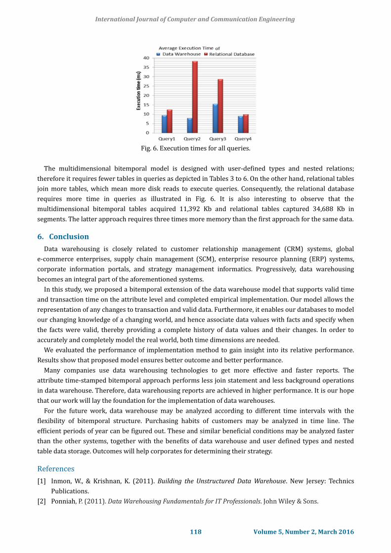
Fig. 6. Execution times for all queries.

The multidimensional bitemporal model is designed with user-defined types and nested relations;

therefore it requires fewer tables in queries as depicted in Tables 3 to 6. On the other hand, relational tables

join more tables, which mean more disk reads to execute queries. Consequently, the relational database

requires more time in queries as illustrated in Fig. 6. It is also interesting to observe that the

multidimensional bitemporal tables acquired 11,392 Kb and relational tables captured 34,688 Kb in

segments. The latter approach requires three times more memory than the first approach for the same data.

6. Conclusion

Data warehousing is closely related to customer relationship management (CRM) systems, global

e-commerce enterprises, supply chain management (SCM), enterprise resource planning (ERP) systems,

corporate information portals, and strategy management informatics. Progressively, data warehousing

becomes an integral part of the aforementioned systems.

In this study, we proposed a bitemporal extension of the data warehouse model that supports valid time

and transaction time on the attribute level and completed empirical implementation. Our model allows the

representation of any changes to transaction and valid data. Furthermore, it enables our databases to model

our changing knowledge of a changing world, and hence associate data values with facts and specify when

the facts were valid, thereby providing a complete history of data values and their changes. In order to

accurately and completely model the real world, both time dimensions are needed.

We evaluated the performance of implementation method to gain insight into its relative performance.

Results show that proposed model ensures better outcome and better performance.

Many companies use data warehousing technologies to get more effective and faster reports. The

attribute time-stamped bitemporal approach performs less join statement and less background operations

in data warehouse. Therefore, data warehousing reports are achieved in higher performance. It is our hope

that our work will lay the foundation for the implementation of data warehouses.

For the future work, data warehouse may be analyzed according to different time intervals with the

flexibility of bitemporal structure. Purchasing habits of customers may be analyzed in time line. The

efficient periods of year can be figured out. These and similar beneficial conditions may be analyzed faster

than the other systems, together with the benefits of data warehouse and user defined types and nested

table data storage. Outcomes will help corporates for determining their strategy.

References

[1] Inmon, W., & Krishnan, K. (2011). Building the Unstructured Data Warehouse. New Jersey: Technics

Publications.

[2] Ponniah, P. (2011). Data Warehousing Fundamentals for IT Professionals. John Wiley & Sons.



[3] Subotić, D., Poščić, P., & Jovanović, V. (2014). Data warehouse schema evolution: State of the art. Centra,

European Conference on Information and Intelligent Systems (pp. 18-23). Varaždin, Croatia.

[4] Ravat, F., & Teste, O. (2006). Supporting data changes in multidimensional data warehouses.

International Review on Computers and Software (pp. 251-259).

[5] Ceci, M., Cuzzocrea, A., & Malerba, D. (2013). Effectively and efficiently supporting roll-up and

drill-down OLAP operations over continuous dimensions via hierarchical clustering. Journal of

Intelligent Information Systems, 1–25.

[6] Wrembel, R. (November 2010). A survey on managing the evolution of data warehouses. International

Journal of Database Management Systems, 2(4).

[7] Atay, C. E., & Tansel, A. U. (2009). Bitemporal databases: Modeling and implementation. Germany: VDM

Publishing.

[8] Malinowski, E., & Zimanyi, E. (2006). A conceptual solution for representing time in data warehouse

dimensions. Proceedings of 3rd Asia-Pacific Conference on Conceptual Modeling (pp. 45–54).

[9] Abelló, A., & Martín, C. (2003). The data warehouse: An object-oriented temporal database. Proceedings

of VIII Jornadas Ingeniería del Software y Bases de Datos (pp. 675-684).

[10] Eder, J., Koncilia, C., & Morzy, T. (2001). A model for a temporal data warehouse. Proceedings of OES-SEO

Workshop (pp. 48-54).

[11] Janet, E., Ram´ırez, R., & Guerrero, E. B. (2006). A model and language for bitemporal schema

versioning in data warehouses. Proceedings of IEEE 15th International Conference on Computing (pp.

309-314). Mexico City.

[12] Combi, C., Oliboni, B., & Pozzi, G. (2009). Modeling and querying temporal semistructured data

warehouses. New Trends in Data Warehousing and Data Analysis Annals of Information Systems, 3, 1-25.

[13] Ben-Zvi, J. (1982). The Time Relational Model. PhD dissertation, University of California, Los Angeles.

[14] Porter, L. M. L. (2012). Bitemporal relational databases and methods of manufacturing and use. U.S.

Patent Application, 13, 609-614.

[15] Kaufmann, M., Fischer, P. M., May, N., Tonder, A., & Kossmann, D. (2014). TPC-BiH: A benchmark for

bitemporal databases. Springer International Publishing, 8391, 16-31.

[16] Golfarelli, M., & Rizzi, S. (2011). Temporal data warehousing: Approaches and techniques. In D. Taniar,

& L. Chen (Eds.), Temporal Data Warehousing: Approaches and Techniques (pp. 1-18).

Canan Eren Atay received her BS degree in industrial engineering from Anadolu

University, Eskisehir, Turkey; her MS and PhD degrees in computer science from City

University of New York, New York, USA. Dr. Atay works as an assistant professor in the

Computer Engineering Department of Dokuz Eylul University, Izmir, Turkey. She has

published articles and a book on bitemporal data, bitemporal query languages. Dr. Atay’s

research interests include temporal databases, bitemporal databases, nested relations,

spatial databases, data warehousing, temporal information retrieval, and social media

data.

Gözde Alp received the B.S. degree in computer engineering from Suleyman Demirel

University, Isparta, Turkey, in 2011, and the M.S. degree in computer engineering from

Dokuz Eylul University, Izmir, Turkey in 2013. She is a Ph.D. student and a research

assistant in Marmara University Computer Engineering Department, Istanbul, Turkey.

Her research interests include database systems, optimization, and evolutionary

algorithms.



Documents

Modeling and Querying Multidimensional Bitemporal Data ... · Modeling and Querying Multidimensional Bitemporal Data Warehouses . Canan Eren . Atay. 1, Gözde . Alp. 2 * 1. D. okuz