Chemical Engineering Science 64 (2009) 3668 -- 3682

Contents lists available at ScienceDirect

Chemical Engineering Science

journal homepage: www.e lsev ier .com/ locate /ces

Modeling and control of film porosity in thin film deposition

Gangshi Hua, Gerassimos Orkoulasa, Panagiotis D. Christofidesa,b,∗aDepartment of Chemical and Biomolecular Engineering, University of California, Los Angeles, CA 90095, USAbDepartment of Electrical Engineering, University of California, Los Angeles, CA 90095, USA

A R T I C L E I N F O A B S T R A C T

Article history:Received 17 September 2008Accepted 6 May 2009Available online 14 May 2009

Keywords:Process controlMaterials processingProcess modelingProcess simulationThin filmsModel predictive control

Systematic methodologies are developed for modeling and control of film porosity in thin film deposition.The deposition process is modeled via kinetic Monte Carlo (kMC) simulation on a triangular lattice. Themicroscopic events involve atom adsorption and migration and allow for vacancies and overhangs todevelop. Appropriate definitions of film site occupancy ratio (SOR), i.e., fraction of film sites occupied byparticles over total number of film sites, and its fluctuations are introduced to describe film porosity.Deterministic and stochastic ordinary differential equation (ODE) models are also derived to describe thetime evolution of film SOR and its fluctuation. The coefficients of the ODE models are estimated on thebasis of data obtained from the kMC simulator of the deposition process using least-square methods andtheir dependence on substrate temperature is determined. The developed ODE models are used as thebasis for the design of model predictive control (MPC) algorithms that include penalty on the film SORand its variance to regulate the expected value of film SOR at a desired level and reduce run-to-run fluc-tuations. Simulation results demonstrate the applicability and effectiveness of the proposed film porositymodeling and control methods in the context of the deposition process under consideration.

© 2009 Elsevier Ltd. All rights reserved.

1. Introduction

Currently, there is an increasing need to improve semiconduc-tor manufacturing process operation and yield. This need has arisendue to the increased complexity and density of devices on the wafer,which is the result of increased wafer size and smaller device di-mensions. Within this manufacturing environment, thin film mi-crostructure, including thin film surface roughness and amount ofinternal film defects, has emerged as an important film quality vari-able which strongly influences the electrical and mechanical prop-erties of microelectronic devices. On one hand, surface roughnessof thin films controls the interfacial layer and properties betweentwo successively deposited films. On the other hand, the amount ofinternal defects, usually expressed as film porosity, plays an impor-tant role in determining the thin film microstructure. For example,low-k dielectric films of high porosity are being used in current in-terconnect technologies to meet resistive-capacitive delay goals andminimize cross-talk. However, increased porosity negatively affectsthe mechanical properties of dielectric films, increasing the risk of

∗ Corresponding author at: Department of Chemical and Biomolecular Engineer-ing, University of California, Los Angeles, CA 90095, USA. Tel.: +13107941015;fax: +13102064107.

E-mail address: pdc@seas.ucla.edu (P.D. Christofides).

0009-2509/$ - see front matter © 2009 Elsevier Ltd. All rights reserved.doi:10.1016/j.ces.2009.05.008

thermo-mechanical failures (Kloster et al., 2002). Furthermore, in thecase of gate dielectrics, it is important to reduce thin film porosityas much as possible and eliminate the development of holes closeto the interface.

Most of the previous research efforts on modeling and con-trol of thin film microstructure have focused on regulation of thinfilm surface roughness. This line of research has been motivatedby the development of techniques for on-line surface measure-ment including scanning tunneling microscopy, spectroscopic el-lipsometry techniques and grazing-incidence small angle X-rayscattering. Two fundamental modeling approaches, kinetic MonteCarlo (kMC) methods (Gillespie, 1976; Fichthorn and Weinberg,1991; Shitara et al., 1992; Reese et al., 2001; Christofides et al.,2008) and stochastic differential equation (SDE) models (Edwardsand Wilkinson, 1982; Vvedensky et al., 1993; Cuerno et al., 1995;Lauritsen et al., 1996), have been developed to describe the evo-lution of film microscopic configurations and design feedbackcontrol laws. Specifically, kMC models were initially used to de-velop a methodology for modeling and feedback control of thinfilm surface roughness (Lou and Christofides, 2003a,b). Successfulapplications of this control methodology include surface rough-ness control of: (a) a gallium arsenide (GaAs) deposition process(Lou and Christofides, 2004) and (b) a multi-species depositionprocess with long range interactions (Ni and Christofides, 2005a).Furthermore, a method that couples partial differential equation(PDE) models and kMC models was developed for computationally

G. Hu et al. / Chemical Engineering Science 64 (2009) 3668 -- 3682 3669

efficient multiscale optimization of thin film growth (Varshney andArmaou, 2005). However, kMC models are not available in closed-form and this limitation precludes the use of kMCmodels for system-level analysis and the design and implementation of model-basedfeedback control systems. Therefore, it is desirable to achieve betterclosed-loop performance by designing feedback controllers on thebasis of closed-form process models. Linear deterministic modelswere identified in (Siettos et al., 2003; Armaou et al., 2004; Varshneyand Armaou, 2006) from outputs of kMC simulators and were usedin controller design using linear control theory. Deterministic mod-els are effective in controlling the expected values of macroscopicvariables, which correspond to the first-order statistical moments ofthe microscopic distribution. However, to control higher statisticalmoments of the microscopic distributions, such as the surface rough-ness (the second moment of height distribution on a lattice), deter-ministic models are not sufficient and SDE models may be needed.

SDEs arise naturally in the modeling of surface morphology of ul-tra thin films in a variety of material preparation processes (Edwardsand Wilkinson, 1982; Villain, 1991; Vvedensky et al., 1993; Cuernoet al., 1995; Lauritsen et al., 1996) since they contain the surfacemorphology information and account for the stochastic nature ofthe growth processes. For instance, it has been experimentally veri-fied by atomic force microscopy (AFM) that the Kardar–Parisi–Zhang(KPZ) equation (Kardar et al., 1986) describes satisfactorily the evo-lution of the surface morphology of GaAs thin films (Ballestad et al.,2002; Kan et al., 2004). However, the construction of SDE modelsfrom kMC simulation data or experimental data is a challenging task.Compared to deterministic systems, modeling and identification ofdynamical systems of SDEs have received relatively limited atten-tion. Theoretical foundations on the analysis, parameter optimiza-tion, and optimal stochastic control for linear stochastic ordinarydifferential equation (ODE) systems can be found in the early workby Åstrom (1970). More recently, likelihood-based methods for pa-rameter estimation of stochastic ODE models have been developed(Bohlin and Graebe, 1995; Kristensen et al., 2004). These methodsdetermine the model parameters by solving an optimization prob-lem to maximize a likelihood function or a posterior probabilitydensity function of a given sequence of measurements of a stochasticprocess. Recent results employed statistical moments to reformu-late the parameter estimation problem into one involving deter-ministic differential equations. The stochastic moments include theexpected value and variance/covariance obtained from the data setgenerated by kMC simulations or obtained from experiments. Thus,the issue of parameter estimation of stochastic models could beaddressed by employing parameter estimation techniques for de-terministic systems. Specifically, following this idea, a method forconstruction of linear stochastic PDE models for thin film growthwas developed and used to construct linear stochastic PDE modelsfor thin film deposition processes in two-dimensional lattices (Niand Christofides, 2005b). Systematic identification approaches werealso developed for linear (Lou and Christofides, 2005a) and non-linear (Hu et al., 2008b) stochastic PDEs and applied to sputteringprocesses.

Advanced control methods based on SDEs have been developedto address the need of model-based feedback control of thin filmmicrostructure. Specifically, methods for state feedback control ofsurface roughness based on linear (Lou and Christofides, 2005a,b; Niand Christofides, 2005b) and nonlinear (Lou and Christofides, 2006;Lou et al., 2008) SDE models have been developed. However, statefeedback control assumes full knowledge of the surface morphol-ogy at all times, which may be a restrictive requirement in certainpractical applications. To this end, output feedback control of sur-face roughness was recently developed (Hu et al., 2008a) by incor-porating a Kalman–Bucy type filter, which utilizes information froma finite number of noisy measurements.

In the context of modeling of thin film porosity, kMC modelshave been widely used to model the evolution of porous thin filmsin many deposition processes, such as the molecular beam epi-taxial (MBE) growth of silicon films and copper thin film growth(Wang and Clancy, 1998; Zhang et al., 2004). Both monocrystallineand polycrystalline kMC models have been developed and simu-lated (Levine and Clancy, 2000; Wang and Clancy, 2001). The in-fluence of the macroscopic parameters, i.e., the deposition rate andtemperature, on the porous thin film microstructure has also beeninvestigated using kMC simulators of deposition processes. Despiterecent significant efforts on surface roughness control, a close studyof the existing literature indicates the lack of general and practi-cal methods for addressing the challenging issue of achieving de-sired electrical and mechanical thin film properties by controllingfilm porosity to a desired level and reducing run-to-run porosityvariability.

Motivated by these considerations, the present work focuses onthe development of systematic methodologies for modeling and con-trol of film porosity in thin film deposition processes. Initially, a thinfilm deposition process which involves atom adsorption and migra-tion is introduced and is modeled using a triangular lattice-basedkMC simulator which allows porosity, vacancies and overhangs todevelop and leads to the deposition of a porous film. Subsequently,appropriate definitions of film site occupancy ratio (SOR), i.e., frac-tion of film sites occupied by particles over total number of film sites,and its fluctuation are introduced to describe film porosity. Then,deterministic and stochastic ODE models are derived that describethe time evolution of film SOR and its fluctuation. The coefficients ofthe ODE models are estimated on the basis of data obtained from thekMC simulator of the deposition process using least-square methodsand their dependence on substrate temperature is determined. Thedeveloped ODE models are used as the basis for the design of model-predictive control (MPC) algorithms that include penalty on the filmSOR and its variance to regulate the expected value of film SOR at adesired level and reduce run-to-run fluctuations. Simulation resultsdemonstrate the applicability and effectiveness of the proposed filmporosity modeling and control methods in the context of the depo-sition process under consideration.

2. Thin film deposition process description and modeling

This section is associated with the description of the kMC algo-rithm of a thin film deposition process. Two microscopic processesare considered; atom adsorption and surface migration. Vacanciesand overhangs are allowed in the kMC model to introduce porosityduring the thin film growth. Substrate temperature and depositionrate are the macroscopic parameters which control the depositionprocess.

2.1. On-lattice kinetic Monte Carlo model of film growth

The thin film growth process considered in this work includestwo microscopic processes: an adsorption process, in which particlesare incorporated into the film from the gas phase, and a migrationprocess, in which surface particles move to adjacent sites (Wang andClancy, 1998, 2001; Levine and Clancy, 2000; Yang et al., 1997). Solid-on-solid (SOS) deposition models, in which vacancies and overhangsare forbidden, are frequently used to model thin film deposition pro-cesses (Ni and Christofides, 2005a; Lou and Christofides, 2008) andinvestigate the surface evolution of thin films. However, vacanciesand overhangs must be incorporated in the process model to ac-count for film porosity. Since SOS models are inadequate to modelthe evolution of thin film internal micro-structure, a ballistic depo-sition model is chosen to simulate the evolution of film porosity.

3670 G. Hu et al. / Chemical Engineering Science 64 (2009) 3668 -- 3682

0Gas phase

La

�

Substrate

Particleson lattice

Gas phaseparticles

Substrateparticles

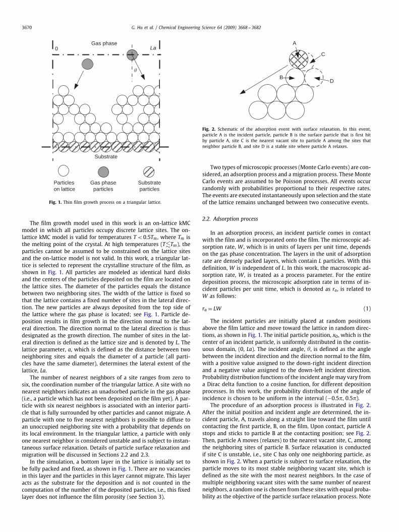
Fig. 1. Thin film growth process on a triangular lattice.

The film growth model used in this work is an on-lattice kMCmodel in which all particles occupy discrete lattice sites. The on-lattice kMC model is valid for temperatures T <0.5Tm, where Tm isthe melting point of the crystal. At high temperatures (T�Tm), theparticles cannot be assumed to be constrained on the lattice sitesand the on-lattice model is not valid. In this work, a triangular lat-tice is selected to represent the crystalline structure of the film, asshown in Fig. 1. All particles are modeled as identical hard disksand the centers of the particles deposited on the film are located onthe lattice sites. The diameter of the particles equals the distancebetween two neighboring sites. The width of the lattice is fixed sothat the lattice contains a fixed number of sites in the lateral direc-tion. The new particles are always deposited from the top side ofthe lattice where the gas phase is located; see Fig. 1. Particle de-position results in film growth in the direction normal to the lat-eral direction. The direction normal to the lateral direction is thusdesignated as the growth direction. The number of sites in the lat-eral direction is defined as the lattice size and is denoted by L. Thelattice parameter, a, which is defined as the distance between twoneighboring sites and equals the diameter of a particle (all parti-cles have the same diameter), determines the lateral extent of thelattice, La.

The number of nearest neighbors of a site ranges from zero tosix, the coordination number of the triangular lattice. A site with nonearest neighbors indicates an unadsorbed particle in the gas phase(i.e., a particle which has not been deposited on the film yet). A par-ticle with six nearest neighbors is associated with an interior parti-cle that is fully surrounded by other particles and cannot migrate. Aparticle with one to five nearest neighbors is possible to diffuse toan unoccupied neighboring site with a probability that depends onits local environment. In the triangular lattice, a particle with onlyone nearest neighbor is considered unstable and is subject to instan-taneous surface relaxation. Details of particle surface relaxation andmigration will be discussed in Sections 2.2 and 2.3.

In the simulation, a bottom layer in the lattice is initially set tobe fully packed and fixed, as shown in Fig. 1. There are no vacanciesin this layer and the particles in this layer cannot migrate. This layeracts as the substrate for the deposition and is not counted in thecomputation of the number of the deposited particles, i.e., this fixedlayer does not influence the film porosity (see Section 3).

A

C

DB

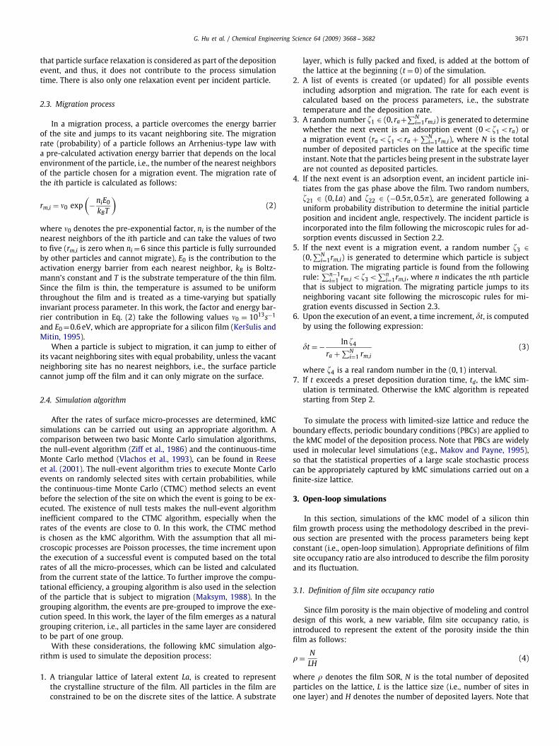
Fig. 2. Schematic of the adsorption event with surface relaxation. In this event,particle A is the incident particle, particle B is the surface particle that is first hitby particle A, site C is the nearest vacant site to particle A among the sites thatneighbor particle B, and site D is a stable site where particle A relaxes.

Two types of microscopic processes (Monte Carlo events) are con-sidered, an adsorption process and a migration process. These MonteCarlo events are assumed to be Poisson processes. All events occurrandomly with probabilities proportional to their respective rates.The events are executed instantaneously upon selection and the stateof the lattice remains unchanged between two consecutive events.

2.2. Adsorption process

In an adsorption process, an incident particle comes in contactwith the film and is incorporated onto the film. The microscopic ad-sorption rate, W , which is in units of layers per unit time, dependson the gas phase concentration. The layers in the unit of adsorptionrate are densely packed layers, which contain L particles. With thisdefinition, W is independent of L. In this work, the macroscopic ad-sorption rate, W , is treated as a process parameter. For the entiredeposition process, the microscopic adsorption rate in terms of in-cident particles per unit time, which is denoted as ra, is related toW as follows:

ra = LW (1)

The incident particles are initially placed at random positionsabove the film lattice and move toward the lattice in random direc-tions, as shown in Fig. 1. The initial particle position, x0, which is thecenter of an incident particle, is uniformly distributed in the contin-uous domain, (0, La). The incident angle, �, is defined as the anglebetween the incident direction and the direction normal to the film,with a positive value assigned to the down-right incident directionand a negative value assigned to the down-left incident direction.Probability distribution functions of the incident anglemay vary froma Dirac delta function to a cosine function, for different depositionprocesses. In this work, the probability distribution of the angle ofincidence is chosen to be uniform in the interval (−0.5�, 0.5�).

The procedure of an adsorption process is illustrated in Fig. 2.After the initial position and incident angle are determined, the in-cident particle, A, travels along a straight line toward the film untilcontacting the first particle, B, on the film. Upon contact, particle Astops and sticks to particle B at the contacting position; see Fig. 2.Then, particle A moves (relaxes) to the nearest vacant site, C, amongthe neighboring sites of particle B. Surface relaxation is conductedif site C is unstable, i.e., site C has only one neighboring particle, asshown in Fig. 2. When a particle is subject to surface relaxation, theparticle moves to its most stable neighboring vacant site, which isdefined as the site with the most nearest neighbors. In the case ofmultiple neighboring vacant sites with the same number of nearestneighbors, a random one is chosen from these sites with equal proba-bility as the objective of the particle surface relaxation process. Note

G. Hu et al. / Chemical Engineering Science 64 (2009) 3668 -- 3682 3671

that particle surface relaxation is considered as part of the depositionevent, and thus, it does not contribute to the process simulationtime. There is also only one relaxation event per incident particle.

2.3. Migration process

In a migration process, a particle overcomes the energy barrierof the site and jumps to its vacant neighboring site. The migrationrate (probability) of a particle follows an Arrhenius-type law witha pre-calculated activation energy barrier that depends on the localenvironment of the particle, i.e., the number of the nearest neighborsof the particle chosen for a migration event. The migration rate ofthe ith particle is calculated as follows:

rm,i = �0 exp(

−niE0kBT

)(2)

where �0 denotes the pre-exponential factor, ni is the number of thenearest neighbors of the ith particle and can take the values of twoto five (rm,i is zero when ni =6 since this particle is fully surroundedby other particles and cannot migrate), E0 is the contribution to theactivation energy barrier from each nearest neighbor, kB is Boltz-mann's constant and T is the substrate temperature of the thin film.Since the film is thin, the temperature is assumed to be uniformthroughout the film and is treated as a time-varying but spatiallyinvariant process parameter. In this work, the factor and energy bar-rier contribution in Eq. (2) take the following values �0 = 1013s−1

and E0 =0.6 eV, which are appropriate for a silicon film (Keršulis andMitin, 1995).

When a particle is subject to migration, it can jump to either ofits vacant neighboring sites with equal probability, unless the vacantneighboring site has no nearest neighbors, i.e., the surface particlecannot jump off the film and it can only migrate on the surface.

2.4. Simulation algorithm

After the rates of surface micro-processes are determined, kMCsimulations can be carried out using an appropriate algorithm. Acomparison between two basic Monte Carlo simulation algorithms,the null-event algorithm (Ziff et al., 1986) and the continuous-timeMonte Carlo method (Vlachos et al., 1993), can be found in Reeseet al. (2001). The null-event algorithm tries to execute Monte Carloevents on randomly selected sites with certain probabilities, whilethe continuous-time Monte Carlo (CTMC) method selects an eventbefore the selection of the site on which the event is going to be ex-ecuted. The existence of null tests makes the null-event algorithminefficient compared to the CTMC algorithm, especially when therates of the events are close to 0. In this work, the CTMC methodis chosen as the kMC algorithm. With the assumption that all mi-croscopic processes are Poisson processes, the time increment uponthe execution of a successful event is computed based on the totalrates of all the micro-processes, which can be listed and calculatedfrom the current state of the lattice. To further improve the compu-tational efficiency, a grouping algorithm is also used in the selectionof the particle that is subject to migration (Maksym, 1988). In thegrouping algorithm, the events are pre-grouped to improve the exe-cution speed. In this work, the layer of the film emerges as a naturalgrouping criterion, i.e., all particles in the same layer are consideredto be part of one group.

With these considerations, the following kMC simulation algo-rithm is used to simulate the deposition process:

1. A triangular lattice of lateral extent La, is created to representthe crystalline structure of the film. All particles in the film areconstrained to be on the discrete sites of the lattice. A substrate

layer, which is fully packed and fixed, is added at the bottom ofthe lattice at the beginning (t = 0) of the simulation.

2. A list of events is created (or updated) for all possible eventsincluding adsorption and migration. The rate for each event iscalculated based on the process parameters, i.e., the substratetemperature and the deposition rate.

3. A random number �1 ∈ (0, ra+∑Ni=1rm,i) is generated to determine

whether the next event is an adsorption event (0< �1<ra) ora migration event (ra < �1<ra + ∑N

i=1rm,i), where N is the totalnumber of deposited particles on the lattice at the specific timeinstant. Note that the particles being present in the substrate layerare not counted as deposited particles.

4. If the next event is an adsorption event, an incident particle ini-tiates from the gas phase above the film. Two random numbers,�21 ∈ (0, La) and �22 ∈ (−0.5�, 0.5�), are generated following auniform probability distribution to determine the initial particleposition and incident angle, respectively. The incident particle isincorporated into the film following the microscopic rules for ad-sorption events discussed in Section 2.2.

5. If the next event is a migration event, a random number �3 ∈(0,∑N

i=1rm,i) is generated to determine which particle is subjectto migration. The migrating particle is found from the followingrule:

∑n−1i=1 rm,i < �3<

∑ni=1rm,i, where n indicates the nth particle

that is subject to migration. The migrating particle jumps to itsneighboring vacant site following the microscopic rules for mi-gration events discussed in Section 2.3.

6. Upon the execution of an event, a time increment, �t, is computedby using the following expression:

�t = − ln �4ra +∑N

i=1 rm,i(3)

where �4 is a real random number in the (0, 1) interval.7. If t exceeds a preset deposition duration time, td, the kMC sim-

ulation is terminated. Otherwise the kMC algorithm is repeatedstarting from Step 2.

To simulate the process with limited-size lattice and reduce theboundary effects, periodic boundary conditions (PBCs) are applied tothe kMC model of the deposition process. Note that PBCs are widelyused in molecular level simulations (e.g., Makov and Payne, 1995),so that the statistical properties of a large scale stochastic processcan be appropriately captured by kMC simulations carried out on afinite-size lattice.

3. Open-loop simulations

In this section, simulations of the kMC model of a silicon thinfilm growth process using the methodology described in the previ-ous section are presented with the process parameters being keptconstant (i.e., open-loop simulation). Appropriate definitions of filmsite occupancy ratio are also introduced to describe the film porosityand its fluctuation.

3.1. Definition of film site occupancy ratio

Since film porosity is the main objective of modeling and controldesign of this work, a new variable, film site occupancy ratio, isintroduced to represent the extent of the porosity inside the thinfilm as follows:

� = NLH

(4)

where � denotes the film SOR, N is the total number of depositedparticles on the lattice, L is the lattice size (i.e., number of sites inone layer) and H denotes the number of deposited layers. Note that

3672 G. Hu et al. / Chemical Engineering Science 64 (2009) 3668 -- 3682

L (sites)

H (l

ayer

s)Fig. 3. Illustration of the definition of film SOR of Eq. (4).

the deposited layers are the layers that contain deposited particlesand do not include the initial substrate layer. The concept of packingdensity, which represents the occupancy ratio of space for a specificpacking method, is not the same as the film SOR defined in Eq. (4),and thus, it cannot be used to characterize the evolution of filmporosity.

Fig. 3 gives an example showing how film SOR is defined. Sinceeach layer contains L sites, the total number of sites in the film isLH. Film SOR is the ratio between the number of deposited particles,N, and the total number of sites, LH. With this definition, film SORranges from 0 to 1. Specifically, � = 1 denotes a film whose sitesare fully occupied and has a flat surface. At the beginning of thedeposition process when there are no particles deposited on thelattice and only the substrate layer is present, N and H are both zerosand the ratio N/(LH) is not defined, and thus, a zero value is assignedto the film SOR at this state.

Due to the stochastic nature of kMC models of thin film growthprocesses, the film SOR, �, fluctuates about a mean value, 〈�〉, at alltimes. A quantitative measure of the SOR fluctuations is provided bythe variance of the film SOR as follows:

Var(�) = 〈(� − 〈�〉)2〉 (5)

where 〈·〉 denotes the average (mean) value.

3.2. Film site occupancy ratio evolution profile

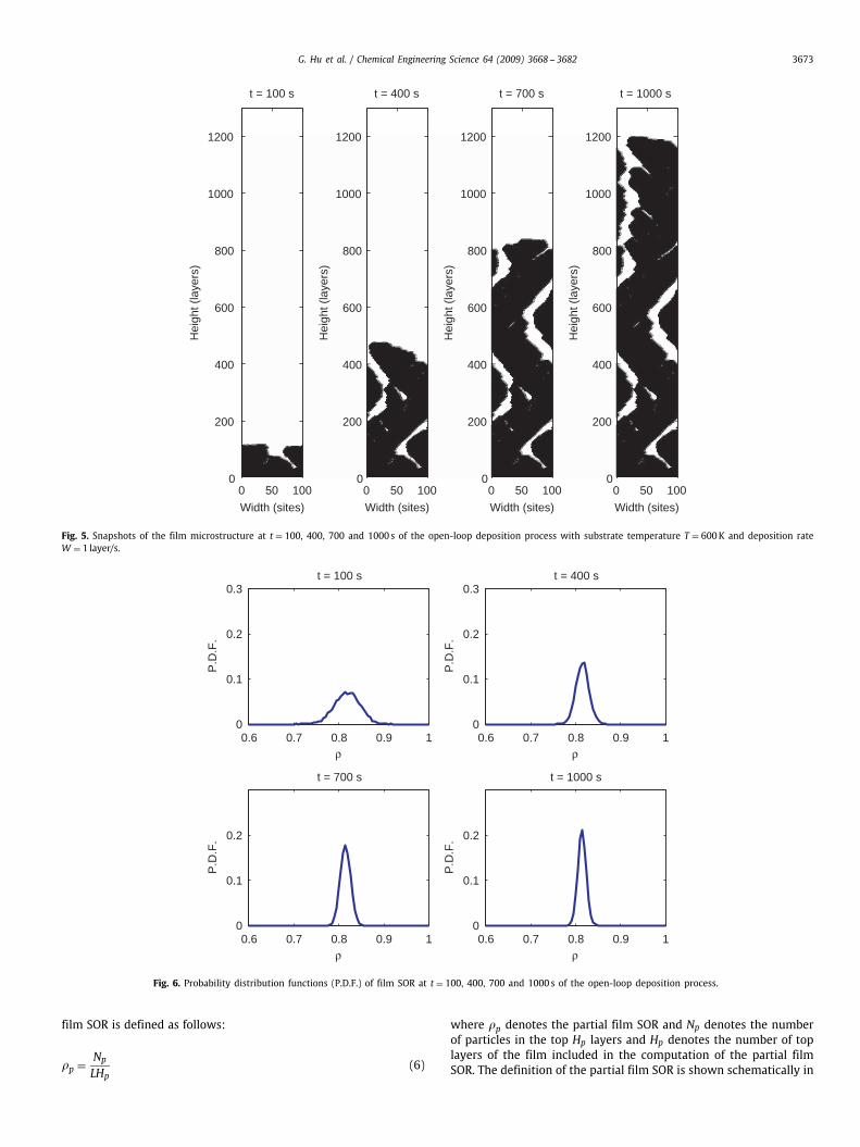
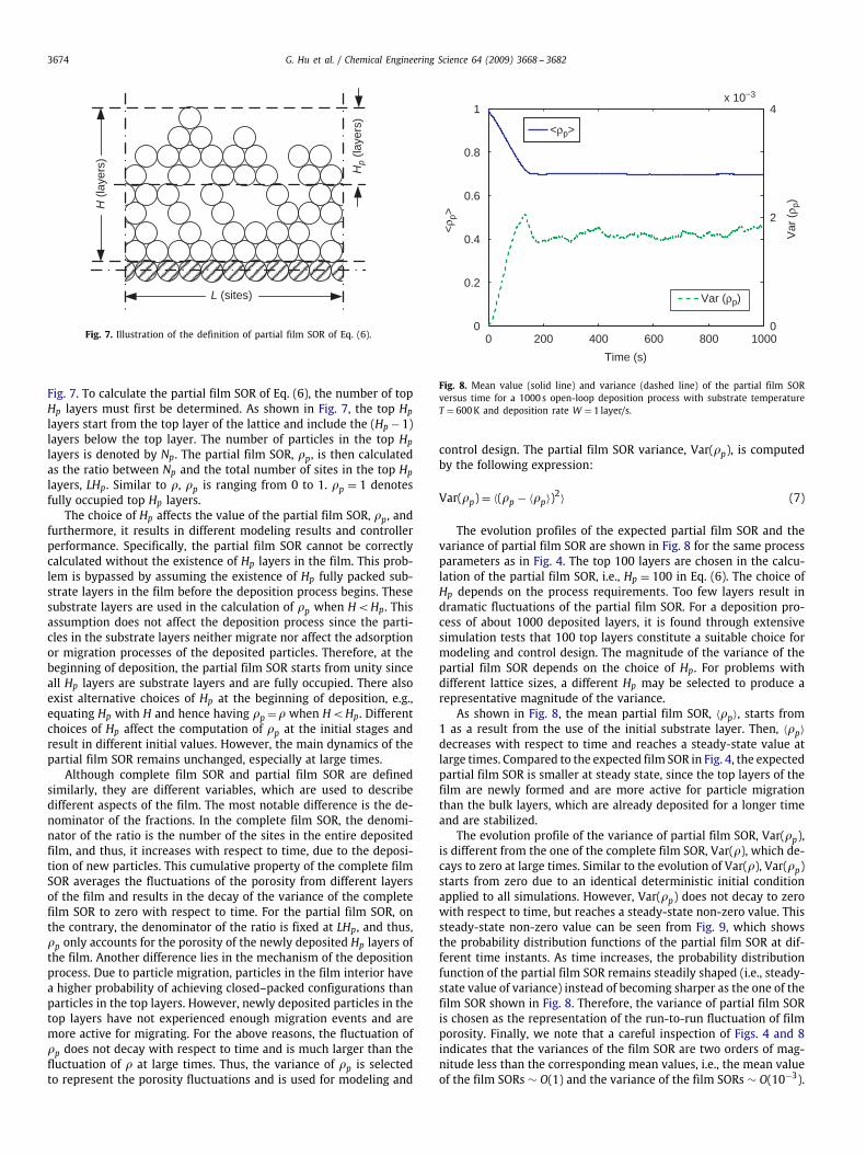
In this subsection, the thin film deposition process is simulatedaccording to the algorithm described in Section 2. The evolution offilm SOR and its variance are computed from Eqs. (4) and (5), re-spectively. The lattice size L is equal to 100 throughout this work.The choice of lattice size is determined from a balance between sta-tistical accuracy and reasonable requirements for computing power.One thousand independent simulation runs are carried out to obtainthe expected value and the variance of the film SOR. The simulationtime is 1000 s. All simulations start with an identical flat initial con-dition, i.e., only a substrate layer is present on the lattice withoutany deposited particles. Fig. 4 shows the evolution profiles of theexpected value and the variance of the film SOR during the depo-sition process for the following process parameters: T = 600K andW = 1 layer/s. In Fig. 4, the film SOR is initially 0 and as particlesbegin to deposit on the film, the film SOR increases with respect totime and quickly reaches a steady-state value. Snapshots of the thinfilm microstructure at different times, t = 100, 400, 700 and 1000 s,of the open-loop simulation are shown in Fig. 5.

0

0.2

0.4

0.6

0.8

1

Time (s)

<ρ>

0 200 400 600 800 10000

0.005

0.01

Var

(ρ)

0 50 1000

0.2

0.4

0.6

0.8

1

Time (s)

<ρ>

<ρ>

Var (ρ)

Fig. 4. Mean value (solid lines) and variance (dashed line) of the complete film SORversus time for a 1000 s open-loop deposition process with substrate temperatureT = 600K and deposition rate W = 1 layer/s.

In the snapshots of the microstructure, columnar structures areobserved, which is due to the effect of nonlocal shadowing of theexisting particles, which prevents incident particles from adsorbingto the film sites that are blocked by the particles at higher posi-tions. Such columnar structures are also observed both in the ex-periments and in simulations with similar microscopic rules (Wangand Clancy, 1998, 2001; Levine and Clancy, 2000; Zhang et al., 2004).Within the columnar structure, there exist small pores in the mi-crostructure that contribute to the film porosity. Such a structure(columns with few pores) is the result of certain deposition condi-tions, i.e., the substrate temperature and the adsorption rate consid-ered. Different conditions may result in different microstructure. Forexample, at the low-temperature region (below 500K), the depositedthin film shows a tree-like structure with a large number of smallpores.

The evolution profile of the variance starts at zero and jumps toa peak, after which the variance decays with respect to time. Thevariance is used to represent the extent of fluctuation of the filmSOR at a given time. Since all simulations start at the same initialcondition, the initial variance is zero (by convention) at time t = 0.As particles begin to deposit on the film, the variance of the filmSOR, Var(�), increases at short times and it subsequently decreasesto zero at large times. Note that the film SOR is a cumulative propertysince it accounts for all the deposited layers and particles on the film.In other words, the film SOR from each individual simulation runapproaches its expected value at large times. Thus, at large times,SOR fluctuations decrease as more layers are included into the film.It is evident from Fig. 4 that the SOR variance decays and approacheszero at large times. Fig. 6 shows the probability distribution functionsof the film SOR at different time instants. It can be clearly seen inFig. 6 that, as time increases, the probability distribution functionsbecome sharper and closer to its mean value, which shows the factthat the fluctuation of film SOR is diminishing (i.e., smaller variance)at large times. Thus, the film SOR of Eq. (4) and its variance of Eq. (5)are not suitable variables for the purposes of modeling and controlof film porosity fluctuations. Another variable must be introduced torepresent the fluctuation of the film porosity.

3.3. Partial film site occupancy ratio

In this subsection, a new concept of film SOR is introduced,termed partial film SOR, which is the film SOR calculated by account-ing only for the top Hp layers of the film. Mathematically, the partial

G. Hu et al. / Chemical Engineering Science 64 (2009) 3668 -- 3682 3673

0 50 1000

200

400

600

800

1000

1200

t = 100 s

Width (sites)

Hei

ght (

laye

rs)

0 50 1000

200

400

600

800

1000

1200

t = 400 s

Width (sites)

Hei

ght (

laye

rs)

0 50 1000

200

400

600

800

1000

1200

t = 700 s

Width (sites)

Hei

ght (

laye

rs)

0 50 1000

200

400

600

800

1000

1200

t = 1000 s

Width (sites)

Hei

ght (

laye

rs)

Fig. 5. Snapshots of the film microstructure at t = 100, 400, 700 and 1000 s of the open-loop deposition process with substrate temperature T = 600K and deposition rateW = 1 layer/s.

0.6 0.7 0.8 0.9 10

0.1

0.2

0.3t = 100 s

ρ

P.D

.F.

0.6 0.7 0.8 0.9 10

0.1

0.2

0.3t = 400 s

ρ

P.D

.F.

0.6 0.7 0.8 0.9 10

0.1

0.2

t = 700 s

ρ

P.D

.F.

0.6 0.7 0.8 0.9 10

0.1

0.2

t = 1000 s

ρ

P.D

.F.

Fig. 6. Probability distribution functions (P.D.F.) of film SOR at t = 100, 400, 700 and 1000 s of the open-loop deposition process.

film SOR is defined as follows:

�p = Np

LHp(6)

where �p denotes the partial film SOR and Np denotes the numberof particles in the top Hp layers and Hp denotes the number of toplayers of the film included in the computation of the partial filmSOR. The definition of the partial film SOR is shown schematically in

3674 G. Hu et al. / Chemical Engineering Science 64 (2009) 3668 -- 3682

L (sites)

H (l

ayer

s) Hp

(laye

rs)

Fig. 7. Illustration of the definition of partial film SOR of Eq. (6).

Fig. 7. To calculate the partial film SOR of Eq. (6), the number of topHp layers must first be determined. As shown in Fig. 7, the top Hp

layers start from the top layer of the lattice and include the (Hp − 1)layers below the top layer. The number of particles in the top Hp

layers is denoted by Np. The partial film SOR, �p, is then calculatedas the ratio between Np and the total number of sites in the top Hp

layers, LHp. Similar to �, �p is ranging from 0 to 1. �p = 1 denotesfully occupied top Hp layers.

The choice of Hp affects the value of the partial film SOR, �p, andfurthermore, it results in different modeling results and controllerperformance. Specifically, the partial film SOR cannot be correctlycalculated without the existence of Hp layers in the film. This prob-lem is bypassed by assuming the existence of Hp fully packed sub-strate layers in the film before the deposition process begins. Thesesubstrate layers are used in the calculation of �p when H<Hp. Thisassumption does not affect the deposition process since the parti-cles in the substrate layers neither migrate nor affect the adsorptionor migration processes of the deposited particles. Therefore, at thebeginning of deposition, the partial film SOR starts from unity sinceall Hp layers are substrate layers and are fully occupied. There alsoexist alternative choices of Hp at the beginning of deposition, e.g.,equating Hp with H and hence having �p =� when H<Hp. Differentchoices of Hp affect the computation of �p at the initial stages andresult in different initial values. However, the main dynamics of thepartial film SOR remains unchanged, especially at large times.

Although complete film SOR and partial film SOR are definedsimilarly, they are different variables, which are used to describedifferent aspects of the film. The most notable difference is the de-nominator of the fractions. In the complete film SOR, the denomi-nator of the ratio is the number of the sites in the entire depositedfilm, and thus, it increases with respect to time, due to the deposi-tion of new particles. This cumulative property of the complete filmSOR averages the fluctuations of the porosity from different layersof the film and results in the decay of the variance of the completefilm SOR to zero with respect to time. For the partial film SOR, onthe contrary, the denominator of the ratio is fixed at LHp, and thus,�p only accounts for the porosity of the newly deposited Hp layers ofthe film. Another difference lies in the mechanism of the depositionprocess. Due to particle migration, particles in the film interior havea higher probability of achieving closed–packed configurations thanparticles in the top layers. However, newly deposited particles in thetop layers have not experienced enough migration events and aremore active for migrating. For the above reasons, the fluctuation of�p does not decay with respect to time and is much larger than thefluctuation of � at large times. Thus, the variance of �p is selectedto represent the porosity fluctuations and is used for modeling and

10000

0.2

0.4

0.6

0.8

1

Time (s)

<ρp>

0 200 400 600 8000

2

4x 10−3

Var

(ρp)

<ρp>

Var (ρp)

Fig. 8. Mean value (solid line) and variance (dashed line) of the partial film SORversus time for a 1000 s open-loop deposition process with substrate temperatureT = 600K and deposition rate W = 1 layer/s.

control design. The partial film SOR variance, Var(�p), is computedby the following expression:

Var(�p) = 〈(�p − 〈�p〉)2〉 (7)

The evolution profiles of the expected partial film SOR and thevariance of partial film SOR are shown in Fig. 8 for the same processparameters as in Fig. 4. The top 100 layers are chosen in the calcu-lation of the partial film SOR, i.e., Hp = 100 in Eq. (6). The choice ofHp depends on the process requirements. Too few layers result indramatic fluctuations of the partial film SOR. For a deposition pro-cess of about 1000 deposited layers, it is found through extensivesimulation tests that 100 top layers constitute a suitable choice formodeling and control design. The magnitude of the variance of thepartial film SOR depends on the choice of Hp. For problems withdifferent lattice sizes, a different Hp may be selected to produce arepresentative magnitude of the variance.

As shown in Fig. 8, the mean partial film SOR, 〈�p〉, starts from1 as a result from the use of the initial substrate layer. Then, 〈�p〉decreases with respect to time and reaches a steady-state value atlarge times. Compared to the expected film SOR in Fig. 4, the expectedpartial film SOR is smaller at steady state, since the top layers of thefilm are newly formed and are more active for particle migrationthan the bulk layers, which are already deposited for a longer timeand are stabilized.

The evolution profile of the variance of partial film SOR, Var(�p),is different from the one of the complete film SOR, Var(�), which de-cays to zero at large times. Similar to the evolution of Var(�), Var(�p)starts from zero due to an identical deterministic initial conditionapplied to all simulations. However, Var(�p) does not decay to zerowith respect to time, but reaches a steady-state non-zero value. Thissteady-state non-zero value can be seen from Fig. 9, which showsthe probability distribution functions of the partial film SOR at dif-ferent time instants. As time increases, the probability distributionfunction of the partial film SOR remains steadily shaped (i.e., steady-state value of variance) instead of becoming sharper as the one of thefilm SOR shown in Fig. 8. Therefore, the variance of partial film SORis chosen as the representation of the run-to-run fluctuation of filmporosity. Finally, we note that a careful inspection of Figs. 4 and 8indicates that the variances of the film SOR are two orders of mag-nitude less than the corresponding mean values, i.e., the mean valueof the film SORs ∼ O(1) and the variance of the film SORs ∼ O(10−3).

G. Hu et al. / Chemical Engineering Science 64 (2009) 3668 -- 3682 3675

0.4 0.6 0.8 10

0.1

0.2

0.3t = 100 s

ρp

P.D

.F.

0.4 0.6 0.8 10

0.1

0.2

0.3t = 400 s

ρp

0.4 0.6 0.8 1ρp

0.4 0.6 0.8 1ρp

P.D

.F.

0

0.1

0.2

t = 700 s

P.D

.F.

0

0.1

0.2

t = 1000 s

P.D

.F.

Fig. 9. Probability distribution functions (PDF) of partial film SOR at t = 100, 400, 700 and 1000 s of the open-loop deposition process.

4. Construction of ODE models for complete and partial filmsite occupancy ratio

For control purposes, dynamic models are required that describehow the film porosity expressed in terms of complete and partial filmSOR varies with respect to potential manipulated input variables liketemperature and deposition rate. In this section, deterministic andstochastic linear ODE models are derived to describe the evolution offilm SOR. The derivation of these ODE models and the computationof their parameters is done on the basis of data obtained from thekMC model of the deposition process.

4.1. Deterministic dynamic model of complete film site occupancy ratio

From the open-loop simulation results, the dynamics of the ex-pected value of the complete film SOR evolution can be approx-imately described by a first-order ODE model. Therefore, a linearfirst-order deterministic ODE is chosen to describe the dynamics ofthe complete film SOR as follows:

�d〈�(t)〉

dt= �ss − 〈�(t)〉 (8)

where t is the time, � is the time constant and �ss is the steady-state value of the complete film SOR. The deterministic ODE systemof Eq. (10) is subject to the following initial condition:

〈�(t0)〉 = �0 (9)

where t0 is the initial time and �0 is the initial value of the completefilm SOR. Note that �0 is a deterministic variable, since �0 refers tothe expected value of the complete film SOR at t = t0. From Eqs. (8)and (9), it follows that

〈�(t)〉 = �ss + (�0 − �ss)e−(t−t0)/� (10)

The model parameters, � and �ss, depend on substrate tem-perature. This dependence will be mathematically expressed inSection 4.3.

4.2. Stochastic dynamic model of partial film site occupancy ratio

To regulate the variance of the partial film SOR, a stochastic modelmust be used. For simplicity, a linear stochastic ODE is used to modelthe dynamics of the partial film SOR. Similar to the deterministicODE model for the expected complete film SOR of Eq. (8), a first-order stochastic ODE is chosen for the computation of the partialfilm SOR as follows:

�pd�p(t)

dt= �ss

p − �p(t) + p(t) (11)

where �ssp and �p are the two model parameters which denote the

steady-state value of the partial film SOR and the time constant,respectively, and p(t) is a Gaussian white noise with the followingexpressions for its mean and covariance:

〈p(t)〉 = 0

〈p(t)p(t′)〉 = 2

p�(t − t′) (12)

where p is a parameter which measures the intensity of theGaussian white noise and �(·) denotes the standard Dirac deltafunction. The model parameters �ss

p , �p and p are functions of thesubstrate temperature. We note that p(t) is taken to be a Gaussianwhite noise because the values of �p obtained from 10, 000 inde-pendent kMC simulations of the deposition process at large timesare in closed accord with a Gaussian distribution law: see Fig. 10for the histogram of the partial film SOR at t = 1000 s.

The stochastic ODE system of Eq. (11) is subject to the followinginitial condition:

�p(t0) = �p0 (13)

3676 G. Hu et al. / Chemical Engineering Science 64 (2009) 3668 -- 3682

0.5 0.55 0.6 0.65 0.7 0.75 0.8 0.85 0.90

500

1000

1500

ρp

Cou

nts

Fig. 10. Histogram from 10, 000 simulation runs of the partial film SOR at the end(t=1000 s) of the open-loop deposition process with substrate temperature T=600Kand deposition rate W = 1 layer/s.

where �p0 is the initial value of the partial film SOR. Note that �p0is a random number, which follows a Gaussian distribution.

The following analytical solution to Eq. (11) can be obtained froma direct computation as follows:

�p(t) = �ssp + (�p0 − �ss

p )e−(t−t0)/�p +

∫ t

t0e−(s−t0)/�pp ds. (14)

In Eq. (14), �p(t) is a random process, the expected value of which,〈�p(t)〉, can be obtained as follows:

〈�p(t)〉 = �ssp + (〈�p0〉 − �ss

p )e−(t−t0)/�p . (15)

The analytical solution of Var(�p) can be obtained from the solu-tion to Eq. (14) using the following result (Åstrom, 1970):

Result 1. If (1) f (x) is a deterministic function, (2) �(x) is a randomprocess with 〈�(x)〉 = 0 and covariance 〈�(x)�(x′)〉 = 2�(x − x′), and(3) �=∫ b

a f (x)�(x)dx, then � is a real random variable with 〈�〉=0 and

variance 〈�2〉 = 2 ∫ ba f 2(x)dx.

Using Result 1, the variance of the partial film SOR, Var(�p), canbe obtained from the analytical solution to Eq. (14) as follows:

Var(�p(t)) = �p2p

2+(Var(�p0) − �p2

p

2

)e−2(t−t0)/�p (16)

where Var(�p0) is the variance of the partial film SOR at time t = 0,which is calculated as follows:

Var(�p0) = 〈(�p0 − 〈�p0〉)2〉 (17)

A new model parameter, Varssp , is introduced to simplify the so-lution of Var(�p) in Eq. (16) as follows:

Varssp = �p2p

2(18)

where Varssp stands for the steady-state value of the variance of thepartial film SOR. With the introduction of this newmodel parameter,

the solution of the variance of the partial film SOR, Var(�p), can berewritten in the following form:

Var(�p(t)) = Varssp + (Var(�p0) − Varssp )e−2(t−t0)/�p (19)

4.3. Parameter estimation and dependence on the process parameters

Referring to the deterministic and stochastic ODE models ofEqs. (8) and (11), we note that they include five parameters, �ss, �,�ssp , �s and Varssp . The five parameters describe the dynamics of the

film SOR accounting for the effect of fluctuations. These parametersmust be estimated by comparing the predicted evolution profilesfrom the ODE models and the ones from the kMC simulation of thedeposition process. Least-square methods are used to estimate themodel parameters so that the ODE model predictions are close in aleast-square sense to the kMC simulation data.

4.3.1. Parameter estimationSince the ODE models of Eqs. (8) and (11) are linear, the five pa-

rameters, �ss, �, �ssp , �p and Varssp , can be estimated from the solu-

tions to Eqs. (10) and (15). Specifically, the parameters �ssp and �p are

estimated using Eq. (10) and the parameters �ssp , �p and Varssp are es-

timated using Eq. (15), solving two separate least-square problems.Specifically, the two least-square problems can be solved indepen-dently to obtain the first four model parameters. The steady-statevariance, Varssp , is obtained from the values of the variance evolutionprofiles at large times.

The parameters �ss and � are estimated by minimizing the sum ofthe squared difference between the evolution profiles from the ODEmodel prediction and the kMC simulation at different time instantsas follows:

min�ss ,�

m∑i=1

[〈�(ti)〉 − (�ss + (�0 − �ss)e−(t−t0)/�)]2 (20)

where m is the number of the data pairs, (ti, 〈�(ti)〉), from the kMCsimulations. Similarly, �ss

p and �p can be obtained by solving thefollowing least-square optimization problem expressed in terms ofthe expected partial film SOR:

min�ssp ,�p

m∑i=1

[〈�p(ti)〉 − (�ssp + (�p0 − �ss

p )e−(t−t0)/�p )]2 (21)

The data used for the parameter estimation are obtained fromthe open-loop kMC simulation of the thin film growth process. Theprocess parameters are fixed during each open-loop simulation sothat the dependence of the model parameters on the process param-eters can be obtained for fixed operation conditions. The completefilm SOR and the partial film SOR are calculated on the basis of thedeposited film at specific time instants. Due to the stochastic natureof the process, multiple independent simulation runs are performedto obtain the expected values of the complete film SOR and of thepartial film SOR as well as of the variance of the partial film SOR.

The above parameter estimation process is applied to the open-loop simulation results. First, the open-loop evolution profiles of thecomplete film SOR and of the partial film SOR are obtained from1000 independent kMC simulation runs with substrate temperatureT = 600K and deposition rate W = 1 layer/s. Subsequently, the de-terministic and stochastic ODE models of Eqs. (8) and (11) are com-paredwith the open-loop kMC simulation data to compute themodelparameters using least-square methods. Figs. 11 and 12 show theopen-loop profiles and the predicted profiles of 〈�〉, 〈�p〉 and Var(�p)from the ODE models with the estimated parameters as follows:

�ss = 0.8178, � = 1.6564 s

�ssp = 0.6957, �p = 77.2702 s, Varssp = 1.6937 × 10−3 (22)

G. Hu et al. / Chemical Engineering Science 64 (2009) 3668 -- 3682 3677

0

0.1

0.2

0.3

0.4

0.5

0.6

0.7

0.8

0.9

1

Time (s)

<ρ>

0 200 400 600 800 10000

0.1

0.2

0.3

0.4

0.5

0.6

0.7

0.8

0.9

1

<ρp>

<ρ>: kMC output<ρ>: prediction

<ρp>: kMC output

<ρp>: prediction

Fig. 11. Profiles of the expected value of the complete film SOR (solid line) andof the partial film SOR (dashed line) with respect to time for a 1000 s open-loopdeposition process and predictions from the deterministic ODE model (solid linewith `+') and the stochastic ODE model (dashed line with `+') with estimatedparameters; T = 600K, W = 1 layer/s.

0 200 400 600 800 10000

0.5

1

1.5

2

2.5x 10−3

Time (s)

Var

(ρp)

Fig. 12. Variance of the partial film SOR with respect to time for a 1000 s open-loopdeposition process (solid line) and the estimated steady-state level (dashed line);T = 600K, W = 1 layer/s.

The predictions from the ODE models are very close to the open-loop kMC simulation profiles, which indicates that the dynamics ofthe film SOR can be adequately described by first-order ODEs. Thereis, however, some mismatch of the predicted ODE-based profilesfrom the kMC data, especially for the expected value of the completefilm SOR. This is because the dynamics of the complete film SORdepend on the total height of the film. A film at initial stages is verythin and the complete film SOR changes significantly as more layersare deposited, while a film at large times is much thicker and thecomplete film SOR is relatively insensitive to the newly depositedlayers. Since a first-order ODE model is used to capture the dynamicsof the complete film SOR, the time constant, �, is chosen to strikea balance between the initial and final stages of the film growth.Therefore, the predictions from the ODE model cannot match theopen-loop profiles, obtained from the kMC models, perfectly at alltimes. Overall, the computed first-order ODE models approximate

300 400 500 600 700 8000.2

0.3

0.4

0.5

0.6

0.7

0.8

0.9

1

Substrate temperature T (K)

ρss,ρ

ss

ρss

ρssp

p

Fig. 13. Dependence of �ss and �ssp on the substrate temperature with deposition

rate W = 1 layer/s.

well the dynamics of the film SOR and its fluctuation, and thus, theycan be used for the purpose of feedback control design. The closed-loop system simulation results using these first-order models willbe discussed in Section 5.3.

The lattice size dependence of the steady-state value of the com-plete film SOR is shown in Fig. 16. It can be clearly seen that the filmSOR depends on the lattice size. To achieve near lattice-size indepen-dence, a very large lattice size is required and cannot be simulatedusing the available amount of computing power. The purpose of theproposed modeling method is to identify the film SOR models fromthe output of the given deposition process, which can be from eithera kMC simulator or experimental deposition process data. Note thatthe applicability of the proposed modeling method is not limited toany specific lattice size. In this work, a model with lattice size of100 captures the film SOR dynamics and allows obtaining sufficientstatistical accuracy in terms of computing the expected values andvariances of film SORs.

4.3.2. Dependence of model parameters on process parametersThe model parameters of the ODE models of Eqs. (8) and (11) de-

pend on two process parameters, temperature and deposition rate.This dependence is used in the formulation of the model predictivecontrol design in the next section when solving the optimizationproblem. Thus, parameter estimation from open-loop kMC simula-tion results of the thin film growth process for a variety of process pa-rameters is performed to obtain the relationship between the modelparameters and the process parameters. In this work, the depositionrate for all simulations is fixed at 1 layer/s and the only manipu-lated input considered is the substrate temperature, T. The range ofT is between 300 and 800K, which is from room temperature to theupper limit of the allowable temperature for a valid on-lattice kMCmodel of silicon film. The dependence of the model parameters onthe substrate temperature is shown in Figs. 13–15. In these figures, itcan be clearly seen that the dependence of the model parameters ontemperature is highly nonlinear. For most model parameters, thereare asymptotes at the low temperature region due to the limitedsurface migration rates at low temperatures. However, at high tem-peratures, �ss and �ss

p approach unity, which corresponds to a fullypacked film, i.e., all film sites are occupied by particles.

3678 G. Hu et al. / Chemical Engineering Science 64 (2009) 3668 -- 3682

1

1.5

2

2.5

3

Substrate temperature T (K)

τ

300 400 500 600 700 8000

200

400

600

800

τ p

τ

τp

Fig. 14. Dependence of � and �p on the substrate temperature with deposition rateW = 1 layer/s.

300 400 500 600 700 8000

0.2

0.4

0.6

0.8

1

1.2

1.4

1.6

1.8x 10−3

Substrate temperature T (K)

Varss p

Fig. 15. Dependence of Varssp on the substrate temperature with deposition rateW = 1 layer/s.

5. Model predictive control design

In this section, we design model predictive controllers based onthe deterministic and stochastic ODE models of Eqs. (8) and (11)to simultaneously control the complete film SOR of the depositionprocess to a desired level and minimize the variance of the partialfilm SOR. State feedback controllers are considered in this work, i.e.,the values of the complete film SOR and of the partial film SOR areassumed to be available for feedback control. Real-time film SORcan be estimated from in situ thin film thickness measurements(Buzea and Robbie, 2005) in combination with off-line film porositymeasurements.

5.1. Regulation of complete film site occupancy ratio

Since the film porosity is the main control objective in this work,we first consider the problem of regulation of the expected com-plete film SOR to a desired level, �set , within a model predictivecontrol framework. The substrate temperature is used as the ma-

102 103 104 1050

0.1

0.2

0.3

0.4

0.5

0.6

0.7

0.8

0.9

1

Lattice size, L

ρss

T = 400T = 500

Fig. 16. Dependence of steady-state values of film SOR, �ss , on the lattice size fordifferent temperatures.

nipulated input and the deposition rate is fixed at a certain value,W0, during the entire closed-loop simulation. To account for a num-ber of practical considerations, several constraints are added to thecontrol problem. First, there is a constraint on the range of varia-tion of the substrate temperature. This constraint ensures validityof the on-lattice kMC model. Another constraint is imposed on therate of change of the substrate temperature to account for actuatorlimitations.

We note that classical control schemes like proportional-integral(PI) control cannot be designed to explicitly account for input/stateconstraints, optimality considerations and the batch nature of thedeposition process, and thus, their use will not be pursued in thiswork. Furthermore, dynamic open-loop optimization may be usedbut it does not provide robustness against the model inaccuraciesand the fluctuations in the deposition process. In the case wherefeedback porosity control cannot be attained, dynamic optimizationmay be used instead; this is naturally included in the proposedmodelpredictive control framework.

The control action, at a time t and state �, is obtained by solv-ing a finite-horizon optimal control problem. The optimal tempera-ture profile is calculated by solving a finite-dimensional optimizationproblem in a receding horizon fashion. Specifically, the MPC problemis formulated based on the deterministic ODE of Eq. (8) as follows:

minT1,. . .,Ti ,. . .,Tp

J(�(t)) =p∑

i=1

qsp,i[�set − 〈�(t + i )〉]2

s.t. 〈�(t + i )〉 = �ss(Ti,W0) + (〈�(t + (i − 1) )〉− �ss(Ti,W0))e− /�(Ti ,W0)

Tmin <Ti <Tmax∣∣∣∣Ti+1 − Ti

∣∣∣∣ �LT

i = 1, 2, . . . , p (23)

where t is the current time, is the sampling time, p is the numberof prediction steps, p is the specified prediction horizon, Ti, i =1, 2, . . . , p, is the substrate temperature at the ith step (Ti = T(t+ i )),respectively,W0 is the fixed deposition rate, qsp,i, i=1, 2, . . . , p, are theweighting penalty factors for the error of the complete film SOR atthe ith prediction step, Tmin and Tmax are the lower and upper boundson the substrate temperature, respectively, and LT is the limit on therate of change of the substrate temperature. In the MPC formulationof Eq. (23), J is the cost function, which contains penalty on the

G. Hu et al. / Chemical Engineering Science 64 (2009) 3668 -- 3682 3679

squared difference between the desired value of the complete filmSOR, �set , and the predicted values of this variable at all time steps.

The dynamics of the expected value of the complete film SOR aredescribed by the deterministic first-order ODE of Eq. (10). The de-pendence of model parameters on process parameters is obtainedfrom the parameter estimation at a variety of conditions. Due tothe availability of analytical solutions of the linear ODE model ofEq. (10), these analytical solutions can be used directly in the MPCformulation of Eq. (23) for the prediction of 〈�(t)〉. The system state,�(t), is the complete film SOR at time t. Note that �(t), which isobtained directly from the simulation in real-time, is considered asthe expected complete film SOR and can be used as an initial con-dition for the solution of the deterministic ODE of Eq. (10). In theclosed-loop simulations, the instantaneous values of � and �p aremade available to the controller at each sampling time; however, nostatistical information, e.g., the expected value of complete/partialfilm SOR, is available for feedback. The optimal set of control actions,(T1, T2, . . . , Tp), is obtained from the solution of the multi-variable op-timization problem of Eq. (23), and only the first value of the ma-nipulated input trajectory, T1, is applied to the deposition processduring the time interval (t, t+ ). At time t+ , a new measurementof � is received and the MPC problem of Eq. (23) is solved for thenext control input trajectory.

5.2. Fluctuation regulation of partial film site occupancy ratio

Reduction of run-to-run variability is another goal in process con-trol of a thin film growth process. In this work, the fluctuation offilm SOR is represented by the variance of partial film SOR, Var(�p).Ideally, a zero value means no fluctuation from run to run. However,it is impossible to achieve zero variance of partial film SOR due tothe stochastic nature of the thin film growth process. Thus, the con-trol objective of fluctuation regulation is to minimize the varianceby manipulating the process parameters.

In this work, the fluctuation is included into the cost functiontogether with the error of the complete film SOR. Specifically, theMPC formulation with penalty on the error of the expected completefilm SOR and penalty on the variance of the partial film SOR is givenas follows:

minT1,. . .,Ti ,. . .,Tp

J(�(t)) =p∑

i=1

{qsp,i[�set − 〈�(t + i )〉]2 (24)

+ qvar,iVar[�p(t + i )]}s.t. 〈�(t + i )〉 = �ss(Ti,W0) + (〈�(t + (i − 1) )〉

− �ss(Ti,W0))e− /�(Ti ,W0)

Var(�p(t + i )) = Varssp (Ti,W0) + (Var[�p(t + (i − 1) )]

− Varssp (Ti,W0))e−2 /�p(Ti ,W0)

Tmin <Ti <Tmax∣∣∣∣Ti+1 − Ti

∣∣∣∣ �LT

i = 1, 2, . . . , p (25)

where qsp,i and qvar,i, i = 1, 2, . . . , p, are weighting penalty factors onthe error of the complete film SOR and of the variance of the partialfilm SOR, respectively. Other variables in Eq. (24) are defined similarto the ones in Eq. (23). The same constraints as in Eq. (23) are im-posed on the MPC formulation of Eq. (24). Due to the unavailabilityof statistical information of the partial film SOR in real-time, the ini-tial condition of the partial film SOR is regarded as a deterministicvariable and the initial condition for Var(�p(t)) is considered to bezero in the MPC formulation.

0

0.1

0.2

0.3

0.4

0.5

0.6

0.7

0.8

0.9

1

Time (s)

ρ, <

ρ>

0 200 400 600 800 1000300

350

400

450

500

550

600

650

700

750

800

T (K

)

<ρ>ρset−point

substrate temperature

Fig. 17. Closed-loop profiles of the complete film SOR (solid line) and of the expectedvalue of the complete film SOR (dotted line) under the controller of Eq. (23). Theprofile of the substrate temperature is also included (dash-dotted line).

5.3. Closed-loop simulations

In this section, the model predictive controllers of Eqs. (23) and(24) are applied to the kMC model of the thin film growth processdescribed in Section 2. The value of the substrate temperature is ob-tained from the solution to the problem of Eqs. (23) and (24) at eachsampling time and is applied to the closed-loop system until thenext sampling time. The complete film SOR and the partial film SORare obtained directly from the kMC model of the thin film at eachsampling time as the state of the system and are fed into the con-trollers. The sampling time is fixed in all closed-loop simulations tobe =5 s, which is in the same order of magnitude of the time con-stant of the dynamics of the complete film SOR, �. The optimizationproblems in the MPC formulations of Eqs. (23) and (24) are solvedusing a local constrained minimization algorithm.

The constraint on the rate of change of the substrate temperatureis imposed onto the optimization problem, which is realized in theoptimization process in the following way:

∣∣∣∣Ti+1 − Ti

∣∣∣∣ �LT ⇒ |Ti+1 − Ti|�LT ⇒ Ti − LT �Ti+1�Ti + LT ,

i = 1, 2, . . . , p. (26)

The desired value (set-point) for the complete film SOR in the closed-loop simulations is 0.9. The number of prediction steps is 5. Thedeposition rate is fixed at 1 layer/s and all closed-loop simulationsare initialized with an initial temperature of 300K. The maximal rateof change of the temperature is 10K/s. Expected values and variancesare calculated from 1000 independent simulation runs.

5.3.1. Regulation of complete film site occupancy ratioFirst, the closed-loop simulation results of complete film SOR reg-

ulation using the model predictive control formulation of Eq. (23) areprovided. In this MPC formulation, the cost function contains onlypenalty on the difference of the complete film SOR from the set-pointvalue. Specifically, the optimization problem is formulated to min-imize the difference between the complete film SOR set-point andthe prediction of the expected complete film SOR at the end of eachprediction step. All weighting penalty factors, qsp,i, i = 1, 2, . . . , p, areassigned to be equal. Fig. 17 shows the profiles of the expected valueof the complete film SOR in the closed-loop system simulation. Theprofiles of the complete film SOR and of the substrate temperaturefrom a single simulation run are also included in Fig. 17.

3680 G. Hu et al. / Chemical Engineering Science 64 (2009) 3668 -- 3682

0 50 1000

200

400

600

800

1000

1200

t = 100 s

Width (sites)

Hei

ght (

laye

rs)

0 50 1000

200

400

600

800

1000

1200

t = 400 s

Width (sites)

Hei

ght (

laye

rs)

0 50 1000

200

400

600

800

1000

1200

t = 700 s

Width (sites)

Hei

ght (

laye

rs)

0 50 1000

200

400

600

800

1000

1200

t = 1000 s

Width (sites)

Hei

ght (

laye

rs)

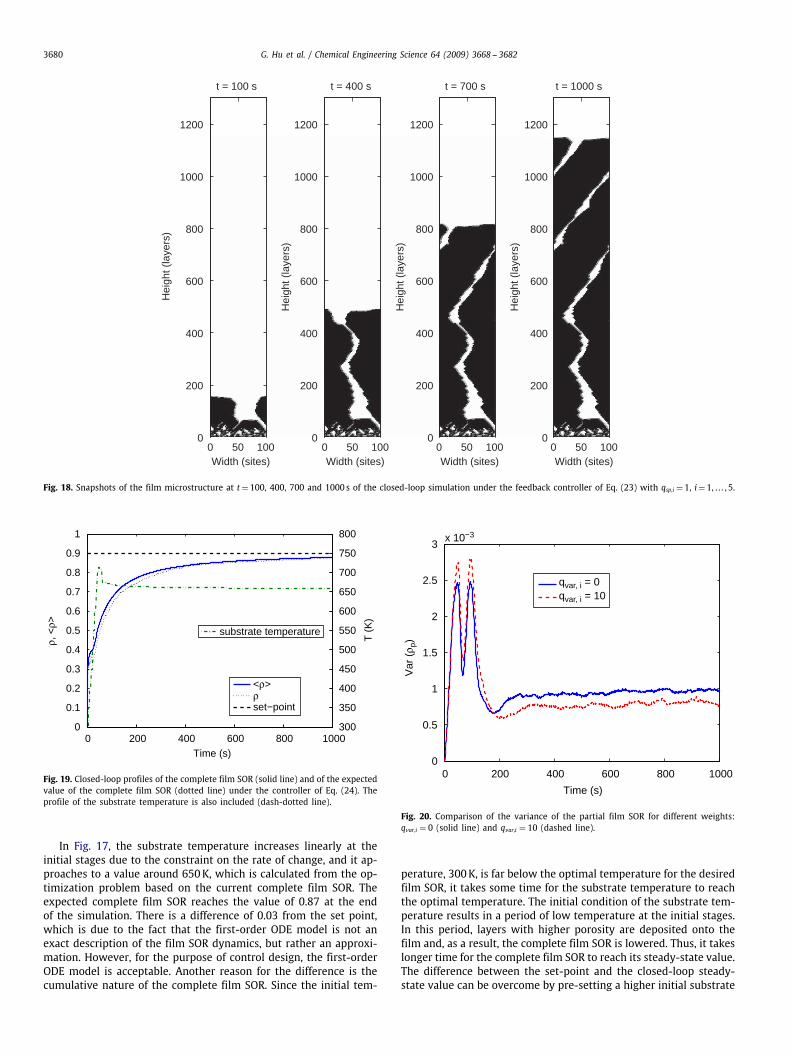
Fig. 18. Snapshots of the film microstructure at t= 100, 400, 700 and 1000 s of the closed-loop simulation under the feedback controller of Eq. (23) with qsp,i = 1, i= 1, . . . , 5.

0

0.1

0.2

0.3

0.4

0.5

0.6

0.7

0.8

0.9

1

Time (s)

ρ, <

ρ>

0 200 400 600 800 1000300

350

400

450

500

550

600

650

700

750

800

T (K

)

<ρ>ρset−point

substrate temperature

Fig. 19. Closed-loop profiles of the complete film SOR (solid line) and of the expectedvalue of the complete film SOR (dotted line) under the controller of Eq. (24). Theprofile of the substrate temperature is also included (dash-dotted line).

In Fig. 17, the substrate temperature increases linearly at theinitial stages due to the constraint on the rate of change, and it ap-proaches to a value around 650K, which is calculated from the op-timization problem based on the current complete film SOR. Theexpected complete film SOR reaches the value of 0.87 at the endof the simulation. There is a difference of 0.03 from the set point,which is due to the fact that the first-order ODE model is not anexact description of the film SOR dynamics, but rather an approxi-mation. However, for the purpose of control design, the first-orderODE model is acceptable. Another reason for the difference is thecumulative nature of the complete film SOR. Since the initial tem-

0 200 400 600 800 10000

0.5

1

1.5

2

2.5

3 x 10−3

Time (s)

Var

(ρp)

qvar, i = 0qvar, i = 10

Fig. 20. Comparison of the variance of the partial film SOR for different weights:qvar,i = 0 (solid line) and qvar,i = 10 (dashed line).

perature, 300K, is far below the optimal temperature for the desiredfilm SOR, it takes some time for the substrate temperature to reachthe optimal temperature. The initial condition of the substrate tem-perature results in a period of low temperature at the initial stages.In this period, layers with higher porosity are deposited onto thefilm and, as a result, the complete film SOR is lowered. Thus, it takeslonger time for the complete film SOR to reach its steady-state value.The difference between the set-point and the closed-loop steady-state value can be overcome by pre-setting a higher initial substrate

G. Hu et al. / Chemical Engineering Science 64 (2009) 3668 -- 3682 3681

0 50 1000

200

400

600

800

1000

1200

t = 100 s

Width (sites)

Hei

ght (

laye

rs)

0 50 1000

200

400

600

800

1000

1200

t = 400 s

Width (sites)

Hei

ght (

laye

rs)

0 50 1000

200

400

600

800

1000

1200

t = 700 s

Width (sites)

Hei

ght (

laye

rs)

0 50 1000

200

400

600

800

1000

1200

t = 1000 s

Width (sites)

Hei

ght (

laye

rs)

Fig. 21. Snapshots of the film microstructure at t = 100, 400, 700 and 1000 s of the closed-loop simulation under the feedback controller of Eq. (24) with qsp,i = 1, qvar,i = 10,i = 1, . . . , 5.

temperature. Another possible method to improve the closed-loopperformance is to replace the quadratic cost function that penalizesthe deviation of the SORs from the desired values with other func-tions, since quadratic terms slow down the convergence speed inthe vicinity of the set point. Snapshots of the film microstructureat different times, t = 100, 400, 700 and 1000 s, of the closed-loopsimulation are shown in Fig. 18.

5.3.2. Fluctuation regulation of partial film site occupancy ratioTo reduce the run-to-run variability of the film porosity, the vari-

ance of the partial film SOR is added into the cost function in themodel predictive controller of Eq. (24). There are two weighting fac-tors, qsp,i and qvar,i, which represent the weights on the completefilm SOR and on the variance of the partial film SOR prediction, re-spectively. Fig. 19 shows the profiles of the expected complete filmSOR and of the substrate temperature in the closed-loop simulation,with the following values assigned to the weighting factors:

qsp,i = 1, qvar,i = 10, i = 1–5. (27)

As shown in Fig. 19, the complete film SOR and the substratetemperature evolve similarly as in Fig. 17. However, with the costfunction including penalty on the variance of the partial film SOR,the optimal temperature is higher than the one in Fig. 17, since ahigher substrate temperature is in favor of decreasing run-to-runfluctuations. Fig. 20 shows a comparison of the variance of the partialfilm SOR between the two model predictive controllers with qvar,i =0 and qvar,i = 10, i = 1–5. It can be seen that the variance of thepartial film SOR is lowered with penalty on this variable includedinto the cost function of the MPC formulation. Snapshots of the filmmicrostructure at different times, t=100, 400, 700 and 1000 s, of theclosed-loop simulation are shown in Fig. 21.

6. Conclusions

In this work, systematic methodologies were developed for mod-eling and control of film porosity in thin film deposition. A thin filmdeposition process which involves atom adsorption and migrationwas introduced and was modeled using a triangular lattice-basedkMC simulator which allows porosity, vacancies and overhangs todevelop and leads to the deposition of a porous film. Appropriatedefinitions of film SOR and its fluctuation were introduced to de-scribe film porosity. Deterministic and stochastic ODE models werederived that describe the time evolution of film SOR and its fluctua-tion. The coefficients of the ODE models were estimated on the basisof data obtained from the kMC simulator of the deposition processusing least-square methods and their dependence on substrate tem-perature was determined. The developed ODE models were used asthe basis for the design of MPC algorithms that include penalty onthe film SOR and its variance to regulate the expected value of filmSOR at a desired level and reduce run-to-run fluctuations. The ap-plicability and effectiveness of the proposed modeling and controlmethods were demonstrated by simulation results in the context ofthe deposition process under consideration.

Acknowledgment

Financial support fromNSF, CBET-0652131, is gratefully acknowl-edged.

References

Åstrom, K.J., 1970. Introduction to Stochastic Control Theory. Academic Press,New York.

Armaou, A., Siettos, C.I., Kevrekidis, I.G., 2004. Time-steppers and `coarse' control ofdistributed microscopic processes. International Journal of Robust and NonlinearControl 14, 89–111.

3682 G. Hu et al. / Chemical Engineering Science 64 (2009) 3668 -- 3682

Ballestad, A., Ruck, B.J., Schmid, J.H., Adamcyk, M., Nodwell, E., Nicoll, C., Tiedje,T., 2002. Surface morphology of GaAs during molecular beam epitaxy growth:comparison of experimental data with simulations based on continuum growthequations. Physical Review B 65, 205302.

Bohlin, T., Graebe, S.F., 1995. Issues in nonlinear stochastic grey-boxidentification. International Journal of Adaptive Control and Signal Processing 9,465–490.

Buzea, C., Robbie, K., 2005. State of the art in thin film thickness and depositionrate monitoring sensors. Reports on Progress in Physics 68, 385–409.

Christofides, P.D., Armaou, A., Lou, Y., Varshney, A., 2008. Control and Optimizationof Multiscale Process Systems. Birkhauser, Boston.

Cuerno, R., Makse, H.A., Tomassone, S., Harrington, S.T., Stanley, H.E., 1995. Stochasticmodel for surface erosion via ion sputtering: Dynamical evolution from ripplemorphology to rough morphology. Physical Review Letters 75, 4464–4467.

Edwards, S.F., Wilkinson, D.R., 1982. The surface statistics of a granular aggregate.Proceedings of the Royal Society of London Series A—Mathematical Physical andEngineering Sciences 381, 17–31.

Fichthorn, K.A., Weinberg, W.H., 1991. Theoretical foundations of dynamical MonteCarlo simulations. Journal of Chemical Physics 95, 1090–1096.

Gillespie, D.T., 1976. A general method for numerically simulating the stochastictime evolution of coupled chemical reactions. Journal of Computational Physics22, 403–434.

Hu, G., Lou, Y., Christofides, P.D., 2008a. Dynamic output feedback covariance controlof stochastic dissipative partial differential equations. Chemical EngineeringScience 63, 4531–4542.

Hu, G., Lou, Y., Christofides, P.D., 2008b. Model parameter estimation and feedbackcontrol of surface roughness in a sputtering process. Chemical EngineeringScience 63, 1800–1816.

Kan, H.C., Shah, S., Tadyyon-Eslami, T., Phaneuf, R.J., 2004. Transient evolutionof surface roughness on patterned GaAs(001) during homoepitaxial growth.Physical Review Letters 92, 146101.

Kardar, M., Parisi, G., Zhang, Y.C., 1986. Dynamic scaling of growing interfaces.Physical Review Letters 56, 889–892.

Keršulis, S., Mitin, V., 1995. Monte Carlo simulation of growth and recovery ofsilicon. Material Science & Engineering B 29, 34–37.

Kloster, G., Scherban, T., Xu, G., Blaine, J., Sun, B., Zhou, Y., 2002. Porosity effects onlow-k dielectric film strength and interfacial adhesion. In: Proceedings of theIEEE 2002 International Interconnect Technology Conference.pp. 242–244.

Kristensen, N.R., Madsen, H., Jorgensen, S.B., 2004. Parameter estimation in stochasticgrey-box models. Automatica 40, 225–237.

Lauritsen, K.B., Cuerno, R., Makse, H.A., 1996. Noisy Kuramote–Sivashinsky equationfor an erosion model. Physical Review E 54, 3577–3580.

Levine, S.W., Clancy, P., 2000. A simple model for the growth of polycrystalline Siusing the kinetic Monte Carlo simulation. Modelling and Simulation in MaterialsScience and Engineering 8, 751–762.

Lou, Y., Christofides, P.D., 2003a. Estimation and control of surface roughness in thinfilm growth using kinetic Monte-Carlo models. Chemical Engineering Science58, 3115–3129.

Lou, Y., Christofides, P.D., 2003b. Feedback control of growth rate and surfaceroughness in thin film growth. A.I.Ch.E. Journal 49, 2099–2113.

Lou, Y., Christofides, P.D., 2004. Feedback control of surface roughness of GaAs (001)thin films using kinetic Monte-Carlo models. Computers & Chemical Engineering29, 225–241.

Lou, Y., Christofides, P.D., 2005a. Feedback control of surface roughness in sputteringprocesses using the stochastic Kuramoto–Sivashinsky equation. Computers &Chemical Engineering 29, 741–759.

Lou, Y., Christofides, P.D., 2005b. Feedback control of surface roughness usingstochastic PDEs. A.I.Ch.E. Journal 51, 345–352.

Lou, Y., Christofides, P.D., 2006. Nonlinear feedback control of surface roughnessusing a stochastic PDE: design and application to a sputtering process. Industrial& Engineering Chemistry Research 45, 7177–7189.

Lou, Y., Hu, G., Christofides, P.D., 2008. Model predictive control of nonlinearstochastic partial differential equations with application to a sputtering process.A.I.Ch.E. Journal 54, 2065–2081.

Makov, G., Payne, M.C., 1995. Periodic boundary conditions in ab initio calculations.Physical Review B 51, 4014–4022.

Maksym, P.B., 1988. Fast Monte Carlo simulation of MBE growth. SemiconductorScience and Technology 3, 594–596.

Ni, D., Christofides, P.D., 2005a. Dynamics and control of thin film surfacemicrostructure in a complex deposition process. Chemical Engineering Science60, 1603–1617.

Ni, D., Christofides, P.D., 2005b. Multivariable predictive control of thin filmdeposition using a stochastic PDE model. Industrial & Engineering ChemistryResearch 44, 2416–2427.

Reese, J.S., Raimondeau, S., Vlachos, D.G., 2001. Monte Carlo algorithms for complexsurface reaction mechanisms: efficiency and accuracy. Journal of ComputationalPhysics 173, 302–321.

Shitara, T., Vvedensky, D.D., Wilby, M.R., Zhang, J., Neave, J.H., Joyce, B.A., 1992.Step-density variations and reflection high-energy electron-diffraction intensityoscillations during epitaxial growth on vicinal GaAs(001). Physical Review B 46,6815–6824.

Siettos, C.I., Armaou, A., Makeev, A.G., Kevrekidis, I.G., 2003. Microscopic/stochastictimesteppers and “coarse” control: a kMC example. A.I.Ch.E. Journal 49,1922–1926.

Varshney, A., Armaou, A., 2005. Multiscale optimization using hybrid PDE/kMCprocess systems with application to thin film growth. Chemical EngineeringScience 60, 6780–6794.

Varshney, A., Armaou, A., 2006. Identification of macroscopic variables for low-ordermodeling of thin-film growth. Industrial & Engineering Chemistry Research 45,8290–8298.

Villain, J., 1991. Continuum models of crystal growth from atomic beams with andwithout desorption. Journal de Physique I 1, 19–42.

Vlachos, D.G., Schmidt, L.D., Aris, R., 1993. Kinetics of faceting of crystals in growth,etching, and equilibrium. Physical Review B 47, 4896–4909.

Vvedensky, D.D., Zangwill, A., Luse, C.N., Wilby, M.R., 1993. Stochastic equations ofmotion for epitaxial growth. Physical Review E 48, 852–862.

Wang, L., Clancy, P., 1998. A kinetic Monte Carlo study of the growth of Si on Si(100)at varying angles of incident deposition. Surface Science 401, 112–123.

Wang, L., Clancy, P., 2001. Kinetic Monte Carlo simulation of the growth ofpolycrystalline Cu films. Surface Science 473, 25–38.

Yang, Y.G., Johnson, R.A., Wadley, H.N., 1997. A Monte Carlo simulation of thephysical vapor deposition of nickel. Acta Materialia 45, 1455–1468.

Zhang, P., Zheng, X., Wu, S., Liu, J., He, D., 2004. Kinetic Monte Carlo simulation ofcu thin film growth. Vacuum 72, 405–410.

Ziff, R.M., Gulari, E., Barshad, Y., 1986. Kinetic phase transitions in an irreversiblesurface-reaction model. Physical Review Letters 56, 2553–2556.