MODELING AND ANALYSIS OF CHEMILUMINESCENCE …seitzman.gatech.edu/nori_venkata_n_200808_phd.pdfMODELING AND ANALYSIS OF CHEMILUMINESCENCE SENSING FOR SYNGAS, METHANE AND JET-A COMBUSTION

MODELING AND ANALYSIS OF CHEMILUMINESCENCE

SENSING FOR SYNGAS, METHANE AND JET-A COMBUSTION

A Dissertation

Presented to

The Academic Faculty

by

Venkata Narasimham Nori

In Partial Fulfillment

of the Requirements for the Degree

Doctor of Philosophy in the

School of Aerospace Engineering

Georgia Institute of Technology

August 2008

MODELING AND ANALYSIS OF CHEMILUMINESCENCE

SENSING FOR SYNGAS, METHANE AND JET-A COMBUSTION

Approved by:

Dr. Jerry M. Seitzman, Advisor



Dr. Timothy C. Lieuwen

School of Aerospace Enginnering


Dr. Suresh Menon



Dr. Jechiel I. Jagoda



Dr. Greg Huey

School of Earth and Atmospheric Sciences


Dr. Nicolas Docquier

Combustion Group

Air Liquide

Date Approved: June 5th

2008

To the One and only One; to the One without a second!

To that from which all objects have come, that in which all objects exist and

that into which all objects merge during destruction!

To the One who is the Ear of the ear, the Mind of the mind, the Speech of speech,

the Life of life and the Eye of the eye!

-The Upanishads

iv

ACKNOWLEDGEMENTS

It fills me with deep sense of gratitude and humility, for this achievement would

not have been possible without the support of many beautiful and wonderful people. This

is especially true with my advisor who not only had to take the risk of choosing me but

also had the additional responsibility of motivating me and making me do things. I

simply have no words to thank him enough for providing me a new lease of life, for his

support, encouragement and loving guidance. In this regard, I should also mention about

my undergraduate advisor, Dr. R. I. Sujith, for his concern and interest in my welfare and

for providing me the special boost to start my graduate studies at Georgia Tech.

I would like to thank Dr. Jechiel Jagoda, Dr. Tim Lieuwen, Dr Suresh Menon, Dr.

Nicolas Docquier and Dr. Greg Huey for being part of my thesis reading committee and

for providing valuable comments and suggestions to improve the quality of my thesis. I

would like to specially thank Dr. Greg Huey for accepting to be a part of my thesis

committee, in a very short notice. I would also like to take this opportunity to thank my

future boss, Dr. Docquier for being very understanding, patient and supportive during the

“turbulent” times of my manuscript writing.

I would like to thank all the “people on fire” of the Georgia Tech combustion lab

for their help, encouragement and for “keeping the flame burning” in the lab with their

enthusiasm. It is with great joy that I would like to introduce my friends (of course, the

list is not exhaustive) - JP, Yash,, Nelson, Priya, Thao, Qingguo, Murgi, Surki, Rara,

Bobba, Preetham, Santosh S, Santosh H who made my stay at Tech very memorable and

full of fun. I would like to thank them all for their help and, teaching me many interesting

v

things from life to “lift-offs”. I would also like to thank JP for helping me design

experiments and for all the interesting discussions. I would also like to sincerely thank

Yash for helping me take the high pressure data and, he along with Prabhakaran added

color to my nights during the last few busy months of my stay at Tech. I would also like

to thank Anne for providing me great starts for the day with her cheerfulness, whenever I

slept in the lab. It would be incomplete if I did not thank the many unknown faces who

helped me in this journey, called life; for example, the homeless man in the centennial

park, who lifted my spirits one day, with his attitude towards life and insightful talk.

I don’t know how to thank my spiritual guide, Parthasarathi Rajagopalachari, who

transformed my life, altogether. I practice “Sahaj Marg” meditation under his guidance

and it is helping me immensely to develop the correct attitudes to live life happily. I

would also like to thank all the members of the Molena retreat center for their love and

companionship that I relished every weekend.

My sincere thanks to my roommate Madhav for all the fun we had at home. I

heart fully thank Shilpa for her understanding and loving encouragement. I also thank my

best buddy SV for his apt and loving suggestions, whenever necessary. I reserve my

deepest wishes for my parents and family for their love and inspiration, throughout my

life. Coming to the climax of this never ending story, I arrive at the cause of it all: Mr.

Creator, who set this up (actually everything) for me…the plot, the theater, the

characters, the special effects etc. What can I say…I can only love Him whole heartedly!

vi

TABLE OF CONTENTS

Acknowledgements........................................................................................................... iv

List of Tables..................................................................................................................... ix

List of Figures ...................................................................................................................xi

Summary .........................................................................................................................xvi

CHAPTER 1: Introduction .............................................................................................. 1

1.1 Motivation ............................................................................................... 1

1.2 Literature Review.................................................................................... 4

1.3 Overview of Present Work...................................................................... 7

CHAPTER 2: Background............................................................................................. 10

2.1 Chemiluminescence .............................................................................. 10

2.2 OH* Chemiluminescence...................................................................... 12

2.3 CO2* Chemiluminescence..................................................................... 18

2.4 CH* Chemiluminescence...................................................................... 20

CHAPTER 3: Measurement and Modeling Approaches ............................................ 26

3.1 Experimental Setup ............................................................................... 26

3.1.1 Burners .............................................................................................. 27

3.1.2 Detection System............................................................................... 33

3.2 Chemiluminescence Modeling.............................................................. 38

3.3 Measurement Uncertainties................................................................... 45

vii

CHAPTER 4: Syngas modeling Validation .................................................................. 49

4.1 Atmospheric Pressure Validation.......................................................... 50

4.2 Elevated Pressure Validation ................................................................ 60

4.3 Thermal OH* Contribution ................................................................... 68

4.4 Self-Absorption of OH*Emission ......................................................... 69

CHAPTER 5: Hydrocarbon Fuel Validations.............................................................. 72

5.1 Methane Validation ............................................................................... 72

5.1.1 Atmospheric Pressure........................................................................ 72

5.1.2 Elevated Pressure .............................................................................. 86

5.1.3 Thermal OH*..................................................................................... 99

5.1.4 Thermal CH*................................................................................... 100

5.1.5 Self-Absorption ............................................................................... 101

5.2 Jet-A Validation ................................................................................. 102

5.2.1 Atmospheric Pressure...................................................................... 102

CHAPTER 6: Implications for Combustion Sensing ................................................ 109

6.1 Basic Aspects of Chemiluminescence................................................. 109

6.1.1 OH* Chemiluminescence................................................................ 110

6.1.2 CH* Chemiluminescence................................................................ 115

6.1.3 CO2* Chemiluminescence............................................................... 117

6.2 Combustion Sensing Applications ...................................................... 119

6.2.1 Heat Release Sensing ...................................................................... 119

6.2.2 Equivalence Ratio Sensing.............................................................. 135

6.3 Other Considerations........................................................................... 141

viii

6.3.1 Thermal Excitation.......................................................................... 141

6.3.2 OH* Self-Absorption ...................................................................... 142

6.3.3 CO2* Background ........................................................................... 143

CHAPTER 7: Conclusions and Recommendations ................................................... 147

7.1 Summary and Conclusions.................................................................. 147

7.2 Recommendations for Future Work.................................................... 153

APPENDIX A: C2* Background.................................................................................. 156

APPENDIX B: Spectral Responsivity ......................................................................... 158

References ...................................................................................................................... 161

ix

LIST OF TABLES

Table 2.1. Formation (R) and quenching (Q) reactions and rate constants reported for

OH*. Rate coefficients are expressed as k = A T

b exp(−Ea/RT) with Ea in units of

cal mol-1

and ATb in cm

3mol

-1s

-1 for two body reactions or cm

6mol

-2s

-1 for three

body reactions (with T in K units)......................................................................... 14

Table 2.2. Chemiluminescence reaction mechanism to model CH* formation. Rate

coefficients are expressed as k=ATbexp(-Ea/RT) with Ea in units of cal mol

-1 and

ATb in cm

3mol

-1s


6mol

-2s

-1 for three body reactions

(with T in K units). Einstein A coefficient for CH* is 1.85×106

s-1

[38]. .............. 22

Table 3.1. Worst case uncertainty in mean chemiluminescence signals and fuel mass flow

rate in the experimental conditions investigated. .................................................. 48

Table 4.1. Thermal OH* contribution (as percentage of the total OH* signal) in

experimental syngas flames. ................................................................................. 69

Table 4.2. Fraction of OH* signal absorbed in experimental syngas flames.................... 70

Table 5.1. Suggested OH* formation reactions and their rates. Rate coefficients are

expressed as k=ATbexp(-Ea/RT) with Ea in units of cal mol

-1 and AT

b in cm

3mol

-1s

-

1 for two body reactions or cm

6mol

-2s

-1 for three body reactions (with T in K

units)...................................................................................................................... 82

Table 5.2. Thermal OH* contribution (as percentage of the total OH* signal) in methane

experiments. ........................................................................................................ 100

Table 5.3. Thermal CH* contribution (as percentage of the total CH* signal) in methane

experiments. ........................................................................................................ 101

Table 5.4. Fraction of OH* signal absorbed in methane experiments. ........................... 102

Table 6.1. Fractional contribution of OH* formation reaction R1 to the total OH*

chemiluminescence signal in methane-air flames at different temperature and

pressure conditions, based on residence time for an equivalence ratio of 0.8. ... 113

Table 6.2. Peak concentrations of relevant species in OH* formation reactions, in

methane-air flames at different pressure and temperature conditions. The

equivalence ratio is 0.8 and the concentration units are mol/cm3. ...................... 114

Table 6.3. Fractional contribution of CH* formation reaction R6 to the total CH*


pressure conditions (φ=0.8)................................................................................. 117

x

Table 6.4. Percentage increase in [CH] and [C2H] peak concentrations for a 5% to 20%

increase in EGR for an equivalence ratio of 0.7. Concetration units in mol/cm3.

............................................................................................................................. 135

Table 6.5. Thermal OH* contribution (as percentage of the total OH* signal) in methane-

air flames for different residence times and equivalence ratios. ......................... 141

Table 6.6. Thermal CH* contribution (as percentage of the total CH* signal) in methane-

air flames. ............................................................................................................ 142

Table 6.7. Fraction of OH* signal absorbed in methane-air flames at different pressure

and temperature conditions. ................................................................................ 143

Table 7.1. Validate formation reactions and rate constants for OH* and CH*

chemiluminescence. Rate coefficients are expressed as k = A Tb exp(−Ea/RT) with

Ea in units of cal mol-1

and ATb in cm

3mol

-1s


6mol

-

2s

-1 for three body reactions (with T in K units).................................................. 149

xi

LIST OF FIGURES

Figure 1.1. Variation of CH*/OH

* chemiluminescence intensity ratio on equivalence ratio

for various inlet axial Re in a swirl combustor [4].................................................. 2

Figure 2.1. General steps involved in a chemiluminescence reaction mechanism. .......... 11

Figure 3.1. Schematic of the laminar flame experimental setup for syngas fuel mixtures.

............................................................................................................................... 28

Figure 3.2. Experimental schematic of a) laminar and b) swirl-stabilized methane

combustors. Methane-air pilot was used to stabilize laminar flames in 25 mm OD

burner. ................................................................................................................... 29

Figure 3.3. Schematic of Jet-A experimental setup (TC=thermocouple). Methane-air pilot

was used to stabilize flames in the 25 mm OD burner.......................................... 30

Figure 3.4. (a) Schematic high pressure Bunsen flame experimental setup

(TC=thermocouple). (b) Typical image of flame emission at 15 atm and 600 K

preheat temperature (80:20 H2/CO fuel mixture, 10:90 O2:He oxidizer). ............ 31

Figure 3.5. Flame spectra from methane and syngas flames: spectra shown were recorded

with higher resolution than the validation data reported in this thesis.................. 35

Figure 3.6. Normalized OH* and CH* chemiluminescence signal variation with the

normalized distance of the fiber from the flame. Open symbols (lower flow rate),

Closed symbols (higher flow rate). ....................................................................... 37

Figure 3.7. CHEMKIN block diagram for simulating EGR. ............................................ 39

Figure 3.8. Sample CHEMKIN output for stoichiometric H2:CO=50:50 syngas-air

mixture at atmospheric (P=1atm) and non-preheated (T=298K) conditions. [Xi]

(mol cm-3

) denotes species concentrations and iOH* (mol cm-3

s-1

) represents the

volumetric photon emission rate for OH*............................................................. 41

Figure 3.9. Sample CHEMKIN output for stoichiometric methane-air mixture at 15 atm

and 698 K preheat condition. ................................................................................ 42

Figure 4.1. Simulation results of normalized integrated heat release rate, normalized OH*

and normalized CO2* chemiluminescence signal profiles. ................................... 51

Figure 4.2. OH* mechanism validation: chemiluminescence intensity ratio predictions

and experimental data in H2:CO=50:50 syngas mixture. Simple tube burner

(closed symbols); contour burner (open symbols). ............................................... 53

xii

Figure 4.3. Chemiluminescence ratios in syngas flames (above). Relative deviation

between experimental data and simulated ratios, ±10% error levels are indicated

by the horizontal lines (below). Simple tube burner (closed symbols); contoured

burner (open symbols)........................................................................................... 56

Figure 4.4. Comparison between measured and simulated normalized chemiluminescence

for a) OH* emission and b) CO2* emission for syngas flames. Simple tube burner

(closed symbols); contoured burner (open symbols). ........................................... 58

Figure 4.5. Simulation results of normalized integrated heat release rate, normalized OH*

and CO2* chemiluminescence signal profiles at 10atm and 598K conditions...... 61

Figure 4.6. Chemiluminescence image analysis for a H2:CO=50:50 flame at 10 atm, 598

K and φ=0.9. (a) Raw image (burner diameter is 6 mm) and b) radial (line-of-sight

integrated) intensity profiles at 20% and 80% of the flame height. ...................... 62

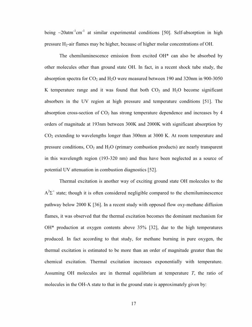
Figure 4.7. OH* mechanism validation in syngas flames at elevated pressure.

Chemiluminescence intensity ratio predictions and experimental data for

H2:CO=50:50 mixture at 10 atm and 598 K reactant preheat. .............................. 64

Figure 4.8. CO2*/OH* chemiluminescence intensity ratios (a) in H2:CO=50:50 (10 atm)

and H2:CO=33:67 (5 atm) mixtures, (b) at φ=0.6 for 10 atm and 598 K preheat .65

Figure 4.9. Measured and simulatated normalized chemiluminescence for (a) OH* and

(b) CO2* for a H2:CO=50:50 syngas mixture at 10 atm and 598 K reactant

preheat. .................................................................................................................. 66

Figure 4.10. Measured and simulated normalized chemiluminescence at φ=0.6 for (a)

OH* and (b) CO2* in H2:CO syngas mixtures with 40%, 50%, 60% and 80%

Hydrogen, at 10atm and 598 K reactant preheat conditions. ................................ 67

Figure 5.1. Simulation results of normalized integrated heat release rate, normalized

integrated OH* and CO2* chemiluminescence signal profiles. ............................ 74

Figure 5.2. OH* model validation: chemiluminescence intensity ratio predictions in (a)

swirl combustor and (b) laminar methane flames at p=1 atm and 298 K. ............ 76

Figure 5.3. Comparison between measured and simulated normalized chemiluminescence

for a) OH* emission and b) CO2* emission in methane flames............................ 79

Figure 5.4. Comparison between experimental results and model predictions for a)

CH*/OH* chemiluminescence intensity ratio and b) normalized CH* emission in

methane flames at 1 atm and 298 K. ..................................................................... 84


integrated OH* and CO2* chemiluminescence signal profiles in a methane flame

at 10 atm and room temperature conditions. The equivalence ratio is 0.8............ 87

xiii

Figure 5.6. Chemiluminescence image analysis for a methane flame at 10 atm, 298 K and

φ=0.97. (a) Raw image (burner diameter is 6 mm) and b) radial (line of sight)

Intensity profiles from the burner center axis, at 20% and 80% of the flame

height. .................................................................................................................... 89

Figure 5.7. OH* model validation in methane flames at elevated pressure conditions:

chemiluminescence intensity ratio predictions for flames at p=10 atm and 298 K.

............................................................................................................................... 90

Figure 5.8. OH* mechanism validation in methane flames at elevated pressure

conditions: (a) normalized OH* emission and (b) CO2* emission for flames at

10 atm and 300 K reactants. .................................................................................. 91

Figure 5.9. CO2*/OH* chemiluminescence intensity ratios in methane flames at elevated

pressure. Experimental data represented by symbols and simulation results

depicted by lines: dashed line for 5 atm-298 K cases, dot dashed line for 5 atm-

598 K case and solid line for 10 atm-298 K case.................................................. 92

Figure 5.10. Normalized chemiluminescence signals in methane flames at elevated

pressure: (a) OH* emission and (b) CO2* emission. Experimental data

represented by symbols and model predictions depicted by lines: dashed line for 5

atm-298 K cases, dot dashed line for 5 atm-598 K case and solid line for 10 atm-

298 K case. ............................................................................................................ 93

Figure 5.11. Spectral shape of the CO2* continuum in methane flames at various pressure

conditions at φ~075. .............................................................................................. 94

Figure 5.12. OH* and CO2* model predictions with San Diego (lines) and GRI Mech 3.0

(lines with symbols) reaction mechanisms in methane air flames at various

pressure and temperature conditions. .................................................................... 95

Figure 5.13. Comparison between experimental results and simulations for (a) CH*/OH*

chemiluminescence intensity ratio and (b) normalized CH* emission in methane

flames at 10 atm and 298 K................................................................................... 96

Figure 5.14. Validation of CH* chemiluminescence model in methane flames at elevated

pressure: (a) CH*/OH* intensity ratio and (b) normalized CH*

chemiluminescence signal. Experimental data represented by symbols and model

predictions depicted by lines: dashed line for 5 atm-298 K cases, dot dashed line

for 5 atm-598 K case and solid line for 10 atm-298 K case.................................. 97

Figure 5.15. CH* model predictions with San Diego (lines) and GRI Mech 3.0 (lines with

symbols) reaction mechanisms in methane air flames at various pressure and

temperature conditions. ......................................................................................... 99

Figure 5.16. Nominal “CO2* background” spectral shape in typical premixed flames of

syngas mixtures, methane and Jet-A fuels at atmospheric pressure conditions.. 103

xiv

Figure 5.17. Comparison between measured and simulated normalized

chemiluminescence for a) OH* emission and b) CH* emission in Jet-A flames.

............................................................................................................................. 104

Figure 5.18. CH*/OH* chemiluminescence intensity ratio variation with equivalence

ratio in a premixed, prevaporized and preheated (450K) Jet-A flame at 1 atm. . 106

Figure 6.1. Spatially integrated OH* chemiluminescence in syngas (H2:CO=50:50)

flames at various pressure and temperature conditions....................................... 110

Figure 6.2. Spatially integrated OH* chemiluminescence in methane flames at various

pressure and temperature conditions. .................................................................. 112

Figure 6.3. Comparison between the volumetric photon emission rate (iOH*) for OH*

produced by R1 and R3, in a methane-air flame at 5 atm, 700 K (φ=0.8). ......... 113

Figure 6.4. Comparison between the volumetric photon emission rate (iCH*) for CH*

produced by R6 and R7, in methane-air flame at 5atm, 700 K (φ=0.8).............. 116

Figure 6.5. Normalized spatially integrated CO2* chemiluminescence in H2:CO=50:50

syngas mixture at various pressure and temperature conditions (φ=0.8). ........... 118

Figure 6.6. Variation of (a) OH*, (b) CO2* chemiluminescence with equivalence ratio at

various pressure and preheat conditions.............................................................. 121

Figure 6.7. Strain rate dependence of OH* (solid lines) and CO2* (symbols on lines)

chemiluminescence in H2:CO=50:50 syngas mixture......................................... 123

Figure 6.8. Dependence of OH* (solid lines) and CO2* (symbols on lines)

chemiluminescence on product recirculation in a H2:CO=50:50 (φ=0.7) syngas

mixture. ............................................................................................................... 126

Figure 6.9. OH* chemiluminescence in methane at various pressure and preheat; the high

pressure results are scaled to the right axis. ........................................................ 128

Figure 6.10. CH* chemiluminescence in methane at various pressure and preheat

conditions. ........................................................................................................... 129

Figure 6.11. Strain rate dependence of OH* (lines) and CH* (lines with symbols)

chemiluminescence in methane-air flames at φ=0.7. .......................................... 131

Figure 6.12. Strain rate dependence of OH* chemiluminescence produced via R1 (lines)

and R3 (lines with symbols) in methane-air flames (φ=0.7). .............................. 132

Figure 6.13. Strain rate dependence of CH* chemiluminescence produced via R6 (lines)

and R7 (lines with symbols) in methane-air flames (φ=0.7). .............................. 133

xv

Figure 6.14. Dependence of OH* (solid lines) and CH* (lines with symbols)

chemiluminescence on product recirculation in methane-air flames (φ=0.7). .... 134

Figure 6.15. Variation of the CO2*/OH* chemiluminescence ratio with equivalence ratio

at various pressure and preheat conditions. The atmospheric results are scaled

with the left axis; the rest of the data scale with the right axis. .......................... 137

Figure 6.16. CH*/OH* chemiluminescence ratio in methane-air flames at various

pressures and preheat; the high pressure results are scaled to the right axis....... 139

Figure 6.17. Dependence of CH*/OH* ratio with strain rate for φ=1 (dashed line) and φ

=0.7 (solid line). .................................................................................................. 140

Figure 6.18. CO2* contribution in methane flames to OH*(309±5nm) and CH*

(431±5nm) signals; (a) atmospheric pressure and (b) elevated pressure. ........... 144

Figure 6.19. Comparison of chemiluminescence intensity ratio for CH* and OH*: with

background correction (closed symbols); without background correction (open

symbols). ............................................................................................................. 146

Figure 6.20. Variation of normalized (a) OH* and (b) CH* chemiluminescence signals at

elevated pressure conditions. Background corrected signals (closed symbols) and

uncorrected signals (open symbols). ................................................................... 146

Figure 7.1. Normalized CH* chemiluminescence in oxy-methane flames at atmospheric

pressure and temperature. Suggested approach for differentiating CH*

chemiluminescence mechanisms. Oxidizer is an equi-molar mixture of O2 and N2.

............................................................................................................................. 154

Figure B.1. Relative spectral responsivity of the spectrometer-ICCD camera detector

system. Theoretical (lines); Experiments (symbols). .......................................... 160

xvi

SUMMARY

Naturally occurring flame chemiluminescence, the radiative emission from

electronically excited species that are formed in chemical reactions, has received

increasing attention for its potential sensor and diagnostic applications in combustors.

Since these species are mainly produced in the reaction zone, chemiluminescence can be

indicative of the reacting conditions in the flame. A number of studies have used flame

chemiluminescence to monitor flame status, and combustor performance. Most of these

studies have been experimental, with the relationship between the chemiluminescence

and the combustion state determined empirically. However, chemiluminescence

modeling has the potential to provide a better understanding of the chemiluminescence

processes and their dependence on various combustion operating conditions.

The primary objective of this research was to identify and validate the important

chemiluminescence reaction mechanisms for OH*, CH* and CO2*. To this end,

measurements were performed at various operating conditions, primarily in laminar,

premixed flames, fueled with methane, syngas (H2/CO) and Jet-A. The results are

compared to 1-d laminar flame simulations employing the chemiluminescence

mechanisms. The secondary objective was to use the experiments and validated

chemiluminescence reaction mechanisms to evaluate the usefulness of flame

chemiluminescence as a combustion diagnostic, particularly for heat release rate and

equivalence ratio.

The validation studies were able to identify specific mechanisms for OH*, CH*

and CO2* that produced excellent agreement with the experimental data in most cases.

xvii

The mechanisms were able to predict the variation of the chemiluminescence signals with

equivalence ratio and, in most cases, preheat but not the variation with pressure. This is

attributed in part to inaccuracies in the basic chemical mechanism used in the simulations

to predict concentration profiles of the chemiluminescence precursor species. For CH*,

lack of accurate quenching data may also contribute. For OH*, thermal excitation and

radiative trapping may also be problematic at high pressure, especially near

stoichiometric conditions. For CO2*, trapping and interference from the emissions of

other species (such as HCO and H2O) lead to discrepancies between experiments and

simulations at high pressure and in Jet-A flames.

Regarding the utility of chemiluminescence for sensing, a number of observations

can be made. It is advisable to use background subtracted chemiluminescence signals for

sensing purposes. In syngas-air flames, CO2* is a reasonable heat release rate marker, at

least for very lean conditions, as it is less dependent on equivalence ratio than OH*. For a

similar reason, OH* shows some advantage in atmospheric-pressure methane and Jet-A

flames in general, while CH* is advantageous at high pressure and very lean conditions at

atmospheric pressure. The chemiluminescence intensity ratio CO2*/OH* is not useful for

sensing equivalence ratio in syngas flames, except maybe at very lean conditions.

However, the CH*/OH* signal ratio is a promising approach for sensing equivalence

ratio at low or very high pressure conditions in hydrocarbon flames. Thermal excitation

and self-absorption processes for OH* chemiluminescence can become important for

combustors operating at high pressure, high preheat and near stoichiometric conditions.

1

CHAPTER 1

INTRODUCTION

1.1 Motivation

Monitoring and controlling combustor performance and health is a major

challenge because of the harsh environment within the combustor. For understanding

combustion and ocmbustors, the spatial and temporal distribution of parameters such as

temperature, pressure, equivalence ratio, heat release rate and pollutant levels are of great

interest. Robust and reliable diagnostic and sensor systems are even more relevant to

future combustors due to the many issues facing modern lean, premixed combustors and

the fuel-flexible versions under development. For example in lean premixed combustors,

monitoring and control of the combustor operating point is necessary to harness the full

benefits of NOx reduction. That these combustors operate near the lean stability limit

with the flame more prone to blowout and combustion dynamics further motivates the

need for robust control and sensing methodologies. To this end, optical methods have

become a popular choice because the measurements are non-intrusive and there are

optical interface materials can survive the high temperatures combustor environment.

Optical sensors have the added advantage of being quite fast and capable of giving both

localized and global information about the combustion process. The fast response of

these sensors is particularly useful in monitoring dynamic processes in combustion

systems. However, most of the quantitative methods are laser-based, with higher costs,

complexity, and maintenance requirements.

2

Flame chemiluminescence has received renewed attention for its potential sensor

applications in combustors. The radiative emissions from electronically excited species

that are formed chemically, such as CH*, OH*, C2* and CO2* constitute the primary

sources of chemiluminescence in hydrocarbon flames [1]. Since these species are mainly

produced in the reaction zone, chemiluminescence can be indicative of the reacting

conditions in the flame. This idea has led many to explore the use of flame

chemiluminescence in practical combustors to monitor flame status, and combustor

health and performance. For example, chemiluminescence imaging of excited radicals, an

obvious application, is often used for reaction zone marking [2, 3]. Similarly, the ratio of

emissions from excited species, such as CH*/OH* or C2*/OH

*, show promise for

equivalence ratio sensing in both gaseous and liquid fuel systems [4]. For example, it has

0.5 0.6 0.7 0.8 0.9 10

0.2

0.4

0.6

0.8

φφφφ

CH*/OH*

Re = 11700

Re = 14900

Re = 18700

Re = 23300

Figure 1.1. Variation of CH*/OH

* chemiluminescence intensity ratio on equivalence

ratio for various inlet axial Re in a swirl combustor [4].

3

been observed that the ratio of CH*/OH* peak intensities monotonically increases with

equivalence ratio in methane flames at atmospheric conditions (Figure 1.1) [4], and hence

could be used for sensing equivalence ratio at these conditions. Chemiluminescence has

also been employed to characterize temporal fluctuations in global heat release rate and

its spatial distribution for applications related to combustion instabilities [5].

Nevertheless, most of these studies have been experimental, with the relationship

between the chemiluminescence and the combustion state determined empirically. Thus

the relationship between chemiluminescence signals and combustion parameters must be

experimentally revisited whenever the operating conditions change in a significant way.

Chemiluminescence modelling on the other hand has the potential to provide a better

understanding of the chemiluminescence processes and their dependence on various

combustion operating conditions. Modeling provides better control for isolating and

studying the conditions of interest compared to experiments. Modeling can also be

helpful in designing a diagnostic or sensing approach, and interpreting experimental

results. The success of the model mainly depends on the accuracy of the reaction

mechanisms for the formation of the excited-state species and the associated reaction

rates, assuming that the chemiluminescence precursor species are well-estimated by

standard combustion models for the particular fuel-oxidizer system of interest. Thus,

most of the earlier modeling efforts were intended to identify the chemiluminescence

reactions and their rates [6,7] or to understand the relationship between

chemiluminescence and flame properties [8,9] using proposed chemiluminescence

mechanisms that were not systematically validated. Additionally, these studies examined

OH*, CH

* and C2

* primarily in methane-air flames. In the case of CO2

*

4

chemiluminescence, its relevance to determination of flame properties such as heat

release in laminar and turbulent premixed flames was evaluated by Samaniego et al. [10]

via a numerical investigation without experimental validation using outdated rate

constant information for CO2* chemiluminescence.

Thus, the objective of this thesis is to identify and validate the important

chemiluminescence reactions for OH*, CH* and CO2* and to study the dependence of

flame chemiluminescence on combustion parameters such as pressure, reactant preheat,

equivalence ratio, strain and the degree of reactant/product mixing for a range of relevant

fuels: methane, syngas and Jet-A. Thus the proposed work will provide direction on the

potential sensor applications of flame chemiluminescence. Methane and syngas fuels

were chosen in part because of the availability of validated mechanisms, such as GRI

Mech 3.0, and because of the extensive application of natural gas in industrial

applications, and the great interest in syngas and CH4/H2 mixtures for future applications.

Jet-A was chosen due to its importance in aircraft engines, and because it involves a

significant increase in fuel-chemistry complexity over the other choices.

1.2 Literature Review

Equivalence ratio is one of the important engine parameters that needs to be

monitored and controlled both globally and locally, for variations in fuel-air ratio could

lead to undesirable consequences such as increased NOx and soot emissions, reduced

flame stability and ultimately combustor (acoustic) instabilities that may be detrimental

to the .structural integrity of the combustor itself. In this regard, a number of studies in

the 1950’s [11-13] have laid the foundation for sensing this important parameter among

others (such as heat release rate) using flame chemiluminescence. For example, Clark

5

[13] investigated the dependence of chemiluminescence signals of OH*, CH*, C2* and

CO2* on fuel type, flow rate and equivalence ratio. It was showed that the ratio of

C2*/CH* chemiluminescence signal intensities could be used for monitoring equivalence

ratio in propane-air and ethylene-air flames. Recent studies in both premixed and

partially premixed gaseous and liquid fuel systems [4, 14-19] have strengthened the

promise for equivalence ratio sensing via ratio of emissions such as CH*/OH* or

C2*/OH

*. However, these studies only reported empirical correlations for a specific

burner and detection system, which may not be generally applicable. Additionally, most

of the studies considered flows with simultaneous variations of strain rate, temperature or

pressure in addition to equivalence ratio, further limiting the relevance of the findings.

Chemiluminescence emission from OH*, CH*, CO2* and C2* have been studied

in laminar and turbulent flames, and since the early days it was assumed to be a marker

and measure for heat release rate [13]. This was due to the observation that radiation

intensity increased linearly with fuel flow rate in both laminar and low-intensity turbulent

flames, for other conditions fixed, e.g., at a given equivalence ratio or reactant

temperature. This assumption was further strengthened by the work of Price et al. [20]

and Hurle et. al [21] in ethylene-air, turbulent, premixed and diffusion flames when they

observed excellent correlation between the time derivative of the C2* and CH*

chemiluminescence light signal strength and the root mean square pressure, as measured

by a microphone some distance away from the flame. Subsequent studies used this

hypothesis without additional evaluation of the influence of combustion parameters (i.e.,

equivalence ratio, pressure, temperature, and flame strain rate) on the chemistry of the

excited radicals leading to chemiluminescence and its potential link to heat release [22,

6

23]. This correlation between chemiluminescence rate and acoustic pressure was later

verified in laminar flames in steady and unsteady combustion under moderate strain, for

fixed conditions such as equivalence ratio, pressure, temperature, and flame strain rate

[10,,25]. However in highly turbulent flames or regions with extreme local strain or flame

curvature, chemiluminescence can effectively go to zero without flame extinction [26-

28]. Hence, the assumption severely fails in such situations and flame

chemiluminescence would not be reliable for heat release rate marking.

Thus while flame emission has been used to characterize temporal fluctuations

both in overall heat release rate and the spatial distribution of local heat release rate

[5,29], care must be taken when interpreting such measurements. For example, when

making overall chemiluminescence measurements, it is important to realize that changes

in the fuel flow rate and changes in the equivalence ratio independently affect the overall

chemiluminescence emission. So, it can be necessary to measure both fuel flow rate and

equivalence ratio oscillations to get accurate information about the phase and amplitude

of the overall heat release rate fluctuations [28].

As noted previously, these relationships could be studied in detail if validated

mechanisms for OH*, CH* and CO2* chemiluminescence were available. The required

mechanism should account for the formation and destruction of the excited state species.

There has been considerable work identifying the formation reactions and their rate

parameters for OH* and CH*. For these two species, there have been a number of

experimental studies in premixed methane air systems including some at high pressure

[19,,31] and with purposefully applied strain [30,24]; yet few have focused on validating

the chemiluminescence mechanisms [32]. In addition, most of these studies were limited

7

to methane-air mixtures and room temperature conditions. In summary, there is a need

for a parametric study over a range of operating conditions such as fuel type, reactant

temperature, pressure, dilution, strain, and equivalence ratio on the behavior of flame

chemiluminescence, and its relation to heat release rate and equivalence ratio. Such a

study would help provide insight into the dependence of chemiluminescence on these

parameters and improve interpretation of experimental data.

1.3 Overview of Present Work

The main objective of this thesis is to develop a predictive model for flame

chemiluminescence from three sources: OH*, CH* and CO2*. The secondary objective is

to use the validated chemiluminescence reaction models to evaluate the usefulness of

flame chemiluminescence as a combustion diagnostic at various operating conditions for

gaseous and liquid fuels of importance: viz. methane, syngas and Jet-A.

The approach taken to accomplish the first objective is to evaluate mechanisms

and rates identified in the literature for OH*, CH* and CO2* by comparing the global

chemiluminescence yield measured in flame experiments to that predicted by the models.

Identifying the appropriate mechanisms includes a literature review of the proposed

chemiluminescence formation reactions and their associated rate parameters, as well as

identification of the important collisional quenchers and their corresponding rate

parameters. For the verification task, it is essential to perform experiments at a range of

controlled operating conditions, including: pressure, reactant preheat temperature,

equivalence ratio and reactant dilution. The studies are primarily carried out in simple

laminar premixed flames, which provide a well-controlled environment for measuring

global flame chemiluminescence. They are also more amenable to simulation. Then, the

8

chemiluminescence models are validated by comparing the experiments to simulation

results. The simulations are performed for unstrained laminar flames with leading

chemical kinetic mechanisms relevant to the above fuels, and the global

chemiluminescence yield is calculated using the available chemiluminescence reactions

and their rates. The approach to the second objective involves using the validated

chemiluminescence models to study the dependence of flame chemiluminescence on

combustion parameters such as pressure, reactant preheat, strain equivalence ratio and

degree of reactant/product mixing in the above fuels.

The general thesis outline is as follows: Chapter 2 provides necessary background

information about flame chemiluminescence and chemiluminescence mechanisms for

OH*, CH* and CO2* excited species including their formation reactions and quenching

reactions with their associated rate parameters from the literature. Chapter 3 describes the

experimental facilities used in this study, including the burners and the optics necessary

for acquiring flame chemiluminescence. Additionally, details of the chemiluminescence

modeling approach used to estimate global chemiluminescence yield from the flames are

presented in this chapter. The comparisons between the model predictions and

experiments are made in Chapter 4 and the most appropriate models are evaluated for

OH*, CH* and CO2* chemiluminescence. The validated models are then used in Chapter

5 to evaluate flame chemiluminescence from these species, for sensing equivalence ratio

and heat release rate in premixed flames of a representative syngas mixture and methane

at various operating conditions. This chapter also provides estimates of the contribution

of thermally produced OH* to the total OH* signal in these flames. The chapter also

examines the implications for chemiluminescence sensing if total signals are considered,

9

without background subtraction, simulating chemiluminescence acquired by “single”

wavelength detection systems. Finally, Chapter 6 concludes the thesis with a summary

and recommendations for further studies.

10

CHAPTER 2

BACKGROUND

This chapter provides a brief overview of chemiluminescence and the reaction

mechanisms responsible for it. In particular, formation reactions, quenching reactions and

their appropriate rate parameters established in the literature are presented for OH*, CH*

and CO2*.

2.1 Chemiluminescence

Chemiluminescence, as the name suggests, is the light that is produced as a result

of chemical reaction. In other words, it is the spontaneous electromagnetic radiation that

is produced when chemically created excited states return to a lower energy state (ground

state generally) [1]. Chemiluminescence forms a part of the wider domain of emission

spectroscopy. In this thesis, flame emission mainly in the UV-VIS part of the

electromagnetic spectrum is considered. In particular, it deals with emission from the

excited molecules OH*, CO2* and CH*. Emission in the visible and ultra-violet regions

is generally due to changes in electronic states of the molecule. This change determines

the position of the molecular band system as a whole. The position of the individual

bands within the band system is determined by the changes in the vibrational energy

states of the molecule. The fine line structure of the band (fine structure of the individual

bands) on the other hand is determined by the changes in the rotational energy states

within the molecule.

11

The net photon emission due to chemiluminescence from an excited molecule

(say OH*) depends on the following steps as illustrated in Figure 2.1: 1) excited state

formation via chemical reactions (F), 2) excited state formation via thermal excitation

(T), 3) (rapid) collisional quenching reactions that remove the excited state, reducing to

its ground electronic configuration non-radiatively (Q), 4) reactive collision with another

molecule (R), and 5) spontaneous radiative transitions to the ground state (A).

F

X+YZ

XY*

XY

Q T A hν

R +Y X+Y2

Figure 2.1. General steps involved in a chemiluminescence reaction mechanism.

Often, the whole process is dominated by quenching, with the process limited by

formation of the excited state*. For these reasons, they can often be assumed to be in

quasi-steady state [10], i.e., for an excited state XY*

ARQTFdt

XYd−−−+=≈ 0

][ *

. (1)

where F and T represent the production rates of the excited state by chemical and thermal

excitation mechanisms; Q, R and A represent the removal rates of the excited state by

collisional quenching, reactive quenching, and by spontaneous emission. Thus the

* This leads to low concentrations for the electronically excited species, which then have little impact on the

overall flame chemistry.

12

concentration of the excited state, [XY*], can be estimated from Eq. (1). The

chemiluminescence photon production rate is given by

][][ *XYA

dt

hvd= . (2)

The accuracy of chemiluminescence modeling directly depends on the accuracy

with which these sub-steps are modeled. All the above steps shall be considered for OH*,

CO2* and CH* chemiluminescence provided that enough information is found in the

literature.

2.2 OH* Chemiluminescence

Emission from the electronically excited OH A2Σ+

state (typically denoted OH* in

the flame chemiluminescence literature) near 310 nm is a prominent feature of hydrogen

and hydrocarbon flame spectra. OH* emission and the reactions important in OH

*

chemiluminescence have long been studied [33-37]. Collisional quenching and radiative

decay rates for OH excited states are largely well known from extensive studies of OH

photophysics [38]. For example, the overall Einstein A coefficient for the OH A2Σ+

state

is given as 1.4×106

s-1

[38]. It is the formation reactions and rates that have been more

difficult to determine.

Experimental efforts to determine the dominant OH* formation steps have

primarily taken one of two approaches: 1) flame and 2) shock-tube studies. In flat flame

studies of lean and rich (φ=1-1.5) H2/O2/N2 mixtures [34], the authors assumed partial

equilibrium among the flame radicals and were able to conclude that the following three-

body reactions were a likely source of the OH* state.

13

O + H + M → OH* + M (R1)

H + OH + OH → OH* + M (R2)

However, the equilibrium relationships between the radicals prevented the assignment of

a unique excitation mechanism for OH* formation. Shock tube studies with H2/O2/Ar

mixtures were undertaken so as to make kinetic measurements far from equilibrium.

Most of these studies [36,37,39] strongly indicated that (R1) was the main source of OH*

in hydrogen systems. Still, Smith et al. [40] suggested an optimized model taking into

account both reactions R1 and R2 for hydrogen combustion.

Many of these flame and shock tube studies also attempted to estimate the rate

constants for the OH* formation reactions. Because of the more controlled nature of the

shock tube studies, their results may be more reliable. In most of these studies, however,

the authors reported temperature independent rate constants, with the exception of one

shock tube study, where an Arrhenius type rate for R1 was reported [36]. Their rate

constant was updated in a later shock tube study [37], though without change in the

temperature dependence. It should be noted here that the experimentally determined rate

constants are mainly based on OH* chemiluminescence data acquired with detectors

coupled to filters with at least full width half maximum (FWHM) of ~10nm.

In combustion of hydrocarbon fuels, OH* formation has been most often

attributed to the four-center reaction [1,7, 41-44],

CH + O2 → OH* + CO (R3)

with rate constants also usually given without temperature dependence. Kinetic rate

parameters for this reaction were determined experimentally, primarily in flames, flow

reactors and shock tubes. Recently, the shock tube study of Hall et al. [45] was able to

14

provide information on the temperature dependence of this reaction. Table 2.1

summarizes the OH* mechanism and rate constant information, with the rate constant

parameters given in a modified Arrhenius form.

Table 2.1. Formation (R) and quenching (Q) reactions and rate constants reported

for OH*. Rate coefficients are expressed as k = A T

b exp(−−−−Ea/RT) with Ea in units of

cal mol-1 and AT

b in cm

3mol

-1s-1 for two body reactions or cm

6mol

-2s-1 for three body

reactions (with T in K units).

# Reaction A b Ea Ref.

R1 H + O + M ↔ OH* + M 6 × 1014 0.0 6940 [37]

3.1 × 1014 0.0 10,000 [45]

5.45 × 1012

[40]

3.63 × 1013

[43]

1.2 × 1013 0.0 6940 [36]

R2 H + OH + OH ↔ OH* + H2O 1.45 × 1015

[40]

R3 CH + O2 ↔ OH* + CO 3.24 × 1014

-0.4 4150 [45]

1.8 × 1011

[43]

3.72 × 1010

0 167.2 [44]

Q1OH OH* + H2O → OH + H2O 5.92 × 1012

0.5 -861 [38]

Q2OH OH* + CO2 → OH + CO2 2.75 × 1012 0.5 -968 [38]

Q3OH OH* + CO → OH + CO 3.23 × 1012 0.5 -787 [38]

Q4OH OH* + H2 → OH + H2 2.95 × 1012 0.5 -444 [38]

Q5OH OH* + O2 → OH + O2 2.10 × 1012 0.5 -482 [38]

Q6OH OH* + OH →OH + OH 1.50 × 1012 0.5 0.0 [36]

Q7OH OH* + H → OH + H 1.50 × 1012 0.5 0.0 [36]

Q8OH OH* + O → OH + O 1.50 × 1012 0.5 0.0 [36]

Q9OH OH* + N2 → OH + N2 1.08 × 1011 0.5 -1238 [38]

Q10OH OH* + CH4 → OH + CH4 3.36 × 1012

0.5 -635 [38]

It can be seen from Table 2.1 that the R1 rate constant (k1) reported in. the

literature at 1800K varies from 1.72×1012

to 8.62×1013

cm3/mol⋅s, i.e., a variation of

approximately 50 times. However, if the most recent rates for R1 are considered, k1

would vary less, between 5.45×1012

and 8.62×1013

at 1800 K. Nevertheless, k1 given in

[40] should not be considered as it was lowered to accommodate the contribution of R2

15

in that study. So, finally k1 would just vary by ~3 times from 3.63×1013

to 8.62×1013

at

1800 K, if only recent rates for R1 are considered. Similarly, it can be seen that the rate

constant of R3 as reported in literature varies from 3.55×1010

to 5×1012

cm3/mol⋅s at

1800 K. It should be noted that the discrepancy in the absolute rate constant of R1 is

lesser than that of R3.

Another important difference between the models is the activation energy

assigned for the reactions R1 and R3, which directly impacts the temperature dependence

of the reaction rate constants. It should be noted, however, that the activation energy for

R1, cited by the various sources is not very high. This implies that the reaction rate

constant has weak temperature dependence except at low temperatures (for example,

found in flames of lean equivalence ratios). The same is applicable for R3 also.

Table 2.1 also lists the primary quenching collisions in simple H2/CO/CH4 flames.

In lean methane flames with air as the oxidizer, H2O is the most effective quencher, while

CO, CO2 and O2 are also important. However, in complex fuel systems such as Jet-A,

there might be other quenchers such as alkanes, alcohols and aromatics as they are large

molecules that may have significant quenching cross-sections. However, there is little

research regarding the OH* quenching rates by these molecules. Another path of

destruction of OH*, by chemical reaction, is possible. For example, in the case of H2 [46-

48],

OH* + H2 → H + H2O

Experiments have shown that break up of the OH(A2Σ

+)-H2 Van der Waals cluster

produced a significant yield of H atoms [47]. In fact, most recent results conclude that

only a small fraction of the products, less than 15%, arise from nonreactive quenching

16

while reactive quenching is the dominant product channel [48]. This approach is expected

to be applicable to the collisional quenching of OH* by other partners (H2O, CO2 etc.)

and for collisional quenching of other excited state species (for example, CH*) as well.

The authors speculate that reactive quenching may be the norm in collisional quenching

processes with large cross sections (H2O etc.) [48]. However to date, reactive quenching

of OH* is considered only for H2 while few older studies have termed this pathway

insignificant [43]. This aspect of quenching is not considered in this thesis due to lack of

sufficient information.

Absorption of the emitted photon by another ground state OH molecule before it

reaches a detector is indirectly related to the whole process and can be estimated using

the Beer-Lambert relation given by [49,50],

−= ∫ ν

l

OH

o

dlpXkI

I

0

exp . (3)

where kv is the spectral absorbance coefficient, p is the pressure, XOH is the absorbing OH

mole fraction and l is the absorbing path length. The absorption coefficient, kv, is a

function of temperature and pressure [49]. It can be seen from Eq. 3 that the absorption is

maximum when the product pXOHl is maximum. A numerical study in methane-air flames

shows that this case corresponds to atmospheric pressure and near-stoichiometric

conditions [31]. In methane-air premixed laminar flames at room temperature for

different operating pressures (1-10 atm), the self-absorption was estimated to be a

maximum of ~15% by the same authors [31], with the maximum absorption coefficient

per unit pressure per unit length in the R-branch bandhead of the OH A-X (0,0) band

17

being ~20atm-1

cm-1

at similar experimental conditions [50]. Self-absorption in high

pressure H2-air flames may be higher, because of higher molar concentrations of OH.

The chemiluminescence emission from excited OH* can also be absorbed by

other molecules other than ground state OH. In fact, in a recent shock tube study, the

absorption spectra for CO2 and H2O were measured between 190 and 320nm in 900-3050

K temperature range and it was found that both CO2 and H2O become significant

absorbers in the UV region at high pressure and temperature conditions [51]. The

absorption cross-section of CO2 has strong temperature dependence and increases by 4

orders of magnitude at 193nm between 300K and 2000K with significant absorption by

CO2 extending to wavelengths longer than 300nm at 3000 K. At room temperature and

pressure conditions, CO2 and H2O (primary combustion products) are nearly transparent

in this wavelength region (193-320 nm) and thus have been neglected as a source of

potential UV attenuation in combustion diagnostics [52].

Thermal excitation is another way of exciting ground state OH molecules to the

A2Σ+

state; though it is often considered negligible compared to the chemiluminescence

pathway below 2000 K [36]. In a recent study with opposed flow oxy-methane diffusion

flames, it was observed that the thermal excitation becomes the dominant mechanism for

OH* production at oxygen contents above 35% [32], due to the high temperatures

produced. In fact according to that study, for methane burning in pure oxygen, the

thermal excitation is estimated to be more than an order of magnitude greater than the

chemical excitation. Thermal excitation increases exponentially with temperature.

Assuming OH molecules are in thermal equilibrium at temperature T, the ratio of

molecules in the OH-A state to that in the ground state is approximately given by:

18

( ) )000,47exp(5.0 TKNNtotOHAOH −= . (4)

With this approximation, the thermal [OH*] profile, and subsequently the spontaneous

emission from this OH-A state can be calculated in the flames.

2.3 CO2* Chemiluminescence

The origin and structure of the CO2* “blue continuum” emissions (because most

of the light emitted is in the blue region of the electromagnetic spectrum) have also been

investigated by various groups. However, its mechanism is probably the least understood

when compared to OH* and CH* chemiluminescence. In early studies with H2/CO/O2

flames, shock tubes, and flow reactors, researchers found that the emission intensity was

proportional to the product of [CO] and [O] concentrations and concluded that a reaction

similar to (R4) was the primary cause of CO2* chemiluminescence [53].

CO + O → CO2* (R4)

Later in a series of low temperature, flow reactor studies, Pravilov et al. [54] identified

the likely states involved in CO2* chemiluminescence.

CO(X1Σ

+) + O(

3P) → CO2(

3B2)

CO2(3B2) → CO2(

1B2)

CO2(1B2) → CO2(X

1Σ

+g) + hv

CO2(1B2) + M → CO2(X

1Σ

+g) + M

First an intermediate excited triplet state of CO2 is formed with the reaction of CO and O

in their electronic ground states. The triplet state then rapidly transitions to an excited

singlet state. The combination of these two steps is equivalent to (R4). The radiative de-

excitation of the single state produces the CO2* chemiluminescence, with the radiative

decay competing with collision quenching reactions. It is through the first step that the

19

emission rate becomes dependent on the concentrations of [CO] and [O]. This study also

found that the CO2* continuum has a spectral shape that changes only slightly over a

range of temperatures.

None of these studies investigated the individual rates for the detailed CO2*

mechanism described above and further systematic research has to be done to investigate

the effect of various collider molecules such as H2O and CO2 on CO2*

chemiluminescence. However, one study claims that collisional quenching of CO2*

chemiluminescence with O2 is highly temperature dependent and the quenching

efficiency decreased by a factor of 35 as temperature increased from 206 to 353 K , and

becomes negligible at flame temperatures [54]. Hence, rate constant data have only been

reported for the overall rate of chemiluminescence emission at different temperatures and

wavelengths. The most recent work is the shock tube study in H2-CO mixtures and

review of previous work by Slack et al. [55]. They obtained spectrally resolved emission

intensities for wavelengths from 250-700 nm and in the temperature range 1300-2700 K.

It should be noted that for higher temperatures, interferences to the CO2* continuum

emission at wavelengths below 450 nm have been seen in carbon monoxide/oxygen

systems due to the radiative combination of oxygen atoms and by the radiation resulting

from the electronic excitation of O2 [56].. Moreover, a similar scenario is possible in

hydrocarbon flames where emission from other molecules such as HCO, H2O can overlap

with the UV-VIS continuum [57-59] and the CO2* chemiluminescence signal may be

corrupted. As in the earlier study by Pravilov, Slack et al. found only a weak dependence

of the spectral shape of the continuum emission on the temperature. Using these results,

20

they determined the spectrally integrated rate expression for the CO2* chemiluminescence

volumetric photon emission rate (in moles of photons),

scm

molOCO

T

KiCO ⋅

−×=

3

5 ]][][1950

exp[108.6*2

(5)

They also showed that this expression extrapolates well to the low temperature data of

Pravilov. The magnitude and temperature dependence of this expression is different than

the earlier results summarized in [53], which were used in a previous CO2* modeling

study [10].

2.4 CH* Chemiluminescence

The primary CH* emission in the UV-VIS region is due to the A2∆→X

2Π (at

~431nm) and B2Σ-→ X

2Π (~390nm) transitions, with the 431 nm band usually

dominating [1]. As was the case with OH*, the CH* chemiluminescence mechanism

requires: 1) excited state formation reactions and their rates, and 2) collisional quenching

and radiative relaxation rates that remove the excited state. Radiative rates and quenching

data for CH* by major species of hydrocarbon combustion are available [38], though the

quenching information is not as accurate as that for OH*. Various efforts have explored

the CH* formation reactions and their corresponding rate parameters. Of the various

proposed sources, research has focused on the following.

C2 + OH → CH* + CO (R5)

C2H + O → CH* + CO (R6)

C2H + O2 → CH* + CO2 (R7)

21

Gaydon [1] suggested reaction R5; this was later challenged, first by Brenig [60]

and later by Grebe and Homann [61]. Brenig's experiments suggested that CH* formed

from the reaction of ground state ethynyl radicals (C2H) with O atoms, which had been

proposed earlier [62]. A recent shock tube study with methane-hydrogen mixtures

supports R5 and R6 as the dominant CH* formation pathways for conditions in the range

1200-2300K and 0.6-2.2 atm [63], though with large uncertainties in the rate parameters

due to inadequate information on C2 kinetics. R5 may also be important in high order

hydrocarbon (liquid) fuel systems where C2 is relatively more abundant. Devriendt et al.

[64] in a pulsed laser photolysis study at low pressure determined the temperature

dependence of R6 and concluded that the majority of CH* is produced by that reaction.

Moreover, it was demonstrated that addition of excess O2 actually decreased the CH*

yield in the pulsed laser photolysis [64] and the shock tube studies [63], which eliminated

the O2 step (R7) in the analysis.

However, Renlund et al. [65] suggested the importance of C2H with O2 rather

than atomic oxygen (R6). In a recent flash photolysis study of acetylene at low pressure

[66], the temperature dependence of R7 was evaluated; additionally the study concluded

that R7 could contribute significantly to CH* chemiluminescence in hot flames and under

fuel lean conditions. Absolute excited state concentrations of CH* were measured in low

pressure methane-air premixed flames, and rate parameters for R6 and R7 were

determined [7] and recently reanalyzed [40]. The R6 rate constant was found to be

temperature independent, while R7 showed weak temperature dependence.

In this study, four models proposed in the literature (designated by the last author

of the reference source) were used to model CH* formation in methane and Jet-A flames.

22

Each is based on two of the formation reactions (R5-R7); the reaction rate parameters

associated with each are listed in Table 2.2.

Table 2.2. Chemiluminescence reaction mechanism to model CH* formation. Rate

coefficients are expressed as k=ATbexp(-Ea/RT) with Ea in units of cal mol

-1 and AT

b

in cm3mol


6mol

-2s-1 for three body reactions (with T

in K units). Einstein A coefficient for CH* is 1.85××××106 s-1[38].

# Reaction A b Ea Ref

R5 C2 + OH ↔ CH* + CO 2 × 1014 0 0 [63]

R6 C2H + O ↔ CH* + CO 2.5(±0.8) × 1012 0 0 [40]

5.2 × 1011

0 2600 [63]

1.08(±0.4) × 1013

0a 0 [64]

6.023(±3.0) × 1012

0 457 [66]

R7 C2H + O2 ↔ CH* + CO2 3.2(±1.0) × 1011

0 1599 [40]

2.17(±0.8) × 1010

0 0 [64]

6.023 × 10-4

4.4 -2285 [66]

Q1CH CH* + H2O ↔ CH +

H O 5.3 × 10

13 0 0 [38]

Q2CH CH* + CO2 ↔ CH + CO2 2.41 × 10-1

4.3 -1694 [38]

Q3CH CH* + CO ↔ CH + CO 2.44 × 1012

0.5 0 [38]

Q4CH CH* + H2 ↔ CH + H2 1.47 × 1014

0 1361 [38]

Q5CH CH* + O2 ↔ CH + O2 2.48 × 106 2.14 -1720 [38]

Q6CH CH* + N2 ↔ CH + N2 3.03 × 102 3.4 -381 [38]

Q7CH CH* + CH4 → CH + CH4 1.73 × 1013

0 167 [38]

From the data listed in Table 2.2, the R6 rate constants (k6) reported in the

literature varies from 2.5−10.8×1012

cm3/mol⋅s at 1800K, i.e., by approximately 4 times.

Similarly, the rate constant of R7 as reported in the literature varies from

2.17−24×1010

cm3/mol⋅s at 1800 K, by approximately 10 times. It should be noted that

the discrepancy in the absolute rate constant of R6 is less than that of R7. It is also

interesting to note that the ratio of rate constants (k6/k7) has a large variation, from 12 to

500 at 1800 K. For two of the models [40, 64], the ratio (k6/k7) is almost constant while it

decreases by a factor of four in the other model [66] in the temperature range 1400-

23

1900 K. This has a direct bearing in the relative contributions of R6 and R7 to the CH*

chemiluminescence yield.

Table 2.2 also lists the primary collisional quenchers in simple H2/CO/CH4

flames. In lean methane-air flames, N2 is the dominant quencher of CH* while H2O and

CO2 are also important. However as noted for OH* in complex fuel systems (such as Jet-

A), large hydrocarbons may be important. Collisional quenching of excited CH molecule

by alcohols and alkane molecules was recently studied in the temperature range 297-

653 K [67]. Heptane (C7H16) and butyl alcohol (C4H9OH) were the largest alkane and the

alcohol molecules considered. It was found that the quenching rate increased with

temperature for the collisional partners studied. It was also observed that the quenching

of CH* by some molecules does not follow the Arrhenius relation, the same conclusion

as a previous study [68]. It was generally found that the quenching rate constants of

CH(A) increases with the number of carbon atoms in the alkane or alcohol molecule.

Also, the quenching rate constant of CH(A) with alkane or alcohol is an order of

magnitude higher in comparison to that of O2 [67]. Clearly, this is an important aspect

that should be considered when modeling CH* chemiluminescence in higher

hydrocarbon flames. Moreover, the CH* quenching with colliders such as N2 and H2O

that have significant concentrations in typical flames, is not very accurate [38], in spite of

a recent investigation [69]. Similarly as in the case of the OH(A) state [46-48], the

possibility of reactive quenching of CH(A) state cannot be ruled out, even though the

CH(X) state is usually found to be more reactive than the CH(A) state [70].

Unfortunately, very few studies have focused in this area of reactive quenching for CH*.

24

Absorption of the emitted photon by a ground state CH molecule is also

theoretically possible, as was with the excited OH* molecule. However, in typical flame

environments, particularly lean systems, the self-absorption mechanism is practically

insignificant due to the very low concentration of ground state CH(X) molecules and its

occurrence only in the thin reaction zone [31]. In other words, if Eq. (3) was used for

CH* self-absorption, both l and XCH are extremely small for ground state CH molecules.

Nevertheless, the emitted photons can be absorbed by other molecules such as CO2 and

H2O [51].

Another mechanism to produce CH* molecules is thermal (collisional) excitation

from ground state CH. In a recent study of opposed flow oxy-methane diffusion flames, it

was observed that the thermal excitation contributes less than 30% of the total

chemiluminescence signal [32]. However, for low oxygen content, thermal production of

excited CH (A) molecules is practically negligible. Assuming CH molecules are in

thermal equilibrium at temperature T, the ratio of molecules in the CH(A) state to that in

the ground state is approximately given by:

( ) )401,33exp( TKNNtotCHACH −= . (6)

With this approximation, the thermal [CH*] population, and subsequently the

spontaneous emission from the CH(A) state can be calculated. Nevertheless, in most

conditions, thermal excitation of ground state CH (X) is negligible compared to that

produced chemically. The reasons for this cause are identical to that cited for self-

absorption viz. very small concentrations of ground state CH molecules and its

occurrence in a narrow region of the flame. It has to be noted that unlike OH, CH does

25

not exist in the product gases for lean combustion and therefore, exists in regions of

lower temperature, which further discourages thermal CH* production.

In summary, there is a discrepancy in the information on the formation reactions

of the excited state for OH* or CH* and their associated rate parameters, with the

quenching reactions and rates known to reasonable accuracy. However for CO2*, it has to

be noted that the only quantitative model in the literature is simplified and does not

consider individual formation or quenching reactions and rates. The quasi-steady state

assumption for the excited molecules is incorporated in the chemiluminescence modeling

approach used here and presented in detail in the next chapter for OH*, CH* and CO2*

chemiluminescence modeling.

26

CHAPTER 3

MEASUREMENT AND MODELING APPROACHES

The details of the various combustors used for acquiring flame

chemiluminescence spectra and the data reduction procedure to extract CO2*, OH* and

CH* chemiluminescence signals from the raw spectrum are described in detail in the first

section of this chapter. A brief description of the modeling efforts, the leading kinetic

models considered and the procedure for comparing the experimental results with the

numerical simulation are discussed in the subsequent section. Finally, various sources of

uncertainties associated with the measurements are presented.

3.1 Experimental Setup

Experiments were conducted to validate existing chemiluminescence mechanisms

for CO2*, OH* and CH*. To check the accuracy and robustness of the different

mechanisms, experiments were systematically carried out by varying important

combustor parameters such as equivalence ratio, pressure, reactant preheat, dilution and

fuel type. Each experimental facility employed broadly consists of two subsystems: 1) the

burner and 2) the flame chemiluminescence detection system, including

collection/imaging optics and detector. The burners are further classified based on the

fuel type and the operating pressure. Based on this classification, detailed descriptions of

the experimental facilities and the data reduction procedure are presented in the following

sections.

27

3.1.1 Burners

Chemiluminescence spectra were obtained in premixed gaseous (syngas mixtures

and methane) and liquid fuel (Jet-A) systems. The gaseous fuels investigated in this study

are: 1) H2-CO syngas system and 2) methane (the primary component of natural gas). Jet-

A, a liquid fuel, is relevant in aeropropulsion. The gaseous fuels were studied at

atmospheric and elevated pressure, while the Jet-A experiments were limited to

atmospheric pressure. Descriptions of the atmospheric facilities are presented first,

followed by the elevated pressure facility.

3.1.1.1 Atmospheric Pressure

Atmospheric experiments with syngas mixtures were conducted in a facility that

was previously used for laminar flame speed measurements [71] as shown in Figure 3.1.

The desired syngas mixture is first prepared using a bank of calibrated rotameters, one for

each gas in the mixture. The fuel mixture is split into two flows after mixing thoroughly

with the desired amount of fuel passing through another rotameter (calibrated for the

particular fuel composition) and the remainder flared in a diffusion flame. Finally, the

required quantity of air is added, and the mixture goes to the burner. The burner is a

straight cylindrical stainless steel tube with an inner diameter of 4.5 mm, the length

chosen to ensure the flow is laminar and the exit velocity profile fully developed. The

rotameters used for the flow rate measurements were calibrated with a bubble flow meter

to ±1% accuracy, implying a maximum error of 2 % in equivalence ratio. To study the

effects of preheating, the reactants are heated by electrical resistance tape wound around

the burner tube. The desired reactant temperature (temporarily measured at the center of

the burner exit by a type-K thermocouple, TC1) is achieved by regulating the surface

28

temperature of the burner with a temperature controller based on the feedback of a second

thermocouple, TC2. The mixture temperature at the exit of the burner has a nearly

uniform radial profile (∆T≈3-5 K). The data presented here correspond to mixtures with

H2:CO volumetric ratios of 95:5, 50:50 and 33:67. Additionally for the H2:CO =50:50

mixture, two further cases were studied: reactant preheating to ~500K and 20% dilution

with CO2.

Mixing

H2

Pressure

gauge

Premixed flame

Temperature

controller

Heating

tape

TC2

TC1

CO

CO2

Air

Bypass

Fiberhead L

To

Spectrometer

12.5o

Figure 3.1. Schematic of the laminar flame experimental setup for syngas fuel

mixtures.

For methane, chemiluminescence spectra were also acquired in simple laminar jet

flame, as well as a swirl-stabilized combustor. The laminar burner (Figure 3.2a) is a again

a straight cylindrical stainless steel tube, with the length sufficient to ensure a fully

developed laminar exit velocity profile. The average velocity used was at least five times

greater than the estimated laminar flame speed. A burner diameter of 25 mm was used for

mixtures with equivalence ratio (Φ) less than 0.75, and 18 mm otherwise. Additionally,

29

Mixing

Pressure gauge

Premixed flame

CH4

Air

Fiberhead L

To Spectrometer

12.5o

CH4/Air Pilot

CH4/air mixture

127 mm

70 mm Dia.

45o swirl

30o swirl

Pressure

port

Quartz tube

35 mm

Optical

fiber

CH4/air mixture

127 mm

70 mm Dia.

45o swirl

30o swirl

Pressure

port

Quartz tube

35 mm

Optical

fiber

(a) (b)

Figure 3.2. Experimental schematic of a) laminar and b) swirl-stabilized methane

combustors. Methane-air pilot was used to stabilize laminar flames in 25 mm OD

burner.

a methane-air pilot was used to stabilize the flames for the larger burner diameter case.

Calibrated rotameters monitored the methane and air flow rates with ±1% accuracy, or a

~1.5% uncertainty in equivalence ratio. The swirl combustor (shown in Figure 3.2b) was

employed in an earlier chemiluminesence study [4]; it has a (theoretical) swirl number of

0.66. The combustor is a dump type configuration with the cylindrical dump plane being

70 mm in diameter and 127 mm long. The quartz walls of the test section facilitate

detection of ultraviolet (UV) flame emission. The data presented here correspond to a

bulk average (cold) velocity of 4-5 m/s in the test section. For similar combustors, the

turbulent flame structure is usually either in the corrugated flamelet or thin reaction zone

regime.

30

N2 pressurized Jet-A

CH4-Air pilot

TC1 TC2

Temperature controller

TC3

Tape-Heater

Calibrated Air Pre-vaporized

Jet-A/Air

Fiberhead L

To Spectrometer

12.5o

Figure 3.3. Schematic of Jet-A experimental setup (TC=thermocouple). Methane-air

pilot was used to stabilize flames in the 25 mm OD burner.

Jet-A flame chemiluminescence data was acquired in an atmospheric laminar

burner. Jet-A, being a liquid fuel, was first vaporized and then mixed with air to obtain a

laminar, prevaporized, premixed flame. As shown in Figure 3.3, the liquid fuel,

pressurized with N2 and monitored with a calibrated rotameter, is vaporized in a straight

tube maintained at a wall temperature of 573 K. Mixing occurs with air preheated to

~393 K to prevent fuel condensation. Further heating of the mixture is controlled by

feedback from a thermocouple placed close to the burner exit. The heating is achieved

with electrical resistance tape surrounding the burner tube, which had a diameter of

25 mm for mixtures with equivalence ratio (Φ) less than 0.7, and 10 mm otherwise. The

fuel rotameter had ± 3% accuracy, resulting in a maximum error of 3.3% in equivalence

ratio.

31

3.1.1.2 High Pressure Facility

The schematic of the high pressure experimental facility is shown in Figure 3.4a.

It was previously used for laminar flame speed measurement at elevated pressure for

syngas mixtures [71,72] and more details on the facility can be found in these references.

The burner is a smoothly contoured nozzle with high contraction ratio, which ensures

steady laminar flow even at the relatively high Reynolds number (based on the burner

exit diameter D) characteristic of high pressure systems. The exit diameter of the burner

is 6 mm, with a corresponding contraction ratio of 61. The flame is stabilized by a

sintered plate-stabilized pilot around the rim of the nozzle exit.

Reactants

Temperature

controller

(a) (b)

Mixing

Premixed flame

Heating

tape

TC1

TC2

CH4+Air Pilot

High pressure vessel

Bypass 6 mm

L

Spectrometer

Fiberhead

12.5o

Figure 3.4. (a) Schematic high pressure Bunsen flame experimental setup

(TC=thermocouple). (b) Typical image of flame emission at 15 atm and 600 K

preheat temperature (80:20 H2/CO fuel mixture, 10:90 O2:He oxidizer).

The reactant mixture, with desired composition and flow rate, is prepared in a

similar fashion to the atmospheric pressure syngas facility. This mixture is sent through a

32

plenum after mixing thoroughly, and is preheated by electrical resistance tape wrapped

around the plenum. Ceramic flow straighteners in the plenum remove any unsteadiness in

the incoming flow. The contoured nozzle is attached at the end of the plenum. The

reactant temperature is monitored by a type-K thermocouple, TC1 placed 2.5 cm

upstream of the nozzle exit, at the center of the burner. Once the desired reactant

temperature is achieved, the surface temperature of the plenum is regulated and held

constant by a temperature controller based on the feedback given by a second

thermocouple TC2. The entire system is placed in a high pressure vessel with a N2

coflow. The vessel is designed for 30 atm and has optical access suitable for

chemiluminescence spectra acquisition. A sample image of the recorded flame emission

at elevated pressure and temperature condition for a typical fuel mixture is shown in

Figure 3.4b.

It should be noted that laminar flames for lean H2:CO and methane mixtures at

elevated pressure have a propensity to develop spontaneous wrinkles on the flame surface

primarily due to hydrodynamic and thermo-diffusive instabilities. So, N2 in the oxidizer

(air) was replaced with helium (He) to suppress the formation of flame surface

instabilities [73]. Addition of He improves the thermal and mass diffusivity of the

reactant fuel mixture, and increases the flame thickness and Lewis number (Le). It has

been previously noted that replacing N2 with He does affect the flame temperature, but

does not affect the fundamental chemistry [73]. An O2/He mixture with 1:9 volumetric

ratio for syngas and 1:5 volumetric ratio for methane was chosen for all the test

conditions considered in this study. Experiments were performed in a syngas mixture of

H2:CO=33:67 and methane at pressures of 5 atm and 10 atm.

33

3.1.2 Detection System

The optical emission from both atmospheric and high pressure systems was

detected with a fiber-optic based collection system coupled to an imaging spectrometer.

The fiber collection array consisted of four bundles, each bundle having three 200µm

fused silica fibers with a numerical aperture of 0.22. The outlet end of the fibers were

located at the entrance slit of a 300 mm imaging spectrometer (Acton Spectra-Pro 300i,

300 grooves/mm grating), with a 16-bit, 1024×256 intensified CCD camera (PI-MAX, 25

mm intensifier) at the exit plane that was used to detect and record the flame emission

spectrum. The grating dispersion allowed simultaneous capture of the ultraviolet and

visible optical emission spectrum in the range of ~260–540 nm. The resolution of the

spectrometer (with the entrance slit width set to 100 µm) was ~2 nm; this includes both

dispersion and diffraction effects. This value was determined from the full-width at half-

maximum intensity for diffusely scattered light from a 633 nm He-Ne laser beam. In

most cases, 10 to 25 exposures were acquired at each operating condition. For most of the

atmospheric pressure syngas and turbulent methane studies, the camera exposure time

was 100 ms and intensifier gain was 80. However, variable exposure times (∆tE) ranging

from 150 to 2000 ms, and a gain of 200 were used to improve the signal-to-noise ratio in

the high pressure experiments. These settings were also used for comparison purposes in

selected sygnas atmospheric studies and in all the laminar atmospheric methane

experiments. Spectra acquired without the burner operating were used to subtract the dark

camera and room light background from each exposure.

34

Example spectra for stoichiometric syngas and rich methane flames are shown in

Figure 3.5. The OH* and CH* bands, and the broadband CO2* emission are indicated.*

The OH* signal, SOH*, was found by integrating the (0,0) band emission over a 10 nm

bandwidth centered at the band peak (~309 nm). First however, the continuum

background underneath the OH* band was estimated by fitting the region neighboring the

OH* band with a cubic polynomial and subtracted from the spectra. The CH* signal,

SCH*, was found in a similar fashion using a 10 nm bandwidth around the 430 nm CH

band. Instead of using the complete broadband CO2* emission, a small portion at 375nm,

separated from both the OH* and CH* emission, was used to represent the CO2* signal,

SCO2*. While no spectral integration was used for this signal, the spectrometer resolution

results in an effective spectral integration of 375±1nm. The choice of 10 nm for

integration bandwith was somewhat arbitrary, though it matches the spectral resolution of

interference filters used in chemiluminescence sensing applications. Analysis of the data

with 5 and 20 nm bandwidths did not change the results presented in Chapters 4 and 5 in

a significant way. For example, SOH* changed by a multiplicative constant that was

independent of operating conditions.

* Two C2* bands can also be seen for the rich methane flame; for lean methane combustion, the C2*

features are much less pronounced.

35

250 300 350 400 450 500 5500

1600

3200

4800

6400

8000

λ (nm)

Spectral Intensity

H2:CO=50:50, φ=1.0, ∆λ=1.2nm

Methane, φ=1.22, ∆λ=0.8nm

OH*

CH*

C2*

CO2*

Figure 3.5. Flame spectra from methane and syngas flames: spectra shown were

recorded with higher resolution than the validation data reported in this thesis.

In order to compare the absolute chemiluminescence data to the computational

results, it is necessary to relate the total emission, Pc (photons s-1

) to the detector signal Sc

(counts) for an excited-state species c. The detector signal Sc is given by

EccEccc tRLD

PtRPS ∆≅∆Ω

= λλ ππ

π 4

4

4

22

(7)

where Ω is the collection solid angle, Rλc (counts/photon) is the wavelength dependent

responsivity of the overall detection system and ∆tE is the exposure time of the camera.

The distance from the optical fibers to the emission source, L, determines the solid angle,

which is approximately given by πD2/4L

2, where D is the diameter of the fiber core.

The burners had different collection arrangements because of the inherent

differences in their flow fields. In all the cases, the fiber was used to collect

chemiluminescence signals without any lenses placed in front. While lenses can be used

to restrict the collection volume and thus localize the measured region, this is not

36

necessary for capturing global chemiluminescence data. For the swirl combustor used for

the methane measurements, the fiber was placed at a fixed location about 95 mm away

from the combustor wall and 35 mm above the base of the combustor. This allowed the

fiber to collect light from most of the flame region. Due to the swirl-stabilization, the size

of the flame did not change greatly with changes in fuel-air ratio. As the laminar syngas

and methane flames have a conical structure, the total flame chemiluminescence was

most efficiently captured by moving the fiber along a line perpendicular to the flame axis.

In the high pressure set-up, the optical fiber is placed on a horizontal traverse outside the

pressure vessel and is aligned such that the line of sight of the fiber passes through the

center of the burner. The fiber is vertically fixed at the same level as the nozzle exit. The

distance from the flame to the fiber was chosen such that the entire flame cone was

within the collection solid angle of the fiber, and in most of the flames, far enough such

that the chemiluminescence signal intensity approximately followed the inverse square

law or in other words was proportional to the solid angle of the flame as seen by the fiber.

At this distance L, all points in the flame subtend a very small angle at the fiber head and

are approximately equidistant from the fiber head. This distance is obviously related to

the extent of the flame and is achieved at L≥10h, where h is the flame height. In simple

laminar premixed flames, the flame height is proportional to the total volumetric flow

rate and it is expected that flame chemiluminescence normalized with total flow rate be a

constant for a given equivalence ratio irrespective of the total flow rate. The acquired

chemilumiescence data should be consistent with this observation. The above approach

will help in correcting for changes in solid angle and flow rate (flame height) variations

and thus help in comparing data at various conditions (including geometry). For example,

37

0

3

6

9

12

15

0 5 10 15 20

L / h

(Sc / m

f) L

2

OH*

CH*

Figure 3.6. Normalized OH* and CH* chemiluminescence signal variation with the

normalized distance of the fiber from the flame. Open symbols (lower flow rate),

Closed symbols (higher flow rate).

in a near stoichiometric Jet-A flame with two different total flow rates, the CH* and OH*

signals normalized with fuel mass flow rate (Figure 3.6) reach an almost constant value at

L~10h. It is interesting to observe that the normalized chemiluminescence signals

increase ~3 times over the range of L/h values considered. A similar trend is observed for

the syngas and methane laminar flames. The results indicate that this is a robust approach

that would eliminate the dependence of signals on flame height and therefore on total

flowrates. However, if you are sufficiently far away from the flame, the fiber can be fixed

and chemiluminescence signals can be acquired irrespective of the flame height

variations. This approach was used in some of the high pressure experiments where the

flame heights varied from 12-18 mm and the fiber was always horizontally positioned at

a distance L = 200 mm, satisfying the condition L≥10h for all cases. The fiber being at a

38

fixed distance from the flame implies a constant solid angle, which eliminates the need to

correct the data for variations in solid angle etc. and the data can be compared as it is.

However, being very far away from the flame results in lower signal intensities which has

to be compensated by acquiring data at higher intensifier gain and/or exposure settings.

3.2 Chemiluminescence Modeling

As noted previously, the goal of this work is to validate the existing

chemiluminescence kinetic mechanisms for OH*, CH* and CO2* before using the

validated models to predict the dependence of chemiluminescence on important

combustion flow variables. To accomplish this, the OH*, CH* and CO2*

chemiluminescence mechanisms listed in Table 2.1 and Table 2.2 (Chapter 2) were used

in conjunction with standard simulations tools for simple premixed flames.

OH*, CH* and CO2* chemiluminescence were modeled in the syngas, methane

and Jet-A flames over a range of lean to stoichiometric equivalence ratios. Detailed

chemical kinetic calculations were performed for one-dimensional, adiabatic, unstrained

flames with the PREMIX algorithm of the CHEMKIN 4.1 package. For adiabatic,

opposed and strained flames, the OPPDIFF tool from the same software package was

used. For simulating product recirculation, a reactor network, as shown in Figure 3.7, was

employed that combined a chemical equilibrium solver, a non-reacting gas mixer and

PREMIX. Equilibrium products at a given equivalence ratio are mixed with a known

mass of fresh reactants; then laminar flame calculations (using PREMIX) are carried out

with the resulting mixture.

39

Equilibrium

Products Non-Reactive

Gas Mixer PREMIX

Fresh

Reactants

Figure 3.7. CHEMKIN block diagram for simulating EGR.

For simulating the flames, four reaction mechanisms are utilized in this study:

(1) GRI Mech 3.0 [74], (2) the C1 mechanism of Li et al. [75], (3) the C1-C3 San Diego

mechanism [76] and (4) a reduced mechanism for Jet-A by Elliott et al. [77]. The GRI

Mech 3.0 mechanism was used for methane-air and syngas-air mixtures. The GRI

mechanism has been tested and validated extensively for methane and natural gas

combustion over a range of pressures and temperatures. It consists of 325 elementary

chemical reactions with associated rate coefficients and thermochemical properties for

the 53 species involved. The C1 mechanism is a hierarchically developed, detailed kinetic

mechanism for oxy-hydrogen and C1 species (e.g., CO, CH2O and CH3OH). It consists of

85 elementary reactions and 21 species with associated rate coefficients and

thermochemical data. This mechanism was specifically used for validating the high

pressure syngas experiments as the oxidizer included helium (He), which is not present in

the GRI Mech 3.0 mechanism. For the same reason, the San Diego C1-C3 mechanism was

preferred over the GRI Mech 3.0 mechanism for validating the high pressure methane

experiments. The mechanism, relevant to flames, high-temperature ignition and

detonations for various C1-C3 fuels, consists of 235 elementary reactions and 46 species

(including helium). The fourth mechanism was developed for oxidation of kerosene type

fuels using a novel genetic algorithm approach for detailed mechanism reduction and

40

optimization. The mechanism uses a surrogate mixture of 89% n-decane and 11%

toluene, to represent the Jet-A fuel chemically. The reduced mechanism comprises 167

elementary reactions and 63 species with associated rate coefficients and thermochemical

data. In all the flame simulations, a converged solution was obtained by setting the grid

properties such as the gradient and curvature to be 0.1, to accurately resolve the thin

reaction zones in flames. Multi-component diffusion and Soret effects (thermal diffusion)

are included in both PREMIX and OPPDIFF simulations, since they can be important,

especially in fuels with even moderate levels of hydrogen.

There are two basic approaches that can be taken in coupling the

chemiluminescence mechanisms to the standard simulation: (1) adding the

chemiluminescence formation and quenching reactions into the detailed chemical

mechanism before carrying out the simulation, or (2) post-processing the standard

simulation results. In flames, as mentioned earlier (Chapter 2), the electronically excited

species concentrations are typically quite small compared to the ground-state

concentrations, and the quasi-steady state approximation can be used for the excited-state

concentration to post-process the results. For example, under this assumption, the

concentration of OH* (e.g., moles/cm

3) is given by

AMk

OCHkOHOHHkMHOkOH

j

jj +

++=

∑ ][

]][[]][][[]][][[][ 2321* (8)

where k1, k2 and k3 are the rate constants for the three suggested formation reactions (R1-

R3), kj is the quenching rate constant for OH* by species j, [Mj] is the concentration of the

quencher, and A is the Einstein coefficient for spontaneous emission for the OH A→X

transition. (Note: the spontaneous emission rate is typically insignificant compared to the

41

collisional quenching). Thus the OH* concentration can be calculated from the local

concentrations of the other species and the temperature, i.e., from the results of the basic

flame simulation. Results from an example calculation for a 50:50 mixture (by volume)

of H2:CO with stoichiometric air are shown in Figure 3.8. A single formation reaction

reaction (R1), with the rate constant from [37], was used in this example to calculate

[OH*]. The peak [OH*] for this syngas fuel is at least eight orders of magnitude lower

than those of the other species involved in the [OH*] reactions. Similar results can be

observed at high pressure and high temperature conditions for syngas mixtures.

0

0.4

0.8

1.2

1.6

0 0.1 0.2 0.3 0.4 0.5

Li (cm)

107 [ X

i , i c*]

0

0.4

0.8

1.2

1.6

1015 [OH*] m

ol / cc

[H]

[O]

[OH]

i

[OH*]

iOH*

Figure 3.8. Sample CHEMKIN output for stoichiometric H2:CO=50:50 syngas-air

mixture at atmospheric (P=1atm) and non-preheated (T=298K) conditions. [Xi] (mol

cm-3) denotes species concentrations and iOH* (mol cm

-3 s-1) represents the

volumetric photon emission rate for OH*.

For methane-air mixtures, however, the peak of the excited state OH*

concentration is only about 5-6 orders of magnitude below most of the other species

involved in its reactions (at all stoichiometries, pressure and preheat conditions

42

considered). The only exception is [CH], with a peak value that is 2-3 orders of

magnitude above [OH*]. Results from an example calculation for a stoichiometric

methane-air mixture at elevated pressure and preheat temperature are shown in Figure

3.9. In this example, formation reactions R1 and R3 are used in tandem, with the rate

constants from [37] and [45], used to calculate [OH*]. Using a similar analysis as above,

i.e., the quasi-steady state approximation, the concentration of CH* in hydrocarbon

flames can be estimated by

1.E-20

1.E-18

1.E-16

1.E-14

1.E-12

1.E-10

1.E-08

1.E-06

0.05 0.06 0.07 0.08Li (cm)

[ Xi ] mol / cm

3

[H]

[OH]

[CH]

[O]

[C2H]

[OH*]

[CH*]

Figure 3.9. Sample CHEMKIN output for stoichiometric methane-air mixture at 15

atm and 698 K preheat condition.

∑ +

+=

j

jj AMk

OHCkOHCkCH

][

]][[]][[*][ 22726 (9)

where k6 and k7 are the rate constants for the formation reactions (R6-R7), kj is now the

quenching rate constant for CH* by species j, and A is spontaneous emission coefficient

for the CH A2∆ - X

2Π transition. It can be see in Figure 3.9 for a stoichiometric methane-

43

air mixture that the excited state [CH*] is at least 3-6 orders of magnitude smaller than

most of the species involved in its reaction mechanism, justifying the post processing

approach for CH*. In other words, including the formation and quenching reactions for

CH* in the simulation would not significantly alter the primary combustion chemistry.

Therefore, OH* and CH* chemiluminescence intensities were determined by post-

processing the Chemkin output with the rate parameters given in Chapter 2 (Table 2.1

and Table 2.2).

Next, the volumetric photon emission rate ic(mole-photons cm-3

s-1

) for the

chemiluminescence from species c (e.g., OH* or CH*) is given by

][ *CAi klc = (10)

where Akl is an effective band Einstein A coefficient based on the vibrational bands

included in the detection bandwidth. Figure 3.8 also includes the calculation of *OHi ;

most of the OH* emission is seen to occur in the narrow primary reaction zone (where

the peak heat release occurs), though it also extends into the product gas region.

For CO2*, the literature does not provide individual rates for the formation,

quenching and emission rates. Rather, the quasi-steady assumption was used to justify the

volumetric photon emission rate given in Eq. (5). Thus for the available CO2*

chemiluminescence model, post-processing is a necessity. However, the rate given in Eq.

(5) is for the spectrally integrated emission. For combustion sensing applications, limiting

the spectral detection bandwidth for the CO2* continuum provides several advantages.

For example, detection in the near ultraviolet can be used to reduce interferences due to

broadband radiation from thermal sources, e.g., combustor walls. Similarly, it is

important to choose a detection wavelength that isolates the CO2* chemiluminescence

44

from the other species. For these reasons, we identified 375 nm as a promising detection

wavelength. A previous study reached a similar conclusion [78]. Spectral data at 375 nm

for CO2* was extracted from the spectral data provided by Slack et al. [55], and using

similar analysis detailed in their paper, spectral photon emission rate at 375 nm was

determined as given by the following expression.

( )nmscm

molOCO

T

KiCO ⋅⋅

−×±=′

3

3 ]][][2300

exp[103.03.3*2

(11)

Since the CO2* spectrum is relatively flat in a region of at least ±5 nm around this

wavelength [55], the photon emission rate can be approximated by λ∆×′= *2

*2 COCO

ii ,

where ∆λ is the spectral integration extent of the detected emission.

In order to compare the model results (for OH*, CH* and CO2

*) to the global

flame chemiluminescence data from the experiments, it is necessary to calculate the

spatially integrated chemiluminescence. Thus the profiles through the 1-d simulated

flames were integrated according to

∫=iL

cc dxiI

0

(12)

where Ic is the emission intensity for species c, and Li is the integration length, which

should be much greater than the flame thickness. Li can also be chosen such that it

corresponds to a combustor residence time. In such cases, the residence time is

(arbitrarily) calculated with respect to the location in the flame where the heat release

first reaches 1% of its peak value. The emission intensity (photons cm-2

s-1

) is related to

the total chemiluminescence emission Pc (photons s-1

) produced by the flame through the

relation,

45

==

Lu

cfccS

mIAIP

ρ&

(13)

where Af is the flame surface area, m& is the mass flow rate through the flame, ρu is the

reactant density and SL is the laminar flame speed. Alternatively, the chemiluminescence

normalized by the fuel mass flow rate is given by

+=

Lu

fa

c

f

c

S

mmI

m

P

ρ

&&

&

1 (14)

where am& and fm& are the air and fuel mass flow rates.

3.3 Measurement Uncertainties

In this section, the uncertainties in all the measured quantities, especially the

normalized chemiluminescence OH*, CH* and CO2* signals, are outlined. The main

contributors to experimental uncertainties are related to flow metering and the camera

detection system. The main source of systematic error comes from assuming the flame

(an extended light source) is a point source.

First, the uncertainty due to flow metering is considered. Based on this

uncertainty, the error in equivalence ratio can be estimated. This can also be used to

estimate the uncertainty in the normalized chemiluminescence signal based on fuel mass

flow rate. The flow metering system is a bank of rotameters, each for one gas, except in

the case of liquid Jet-A fuel. For the gaseous systems, these rotameters are calibrated with

a bubble flow meter or wet test meter to ± 1% accuracy for each gas and pressure

condition, i.e., correction factors are not used either for molecular weight or density. The

liquid fuel flowrate was calibrated indirectly by measuring the mass of the liquid and the

46

volumetric flowrate was deduced based on its density to an accuracy of ± 3%. For the

high pressure experiments, the reactant mixture bypass was calibrated by a Gilibrator-2

bubble flow meter, which has an error of ~ ± 7%. The combined standard uncertainty of

any measured quantity is estimated by “root-sum-of-squares” (RSS) method. For

example, the standard uncertainty (or standard deviation) on the equivalence ratio is

estimated to be 222 111 ++± % for a two-component fuel mixture, i.e, two fuels and

one oxidizer - hence, the total uncertainty is the sum of three uncertainties. In the case of

the Jet-A flames, the uncertainty on the equivalence ratio is estimated to be 22 13 +± %

or ± 3.2 %. At elevated pressure, the equivalence ratio uncertainty is found to be ± 2% for

syngas and 3± % for methane experiments, but the total flow rate of the mixture is only

known to within ± 7%.

The OH*, CH* and CO2* chemiluminescence intensities are extracted from

background subtracted flame spectra. The uncertainty in estimating the background for

OH* and CH* bands (with a cubic polynomial) would lead to a maximum uncertainty of

~5% in SOH* and SCH*. As mentioned in an earlier section, typically 10-25 exposures or

frames are recorded and the reported chemiluminescence intensities are based on the

average of these images. In the atmospheric syngas systems, with low gain settings (80),

the fluctuations of the OH* and CO2* chemiluminescence signals (on a per frame basis)

from the average intensity (based on all frames) were higher for very lean equivalence

ratios (φ<0.7) and especially for the CO2* signal for high H2 mixtures. Similarly in case

of methane flames, higher levels of noise were observed for CH* and CO2*

chemiluminescence in lean mixtures. However, the high pressure experiments with

syngas and methane were performed with higher gain (200) and camera exposure

47

settings, and the errors were considerably lesser. Still, the uncertainties increased at very

lean equivalence ratios. In Jet-A flames, the uncertainties were in general lower due to

higher signals resulting from combustion of heavy hydrocarbon fuel components. The

uncertainty (ec) in the mean chemiluminescence signal intensity is calculated from

∗

σ±= CLF

nec

(%) (15)

where σ is the standard deviation, n is is the number of measurements, and CLF

(confidence level factor) is assumed to be 1.96 for a 95% confidence. Table 3.1 presents

the worst case uncertainties in mean OH*, CH* and CO2* chemiluminescence signals for

various fuels and operating conditions investigated in the present study. Hence, the

maximum combined standard uncertainty on the chemiluminescence signals normalized

with fuel mass flow rate would be 22fc ee +± , where ec and ef are the uncertainties in the

chemiluminescence signal and fuel flow rate respectively. This results in a ± 5%

uncertainty for the normalized chemiluminescence signals, for most of the operating

conditions, except for very lean cases where this uncertainty could increase to as much as

± 10%. However, as can be observed in Figure 3.6, the experimental variation in the

normalized chemiluminescence signal in the range of values taken by L/h (~8-12) can be

as much as ± 15% even for near stoichiometric flames where the chemiluminescence

signal intensities are high (and thus the signal-to-noise ratio is high).

48

Table 3.1. Worst case uncertainty in mean chemiluminescence signals and fuel mass

flow rate in the experimental conditions investigated.

P(atm), T (K) Fuel / Oxidizer CO2*

(%)

OH*

(%)

CH*

(%)

ef

(%)

1atm, 298 K, φ=0.6 H2:CO=95:5 / air 11.2 1.2 1.4

1atm, 298 K, φ=0.6 H2:CO=50:50 / air 4 1.6 1.4

1atm, 298 K, φ=0.7 H2:CO=33:67 / air 1.8 1.2 1.4

1atm, 498 K, φ=0.6 H2:CO=50:50 / air 1.9 0.6 1.4

1atm, 298 K, φ=0.65 H2:CO:CO2=40:40:20 / air 3 2.2 1.7

5atm, 298 K, φ=0.7 H2:CO=33:67 / O2:He=1:9 2 3.5 1.4

5atm, 598 K, φ=0.8 H2:CO=33:67 / O2:He=1:9 1.4 1 1.4

1atm, 450 K, φ=0.73 Jet-A / air 2.7 2.7 4 3

1atm, 298 K, φ=0.6 Methane / air 6.5 1 15 1

10atm, 298K, φ=0.73 Methane / O2:He=1:5 4.5 1.4 7 1

5atm, 598K, φ=0.64 Methane / O2:He=1:5 3.3 1 2.9 1

49

CHAPTER 4

SYNGAS MODELING VALIDATION

As detailed in Chapter 2 (Table 2.1), two of the OH* formation reactions (R1 and

R2) involve hydrogen chemistry, while the third (R3) arises only in hydrocarbon systems.

So experiments were carried out first for H2:CO (syngas) fuel mixtures to test the

chemiluminescence mechanisms and rates of formation reactions R1 and R2. In addition

to OH*, CO2* is the other prominent emitter in the ultraviolet and visible region of the

electromagnetic spectrum in simple syngas fuel mixtures. Thus this chapter presents a

research effort with an aim of identifying the important chemiluminescence formation

reactions and their kinetic parameters, for the excited species OH* and CO2* in typical

syngas flames. The validation experiments were carried out in laminar flames, and the

robustness of the chemiluminescence mechanisms were tested by examining various

operating conditions such as equivalence ratio, reactant preheat, pressure and fuel

composition.

Experimental chemiluminescence signals are compared to the numerical

simulation results for validation. The photochemistry for OH* and CO2*

chemiluminescence is first validated in flames with various mixtures of H2-CO-CO2

(syngas) fuels and air at atmospheric pressure (Section 4.1). Then results are presented

for elevated pressures (Section 4.1), performed for a more limited set of syngas fuel

compositions with an oxidizer composed of a 1:9 mixture of oxygen and helium instead

of air. As potential sources of uncertainty in the validations, estimates of the contribution

50

of thermally excited OH* (Section 4.3) and OH* self-absorption (Section 4.4).are also

presented.

4.1 Atmospheric Pressure Validation

Chemiluminescence data was acquired in three syngas fuel mixtures: H2:CO

volumetric ratios of 95:5, 50:50 and 33:67 premixed with air and exiting a straight tube

burner. For the 50:50 mixture, reactant preheating to ~500K and 20% dilution of the fuel

with CO2 was used to further test the mechanisms. Additionally for better comparison to

the high pressure results, data at atmospheric conditions was acquired in the contoured

laminar burner with high intensifier gain (200) for the 95:5 and 50:50 syngas mixtures,

and with the collection fiber placed such that L/h~10.

As noted in Chapter 3, the measured and simulated chemiluminescence signals

are compared after being spatially integrated over the flame. Thus it is important to

determine the proper integration length (Li) for the simulations (see Eq. 12). For the

syngas flames, the size of the region captured by the optical fiber is ~20-50 mm,

depending on the distance from the fiber to the flame. However, the part of the optical

collection region that includes the reaction zone and hot flame gases (locations where

chemiluminescence might be expected to be produced) ranges from ~6-12 mm

downstream of the flame. Since the “experimental” integration length varies from flame

to flame (and within a single flame), the question arises, what is the sensitivity of the

simulated chemiluminescence signal to the integration length.

Example simulation results for an atmospheric H2:CO=95:5 mixture at φ = 0.8 are

shown in Figure 4.1. The simulation uses the R1 formation reaction with the rate constant

from [37]. The figure shows spatially integrated heat release rate (Q), and IOH* and ICO2*

51

signals as a function of the integration distance through the 1-d flame. The origin for the

integration was chosen to be the start of the primary reaction zone, defined to be the point

where the heat release rises to 1% of its peak value. The profiles are normalized by the

0.0

0.2

0.4

0.6

0.8

1.0

0 0.5 1 1.5Li (cm)

Norm

alized Values

Q

c

i *OHI

*2CO

I


OH* and normalized CO2* chemiluminescence signal profiles.

integrated value achieved at 30 mm. Most of the OH* signal occurs coincident with the

heat release. While the heat release rises first, the integrated OH* chemiluminescence

approaches a plateau value slightly earlier, within a few millimeters after the start of the

reaction zone. On a relative basis, the CO2* chemiluminescence extends farther into the

post-flame burnout zone (the extended region of low heat release).

Still, there is little change in the integrated chemiluminescence signals for Li=6-

12 mm. For IOH*, the change is less than 1%, while for ICO2* the variation is closer to 2%.

Thus, the simulation results will only be weakly dependent on the choice of an

integration distance between 6 and 12 mm for this type of flame, i.e., where most of the

52

chemiluminescence occurs in the primary reaction zone. Similar results were obtained for

other lean mixtures. For a given fuel composition, the trend seen is that moving to a

leaner mixture causes the plateau in the integrated chemiluminescence to become more

coincident with the primary reaction zone. For an increasing fraction of CO in the fuel,

the OH* and CO2* chemiluminescence signals extend farther from the primary heat

release zone, with the CO2* signal effected more. For mixtures very close to

stoichiometric, a more significant sensitivity to the integration length was observed,

because a greater fraction of the chemiluminescence is produced in the high temperature

product gases. For the same H2:CO=95:5 mixture at φ = 1, IOH* changes by 3% for Li

ranging from 6-12mm, while for ICO2* the variation is nearly 9%. Since the lean cases

showed little sensitivity to the choice of integration length, an Li=10 mm was chosen for

the comparisons as it best matches the actual region imaged in the stoichiometric cases.

We begin by considering the ratio of chemiluminescence intensities from CO2*

and OH*. From Eqs. (1) and (7), the measured chemiluminescence signal ratio is related

to the simulated ratio through the expression

*

*2

*

*2

*

*2

*

2*

det

,

,

OH

CO

OH

CO

OH

CO

OH

CO

I

IC

I

I

R

R

S

S==

λ

λ (16)

Thus, the measured ratios are seen to be independent of many of the optical parameters of

the experimental setup, such as the detector/spectrometer settings and collection solid

angle, as well as the total flame size (or flame area or mass flow rate). In the ideal case,

the measured ratio should only differ from the computed emission intensity ratio

( **2

OHCOII ) due to the change in the detection system responsivity with wavelength.

Thus if the chemiluminescence simulation predictions are accurate, the results should

53

differ from the experimental data only by a single multiplicative constant (Cdet) that is

independent of experimental conditions, including H2:CO mixture ratio, equivalence ratio

and addition of diluents. Therefore, experimental and predicted chemiluminescence ratios

are compared first.

0.04

0.08

0.12

0.16

0.5 0.7 0.9 1.1φφφφ

R1+R2 [40]

R2 [40]

R1[37]

R1[45]

R1[7]

Data

*

*

OH

CO

S

S2

Figure 4.2. OH* mechanism validation: chemiluminescence intensity ratio

predictions and experimental data in H2:CO=50:50 syngas mixture. Simple tube

burner (closed symbols); contour burner (open symbols).

Figure 4.2 shows a comparison of experimental and simulation results for the five

different OH* chemiluminescence mechanisms and the one CO2* global mechanism. The

first mechanism uses both reactions R1 and R2, while the second uses only R2. Both use

the rate constants proposed by Smith et al. [40] from low-pressure flame studies. The

third, fourth and fifth mechanisms include only R1. The third uses the rate constant

originally proposed by Petersen [37] from shock tube results, while the fourth uses a

“reoptimized” higher activation energy (Ea) rate constant from a later study by the same

group [45]. The fifth mechanism uses a temperature independent rate constant proposed

54

by Smith [7]. The figure presents results for a 50:50 H2:CO fuel without CO2 dilution and

with room temperature reactants. In this comparison, Cdet for each mechanism was

chosen to match the experimental ratio by minimizing the global least square difference

between the simulation and experimental results.

The variation of chemiluminescence ratio with equivalence ratio is poorly

predicted by the first mechanism based on the two formation steps with no temperature

dependence in the rate constants. The second mechanism with only R2 provides even

worse results. The simulation results with these OH* mechanisms increase too rapidly as

the mixture is made leaner. The third, fourth and the fifth mechanisms, employing only

reaction R1 provide greatly improved results. The sole differentiator is the activation

energy Ea: zero (fifth mechanism), 6940 cal (third mechanism) and 10,000 cal (fourth

mechanism). Furthermore, it can be seen in Figure 4.2 that the simulations with the

highest Ea [45] tend to over predict the ratio at the leanest conditions, while the

mechanism with Ea=0 [7] under predicts the ratio. Overall, the mechanism with

intermediate Ea [37] provides the best results. For example at φ=0.6, the high Ea

simulations over predict the experimental data by 27%; the mechanism with no

temperature dependence under predicts by as much as 25%; the intermediate Ea

simulations are within 8% of the experimental ratio.

The other fuel mixtures and conditions tested lead to similar conclusions. First,

mechanisms without the R2 formation reaction, but with a temperature dependent rate

55

constant for R1 provide reasonable matches to the experiments.* It is highly unlikely that

R2 becomes significant at other important conditions. For example, the contribution from

R1 should become even more dominant at higher pressures since the concentration of the

third-body, [M], are likely to increase faster than the radical concentrations. Thus we

restrict our attention to R1 mechanisms in the remaining portion of this study.† Second, a

higher activation energy for R1 decreases the OH* signal in the leaner equivalence ratios

owing to lower temperatures in this range. In other words, a temperature independent rate

constant would predict more OH* at leaner equivalence ratios than the rate constant with

a higher (positive) activation energy. Third, the intermediate Ea value given in [37]

provides the best overall match to the chemiluminescence ratios for lean mixtures. The

one exception to this is the high H2 fuel composition (95:5), where the higher activation

energy [45] provides a slightly better match over most of the equivalence ratio range.

The predictive capability of the chosen OH* and CO2* mechanisms is further

evidenced in Figure 4.3, where the comparison of the simulations and experiments is

shown for all the syngas flames. The top portion of the figure compares the absolute

values of the ratios, while the lower portion displays the relative deviation between the

simulations and experiments, defined as

( )

Deviation Relative*

**det

*2

*2

*2

OHCO

OHCOOHCO

SS

SSIIC −= . (17)

* Adding a temperature dependent rate constant for R2 does not produce agreement with the data.

† This is the reason for choosing R1 for the results presented in Figure 4.1.

56

In the results shown in Figure 4.3, a single value of Cdet (=20) was used for all the cases.

The simulations are able to accurately predict the experimental results, with deviations of

less than ±10% for most of the cases, despite the large change in the ratio between cases.

The exception is the near-stoichiometric results for the high H2 case (95:5), where the pre-

0

0.05

0.1

0.15

0.2

0.25

0.5 0.7 0.9 1.1φφφφ

50-50

33-67

95-5*

*

OH

CO

S

S2

H2:CO

50:50 with 20% CO2

50:50 at Tu=498 K

-24

-16

-8

0

8

16

24

0.5 0.7 0.9 1.1φφφφ

Relative Deviation (%)

Figure 4.3. Chemiluminescence ratios in syngas flames (above). Relative deviation

between experimental data and simulated ratios, ±10% error levels are indicated by

the horizontal lines (below). Simple tube burner (closed symbols); contoured burner

(open symbols).

dictions systematically fall below the experimental results by slightly more (~15-20%).

As noted above, data were acquired in a different (contoured) laminar burner (and at high

intensifier gain) for two mixtures (open symbols in Figure 4.3). Other than a single data

57

point for the 95:5 mixture at φ=0.6, where the simulation deviates from the experimental

data by as much as ~85%, the overall agreement between the simulation results and the

experimental data is again quite good.

While the chemiluminescence ratios provide some measure of validation for the

OH* and CO2* simulations, it is possible that an error common to both cancels out,

producing the good agreement with the experiments. Therefore, the individual OH* and

CO2* chemiluminescence signals are also examined. The 1-d flame simulations used

here, however, can not provide absolute emission intensity given that they contain no

information on flame area. From Eq (16), it is clear that one can compare the experiments

and simulations by normalizing the signals with the fuel mass flow rates. Since the

syngas mixtures actually contain two fuels, and because the CO2* originates from the

carbon monoxide fuel while the OH* is formed indirectly from the hydrogen, we choose

to normalize the two chemiluminescence signals with their respective fuels (OH* with

2Hm& and CO2* with COm& ). In this context, the absolute chemiluminescence signal rate

( cS& ) for a given chemiluminescence species c is related to the 1-d simulation results,

according to Eqs. (7) and (14), as follows.

c

Luc

f

a

c

c

c

c

Ec IS

mm

L

C

m

S

m

tS

+≈=

∆ρχ

&

&

&

&

&

1

2 (18)

Here cm& and cχ are the mass flow rate of fuel and the mole fraction of either H2 or CO

in the fuel corresponding to species c, the change in solid angle Ω as the fiber was moved

is modeled as a simple 1/L2 variation, and all the constants (or variables held constant)

58

are combined into the value Cc. With Eq. 18, the simulation results can now be compared

to the experimental results for total chemiluminescence signals.

0

4

8

12

16

20

0.5 0.7 0.9 1.1φφφφ

95-5

50-50

33-67

50:50 with Tu=498K

50:50 with 20% CO2

2

*

H

OH

m

S

&

&

0

10

20

30

40

50

60

70

80

0.5 0.7 0.9 1.1φφφφ

95-5

50-50

33-67

CO

CO

m

S

&

&*2


chemiluminescence for a) OH* emission and b) CO2* emission for syngas flames.

Simple tube burner (closed symbols); contoured burner (open symbols).

Results are shown in Figure 4.4a for the normalized OH* signals for the various

syngas fuel compositions. Note that the normalized signal varies by a factor of 20 across

the range of equivalence ratios and fuel compositions investigated. The OH*

chemiluminescence mechanism accurately simulates the measured OH* emission signals

for the different H2:CO compositions (within 10-15%), except for the very lean regime of

the flames with very high H2 content, where the simulatation under predicts some of the

data by almost 50% at Φ=0.6. The agreement is similarly quite good for the preheated

and CO2 diluted cases.

The CO2* results are shown in Figure 4.4b. The CO2* mechanism predicts the

baseline H2:CO=50:50 case and its dilution and preheat variants reasonably well. It is

interesting to note that while the addition of CO2 as a diluent lowers the OH*

chemiluminescence noticeably, the simulatation correctly predicts the minor change seen

in the CO2* signal. Similarly, preheating the reactants has less effect on

(a) (b)

59

chemiluminescence from CO2* than from OH*. This is expected, given the smaller

activation energy in the CO2* mechanism. As with the OH* mechanism, the CO2

*

simulations for the high H2 case produce deviations reaching nearly 50% for φ<0.7.

If only the experimental data with from the straight tube burner with lower

intensifier gain is considered, both mechanisms under predict the high H2 case by similar

levels; thus the ratio remains approximately correct (as was seen in Figure 4.3). The CO2*

mechanism, however, shows larger discrepancies than the OH* mechanism closer to

stoichiometric conditions. This explains the larger relative deviations seen in the

chemiluminescence ratios for the high H2 case above φ>0.8. The fact that both

mechanisms systematically deviate considerably from the experiments at lean conditions

for high H2 fuels suggests a single source of error. This could be partly due to the

inconsistencies in choosing the distances between the fiber and the flame for the straight

tube syngas experiments.* Another possibility is the accuracy of the basic simulation

approach, i.e., using a 1-d simulatation and GRI Mech 3.0 to simulate the laminar Bunsen

flame speed and concentration profiles for a high H2 fuel where the high diffusivity of H2

can be important. In fact in a previous study, it was found that the experimentally

measured flame speed for the H2:CO=95:5 case was under predicted by the same

mechanism by as much as 40% at φ = 0.6 [71]. Thus based on the overall results, it can

be concluded that the mechanisms for chemiluminescence from CO2* (Eq. 11) and OH

*

* In this experimental approach, the chemiluminescence signal intensities depend on the distance between

the fiber and the flame as shown in Figure 3.6.

60

(employing only R1 with Ea=6940 cal/mol) in atmospheric flames of H2/CO mixtures are

validated, at least for the range of conditions examined here.

4.2 Elevated Pressure Validation

Experiments were performed at 5 and 10 atm with laminar syngas flames in the

high pressure experimental facility. Flame chemiluminescence was acquired from a

H2:CO=50:50 mixture at 10 atm with 598 K reactant preheat conditions in the lean

equivalence ratio range. At the same pressure and temperature, four syngas mixtures viz

H2:CO volumetric ratios of 40:60, 50:50, 60:40 and 80:20 were studied at a fixed

equivalence ratio of 0.6 to investigate the variation of flame chemiluminescence with

hydrogen content of the syngas mixture. A H2:CO=33:67 mixture was studied at 5 atm

for effects of preheat on flame chemiluminescence. The experiments were performed

with a O2:He=1:9 mixture as oxidizer. For these cases, the simulations employed the C1

mechanism [75] as GRI Mech 3.0 does not include helium.

The syngas flames were 2-4 exit diameters (or 12-24 mm) tall. The size of the

circular region captured by the optical fiber at the burner plane is approximately two

times the height of the flame. Because the data cover a significant variation in size, it is

again important to consider the sensitivity of the simulations to the integration length

before comparing their results to the experimental data. Example simulation results for a

10 atm, 598 K preheated H2:CO=50:50 mixture at φ = 0.8 are shown in Figure 4.5. The

simulatation uses the R1 formation reaction with the rate constant from [37]. The figure

shows spatially integrated heat release rate, and IOH* and ICO2* signals as a function of the

integration distance through the 1-d flame. The profiles are normalized by the integrated

value achieved at Li ~5 cm. The high pressure flame is significantly thinner compared to

61

0.0

0.2

0.4

0.6

0.8

1.0

0 0.2 0.4 0.6 0.8 1

Li (cm)

Norm

alized Values

Q

c

i *OHI

*2CO

I


OH* and CO2* chemiluminescence signal profiles at 10atm and 598K conditions.

its atmospheric counterpart (Figure 4.1). Although the three profiles rise almost

simultaneously, the heat release plateaus first, within a few millimeters after the start of

the reaction zone, and 99% of heat release is completed within 1 mm. On a relative basis,

the CO2* chemiluminescence extends farther into the post-flame burnout zone (the

extended region of low heat release).

This extended signal region can be seen in chemiluminescence images acquired

with a UV-sensitive ICCD camera, which thus produces images of combined OH* and

CO2* chemiluminescence. One such image for a 10 atm, 598 K preheated H2:CO=50:50

mixture at φ = 0.9 is shown in Figure 4.6a. Most of the OH* and CO2*

chemiluminescence signal comes from the reaction zone (white region). Radial profiles

of the signal intensity are shown in Figure 4.6b. Horizontal cuts at two locations along

the flame height from the base of the burner, one at 20% and the other at 80% of the

62

0.01

0.1

1

0 1 2 3 4

X (mm)

~ 0.8h

Products

0.01

0.1

1

0 1 2 3 4

r (mm)

~ 0.2h

ProductsNorm

alized Intensity

(a) (b)

Figure 4.6. Chemiluminescence image analysis for a H2:CO=50:50 flame at 10 atm,

598 K and φφφφ=0.9. (a) Raw image (burner diameter is 6 mm) and b) radial (line-of-sight integrated) intensity profiles at 20% and 80% of the flame height.

flame height are shown. The burner radius is 3 mm. In each of the plots in Figure 4.6b,

the peaks corresponds roughly with the flame location, and the product gases exist

primarily to the right of this peak. From the results corresponding to 20% of the flame

height, it can be seen that the signal intensity drops to ~3.5% of the peak 1.4 mm from

the flame, probably due to mixing with the colder nitrogen coflow. Similarly for the 80%

height, the intensity drops to ~4.5% of the peak signal 3 mm from the flame. The

decrease of signal at this location is less steep due to the signal contributions from the

exhaust gases that emanate from the lower regions of the flame. It should be noted that

most of the spatially integrated chemiluminescence is contributed by the lower portion of

the flame, owing to its conical shape. Hence, from experiments, it can be concluded that

63

an integration distance of ~5 mm should be sufficient to capture most of the product zone

emission.

Revisiting Figure 4.5, it can be seen that there is not much change in the

integrated chemiluminescence signals for Li=5-10 mm. IOH* remains practically constant

while ICO2* changes by less than 1%. Thus, the simulatation results will only be weakly

dependent on the choice of an integration distance between 5 and 10 mm for this case,

where most of the signal comes from the reaction zone. The situation is similar for the

other lean H2:CO=50:50 mixtures and for the H2:CO=33:67 flames at 5 atm. For near

stoichiometric mixtures, a greater fraction of the chemiluminescence is produced in the

high temperature product gases, similar to the results observed for atmospheric pressure.

For the same H2:CO=50:50 mixture at φ=1, IOH* changes by 3% for Li ranging from 5-

10 mm, while the ICO2* variation is closer to 6%. Since the lean cases showed little

sensitivity to the choice of integration length, an Li=10 mm was chosen since it more

closely matches the stoichiometric cases.

The CO2*/OH* chemiluminescence intensity ratio is considered first, for the

reasons cited earlier. OH* chemiluminescence was simulated with two different models

for the R1 rate constant; one is a temperature independent rate constant [7], while the

other employs the activation energy from [37]. Results for a H2:CO=50:50 mixture at 10

atm and reactant preheat of 598 K are shown in Figure 4.7. The Cdet for each mechanism

was chosen by minimizing the global least square difference between the experimental

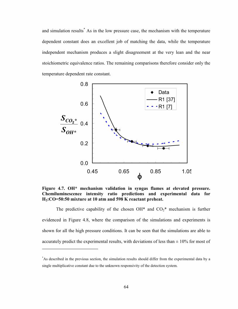
64

and simulation results* As in the low pressure case, the mechanism with the temperature

dependent constant does an excellent job of matching the data, while the temperature

independent mechanism produces a slight disagreement at the very lean and the near

stoichiometric equivalence ratios. The remaining comparisons therefore consider only the

temperature dependent rate constant.

0.0

0.2

0.4

0.6

0.8

0.45 0.65 0.85 1.05φφφφ

Data

R1 [37]

R1 [7]

*

*

OH

CO

S

S2

Figure 4.7. OH* mechanism validation in syngas flames at elevated pressure.

Chemiluminescence intensity ratio predictions and experimental data for

H2:CO=50:50 mixture at 10 atm and 598 K reactant preheat.

The predictive capability of the chosen OH* and CO2* mechanism is further

evidenced in Figure 4.8, where the comparison of the simulations and experiments is

shown for all the high pressure conditions. It can be seen that the simulations are able to

accurately predict the experimental results, with deviations of less than ± 10% for most of

*As described in the previous section, the simulation results should differ from the experimental data by a

single multiplicative constant due to the unknown responsivity of the detection system.

65

0.0

0.2

0.4

0.6

0.8

0.45 0.65 0.85 1.05φφφφ

P10-T598

P5-T298

P5-T598

*

*

OH

CO

S

S2

0.0

0.1

0.2

0.3

0.4

0.5

0 20 40 60 80 100% H2

Data

Model

*

*

OH

CO

S

S2

Figure 4.8. CO2*/OH* chemiluminescence intensity ratios (a) in H2:CO=50:50

(10 atm) and H2:CO=33:67 (5 atm) mixtures, (b) at φφφφ=0.6 for 10 atm and 598 K preheat .

most of the cases. It should be noted however, that Cdet=32 was used for the 10 atm case,

while an ~18% higher value (Cdet=38) was used for the 5 atm results. Other than this

anomaly, the overall agreement between the simulatation results and experiments is

excellent. Another observation is that Cdet was almost 60% higher than the value obtained

at atmospheric conditions. This either implies that Cdet is a function of pressure or that

there may be a systematic error in the basic chemical mechanisms used to predict the

chemiluminescence precursors, especially in the helium mixtures employed for the high

pressure conditions. The focus on helium is because both the GRI Mech 3.0 and C1

mechanisms produce OH* and CO2* chemiluminescence predictions that are quite

similar at various pressure and preheat conditions for syngas-air flames. It is also possible

that there was a systematic change in the detection system that resulted in the apparent

discrepancy of ~18% in the value of Cdet, though this is considered less likely.

Normalized OH* and CO2* chemiluminescence signals are again considered to

further investigate the accuracy of the OH* and CO2* mechanisms. For reasons cited

earlier, OH* and CO2* chemiluminescence signals are normalized with the reactant mass

(a) (b)

66

flow rates of H2 and CO respectively. The simulation results and the experiments are

compared through the expression in Eq. 18. Results for normalized OH* and CO2*

chemiluminescence as a function of equivalence ratio are shown in Figure 4.9 for a

H2:CO=50:50 syngas mixture at 10 atm and 598 K reactant preheat. The normalized

experimental OH* and CO2* chemiluminescence signals are predicted to within 5%

(except for the richest OH* data point, which is within 8%); this can be characterized as

excellent agreement.

0

100

200

300

400

500

0.45 0.65 0.85 1.05φφφφ

Data

Model

2

*

H

OH

m

S

&

&

0

1

2

3

4

5

0.45 0.65 0.85 1.05φφφφ

Data

Model

CO

CO

m

S

&

&*2

Figure 4.9. Measured and simulatated normalized chemiluminescence for (a) OH*

and (b) CO2* for a H2:CO=50:50 syngas mixture at 10 atm and 598 K reactant

preheat.

Returning to the issue of the change in the scaling constant, Cdet, for the

chemiluminescence intensity ratios at high pressure compared to atmospheric conditions,

we can investigate it further by examining the normalized signals for OH* and CO2*. As

the high pressure experiments are conducted in the contoured burner with intensifier gain

of 200, we consider only results from the atmospheric experiments with the same burner

and gain setting, i.e., the H2:CO=50:50 mixture. COH*, (the scaling constant required to

match the normalized experimental OH* signal to the simulation) decreased 9 times from

the 1 atm (air) to high pressure (He) case, while the scaling constant for CO2* decreased

(a) (b)

67

by 5.5 times. Some of the possible explanations are: 1) the simulations with He are

overpredicting IOH* and ICO2*; 2) the overprediction is due problems with the basic

chemical mechanism at high pressure; 3) the experimental signals are attenuated due to

absorption in the flame gases at high pressure; and 4) there is a systematic change in the

detection system responsivity between the low and high pressure cases. The last option is

not likely, as the detection system, flame sizes, and collection solid angles were nearly

the same in both cases. The third option, absorption is addressed in a following section.

The second and first explanations are possible, but would require the simulations to

correctly model the equivalence ratio dependence at both low and high pressure.

0

50

100

150

200

0 20 40 60 80 100% H2

Exp. Data

Model

2

*

H

OH

m

S

&

&

..

0

1

2

3

4

5

0 20 40 60 80 100% H2

Exp. Data

Model

CO

CO

m

S

&

&*2

Figure 4.10. Measured and simulated normalized chemiluminescence at φφφφ=0.6 for (a) OH* and (b) CO2* in H2:CO syngas mixtures with 40%, 50%, 60% and 80%

Hydrogen, at 10atm and 598 K reactant preheat conditions.

Validation for different fuel compositions at high pressure is considered next.

Results for the variation of normalized chemiluminescence with hydrogen content in the

syngas mixture at the same operating conditions are given in Figure 4.10 for φ=0.6. The

OH* and CO2* simulations agree well with the experimental data, predicting them to

within 5%, except for the 40% H2 mixture, where the simulations over predict the data by

25%. The flame height for this mixture was only ~6 mm, i.e., just one burner diameter.

(a) (b)

68

Even though the measure flame speed for this mixture [72] was within 5% of the value

predicted by the C1 reaction mechanism, such a compact flame could be considerably

affected by curvature, which could result in a reduction of the chemiluminescence signals

[26,10]. However, it is interesting to observe that the CO2*/OH* chemiluminescence

ratio for this case was well predicted by the simulations (see Figure 4.8). The OH* and

CO2* signals were over-predicted by the same extent, thus not affecting the CO2*/OH*

ratio. Unfortunately, similar analysis could not be performed with the experimental data

for the H2:CO=33:67 mixture at 5 atm due to lack of reliable H2 and CO mass flowrate

data. Nevertheless, it can be concluded that the chosen OH* and CO2* mechanisms can

be considered validated at elevated pressure and preheat conditions, with the caveat that

the pressure dependence may not be adequately modeled.

4.3 Thermal OH* Contribution

The above validations assume that the only contribution to the OH* signal is due

to OH created in its electronically excited state through chemical reactions. Another

possibility is that ground state OH is collisional excited. This is denoted thermal OH*.

The relative contribution of thermally OH* to the total OH* signal is computed for the

syngas flames experimentally investigated in order to evaluate its potential for systematic

errors in the validation experiments. For all the syngas mixtures tested, the spatially

integrated (10 mm) thermal OH* is determined at two extreme equivalence ratios: φ=0.7

and 1.0, using Eq. 4 (Chapter 2). The results are shown in Table 4.1. With contributions

typically under a few tenths of a percent, and always less than two percent, it can be

concluded that the effect of thermal OH* is negligible in the syngas validation

experiments.

69


experimental syngas flames.

% Thermal OH

(Li=10mm)

Syngas Mixture

(H2/CO) and

Oxidizer

Operating

Conditions

φφφφ = 0.7 φφφφ = 1.0

95-5 (Air) 1 atm, 300 K 0.13 1.73 50-50 (Air) 1 atm, 300 K 0.3 1.28

33-67 (Air) 1 atm, 300 K 0.23 1.02

50-50 (Air) 1 atm, 500 K 0.5 1.72

50-50 (O2/He) 10 atm, 600 K 0.27 5

33-67 (O2/He) 5 atm, 300 K <0.1 0.5

33-67 (O2/He) 5 atm, 600 K 0.13 1.6

4.4 Self-Absorption of OH*Emission

If a molecule can emit light going from an excited state to a lower energy state,

then the lower state can also be excited by light at the same wavelength, which lead to

absorption. The self-absorption by ground state OH will lead to a decrease in the

observed OH* signal. The importance of self-absorption is determined for the syngas

mixtures at the different operating conditions used here. Estimates of the amount of self-

absorption are calculated with Eq. 3 (Chapter 2) at two equivalence ratios: φ=0.7 and 1.0.

A path length of 5 mm was chosen for the comparison, after which it was assumed that

[OH] concentration rapidly decreased due to entrainment with cold gases surrounding our

jet flames. Theses results are presented in Table 4.2. Self-absorption is less than a 10%

effect at most conditions, though at high pressure and preheat conditions, it can be come

more signficant. For example in the H2:CO=50:50 syngas fuel at 10 atm and 600 K,

almost 20% of the signal is absorbed for the stoichiometric case (the high flame

temperature at φ=1 leads to high OH equilibrium concentrations). At lower pressures and

lean flames, self-absorption is generally less than a few percent. Thus we conclude that

70

the large change in COH* observed at high pressures is not primarily due to self-

absorption. There is some chance that it could be due to absorption by some other

species. Similarly, there may be some absorption of the CO2* chemiluminescence by CO2

or other molecules (Chapter 2). However, it is not likely that the absorption is large, as it

would be due to a broadband absorber.

Table 4.2. Fraction of OH* signal absorbed in experimental syngas flames.

% Absorption

(Li=5mm)

Syngas Mixture

(H2/CO) and

Oxidizer

Operating

Conditions

φφφφ = 1.0 φφφφ = 0.7

95-5 (Air) 1 atm, 300 K 8.4 4 50-50 (Air) 1 atm, 300 K 6 3.6

33-67 (Air) 1 atm, 300 K 5 3

50-50 (Air) 1 atm, 500 K 7.5 5

50-50 (O2/He) 10 atm, 600 K 19 8

33-67 (O2/He) 5 atm, 300 K 7 3

33-67 (O2/He) 5 atm, 600 K 12 7

In summary for syngas fuels, mechanism for both OH* and CO2*

chemiluminescence have been validated. For CO2*, the global mechanism given in Eq.

(11) (for 375 nm detection) provides excellent results for changes in equivalence ratio (at

least for lean flames), preheat temperature and dilution. For OH*, R1 appears to be the

predominant production pathway, and the temperature dependence of the rate constant

given in [37] produces accurate results. While both the OH* and CO2* mechanisms

produced generally excellent agreement with the experiments, the scaling constant used

for matching the simulation results with experimental data changed with pressure. This is

likely due, at least in part, to inaccuracies in the basic chemical mechanisms used to

simulate the laminar flames at high pressure. Another likely source for the discrepancies

is radiative trapping (absorption) of the ultraviolet emissions by CO2 and H2O at high

71

pressures. Thermal production and self absorption of OH* are not significant in the

validation experiments.

72

CHAPTER 5

HYDROCARBON FUEL VALIDATIONS

This chapter continues from the foundation laid in the previous chapter, with a

goal of identifying the important chemiluminescence formation reactions, and appropriate

rate constants, for OH*, CO2* and now CH* in lean hydrocarbon combustion. The

validation experiments were carried out primarily in laminar flames, though swirl

combustor data for methane are presented for atmospheric conditions. First, validation

results in methane flames (Section 5.1) are presented at atmospheric pressure (Section

5.1.1) and elevated pressure (Section 5.1.2). In each section, results of OH* and CO2*

chemiluminescence mechanisms are discussed followed by validation results for the CH*

mechanisms. Possible uncertainties associated with thermal excitation for OH* and CH*

are also presented along with a discussion on self-absorption (Sections 5.1.3-5.1.5).

Finally, chemiluminescence from all three species are studied in laminar premixed,

prevaporized Jet-A flames (Section 5.2).

5.1 Methane Validation

5.1.1 Atmospheric Pressure

With the chemiluminescence mechanisms validated for H2-CO fuels in the

previous chapter, the next step is consideration of additional mechanisms and species for

hydrocarbon combustion. This includes addition of the R3 formation reaction

(CH+O2→OH*+CH, Table 2.1) to the OH* mechanism, and a study of the CH*

chemiluminescence mechanisms (Table 2.2). These studies focused on methane due to its

73

wide-spread usage and well-studied kinetics. The methane data were acquired in laminar

jet flames and a turbulent, swirl combustor. Thus, these experiments are not only a test of

the validity of the modeling for laminar flames, but to some extent their applicability to

more complex systems. Additionally, the laminar methane flame data is used for

determining the ratios of the rate constants for R1 and R3 (i.e. k1/k3), by comparing them

with the laminar syngas flame data.

5.1.1.1 CO2* and OH* Chemiluminescence

The sensitivity of the simulation results to the integration length is illustrated in

Figure 5.1 for a φ = 0.8 methane-air flame. For this comparison, the simulation employed

the R1 OH* formation reaction with the rate constant from [37] (the step validated in the

previous section) and R3 with the rate constant from [45]. As before, the spatially

integrated heat release rate, and OH* and CO2* intensities are shown as a function of

spatial integration length (top axis) through the 1-d flame. The corresponding flow times

are shown on the bottom axis. The origin for the integration is, as before, the start of the

reaction zone. In addition, the values were normalized by the integrated value achieved at

33 mm (14 ms).

While the heat release begins first, the integrated OH* chemiluminescence rises

more rapidly, suggesting that most of the OH* chemiluminescence occurs within the

primary reaction zone. It plateaus quickly, within ~1 ms or 2.5 mm after the start of the

reaction zone. Thus there is little change (<1%) in IOH* with longer integration distances

(or times). On a relative basis, the CO2* chemiluminescence extends farther into the post-

flame burnout zone due to the formation of CO2* via recombination of CO and O atoms

in the near-equilibrium hot products. Therefore, ICO2* increases by ~15% if the integration

74

distance (time) is increased to 12 mm (5 ms). Similar results are found for other lean

mixtures. For mixtures very close to stoichiometric, there is a more significant sensitivity

to integration distance. At φ=1, IOH* changes by 3% for Li=2.5-12 mm (t=1-5 ms), while

ICO2* increases by nearly 33%. Thus, the CO2* simulation results are somewhat

dependent on the integration choice, and it can be expected that the comparison between

the simulations and experiments may worsen near stoichiometric conditions, mainly due

to uncertainty in predicting ICO2*.

0

0.2

0.4

0.6

0.8

1

0 1 2 3 4 5Time (ms)

Normalized Values

0 0.2 0.4 0.6 0.8 1 1.2X (cm)

Q

c

i

*OHI

*2CO

I


integrated OH* and CO2* chemiluminescence signal profiles.

Li (cm)

75

For the laminar jet flames, an integration length Li=10 mm was used.* In the swirl

combustor, an integration length per se cannot be defined as the streamlines are

convoluted due to turbulence. However, the nominal residence time (tR) can be used to

determine the appropriate integration time. The light is collected from a conical region

that changes little with equivalence ratio and is nominally 52 mm in diameter at the

center plane of the combustor. As the bulk cold flow velocity in the combustor is ~5 m/s,

it can be estimated that the product gases would be moving through the combustor at

~25 m/s. This gives a residence time of ~2 ms in the combustor, which is the value used

for the validation comparisons.

As before, the chemiluminescence ratios are compared first. It should be noted

that many of the earlier studies indicated R3 as the main contributor of OH* in

hydrocarbon flames and most researchers have assigned R3 a temperature independent

rate constant except for the recent shock tube study [45], which suggested a weak

dependence at flame temperature conditions. Thus two rate constants for the CH+O2

reaction (given in Table 2.1) were considered; one of which is temperature dependent.

Results are shown for the laminar and turbulent swirl flames in Figure 5.2. The

uncertainty in the experimental data is indicated by the error bars, which represent a ±1σ

deviation in the rms of the data. .

The results for the swirl flame are shown in Figure 5.2a. The maximum

uncertainty in the chemiluminescence intensity and equivalence ratios was approximately

±12% and ±1.5%. The best match is provided by the rate constant suggested in [7], with a

*The same value used for the atmospheric syngas flames.

76

worst case deviation from the experimental data of 25%, which occurs near the lean blow

out limit of the combustor and at the near stoichiometric condition. Even the simulation

results using R3 [45] predict within 15% for most of the experimental data and are at

least as accurate again near the lean blow out limit of the combustor and the near

stoichiometric conditions. Both the simulations and experiment show a relatively small

change in the chemiluminescence ratio with stoichiometry over the range 0.7<φ<1.

0.03

0.04

0.05

0.06

0.07

0.08

0.5 0.7 0.9 1.1φφφφ

R3 [7]

R3 [45]

R1 [37] + R3 [45]

R1 [7] + R3 [7]

Data

*

*2

OH

CO

S

S

0.02

0.03

0.04

0.05

0.06

0.5 0.7 0.9 1.1φφφφ

R3 [7]

R3 [45]

R1[37]+R3 [45]

Laminar

*

*2

OH

CO

S

S

Figure 5.2. OH* model validation: chemiluminescence intensity ratio predictions in

(a) swirl combustor and (b) laminar methane flames at p=1 atm and 298 K.

It is interesting to note that the temperature independent rate constant [7] for R3

alone does a remarkable job of predicting the data, even better than the rate constant

given in [45]. However, it should be noted that with the current experimental capability,

only the relative levels of the chemiluminescent species can be measured as opposed to

the absolute levels provided by the mechanisms. A best fit for the simulation using the

rate constant from [7] was obtained with Cdet=5.7 (the values for the other case [45] was

Cdet=144). The large change in Cdet from the syngas results (Cdet=20.1) suggests some

inaccuracy in the pre-exponential factors estimated in the original references. The results

also show that R3 alone would nearly suffice to model OH* emission under the current

operating conditions. According to the simulations, formation reaction R1 contributes

(a) (b)

77

6−9% of the total OH* chemiluminescence in the range of equivalence ratios studied

here. Thus, R1 should still be included.

If the rate constants for R1 and R3 from Smith et al. [7] are used, it can be seen

that the model prediction closely follows the other mechanisms. However in that case, R1

contributes significantly, about 44−50% of the total OH* signal. In the hot product

exhaust, where the CH radicals are essentially absent, the OH* signal is produced via the

recombination of O and H (R1), but the experimentally observed emission is very weak

there compared to that produced from CH in the reaction zone. Thus, the R1 and R3 rate

constants from Smith et al. [7] can be considered invalid even though the overall model

predictions for the signal ratio differ little from the other mechanisms.

The chemiluminescence intensity ratios from the atmospheric laminar methane

flames are shown in Figure 5.2b. The same rate constants considered for the turbulent

flames are again employed here, except for the Smith et al. [7] values. The model

predictions are again similar; for φ>0.6, all the mechanisms predict the data within 5-

10%. For φ<0.8, the predictions from the two mechanisms using R1 [37] and R3 [45]

estimated from the shock tube studies consistently deviate by 10−15% from the

predictions using the temperature independent R3 [7] alone. This latter mechanism

produces excellent agreement with the data over the whole range except at φ=0.6, where

the predictions are higher than the experimental data by 25%. For the other mechanisms,

the deviation from the experiments is ~45% at φ=0.6. Therefore, considering the results

from the swirl and laminar flames, a temperature independent R3 rate constant combined

with the R1 mechanism from the syngas validation appears to be a good choice for

modeling OH* in hydrocarbon fuel combustion.

78

This conclusion is tested by normalizing the chemiluminescence signals with the

mass flow rate of fuel (Eq. 19) and comparing to the predictions for two mechanisms:

1) R3 alone with a temperature independent rate constant, and 2) R3 with a temperature

dependent rate constant [45] and combined with the validated R1 mechanism [37].

*

***

1

2 OHLu

f

a

OH

f

OH

f

EOH IS

mm

L

C

m

S

m

tS

ρ

+≈=

∆ &

&

&

&

& (19)

The results for both the laminar and swirl methane flames are displayed in Figure

5.3a. As noted above, the integration distance/time should not have a large influence on

the results of the comparisons. The normalized OH* signals obtained from the laminar

flames are scaled by a single multiplicative constant to account for experimental

differences in order to match the swirl data. As seen in Figure 5.3a, both mechanisms are

able to simulate the measured normalized OH* signals within the experimental scatter.

However, at the leaner equivalence ratios, both mechanisms consistently under-predict

the experimental data, thus causing the higher chemiluminescence ratios seen in Figure

5.2. Nevertheless, the simulations are in excellent agreement with the experiments. This

makes it difficult to identify the correct temperature dependence for R3.

The normalized results for CO2* emission in both the atmospheric laminar and

swirl methane burners are displayed in Figure 5.3b. As with the OH* data, the laminar

flame CO2* data are scaled by a single multiplicative constant to match the swirl

combustor results. The CO2* predictions, like the OH* predictions, are within the

experimental uncertainty over most of the φ range. As the CO2* emission is more

sensitive than OH* emission to the integration distance/time, there can be a noticeable

79

0

5

10

15

20

25

30

0.5 0.7 0.9 1.1φφφφ

0

10

20

30

40

50

60

R3 [7]

R1 [37] + R3 [45]

Swirl

Laminar

f

OH

m

S

&

&*

fm

q

&

& ′′

0

0.4

0.8

1.2

1.6

2

0.5 0.7 0.9 1.1φφφφ

0

10

20

30

40

50

60

Model (2 ms)

Swirl

Laminar

Model (Li=10mm)f

CO

m

S

&

&*2

fm

q

&

& ′′


chemiluminescence for a) OH* emission and b) CO2* emission in methane flames.

change due to this parameter. The difference between the two can be clearly observed in

the simulation results for the near stoichiometric conditions in Figure 5.3b. At this

condition, the simulations with the reduced integration (2 ms) fall below the longer

(10 mm ≈ 4 ms) simulations by about 12%. Still, we can conclude that the

chemiluminescence mechanisms identified here are reasonably accurate and can be used

with appropriate chemical kinetic mechanisms to analyze the chemiluminescence signals

from CO2* and OH

* in flames with H2/CO/CH4 fuels, and possibly with other simple

hydrocarbons (at least for the atmospheric conditions tested up to this point in the thesis).

It is also interesting to note the variation in normalized chemiluminescence signal

with changes in equivalence ratio. Over the range investigated, the normalized OH*

signal increases nearly linearly with φ, while the CO2* signal appears to have a higher

(power law) dependence. Figure 5.3 also shows the normalized heat release rate

determined from the simulations; as expected, it is almost independent of equivalence

ratio for lean mixtures. Thus it can be concluded that while the OH* and CO2* signals are

correlated to the flame’s heat release, the relationship varies with equivalence ratio.

(a) (b)

80

Finally, the agreement between the swirl combustor data and the laminar results

(data and simulations) is quite remarkable. Clearly the swirl combustor is turbulent. As

noted in Chapter 3, the turbulent combustion can be characterized as either corrugated

flamelets or thin reaction zones. Thus the similarity between the laminar and turbulent

results suggests the turbulence effects on the flame, at least in this case, do not strongly

alter the dependence of the chemiluminescence on equivalence ratio.

5.1.1.2 Relationship between the rate constants of R1 and R3

At this juncture, it is appropriate to further explore the laminar methane and

syngas data to establish a relationship between the rate constants of R1 and R3. For this

comparison to be meaningful, the OH* signals (for both syngas and methane flames)

were acquired with an identical intensifier gain setting of 200. Modifying Eq. (19), we

find

hgkfkCIS

mm

L

C

m

S

m

tS ff ll

OHOHLu

f

a

OH

f

OH

f

EOH

β+≈

ρ

+≈=

∆∫∫0

3

0

12**

***

1&

&

&

&

& (20)

where f and g are functions of species concentrations related to R1 and R3 chemistry and

h is a function of experimental factors such as solid angle, detector settings, flame speed,

fuel-air ratio etc. In general, k1 and k3 are functions of temperature and hence vary along

the flame axis. The idea is that if the model predictions are correct, the multiplicative

constant COH* should be the same in scaling both syngas and methane simulations in

order to match the experimental data, for a given factor β. This would indirectly give the

relative scaling between the rate constants for R1 and R3. In syngas flames, g = 0, as

OH* is [CH] is essentially zero, and COH* can be estimated. Using the same COH* to

81

match the methane experimental data should yield β, and k3β can be considered as the

new rate constant for R3.

With the rate constant for R1 [37] and R3 [45] in Eq. (20) and matching the

experimental data yields β~0.36. So, k3 [45] has to be reduced to k3β to match the

experimental data. This establishes the relative scaling of the rate constants of R1 and R3.

or in other words, the ratio k1/k3 is determined. Similarly, if the temperature independent

rate constant for R1 [7] was used in Eq. (20), then β would be ~ 4.7, i.e., in this case k3

[7] has to be increased to match the experimental data. Here, a constant k1/k3~43 is

obtained. If a temperature range 1500-1800 K is considered, where most of the OH* is

produced (for all the lean fuel-air mixtures), and the new value for k3 used, the ratio k1/k3

varies over ~37-47 for rate constants k1[37] and k3[45]. Interestingly, this ratio is 43 if the

temperature independent rate constants were considered. This ratio k1/k3 can be

considered universal and can be used in other hydrocarbon fired combustors for

estimating OH* chemiluminescence.

At this point, it would be interesting to consider the range of values taken by k1

and k3, and based on the above analysis try to determine this range of values more

accurately. A temperature of 1800 K shall be considered without loss of generality. In the

literature k1 varies from 3.36×1013

to 8.62×1013

cm6/mol

2/s (a factor of 3) at 1800 K and

is known with better accuracy than k3, whose predicted value changes by at least two

orders of magnitude at the same temperature. So, assuming k1/k3 ~ 47, and k1 to be in the

above range of values, k3 is estimated to be in the range 7.15×1011−1.83×10

12 cm

3/mol/s

at 1800 K.

82

Based on the above analysis, both temperature dependent and independent rate

constants for R1 and R3 can be assigned as given in Table 5.1. The temperature

dependent rates were derived from Petersen et al, [37,45] and this mechanism is denoted

the Petersen-hybrid from now on. Similarly the temperature independent rates were

derived from Smith et al. [7] and shall be identified as the Smith-hybrid in the thesis.

Both these derived mechanisms excellently predict OH* chemiluminescence in

atmospheric methane-air flames. These derived mechanisms shall be further investigated

when validating experimental data at elevated pressure and preheat conditions.

Table 5.1. Suggested OH* formation reactions and their rates. Rate coefficients are

expressed as k=ATbexp(-Ea/RT) with Ea in units of cal mol

-1 and AT

b in cm

3mol

-1s-1

for two body reactions or cm6mol

-2s-1 for three body reactions (with T in K units).

# Reaction A b Ea Ref.

R1 H + O + M ↔ OH* + M 6 × 1014 0.0 6940 Petersen Hybrid

3.63 × 1013 0.0 0.0 Smith Hybrid

R3 CH + O2 ↔ OH* + CO 1.17 × 1014

-0.4 4150 Petersen Hybrid

8.47 × 1011

0.0 0.0 Smith Hybrid

5.1.1.3 CH* Chemiluminescence

Methane flames provide a good opportunity for validating CH*

chemiluminescence mechanisms for hydrocarbon systems, primarily due to the

availability of a well-validated combustion mechanism for methane. In this section, the

reported chemiluminescence mechanisms for CH* are examined and validated with

experimental data.

In this study, four mechanisms proposed in the literature (designated by the last

author of the reference source) were used to model CH* in methane flames. Each is based

on two of the formation reactions (R5-R7); the reaction rate parameters associated with

83

each are listed in Table 2.2. Of the four proposed CH* mechanisms considered, three

(Peeters [64], Carl [66] and Smith [40) are based on formation steps R6 and R7. The

Peeters mechanism has temperature independent rate constants, while the Carl

mechanism is an updated version that adds temperature dependence to both formation

rates but matches the large rate constant ratio, k2/k3~500, of Peeters at ~650 K. However,

it should be noted that k2/k3 in the Peeters mechanism is a constant, while in the Carl

mechanism the ratio varies from 420 at 700 K to 15 at 2000 K. The Smith mechanism

includes temperature dependence only for the O2 step, and has a much lower k2/k3 value

decreasing from 25 to 12 for the same 700-2000 K range. On the other hand, the fourth

mechanism (Petersen [64]) uses R5 and R6. To use R5 with the GRI mechanism requires

the addition of reactions for the production and destruction of C2, as outlined in the same

reference.

As with OH* and CO2* chemiluminescence, CH* chemiluminescence was

acquired both in atmospheric-pressure laminar and swirl burners. Earlier, a residence

time of ~2 ms was established for comparisons to the swirl burner, while an integration

length of 10 mm was used for the laminar flame case. For comparing simulated CH*

chemiluminescence to the data, however, it is sufficient to use one integration length

(10 mm ≈ 4 ms) in both burners. This is due to the fact that CH* is formed only in the

narrow region where C2H or C2 is present, i.e., in the primary reaction zone for the lean

methane-air flames.

As before, we start by examining chemiluminescence signal ratios. As the OH*

chemiluminescence is almost completely associated with the primary reaction, like CH*,

it as chosen for the ratio comparison. Also as the OH* chemiluminescence mechanism

84

(Table 5.1) was validated above, the CH*/OH* ratio comparison should directly reveal

the accuracy of the CH* mechanisms considered. The measured chemiluminescence

signal ratio is related to the simulated value through the expression below.

*

*det

*

*

OH

CH

OH

CH

I

IC

S

S= (21)

0

0.1

0.2

0.3

0.4

0.5

0.5 0.7 0.9 1.1φφφφ

Swirl

Carl

Smith

Peeters

Petersen

Laminar

*

*

OH

CH

S

S

0

2

4

6

0.5 0.7 0.9 1.1φφφφ

Swirl

Carl

Peeters

Laminar

f

CH

m

S

&

&*

Figure 5.4. Comparison between experimental results and model predictions for a)

CH*/OH* chemiluminescence intensity ratio and b) normalized CH* emission in

methane flames at 1 atm and 298 K.

Results for the CH*/OH* chemiluminescene ratio are shown for the swirl burner

and laminar jet flames in Figure 5.4a. First, it is worth noting the excellent agreement

between the laminar and swirl flame results, except near the lean blow out limit of the

swirl combustor. The figure also includes the simulation results for the four mechanisms.

The simulation results for each were multiplied with a chosen Cdet such that the least

square difference (across the φ range) is minimized. The best agreement with the

experimental data is provided by the Peeters mechanism, which matches the laminar data

across the complete range within the experimental uncertainty, and it matches the swirl

data except near its lean blowout limit. The mechanism that includes the C2 formation

step (Petersen) provides the poorest overall match. It should be noted here that the lack of

(a) (b)

85

accurate rate kinetic information for C2 formation and destruction reactions could be a

significant cause for this disagreement. The somewhat poorer comparison produced by

the Smith mechanism argues against its lower k2/k3 ratio. The Smith mechanism

significantly over predicts the data, especially for φ<0.8. The Carl mechanism does a

reasonable job for φ>0.85, but over predicts the data for lean mixtures. Thus both the

Petersen and Smith mechanisms can be eliminated without further investigation.

The relatively good agreement between the Peeters and Carl mechanisms is

further investigated by considering the variation of normalized CH* chemiluminescence

signal with equivalence ratio as shown in Figure 5.4b. Experimental and simulated CH*

chemiluminescence signals, normalized by fuel flow rate, used for the validation can be

compared using Eq. (19) (replacing OH* with CH* values). The simulation results for

each were multiplied with a given CCH* in order to minimize the overall deviations (the

least square difference).* With this scaling, the agreement between the Peeters and Carl

mechanisms is even more pronounced, in spite of the inherent differences in the

temperature dependence of the reaction rate constants for R6 and R7.

The agreement between the Peeters and Carl mechanisms, with their different

temperature dependence for k2/k3 occurs due to a offsetting change in the concentration

ratio [O]/[O2] and k2/k3 for the Carl mechanisms in the methane flames studied. For the

Peeters mechanism, R2 dominates CH* production in the lean (atmospheric) methane

flames, and the formation of CH* is essentially given by k2,P[C2H][O]. For the Carl

*This does not provide validation of the absolute values for the reaction rate constants, since the absolute

responsivity of the detection system are not known.

86

values (k2,C and k3,C), both reactions are important; thus the ratio of the CH*

chemiluminescence for the two mechanisms scales like [ ][ ]

+

O

O

k

k

k

k

C

C

C

P 2

,2

,3

,2

,21 . Since

CP kk ,2,2 is a constant (~1.8), the two mechanisms will give the same result if k2/k3 for the

Carl mechanism varies with temperature in a similar fashion to [O2]/[O], which turns out

to be the case in our flames.

In summary, the best agreement with the experimental results is provided by the

Peeters (temperature independent) rate constants, though simulations with the Carl

(temperature dependent) rate constants are nearly as good. Overall, the results suggest

that either the Carl or Peeters mechanisms could be used to predict CH*

chemiluminescence in atmospheric methane-air flames.

5.1.2 Elevated Pressure

Experimental measurements of flame chemiluminescence at elevated pressure can

help in evaluating the robustness of the chemiluminescence mechanisms, and in the case

of OH* and CH*, may also help in differentiating the best candidates determined in the

atmospheric experiments. Therefore, data was acquired in 5 and 10 atm laminar methane

flames. OH*, CH* and CO2* chemiluminenscence was acquired at room temperature

conditions at both pressures, and with 598 K reactant preheat at 5 atm. As with the syngas

experiments, a O2:He oxidizer mixture (1:5) was used to aid in flame stabilization at high

pressure conditions. The San Diego mechanism [76], which includes helium, was used

instead of GRI Mech 3.0, to simulate the flames.

87

5.1.2.1 CO2* and OH* Chemiluminescence

As in the previous cases, the sensitivity of the simulated chemiluminescence

signals to integration length is examined first. Example results for φ=0.8 are shown in

Figure 5.5. The OH* chemiluminescence is simulated with the R1 and R3 rate constants

0.0

0.2

0.4

0.6

0.8

1.0

0 0.2 0.4 0.6 0.8 1

Li (cm)

Norm

alized Values

Q

c

i *OHI

*2CO

I


integrated OH* and CO2* chemiluminescence signal profiles in a methane flame at

10 atm and room temperature conditions. The equivalence ratio is 0.8.

given in Table 5.1, with the values normalized by the integrated value achieved at 5 cm

downstream of the reaction zone.

High pressure flames are generally characterized by extremely thin reaction

zones, and this can be clearly inferred from the heat release rate profile in Figure 5.5. The

heat release approaches a plateau value, within a few hundred micrometers after the start

of the reaction zone. The reaction zone is also thinner than that of the high pressure

syngas flame presented in the last chapter. In high pressure methane flames, the post-

88

flame product gases are a source of both OH* and CO2* chemiluminescence, due to the

formation of OH* via R1 (O+H+M) and CO2* via CO+O.

To aid in determining the integration length for the simulations, flame

chemiluminescence images were also acquired with the same ICCD camera employed in

the high pressure syngas experiments. Now, however, the intensity at any pixel is

potentially due to a combination of all three sources (OH*, CH* and CO2*). As the

product zone’s contribution to the total OH* and CO2* chemiluminescence signal

significantly increases for near stoichiometric flames, a methane flame image for a

10 atm, 298 K and φ=0.97 is shown in Figure 5.6a. The raw image shows a much more

significant contribution (to the total OH*and CO2* signals) from the hot products,

especially for regions near the flame tip. Horizontal cuts at two locations along the flame

height are shown in Figure 5.6b, one at 20% and the other at 80% of the flame height. In

each of the plots, the peaks indicate the approximate flame location. From the results

lower in the flame, the signal intensity is seen to drop to ~4% of the peak value at 2 mm

from the flame. For the higher location, the intensity drops much less rapidly, only to

~30% of the peak signal at 3.6 mm from the flame. This clearly confirms the contribution

of the hot product region to the total chemiluminescence signal particularly for near

stoichiometric flames.

It can also be inferred that an integration distance of 5 mm for the lower half of

the flame and at least 10 mm for the upper half of the flame would include most of the

exhaust regions where OH* and CO2* chemiluminescence signals are produced. For

Li=5−10 mm; IOH* changes by about 4%, while ICO2* change by nearly 6%. Still, this can

be characterized as a mild dependence on integration distance between 5 and 10 mm.

89

0.01

0.1

1

0 1 2 3 4 5

X (mm)

~ 0.8h

Products

0.01

0.1

1

0 1 2 3 4 5

r (mm)

~ 0.2h

ProductsNorm

alized Intensity

(a) (b)

Figure 5.6. Chemiluminescence image analysis for a methane flame at 10 atm, 298 K

and φφφφ=0.97. (a) Raw image (burner diameter is 6 mm) and b) radial (line of sight) Intensity profiles from the burner center axis, at 20% and 80% of the flame height.

Similar results are found for other lean mixtures and for the flames at 5 atm. For near

stoichiometric mixtures, a greater fraction of the chemiluminescence is produced in the

high temperature product gases, similar to that observed in atmospheric conditions. At

φ=1, and at identical operating conditions, IOH* changes by about 8% for Li ranging from

5−10 mm, while ICO2* increases by about 9%. Since the lean cases showed little

sensitivity to the choice of integration length, an Li of 10 mm was chosen for the high

pressure validations.

For the comparisons to the high pressure data, OH* chemiluminescence was

modeled with two mechanisms, both include R1 and R3. The mechanisms are given in

Table 5.3 and the difference lies in whether both R1 and R3 have temperature

90

independent rate constants (Smith hybrid) or temperature dependent rate constants

(Petersen hybrid). Again, only one mechanism for CO2* is considered.

0

0.02

0.04

0.06

0.08

0.1

0.5 0.7 0.9 1.1φφφφ

Data

Petersen Hybrid

Smith Hybrid

*

*

OH

CO

S

S2

Figure 5.7. OH* model validation in methane flames at elevated pressure

conditions: chemiluminescence intensity ratio predictions for flames at p=10 atm

and 298 K.

Results for the CO2*/OH* chemiluminescence ratio in a methane flame at 10 atm

and 298 K are shown in Figure 5.7. The two simulation results are multiplied by values of

Cdet such that they match for a stoichiometric mixture. It can be seen that none of the

mechanisms seem to predict the equivalence ratio variation of the CO2*/OH*

chemiluminescence intensity ratio. The experiments depict almost a monotonic decrease

while the models predict a non-monotonic variation of the CO2*/OH* ratio. While the

results point out to the possibility of errors in the OH* or CO2* mechanisms, the

chemiluminescence signals have to be considered separately to determine where the

problem lies. For this reason, the OH* and CO2* chemiluminescence signals were

normalized with the fuel mass flow rate, and the results are shown in Figure 5.8.

91

0

3

6

9

12

15

0.5 0.7 0.9 1.1φφφφ

Data

Petersen Hybrid

Smith Hybrid

f

OH

m

S

&

&*

0.0

0.2

0.4

0.6

0.8

1.0

0.5 0.7 0.9 1.1φφφφ

Data

Model

f

CO

m

S

&

&*2

Figure 5.8. OH* mechanism validation in methane flames at elevated pressure

conditions: (a) normalized OH* emission and (b) CO2* emission for flames at

10 atm and 300 K reactants.

First, it can be seen that both OH* mechanisms are less accurate at these

conditions but the Petersen hybrid mechanism provides better predictions than the Smith

hybrid, likely due to the temperature dependent rates it employs for R1 and R3. On the

other hand there is excellent agreement between the simulations and the experiments for

the CO2* chemiluminescence. So, it is most likely the inability of the OH* mechanism to

predict OH* chemiluminescence accurately that caused the discrepancy in the CO2*/OH*

chemiluminescence intensity ratio results as presented in Figure 5.7. The measured OH*

variation with φ is more dramatic than predicted by either mechanism.

Comparisons for the simulations (with the Petersen hybrid OH* mechanism) with

all the methane experimental data obtained at high pressure are shown in Figure 5.9

(CO2*/OH* ratio) and Figure 5.10 (normalized signals). For the ratios, a value of 10 was

used for the scaling constant Cdet. The simulated ratios are in poor agreement with the

experimental data; not only do they have the wrong trend with φ, they do not display the

correct pressure dependence. The experiments indicate a negligible effect of pressure and

(a) (b)

92

0

0.02

0.04

0.06

0.08

0.1

0.5 0.7 0.9 1.1φφφφ

P5-T298

P5-T598

P10-T298

*

*

OH

CO

S

S2

Figure 5.9. CO2*/OH* chemiluminescence intensity ratios in methane flames at

elevated pressure. Experimental data represented by symbols and simulation results

depicted by lines: dashed line for 5 atm-298 K cases, dot dashed line for 5 atm-598 K

case and solid line for 10 atm-298 K case.

preheat on the CO2*/OH* chemiluminescence intensity ratio at these conditions.

Results for the normalized OH* and CO2* chemiluminescence signals are shown

in Figure 5.10. The OH* and CO2* simulations were scaled by single values for COH* and

CCO2*, chosen to match the 10 atm-298 K experimental data. Both the OH* and CO2*

simulation results deviate significantly from the experimental behavior. While the trend

with φ is qualitatively correct, both the OH* and CO2* simulations fail to capture the

pressure or preheat dependence. The OH* mechanism fails most for the preheated case,

where the predictions are off by ~100%. On the other hand, the CO2* mechanism shows

little pressure dependence, unlike the experiments. It is interesting to note that reactant

preheat has little effect on the measured OH* and CO2* chemiluminescence at 5 atm.

93

0

4

8

12

16

20

0.5 0.7 0.9 1.1φφφφ

P5-T298

P5-T598

P10-T298

f

OH

m

S

&

&*

0.0

0.2

0.4

0.6

0.8

1.0

0.5 0.7 0.9 1.1φφφφ

P5-T298

P5-T598

P10-T298

f

CO

m

S

&

&*2

Figure 5.10. Normalized chemiluminescence signals in methane flames at elevated

pressure: (a) OH* emission and (b) CO2* emission. Experimental data represented

by symbols and model predictions depicted by lines: dashed line for 5 atm-298 K

cases, dot dashed line for 5 atm-598 K case and solid line for 10 atm-298 K case.

This discrepancy between the simulations and experimental data may be due to

several causes. In the case of OH* for the room temperature conditions, the increase in

OH* signal near stoichiometric conditions may be due to thermally produced OH*. Self-

absorption of OH* by ground state OH molecules may become important at high pressure

conditions and this aspect shall be further discussed in Section 5.5. As mentioned in

Chapter 2, the ultraviolet OH* emission can also be absorbed by other molecules such as

CO2 and H2O at high pressures. For the preheated case, the San Diego mechanism also

consistently over predicts flame speeds by over 20% as compared to the experiments. So,

there is a possibility that the mechanism might be over predicting the precursor species

for OH* formation such as O, H, O2 and CH, and this would directly impact the

integrated chemiluminescence intensities. Also as significant fractions of both OH* and

CO2* are produced in the exhaust zone at high pressure according to the models, any

difference in experimental conditions in the product gas zone such as product gas cooling

(a) (b)

94

0.4

0.6

0.8

1

1.2

300 350 400 450 500 550

λλλλ(nm)

CO

2* Background, A.U

P1-T298

P5-T298

P5-T598

P10-T298

P=1 atm

Figure 5.11. Spectral shape of the CO2* continuum in methane flames at various

pressure conditions at φφφφ~075.

by N2 entrainment could severly effect the measured OH* and CO2* signals. Moreover,

the results for CO2* could also be explained if absorption of the CO2* signal by the

ground state was signficant. It is also possible that the CO2* signal at 375 nm might be

corrupted by other emitters such as HCO or water [57-59].

This can be partially verified by considering the “continuum” near the vicinity of

375 nm for the experiments considered. The “CO2* background” for an equivalence ratio

of 0.8 is considered for all the pressure conditions, and the results for scaled “CO2*

background” is shown in Figure 5.11. The spectral shape of the continuum at elevated

pressure conditions is different than at atmospheric pressure. Moreover, there are clear,

distinct peaks in the spectra near the vicinity of 375 nm, for all operating conditions

which might suggest that other emitters are superimposed on the continuum.

95

It is also worth investigating the basic reaction mechanism (San Diego [76]) for

methane combustion used here. The normalized OH* and CO2* signals predicted by the

San Diego mechanism are compared to those from GRI Mech 3.0 in Figure 5.12. GRI

Mech 3.0 always predicts a higher OH* chemiluminescence signal than the San Diego

mechanism. Additionally, the OH* signals predicted by the mechanisms do not have the

same pressure or preheat temperature dependence. For example at 1 atm, OH* signal

predicted by San Diego mechanism has to be multiplied by ~2.2 to match the GRI Mech

results while this multiplicative constant changes to ~1.5 at 5 and 10 atm. So, it is

possible that a similar phenomenon is explains the high pressure methane-O2/He flames

used here. In case of normalized CO2* signal, the mechanisms produce excellent

agreement at high pressure conditions but they differ significantly at atmospheric

conditions. This suggests that both mechanisms predict the same CO and O profiles, but

differ in their CH and H profiles.

0

5

10

15

20

25

0.5 0.7 0.9 1.1φφφφ

P1-T298

P5-T598

P10-T298

f

OH

m

S

&

&*

0

0.4

0.8

1.2

1.6

2

0.5 0.7 0.9 1.1φφφφ

P1-T298

P5-T598

P10-T298

f

CO

m

S

&

&*2

(a) (b)

Figure 5.12. OH* and CO2* model predictions with San Diego (lines) and GRI Mech

3.0 (lines with symbols) reaction mechanisms in methane air flames at various

pressure and temperature conditions.

So, in conclusion, the Petersen hybrid mechanism can be used to qualitatively

predict OH* chemiluminescence in methane flames at high pressure and preheat

96

conditions. The CO2* mechanism is not able to predict the intensity at 375 nm, possibly

due to interferences (emission and absorption) from other species. Also further

investigation into the production and destruction of CO2* at various operating conditions

may be required. However, both OH* and CO2* mechanisms can be used to reasonably

predict the chemiluminescence signals’ equivalence ratio variation.

5.1.2.2 CH* Chemiluminescence

As CH* chemiluminescene occurs only in the reaction zone, any integration

length (Li) that exceeds the reaction zone thickness should be sufficient for modeling

purposes. So, an integrated length Li=10 mm was used as with the case of CO2* and OH*

chemiluminescence models. The CH*/OH* ratios at 10 atm and 298 K are shown in

Figure 5.13a. The simulations use the Petersen hybrid mechanism for OH*, and the

Peeters and Carl mechanisms for CH*. The Carl mechanism appears to better predict the

0.0

0.1

0.2

0.3

0.4

0.5

0.5 0.7 0.9 1.1φφφφ

Data

Peeters

Carl

*

*

OH

CH

S

S

0.0

0.2

0.4

0.6

0.8

1.0

0.5 0.7 0.9 1.1φφφφ

Data

Peeters

Carl

f

CH

m

S

&

&*

Figure 5.13. Comparison between experimental results and simulations for (a)

CH*/OH* chemiluminescence intensity ratio and (b) normalized CH* emission in

methane flames at 10 atm and 298 K.

(a) (b)

97

experiments compared to the Peeters mechanism. However, the failure of the OH*

mechanism makes the comparison problematic. So the variation of normalized CH*

chemiluminescence is considered to further investigate the CH* mechanisms.

The normalized signals are shown in Figure 5.13b; the CCH* for both simulations

were chosen based on a least-square error fit. Both the Carl and Peeters mechanisms

predict the experiments with excellent accuracy, within the experimental uncertainty,

despite their inherent differences in the temperature dependence of reactions R6 and R7.

The deviation of the models from the experiments is at most ~15%. Still, the Carl

mechanism slightly outperforms the Peeters mechanism, which over predicts the

equivalence ratio dependence. So, the Carl mechanism is used further to examine CH*

chemiluminescence in methane flames.

0.0

0.2

0.4

0.6

0.8

1.0

1.2

0.5 0.7 0.9 1.1φφφφ

P5-T298

P5-T598

P10-T298

*

*

OH

CH

S

S

0.0

0.5

1.0

1.5

2.0

2.5

3.0

3.5

0.5 0.7 0.9 1.1φφφφ

P5-T298

P5-T598

P10-T298

f

CH

m

S

&

&*

(a) (b)

Figure 5.14. Validation of CH* chemiluminescence model in methane flames at

elevated pressure: (a) CH*/OH* intensity ratio and (b) normalized CH*

chemiluminescence signal. Experimental data represented by symbols and model

predictions depicted by lines: dashed line for 5 atm-298 K cases, dot dashed line for

5 atm-598 K case and solid line for 10 atm-298 K case.

Results for all the experimental data obtained in the high pressure methane flames

are shown in Figure 5.14, both CH*/OH* intensity ratios (Figure 5.14a) and normalized

signals (Figure 5.14b). The simulations qualitatively agree with the change in the

98

CH*/OH* dependence on φ with pressure. At 1 atm, the signal ratio was seen to increase

with φ, at high pressures this is reversed. The scaling constant CCH* for the normalized

signals is chosen to best match the experimental data at 5 atm without preheat. It can be

seen in Figure 5.14b that the variation of the normalized CH* signal with φ is in good

agreement with the experiments at 5 atm, with and without preheat. In addition, the

model correctly captures the chemiluminescence increase caused by preheating.

However, the CH* model predictions do not capture the drop in signal when the pressure

is increased to 10 atm. This disagreement between the experiments and the model

predictions can be due to several reasons. One of the important reasons could be due to

the lack of accurate quenching rate information of CH* radicals at high temperature

conditions [38]. The very small concentrations of ground state CH present in flames

eliminates the possibility of self-absorption of CH* chemiluminescence by ground state

CH radicals. Another possibility is that the San Diego mechanism has significant

uncertainty in predicting the profiles for C2H, the precursor for CH*. So, the San Diego

mechanism predictions are compared with GRI Mech 3.0 in methane-air flames at similar

pressure and temperature conditions. It can be seen in Figure 5.15 that the San Diego

mechanism over-predicts the GRI Mech estimates for the normalized CH* signal. The

CH* signals predicted by the mechanisms also do not scale well at different operating

conditions. For example at 1 atm, the scaling constant to match the CH* signal predicted

by San Diego mechanism with that of the GRI Mech 3.0 results is ~0.4. This scaling

constant changes to ~0.65 at 5 atm and ~0.85 at 10 atm. Moreover, the variation of the

CH* signal with equivalence ratio is also different for both mechanisms. At 10 atm and

room temperature conditions, GRI Mech 3.0 predicts an increase of ~7.5 while the San

99

Diego mechanism estimates an increase of ~4 in the 0.6-1 equivalence ratio range. So,

even though the reaction mechanisms match in their estimates of flame properties such as

the laminar flame speeds or ignition delays with 10-15% accuracy, they could have

significant disagreement in their estimates of flame chemiluminescence signals.

It can be concluded that given the experimental and modeling uncertainties, the

CH* mechanism is able to qualitatively predict the experimental results satisfactorily.

The CH* model predictions could be used for a particular pressure and temperature

condition but the model predictions should be scaled with caution for other operating

conditions.

0

5

10

15

20

0.5 0.7 0.9 1.1φφφφ

P1-T298

P5-T598

P10-T298

f

CH

m

S

&

&*

Figure 5.15. CH* model predictions with San Diego (lines) and GRI Mech 3.0 (lines

with symbols) reaction mechanisms in methane air flames at various pressure and

temperature conditions.

5.1.3 Thermal OH*

Thermal OH* results for the methane experiments are shown in Table 5.2. The

relative contribution of thermal OH* to the total OH* signal was calculated as before

100

using Eq. 4. Thermally excited OH* increases exponentially with temperature. So, two

equivalence ratios were considered for the analysis: φ=0.7 and 1.0. It can be seen that

thermal excitation becomes important at high pressure and temperature conditions

particularly for near stoichiometric conditions. For example, the thermal pathway can

contribute as much as quarter of the total OH* signal at 5atm and 600 K. Of course, these

calculations are very simplified based on the assumption that thermal equilibrium exists

at every point in the flame.


methane experiments.

% Thermal OH

(Li=10mm)

Methane

and Oxidizer

Operating

Conditions

φφφφ = 0.7 φφφφ = 1.0

CH4/Air 1 atm, 300 K <0.1 1

CH4 (O2/He) 5 atm, 300 K 1.3 16

CH4 (O2/He) 5 atm, 600 K 10 25

CH4 (O2/He) 10 atm, 300 K 2.7 25

5.1.4 Thermal CH*

Thermal excitation of CH is also possible, though generally negligible due to the

very low concentrations of CH radical in the flame. Thermal CH* is calculated for the

experimental methane flames using Eq. 6. The values in Table 5.3 verify this. So, for all

practical purposes the contribution from thermally excited CH in the experimentally

investigated flames is negligible.

101

Table 5.3. Thermal CH* contribution (as percentage of the total CH* signal) in

methane experiments.

% Thermal CH

(Li=10mm)

Methane

and Oxidizer

Operating

Conditions

φφφφ = 0.7 φφφφ = 1.0

CH4/Air 1 atm, 300 K 0.006 0.054

CH4 (O2/He) 5 atm, 300 K 0.001 0.018

CH4 (O2/He) 5 atm, 600 K 0.004 0.034

CH4 (O2/He) 10 atm, 300 K 0.001 0.025

5.1.5 Self-Absorption

Estimates of self-absorption are calculated for all the methane flames that were

experimentally investigated. Self-absorption was computed in the same manner described

in Chapters 2 and 4. While it was estimated to be at most a ~10-15% effect in the high

pressure syngas flames, it can be seen in thus absorption changes with flame location. For

example, there is difference in self absorption from the side facing the detector and from

the rear of the flame, as the path lengths and spatial distribution of the OH* radicals are

different. However, this computation gives order of magnitude estimates that can be

compared across different conditions.

Table 5.4 that OH* self absorption is more significant in the high pressure methane

flames, especially near stoichiometric conditions. It can also be observed that the

reduction in OH* signal by absorption increases with the integration length (residence

time). Moreover, it can be seen that absorption is a function of pressure, temperature and

equivalence ratio. This has immediate implications for the scaling constant (COH*).

According to the results in the table, the scaling constant can change as much as 2 times

across the equivalence ratio range. However, this change was not observed in the

102

experiments. It should be noted that this calculation is a worse case estimate, as it uses a

peak absorption coefficient. Also the actual flame is axisymmetric rather than 1-d, and

thus absorption changes with flame location. For example, there is difference in self

absorption from the side facing the detector and from the rear of the flame, as the path

lengths and spatial distribution of the OH* radicals are different. However, this

computation gives order of magnitude estimates that can be compared across different

conditions.

Table 5.4. Fraction of OH* signal absorbed in methane experiments.

Methane

and Oxidizer

Operating

Conditions

% Absorption

(Li=10 mm)

% Absorption

(Li=5mm)

φφφφ = 1.0 φφφφ = 0.7 φφφφ = 1.0 φφφφ = 0.7

CH4/Air 1 atm, 300 K 5 3 5 2

CH4 (O2/He) 5 atm, 300 K 30 13 20 8

CH4 (O2/He) 5 atm, 600 K 41 31 21 14

CH4 (O2/He) 10 atm, 300 K 39 20 24 9

5.2 Jet-A Validation

5.2.1 Atmospheric Pressure

Jet-A is a primary fuel in aeropropulsion applications, and as a light oil fuel is

relevant in many other combustion applications. In spite of its importance, there have

been very few studies that investigated flame chemiluminescence applications in Jet-A

systems. The preliminary results presented in this thesis represents an effort to validate

CH* and OH* chemiluminescence mechanisms in this complex fuel.

103

5.2.1.1 CO2* Chemiluminescence

Jet-A is a complex, multi-component heavy hydrocarbon fuel that has a widely

varying composition. The apparent underlying “blue continuum” observed in H2-CO

flame spectra in the wavelength range 200-700 nm is primarily due to CO2*

chemiluminescence while there are claims of contribution from other sources such as

H2O2, H2O etc. though negligibly. However, in the combustion of complex hydrocarbon

fuel such as Jet-A, there may be other sources (such as HCO) which might corrupt this

“CO2* background” and the model for CO2* chemiluminescence would no longer be

valid.

0.4

0.6

0.8

1

1.2

1.4

1.6

300 350 400 450 500 550

λλλλ(nm)

CO

2* Background, A.U

H2:CO = 50:50

CH4

Jet-A

Figure 5.16. Nominal “CO2* background” spectral shape in typical premixed flames

of syngas mixtures, methane and Jet-A fuels at atmospheric pressure conditions.

To appreciate this issue, the spectral shape of the “CO2* background” in a typical

syngas mixture (H2:CO=50:50), methane and Jet-A flame are compared in Figure 5.16.

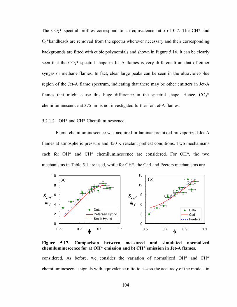
104

The CO2* spectral profiles correspond to an equivalence ratio of 0.7. The CH* and

C2*bandheads are removed from the spectra wherever necessary and their corresponding

backgrounds are fitted with cubic polynomials and shown in Figure 5.16. It can be clearly

seen that the CO2* spectral shape in Jet-A flames is very different from that of either

syngas or methane flames. In fact, clear large peaks can be seen in the ultraviolet-blue

region of the Jet-A flame spectrum, indicating that there may be other emitters in Jet-A

flames that might cause this huge difference in the spectral shape. Hence, CO2*

chemiluminescence at 375 nm is not investigated further for Jet-A flames.

5.2.1.2 OH* and CH* Chemiluminescence

Flame chemiluminescence was acquired in laminar premixed prevaporized Jet-A

flames at atmospheric pressure and 450 K reactant preheat conditions. Two mechanisms

each for OH* and CH* chemiluminescence are considered. For OH*, the two

mechanisms in Table 5.1 are used, while for CH*, the Carl and Peeters mechanisms are

0

2

4

6

8

10

0.5 0.7 0.9 1.1φφφφ

Data

Petersen Hybrid

Smith Hybrid

f

OH

m

S

&

&*

0

3

6

9

12

15

0.5 0.7 0.9 1.1φφφφ

Data

Carl

Peeters

f

CH

m

S

&

&*


chemiluminescence for a) OH* emission and b) CH* emission in Jet-A flames.

considered. As before, we consider the variation of normalized OH* and CH*

chemiluminescence signals with equivalence ratio to assess the accuracy of the models in

(a) (b)

105

Jet-A flames. Results for normalized OH* and CH* emission signals are given in Figure

5.17, and they are compared with simulations using Eq. 19 and Eq. 21.

It can be seen in Figure 5.17a that the OH* chemiluminescence model predictions

show significant deviation in the leaner equivalence ratio regime. However, the Smith

hybrid performs marginally better than the Petersen hybrid in this region. So, the OH*

mechanisms should be used with caution for predictions in lean equivalence ratios but

they can give excellent estimates for the near stoichiometric mixtures. The discrepancy

found in the lean equivalence ratios could be due to the inaccurate estimates of the OH*

precursors (such as O, H, CH and O2) by the Jet-A reduced mechanism itself. It is also

possible that there is another OH* formation mechanism that is not accounted in the

present analysis. Finally, lack of information about the collisional quenchers in this flame

and their quenching rates could be the cause.

The CH* chemiluminescence results are shown in Figure 5.17b; both the Peeters

and Carl mechanisms produce very good agreement with the experimental data, as in the

methane validations. The two mechanisms provide essentially identical results, except

below φ~0.7, where the Peeters mechanism appears to provide a better match. However,

the difference between the two is not large, and possible errors in the reduced mechanism

preclude identifying an optimum mechanism. However, it is interesting to note that the

simulations indicate that for near stoichiometric conditions, R2 and R3 contribute almost

equally to the CH* signal in the Carl mechanism, while R2 dominates R3 for the Peeters

mechanism. In spite of these differences, it is remarkable to find excellent agreement

between the two. In summary, preliminary experimental results indicate that the CH*

chemiluminescence can be predicted with models employing formation reactions R6 and

106

R7, as in methane flames. Furthermore, it is interesting to note that despite the significant

variation in k2/k3 for the two mechanisms, they again provide similar results at

atmospheric pressure. However, more experiments have to be performed at various

pressure and preheat conditions to test the robustness of the Jet-A combustion mechanism

as well as the OH* and CH* chemiluminescence mechanisms.

0

0.5

1

1.5

2

2.5

0.5 0.7 0.9 1.1φφφφ

Data

Model

*

*

OH

CH

S

S

Figure 5.18. CH*/OH* chemiluminescence intensity ratio variation with equivalence

ratio in a premixed, prevaporized and preheated (450K) Jet-A flame at 1 atm.

The CH*/OH* chemiluminescence signal ratios are considered next for the sake

of completeness. The measured chemiluminescence signal ratio is related to the simulated

ratio through the expression given in Eq. 21. OH* chemiluminescence is modeled with

the Smith hybrid mechanism, and CH* chemiluminescence is modeled with the Peeters

mechanism. The experimental and simulated CH*/OH* ratios are shown in Figure 5.18.

It can be noticed that the simulations produce good agreement at the near stoichiometric

conditions but start deviating from the experimental data in the leaner equivalence ratios.

107

This can be explained based on the results in Figure 5.17. OH* is significantly

underestimated in the lean regime while CH* is predicted excellently throughout the

equivalence ratio range. Hence, the steep increase found in the simulated ratios in the

leaner equivalence ratios.

In summary, mechanisms for OH*, CO2* and CH* chemiluminescence have been

validated in two hydrocarbon fuels. The CO2* global mechanism validated in the syngas

tests provides an excellent match to the atmospheric methane data. However, in high

pressure methane flames and Jet-A flames there is significant interference from other

emission sources. The validated OH* mechanism adds one more formation step (R3) to

the mechanism validated in Chapter 4. The temperature dependence given in [45] for k3

provided the best results. In addition, the ratio k1/k3 was estimated by comparing the

syngas and methane atmospheric data. As the literature shows a reasonable agreement on

the magnitude for k1, this ratio was used to provide an improved estimate for the pre-

exponential factor (i.e., the A coefficient) for k3. The validated OH* mechanism captures

the φ and pressure dependence well, but failed to capture the reactant preheat effect at

high pressure. A mechanism for CH* was also validated, though two sets of rate

constants (Carl and Peeters) were able to predict the methane and Jet-A experimental

data. The Peeters rate constants produced a better match for the φ dependence in the

atmospheric flames, while the Carl values provided slightly better φ and preheat

temperature dependence results at elevated pressure. As in the syngas case, there are

possible systematic errors in the high pressure simulations due to inaccuracies in the

flame reaction mechanisms employed here. In addition, radiative trapping and thermal

OH* production are likely error sources for the high pressure experiments. Excellent

108

agreement between the global chemiluminescence measurements in the laminar and swirl

methane flames was observed. The fact that the swirl combustor conditions are likely in

the corrugated flamelet or thin reaction zone regimes suggests that the dependence of

chemiluminescence on conditions in laminar flames have relevance in a number of

turbulent flames.

109

CHAPTER 6

IMPLICATIONS FOR COMBUSTION SENSING

The goal of this chapter is to examine chemiluminescence using the mechanisms

for OH*, CO2* and CH* validated in the previous chapters. Specifically, the effect of

pressure, reactant preheat, aerodynamic strain rate, fuel-air ratio and product recirculation

on chemiluminescence signals are examined for lean premixed methane and syngas

flames. The fundamental aspects of OH*, CH* and CO2* chemiluminescence in

premixed flames are investigated in the first section. The usefulness of flame

chemiluminescence for sensing important combustion parameters, specifically heat

release rate and reaction zone equivalence ratio, are examined next. As part of the heat

release studies, the CO2* background is estimated at the OH* and CH* detection

wavelengths and its implications are presented. This is followed by a discussion on the

relative contributions of thermal and chemical sources to OH* in the final section. While

the findings presented in this chapter are based on laminar data and simulations, the

agreement between the swirl combustion experiments and the laminar results described in

Chapter 5, suggest the findings presented here are likely relevant to many practical

turbulent combustors.

6.1 Basic Aspects of Chemiluminescence

In syngas flames, we have seen that excited state OH* is formed via R1 while in

methane combustion, both R1 and R3 are active. Similarly CH* is produced in methane

flames primarily by reactions R6 and R7. Before proceeding further, we begin by

110

considering the zone where chemiluminescence is produced and the relative branching

between the formation reactions for OH* and CH* for varying operating pressure and

temperature. Additionally, these issues for CO2* chemiluminescence are considered, but

only in syngas flames.

6.1.1 OH* Chemiluminescence

Methane and a representative syngas mixture with equi-molar fractions of H2 and

CO are considered with air as the oxidizer. The operating conditions correspond to three

pressures (1, 5 and 15 atm) and two reactant preheat temperatures (~500 and 700 K).

First, spatially integrated OH* emission (IOH*) in syngas flames is considered. An

equivalence ratio of 0.8 is considered for the analysis. For each condition, the OH*

profile is normalized by the value attained at Li=5 cm.

0.0

0.2

0.4

0.6

0.8

1.0

0 1 2 3 4 5T (ms)

IOH*, (Normalized Values)

P1 - T298

P1 - T498

P5 - T498

P5 - T698

P15 - T698

Figure 6.1. Spatially integrated OH* chemiluminescence in syngas (H2:CO=50:50)

flames at various pressure and temperature conditions.

t (ms)

111

Results for the normalized IOH* plotted against residence time in the combustor is

shown in Figure 6.1. It can be seen that the contribution of the exhaust zone to OH*

production significantly increases with pressure. In atmospheric systems, most of the

OH* is produced in the reaction zone while in high pressure systems this contribution

decreases rapidly.

For example, even at 5 atm and 700 K, the reaction zone produces a mere 30 % of

the total OH* signal with the remainder coming from the hot exhaust products. So, in

high pressure systems, any changes to the exhaust zone environment can drastically

effect the OH* signal intensity. For example in many gas turbine engines,

cooling/dilution air is added downstream and this could significantly lower the OH*

signal for syngas fuels. The OH* signal increases almost linearly in the exhaust zone, as

the products of combustion are approaching equilibrium concentrations. In other words,

the nearly constant conditions in the exhaust products produce a nearly constant local

chemiluminescence rate. The effect of pressure is also seen to dominate the influence of

reactant preheat. This may be due to the decrease in reaction zone thickness and radical

superequilibrium levels as pressure is increased. Both effects will tend to reduce the

relative amount of OH* chemiluminescence from the primary heat release zone.

Residence time of the product gases in the combustor is another important factor that

effects the OH* signal output. For example, at 15 atm and 700 K, an increase in residence

time from 1 ms to 3 ms increases the OH* signal by 20 %.

A similar, but less pronounced effect is seen in methane flames. Figure 6.2 shows

that most of the OH* signal is produced in the reaction zone at lower pressures (1-5 atm),

while at higher pressures, the contribution from the hot product zone becomes significant.

112

For example for room temperature reactants at atmospheric pressure, 95% of the OH*

signal comes from the primary heat release zone, whereas at 15 atm and 700 K it is only

25%. Product zone emission is due to formation reaction R1, as R3 requires CH, which is

not present in significant levels in the exhaust gases, whereas the R1 reactants include O

and H, which are general dissociation products of H2O and O2. Thus we see that R1

0.0

0.2

0.4

0.6

0.8

1.0

0 1 2 3 4 5T (ms)

IOH* , (Normalized Values)

P1 - T298

P1 - T498

P5 - T498

P5 - T698

P15 - T698

Figure 6.2. Spatially integrated OH* chemiluminescence in methane flames at

various pressure and temperature conditions.

becomes more prominent at high pressures. Moreover, R1 is a three body reaction,

which is greatly enhanced by pressure.

These observations are further illustrated in Figure 6.3, which shows the local

emission intensity profile for a laminar methane-air flame at 5 atm with reactants at

700 K and φ=0.8. While R3 dominates in the thin reaction zone, the contribution of R1 in

the potentially wider product/exhaust zone can become more important. To further

t (ms)

113

0.0E+00

2.0E-08

4.0E-08

6.0E-08

8.0E-08

1.0E-07

1.2E-07

0 0.02 0.04 0.06 0.08 0.1

Li (cm)

i OH*

R1 + R3R1R3

Figure 6.3. Comparison between the volumetric photon emission rate (iOH*) for OH*

produced by R1 and R3, in a methane-air flame at 5 atm, 700 K (φφφφ=0.8).

investigate the OH* branching, i.e., the relative contributions of R1 and R3 to the total

OH* signal, we compare the integrated OH* signal intensity produced by R1 and R3

(Table 6.1).

Table 6.1. Fractional contribution of OH* formation reaction R1 to the total OH*


pressure conditions, based on residence time for an equivalence ratio of 0.8.

Operating Conditions End of Reaction

Zone

t=0.5 ms t=2 ms t=5 ms

1 atm, 300 K 17% 5% 17.6% 18% 1atm, 500 K 20% 17% 22% 22.5%

5atm, 500 K 18% 19.3% 20.3% 22%

5atm, 700 K 21% 26% 29% 37%

15atm, 700 K 22% 28% 43% 57%

As suggested previously, R3 is the dominant OH* production pathway in

atmospheric pressure flames, contributing about 80% of the OH* signal. While the

114

analysis is presented for an equivalence ratio of 0.8, the results are similar for other lean

stoichiometries as well. In addition, R1 never dominates the methane primary heat release

zone; its contribution is approximately 20% of the total OH* chemiluminescence by the

end of the reaction zone for all the operating conditions studied here. Thus under most

conditions, OH* is mainly produced via R3 in the primary heat release zone. The overall

contribution of R1 increases with residence time of the combustor, as expected. However,

the increase is most rapid in the 15 atm, 700 K flame, with the R1 contribution reaching

almost 60% at a residence time of 5ms. Though not shown here, R1 contributes ~80% of

the OH* signal for near stoichimetric flames at these conditions, but <25% for flames

with φ<0.7.

Table 6.2. Peak concentrations of relevant species in OH* formation reactions, in

methane-air flames at different pressure and temperature conditions. The

equivalence ratio is 0.8 and the concentration units are mol/cm3.

Operating Conditions [H] [O] [O2] [CH]

1 atm, 300 K 1.9 × 10-8

2.0 × 10-8

7.9 × 10-6

5.5 × 10-12

1atm, 500 K 2.8 × 10-8

2.9 × 10-8

4.7 × 10-6

1.2 × 10-11

5atm, 500 K 3.4 × 10-8

4.8 × 10-8

2.4 × 10-5

1.6 × 10-11

5atm, 700 K 5.6 × 10-8

7.6 × 10-8

1.7 × 10-5

3.9 × 10-11

15atm, 700 K 5.9 × 10-8

9.0 × 10-8

5.1 × 10-5

4.1 × 10-11

High pressure and high preheat temperature have competing effects on the R1

formation rate, with higher temperatures favoring dissociation (O and H), whereas high

pressure discourages dissociation, though enhancing the third body concentration in R1.

If the peak concentrations for the above species are considered, as in Table 6.2, it can be

seen that an increase in preheat by 200 K, increases the peak [O] and [H] by ~50% and

doubles the peak [CH]. However, an increase in preheat decreases the peak [O2] due to

dissociation. Increasing pressure at constant preheat does not appreciably increase the

115

peak concentrations of the radical species [O], [H] and [CH], while the peak [O2] and [M]

increase proportionally.

In summary for high pressure and high temperature reactants, the contribution of

the exhaust zone to the total OH* signal via reaction R1 is significant, in both methane

and syngas flames. This effect is more prominent in near stoichiometric flames. In

methane-air flames, R3 is dominant in the flame reaction zone but becomes insignificant

in the exhaust zone. Thus, the total OH* signal captured can become dependent on the

residence time of the hot product region in the combustor.

6.1.2 CH* Chemiluminescence

As CH* is not produced in syngas combustion, only methane-air flames are

considered in this section. Both CH* formation reactions, R6 and R7, contain C2H as one

of the reactants, which is a fuel radical and therefore exists only in the primary reaction

zone for lean hydrocarbon flames. As a consequence, CH* is confined to the primary

zone as can be seen in Figure 6.4, which is based on the kinetic parameters from the Carl

mechanism. The two formation steps are nearly coincident within the primary heat

release zone, though the CH* produced by R6 peaks later than the R7 contribution due to

the relative increase in [O] compared to [O2] there. Because CH* is confined to the

primary reaction zone, the total CH* signal should be nearly independent of the residence

time within the combustor, unless the residence time is less than that needed for the

primary fuel combustion steps to be completed.

116

0.0E+00

1.0E-09

2.0E-09

3.0E-09

4.0E-09

5.0E-09

0 0.02 0.04 0.06 0.08 0.1

Li (cm)

i CH*

R6 + R7R6R7

Figure 6.4. Comparison between the volumetric photon emission rate (iCH*) for CH*

produced by R6 and R7, in methane-air flame at 5atm, 700 K (φφφφ=0.8).

Next, we consider the relative contributions of R6 and R7 to the total CH* signal

at different pressures and temperatures. For this analysis, an arbitrary residence time of

2 ms is used, and the results are presented in Table 6.3. R7 is the dominant CH*

production pathway in methane-air flames, and even more so at high pressure and

temperature conditions. Pressure has a stronger effect than temperature on the branching

ratio between the reactions. The reason lies in the manner by which pressure and

temperature influence the O and O2 concentrations. High pressures tend to lower the

[O]/[O2] ratio, thus decreasing the contribution from R6. Similarly, higher temperatures

increase the ratio and the R6 formation step. Thus it should be expected that the

contribution from R6 would further decrease at higher pressures and for very lean (low

temperature) conditions.

117

Table 6.3. Fractional contribution of CH* formation reaction R6 to the total CH*


pressure conditions (φφφφ=0.8).

Operating Conditions t=2 ms

1 atm, 300 K 37% 1atm, 500 K 40%

5atm, 500 K 19%

5atm, 700 K 22%

15atm, 700 K 11%

6.1.3 CO2* Chemiluminescence

CO2* chemiluminescence occurs in syngas as well as methane flames. However,

as the photon emission rate given by the current CO2* mechanism is based on

experimental data from syngas systems, and also due to the observed discrepancies in

methane flames (Chapter 5), CO2* chemiluminescence is investigated here only for

syngas flames, with a nominal H2:CO=50:50 mixture analyzed. As CO2* is formed from

CO and O, it can be expected to be produced in the product gases as well as the primary

reaction zone. Normalized and spatially integrated CO2* chemiluminescence profiles are

shown versus residence time in Figure 6.5.* Most of the CO2* is produced in the reaction

zone at atmospheric pressure.

*For each condition, the CO2* profile is normalized by the spatially integrated value attained at the

residence time corresponding to 5 cm beyond the beginning of the reaction zone.

118

0.0

0.2

0.4

0.6

0.8

1.0

0 1 2 3 4 5T (ms)

ICO2* , (Normalized Values)

P1 - T298

P1 - T498

P5 - T498

P5 - T698

P15 - T698

Figure 6.5. Normalized spatially integrated CO2* chemiluminescence in

H2:CO=50:50 syngas mixture at various pressure and temperature conditions

(φφφφ=0.8).

However, as the pressure is increased, more and more of the CO2* is produced in the hot

product region. For example, at 5 atm and 500 K preheat, almost 70% of the CO2* signal

is produced downstream of the primary heat release zone. Thus at high pressures, the

CO2* chemiluminescence signal will depend considerably on the residence time of the

hot product zone in a combustor. For example, for the 5atm and 700 K case, the CO2*

signal increases by ~32% between 1 and 3 ms, whereas it increases by a mere 8% for the

atmospheric pressure and room temperature reactant flame. Thus if the conditions of the

exhaust zone are modified (e.g., by introduction of dilution air or radiant heat losses), the

CO2* chemiluminescence signal can be drastically affected.

t (ms)

119

6.2 Combustion Sensing Applications

Flame chemiluminescence is used for various diagnostic purposed in combustion,

for example for sensing fuel-air ratio and as a measure of heat release rate. These sensing

applications are explored here using the developed chemiluminescence models, with

special attention given to the impact of varying operating conditions, specifically

pressure, reactant preheat, strain rate and exhaust gas recirculation (EGR).

6.2.1 Heat Release Sensing

To examine heat release sensing, it is convenient to normalize the emission

intensities with the heat release rate per unit flame area, q (W cm-2

), which is given for

the simulations by

∫ ′=L

dxqq

0

(22)

where q′ (W cm-3

) is the volumetric heat release rate at a point in the flame and L again is

the integration length. Here, L is chosen such that it corresponds to a post-flame residence

time of 2.5 ms, which is characteristic of many practical combustors. For sensing heat

release rate, one would ideally like this normalized chemiluminescence signal (IC/q) to be

a constant, i.e., only a weak function of other flame conditions, such as equivalence ratio,

pressure and preheat temperature. In the following, the calculated normalized

chemiluminescence emission intensities were scaled by a single constant to make their

values convenient for plotting. Experimental results for chemiluminescence signals

normalized with fuel mass flow rate (IC/mf) are also used for interpreting the modeling

120

results, wherever necessary. It should be noted that in lean flames, q is proportional to

mass flow rate of the fuel.

6.2.1.1 Syngas

A representative H2:CO=50:50 syngas mixture is considered for this study, and

normalized OH* (IOH*/q) and CO2* (ICO2*/q) chemiluminescence signals are analyzed.

6.2.1.1.1 Effect of Pressure and Temperature

Results for normalized OH* chemiluminescence signals are shown in Figure 6.6a

as a function of equivalence ratio (limited to lean operation) for different pressures and

preheat conditions, with the range representative of gas turbine conditions. It is clear that

the normalized OH* signal is a strong function of equivalence ratio, with as much as a

five times increase from φ=0.5 to 1 at lower pressures and almost a factor of 70 increase

at 15 atm. At higher pressures with preheat, the equivalence ratio dependence changes

abruptly at φ~0.7. The reason for this rapid increase is due to the rapid increase in the

formation rate as compared to the quenching rate of the excited species. The quenching

rate does not significantly change across the equivalence ratio considered while the

formation rate increases many fold in this range. However, the flame thickness also

decreases with equivalence ratio, which affects the integrated chemilumincescence

intensity (Ic). Therefore, it is the complex interplay between flame thickness, OH*

formation and OH* quenching that decides the magnitude of the signal.

The simulation results also reveal that the normalized OH* chemiluminescence

generally decreases with pressure for lean mixtures, except at near stoichiometric

conditions. At this point, the general decrease in signal from the primary heat release

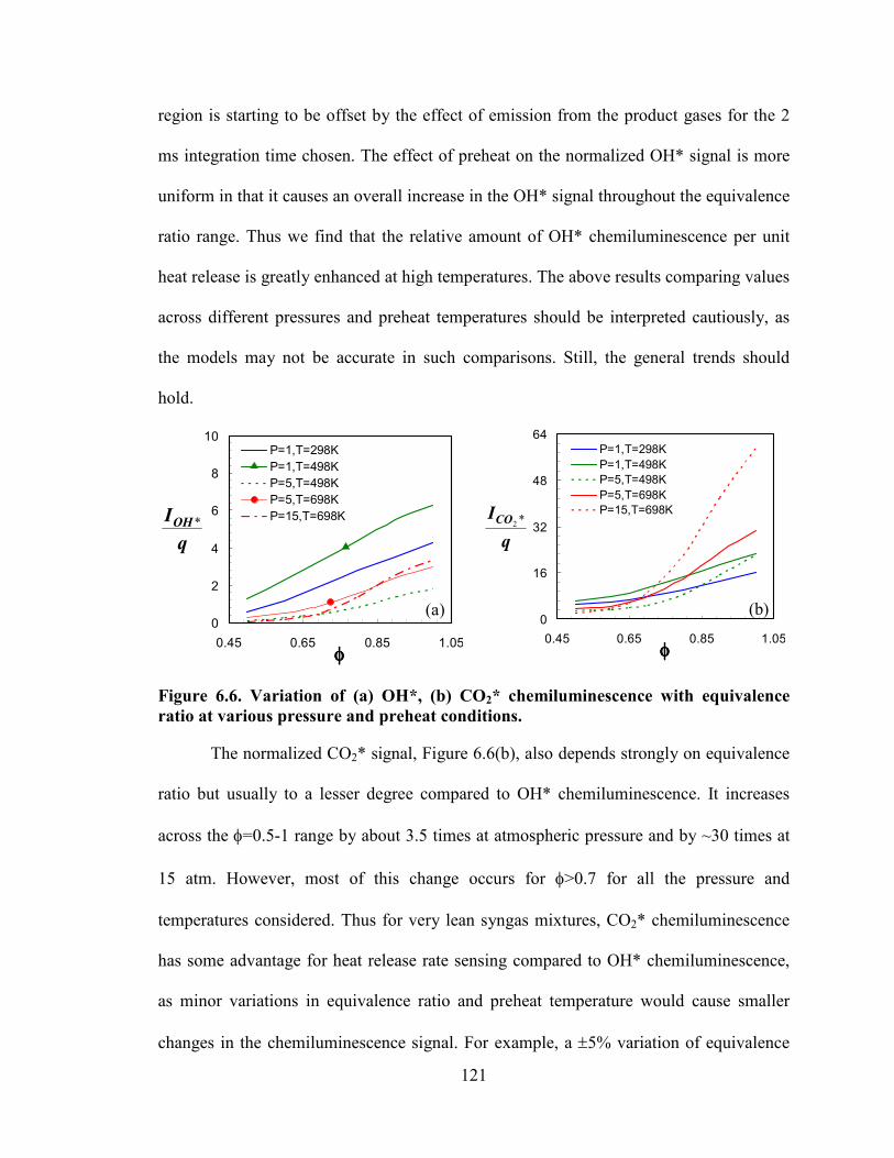
121

region is starting to be offset by the effect of emission from the product gases for the 2

ms integration time chosen. The effect of preheat on the normalized OH* signal is more

uniform in that it causes an overall increase in the OH* signal throughout the equivalence

ratio range. Thus we find that the relative amount of OH* chemiluminescence per unit

heat release is greatly enhanced at high temperatures. The above results comparing values

across different pressures and preheat temperatures should be interpreted cautiously, as

the models may not be accurate in such comparisons. Still, the general trends should

hold.

0

2

4

6

8

10

0.45 0.65 0.85 1.05φφφφ

P=1,T=298K

P=1,T=498K

P=5,T=498K

P=5,T=698K

P=15,T=698K

q

IOH*

0

16

32

48

64

0.45 0.65 0.85 1.05φφφφ

P=1,T=298K

P=1,T=498K

P=5,T=498K

P=5,T=698K

P=15,T=698K

q

ICO *2

(a) (b)

Figure 6.6. Variation of (a) OH*, (b) CO2* chemiluminescence with equivalence

ratio at various pressure and preheat conditions.

The normalized CO2* signal, Figure 6.6(b), also depends strongly on equivalence

ratio but usually to a lesser degree compared to OH* chemiluminescence. It increases

across the φ=0.5-1 range by about 3.5 times at atmospheric pressure and by ~30 times at

15 atm. However, most of this change occurs for φ>0.7 for all the pressure and

temperatures considered. Thus for very lean syngas mixtures, CO2* chemiluminescence

has some advantage for heat release rate sensing compared to OH* chemiluminescence,

as minor variations in equivalence ratio and preheat temperature would cause smaller

changes in the chemiluminescence signal. For example, a ±5% variation of equivalence

122

ratio at φ=0.6 at 15 atm and 700 K, would produce a ±18% change in the CO2* signal per

unit heat release. The same change would produce nearly twice the change (± 30%) in the

OH* signal per unit heat release. The rapid increase in ICO2*/q for higher equivalence

ratios is attributed to the rapid increase in the formation rate of CO2* caused by the rapid

rise in temperature and [O]. It also results from significant amounts of CO2* produced

downstream of the primary reaction zone in the hot products (again when temperature

and [O] are high). This would be even more important in combustors with longer

residence times, as observed earlier (Figure 6.5). In syngas flames as noted previously,

this also occurs for OH*. However, the contribution from the post-flame zone is not as

significant as for CO2*.

The pressure dependence of the normalized CO2* signal is also different. Only at

very lean equivalence ratios does the normalized CO2* signal consistently decrease with

pressure as observed for OH*. Otherwise there appears to be a non-monotonic pressure

effect; an increase in pressure from 1-5 atm reduces ICO2*/q, while a further increase to

15 atm produces a significant rise in the normalized signal. At a given pressure, however,

the CO2* signal per unit heat release responds like the OH* signal to a rise in reactant

temperature; it increases throughout the equivalence ratio range.

6.2.1.1.2 Effect of Aerodynamic Strain Rate

Aerodynamic strain is an important aspect of turbulent flames, and therefore it is

relevant to most practical combustors with high volumetric efficiency. Up to this point in

the thesis, only unstrained laminar flames were simulated. Aerodynamic strain modifies

the residence times of the various species in the flame front, and impacts the diffusion

rates of species and energy. So it is important to gain some understanding on the

123

dependence of chemiluminescence signals on strain rate for interpreting

chemiluminescence data in practical devices.

0

80

160

240

320

400

0 500 1000 1500 2000 2500

Strain Rate, (s-1)

0.0

0.3

0.6

0.9

1.2

1.5

P=1, T=298K

P=1, T=498K

P=5, T=498K

Φ=0.7

q

IOH*

q

ICO *2

Figure 6.7. Strain rate dependence of OH* (solid lines) and CO2* (symbols on lines)

chemiluminescence in H2:CO=50:50 syngas mixture.

A framework for numerical modeling of chemiluminescence in opposed flow,

laminar, premixed strained flames has been previously demonstrated [10]. That approach

is employed here, with the OH* and CO2* signals again normalized by the heat release

rate per unit flame area. However, in this case, the volumetric heat release rate (q’)

profile is integrated up to the stagnation plane.

Simulation results for OH* and CO2* chemiluminescence with varying strain rate,

at different pressure and preheat conditions, are shown in Figure 6.7. The equivalence

ratio of the mixture is fixed at 0.7. The zero strain solution corresponds to that of the one-

dimensional laminar premixed flame. The CO2* signal per unit heat release continuously

decreases with strain for the atmospheric pressure cases. However for the higher pressure

φ=0.7

124

case, the CO2* signal is essentially independent of strain, except for an initial drop from

the zero strain solution. This drop may be due to the difference in the calculation

approaches for the zero strain and strained flames rather than being indicative of a strain

effect. Preheating the reactants does not seem to effect the behavior of the normalized

CO2* signal with strain (other than to increase ICO2*/q as noted previously). Since q

decreases with strain, the results show that the CO2* signal decreases faster than q with

strain. The normalized OH* signal (included in Figure 6.7) also decreases continuously

with strain, except for the room temperature and pressure case. Furthermore, IOH*/q is less

sensitive to strain, decreasing by no more than 11% for the conditions examined, whereas

ICO2*/q changes by 30% for the same strain rate range.*

Summarizing the findings up to this point, OH* chemiluminescence can be

identified as a better heat release marker for turbulent premixed syngas flames at near

stoichiometric conditions. It has a lower strain dependence and is less sensitive to

equivalence ratio variations for these conditions. For leaner conditions, heat release

measurements employing CO2* may be advantageous, due to the lower dependence on

changes in φ and preheat temperature, even though the strain dependence is somewhat

greater.

6.2.1.1.3 Effect of Reactant Product Mixing

The influence of hot products mixing with reactants before combustion occurs is

another aspect of practical combustors that needs to be considered. Exhaust gas

*Thus the results also suggest that the chemiluminescence ratio ICO2*/ IOH* will also decrease with strain.

125

recirculation (EGR) is a popular strategy for NOx control in many practical combustion

devices [79-81]. In addition, reactant-product mixing can also occur as part of the

stabilization processes in combustors. For example in gas turbine combustors, swirl

stabilization and partial lifting of lip- or dump- stabilized flames can produce zones

where product-reactant mixing can occur prior to combustion. Therefore, we examine the

effect of product recirculation on flame chemiluminescence. The fraction of product gas

in the reactants is commonly quantified by an EGR ratio, specifically the mass ratio of

recycled gases to the total mass of the mixture.

Adiabatic product recirculation (denoted hot EGR here) was examined for a

syngas equivalence ratio of 0.7, and for EGR ratios of 5, 11 and 20%. Note, as the EGR

ratio is increased, the inlet temperature of the reactants increases but the final product

temperature remains constant since adiabatic product recirculation is simulated. Results

are shown for the normalized OH* and CO2* chemiluminescence in Figure 6.8. Neither

IOH*/q nor ICO2*/q is appreciably affected by product recirculation. The normalized OH*

signal does increase somewhat with recirculation (by ~10%) for the two atmospheric

pressure cases. For example at 11% EGR, IOH*/q increases by about 6% at 298 K and 9%

at 500 K compared to the 0% EGR case. The effect at higher pressure is even smaller,

IOH*/q is practically constant at 5 atm. The CO2* signal (ICO2*/q) varies only slightly (a

few percent), increasing at 1 atm and decreasing at 5 atm. Reactant preheating does not

change this result. In summary, product recirculation does not appear to significantly

impact the ability of OH* or CO2* chemiluminescence to provide measurements of heat

126

release in syngas fuels.* It is interesting to note that for a given operating condition, the

temperature at which the OH* profile (iOH*) peaks, did not change significantly over the

EGR ratios considered. The same was observed for the CO2* profile.

0

100

200

300

400

0 5 10 15 20 25

EGR %

0

0.3

0.6

0.9

1.2

1.5

1.8

P=1,T=298K

P=1,T=498K

P=5,T=498K

Φ=0.7

q

ICO *2

q

IOH*

Figure 6.8. Dependence of OH* (solid lines) and CO2* (symbols on lines)

chemiluminescence on product recirculation in a H2:CO=50:50 (φφφφ=0.7) syngas mixture.

6.2.1.2 Methane

While chemiluminescence from OH*, CH* and CO2* occur in methane-air, the

CO2* signal is more readily corrupted in practical combustors, for example by other

broadband sources such as HCO chemiluminescence and blackbody radiation sources,

e.g., soot and combustor walls. So, only the normalized OH* (IOH*/q) and CH* (ICH*/q)

chemiluminescence signals are considered in this analysis.

*This also suggests that product recirculation would have little effect on the ratio ICO2*/ IOH*..

φ=0.7

127

6.2.1.2.1 Effect of Pressure and Reactant Preheat

Simulation results for OH* chemiluminescence are presented in Figure 6.9, and it

can be seen that the normalized OH* signal is a strong function of equivalence ratio, as in

the syngas case. IOH*/q increases by six times at atmospheric pressure for 0.6<φ<1. At

high pressure (15 atm), the dependence is even greater, with an increase of ~70 times for

the same equivalence ratio range.

Pressure in general, decreases the normalized OH* signal over the entire φ range.

However, this decrease is more pronounced for leaner mixtures. This effect has been

observed in an earlier experimental study [19]. At a given equivalence ratio and pressure,

preheating also increases the normalized OH* signal, and again the increase is more

pronounced for leaner conditions. Overall, the variation with pressure over typical

operating conditions is more significant than the preheating effect. However,

experimental results in methane-O2/He flames at elevated pressures only indicate a

decrease of OH* signal with pressure consistent with the model predictions but otherwise

reveal a negligible effect of reactant preheat as shown in Figure 5.10.

These results can be explained by examining the OH* formation and destruction

rates. As shown above, R3 dominates the overall formation in low pressure

environments, responsible for almost 80% of the OH* signal at atmospheric pressure. As

R3 formation occurs in the primary reaction zone and because increasing pressure

reduces the flame thickness, the normalized integrated OH* signal associated with R3

decreases with pressure (the actual OH* signal increases, but q increases faster). While it

is true that the contribution from R1 in the product gases increases with pressure

(representing ~50% of the total OH* production at 15 atm), the limited residence time

128

assumed in this simulation limits its effect. Also, lower temperatures for leaner

equivalence ratios reduces mole fractions of the radicals (CH, O and H) necessary for

OH* formation.

0

4

8

12

16

20

0.45 0.65 0.85 1.05φφφφ

0

2

4

6

8P=1, T=298K

P=1, T=498K

P=5, T=498K

P=5, T=698K

P=15, T=698K

q

IOH*

Figure 6.9. OH* chemiluminescence in methane at various pressure and preheat;

the high pressure results are scaled to the right axis.

The dependence of OH* chemiluminescence-based heat release sensing of

equivalence ratio fluctuations can be determined from Figure 6.9. In general, there is less

dependence at near stoichiometric conditions. For example at 15 atm, a ±5% equivalence

ratio fluctuation around a mean value of φ=0.9 would cause a ±20% change in the

sensitivity of chemiluminescence to heat release rate. The same ±5% fluctuation at

φ=0.55, would cause a larger (±30%) change. Similarly for reactant preheat and pressure

fluctuations, the relation between OH* chemiluminescence and heat release shows less

variation at near stoichiometric conditions. For example at 5 atm and a 200 K preheat

change, IOH*/q increases by 35% at φ=1.0 whereas it increases by twice that (70%) at

129

φ=0.7. However, as shown in Figure 5.10, the experiments suggest that at elevated

pressures, the effect of reactant preheat may not be significant and any fluctuations in

preheat would not change the OH* chemiluminescence signal appreciably.

The results for CH* chemiluminescence are shown in Figure 6.10. The

normalized CH* signal increases by as much as 15 times at atmospheric conditions but

only by four times at 15 atm for 0.6<φ<1. Thus in contrast to OH* chemiluminescence

for methane-air flames, the equivalence ratio dependence is reduced for CH* at high

pressure. Experimental results for methane-O2/He flames in Figure 5.13and Figure 5.10

at 10 atm-298 K indicate an increase of ~4 times in CH* signal as compared to ~20

times increase in OH* signal in 0.66<φ<1, consistent with the modeling predictions.

0

3

6

9

12

0.45 0.65 0.85 1.05φφφφ

P=1, T=298K

P=1, T=498K

P=5, T=498K

P=5, T=698K

P=15, T=698K

q

ICH*

Figure 6.10. CH* chemiluminescence in methane at various pressure and preheat

conditions.

Model predictions indicate that reactant preheat produces a uniform increase in

ICH*/q throughout the equivalence ratio range, by 1.5 times at atmospheric pressure.

130

However at 5 atm, a 200 K preheat enhances ICH*/q more for leaner mixtures. Also for a

given temperature and equivalence ratio, pressure decreases ICH*/q, with the decrease

more pronounced near φ=1.0. For example raising the pressure from 5 to 15 atm results in

a drop in ICH*/q of 43% at φ=1.0, but only 20% at φ=0.6. These observations were also

verified experimentally in methane-O2/He flames at elevated pressures. At 5 atm, reactant

preheating clearly increased the CH* chemiluminescence signal in Figure 5.14. Similarly,

comparing the 5 atm and 10 atm results, it can be seen in Figure 5.14 that the CH* signal

decreased by ~4 times, almost uniformly, with increase in pressure. Similar trends were

also observed in an earlier experimental effort [30].

To compare CH* to OH* for heat release sensing under unsteady conditions, e.g.,

combustion instability, we examine the dependence of ICH*/q to fluctuations in

equivalence ratio and reactant temperature. For equivalence ratio oscillations at 15 atm, a

±5% change in equivalence ratio produces a ±15% change in ICH*/q. However similar

fractional changes in equivalence ratio would produce a ±20% fluctuation at φ=0.9 and a

±30% change at φ=0.55 in OH* signal at 15 atm. This suggests that CH* is better suited

for high pressure applications of heat release sensing compared to OH*. However, the

current experimental results in the methane-O2/He flames show that preheating has a

weaker effect on IOH*/q compared to ICH*/q (see Figure 5.10 and Figure 5.13).

6.2.1.2.2 Effect of Aerodynamic Strain

Simulation results for the normalized OH* and CH* signals in an opposed flow

(strained) flame are shown in Figure 6.11 for an equivalence ratio of 0.7. ICH*/q is

somewhat more dependent on strain at atmospheric conditions than IOH*/q. Reactant pre-

131

0

2

4

6

8

10

0 200 400 600 800

Strain Rate, s-1

0.0

0.5

1.0

1.5

2.0

2.5

3.0

P=1, T=298K

P=1, T=498K

P=5, T=498K

q

IOH*

Φ=0.7

q

ICH*

Figure 6.11. Strain rate dependence of OH* (lines) and CH* (lines with symbols)

chemiluminescence in methane-air flames at φφφφ=0.7.

heating makes both signals less dependent on strain. For the high pressure case, both

signals are practically independent of strain. This may be because both preheat and

pressure result in thinner flames, which require higher strain rates to influence the

reaction zone. Similar trends were observed for calculations with a stoichiometric

mixture.

It is interesting to examine the effect of aerodynamic strain rate on the individual

production pathways of OH* and CH*. Simulation results for the relative contributions of

R1 and R3 to the normalized OH* signal and their dependence with strain rate are shown

in Figure 6.12 for an equivalence ratio of 0.7. The OH* production from R1 generally

decreases with strain, whereas strain enhances production for the R3 path.

132

0.0

0.2

0.4

0.6

0.8

1.0

0 200 400 600 800

Strain Rate, s-1

I OH*) R1/q

0

1

2

3

4

I OH*) R3/q

P=1, T=298K

P=1, T=498K

P=5, T=498K

Φ=0.7

Figure 6.12. Strain rate dependence of OH* chemiluminescence produced via R1

(lines) and R3 (lines with symbols) in methane-air flames (φφφφ=0.7).

This is because as strain rate increases, the residence time decreases, and OH*

production via R1 being a strong function of residence time results in a reduction of OH*

signal, as discussed earlier (Table 6.1). Moreover, this residence time effect is more

prominent in near stoichiometric flames. So under stoichiometric conditions, the

normalized OH* signal decreases by as much as 50% compared to the unstrained case,

even at high pressure. Whereas, in case of R3, q decreases faster than IOH* which causes

the increase in the normalized OH* signal. This is because the q’ (heat release rate)

profile is wider than OH* (iOH*) profile in the flame, and therefore strain effects q’ more

than iOH*. Similarly results for the strain dependence of reactions R6 and R7 for CH*

production are given in Figure 6.13. In this case, ICH*/q produced by either R6 or R7

increases with strain irrespective of the pressure and temperature conditions. CH* is only

133

produced in the reaction zone, which causes the increase in the normalized CH* signal

due to reasons similar to those given above.

0.0

0.2

0.4

0.6

0.8

1.0

0 200 400 600 800

Strain Rate, s-1

I CH*) R6/q

0.0

0.5

1.0

1.5

I CH*) R7/qP=1, T=298K

P=1, T=498K

P=5, T=498K

Φ=0.7

Figure 6.13. Strain rate dependence of CH* chemiluminescence produced via R6

(lines) and R7 (lines with symbols) in methane-air flames (φφφφ=0.7).

6.2.1.2.3 Effect of Reactant Product Mixing

Results for OH* and CH* with adiabatic product recirculation are shown in

Figure 6.14 at an equivalence ratio of 0.7. As in the syngas case, the normalized OH*

signal is practically unaffected by product recirculation at the pressure and preheat

conditions studied here. On the other hand, the normalized CH* signal is significantly

affected; it increases by as much as 50% for the 20% EGR case. Higher pressures inhibit

this increase in CH* signal with EGR. In these cases, q increases only by ~5% in the

range of EGR ratios considered. This implies that ICH* increases faster than q. Similar

behavior of OH* and CH* signals is also observed in near stoichiometric flames. EGR,

unlike aerodynamic strain rate, affects the OH* (R1 and R3) and CH* (R6 and R7)

134

production pathways similarly, increasing both. The contributions from R1 and R3 for

OH* increase slightly with EGR, while contributions from R6 and R7 increase as much

as 50% for the atmospheric conditions, in the range of EGRs considered.

0

1

2

3

4

0 10 20 30

EGR %

0

1

2

3

P=1, T=298K

P=1, T=498K

P=5, T=498K

q

IOH*

q

ICH*

Φ=0.7

Figure 6.14. Dependence of OH* (solid lines) and CH* (lines with symbols)

chemiluminescence on product recirculation in methane-air flames (φφφφ=0.7).

Most of the OH* is produced by R3, which has CH as one of its reactants. Both

R6 and R7 responsible for production of CH* have C2H as one of its reactants. However,

OH* is weakly affected by EGR while CH* signal increases noticeably. This only proves

that EGR favors C2H more than CH. It can be seen in Table 6.4 that peak [C2H] increases

as much as 42%, while peak [CH] only increases by 6% , at 1atm 500 K, for a 5%-20%

increase in EGR.

135

Table 6.4. Percentage increase in [CH] and [C2H] peak concentrations for a 5% to

20% increase in EGR for an equivalence ratio of 0.7. Concetration units in mol/cm3.

Operating Conditions [CH] [C2H]

1 atm, 300 K 9.6% 35%

1atm, 500 K 6% 42%

5atm, 500 K 5% 23%

6.2.2 Equivalence Ratio Sensing

As previously noted, experiments reported in the literature for some hydrocarbon

flames at certain conditions showed the variation of chemiluminescence intensity ratios,

such as CH*/OH* or C2/OH*, with equivalence ratio be promising for equivalence ratio

sensing. For this sensing application, it would be preferable that this variation be

monotonic with a good sensitivity (steep slope) for greater reliability and accuracy. The

variation of chemiluminescence intensity ratios in methane and a H2:CO=50:50 syngas

mixture are studied over a range of operating conditions. Experimental results are used to

interpret the modeling results wherever applicable.

6.2.2.1 Syngas

In syngas flames, CO2*/OH* ratio is the only ratio that can be measured. The

computed emission ratios for the syngas mixture considered (H2:CO=50:50) were scaled

with to match the validation data at atmospheric conditions (Chapter 4). For syngas-air

flames at atmospheric conditions, this scaling constant (Cdet) had a value of 20. However,

for syngas flames with O2/He as the oxidizer, at elevated pressure and temperature

conditions, this scaling constant was found to be ~32. This suggests that the models either

under predict CO2* or over predict OH* in such conditions. So, the models can only be

136

used to qualitatively interpret the behavior of the chemiluminescence intensity ratio

CO2*/OH* with equivalence ratio. The CO2* and OH* profiles were spatially integrated

such that they correspond to a combustor residence time of 2-3 ms, which is

characteristic of a number of low NOx combustors.


It can be seen in Figure 4.3 and Figure 4.8 that the variation of CO2*/OH* ratio

with equivalence ratio is similar for syngas flames at various operating conditions. In

general, the CO2*/OH* ratio remains nearly constant for φ>0.7 and then steeply increases

for very lean flames, i.e., φ<0.7. This makes the CO2*/OH* signal ratio of little use for

sensing equivalence ratio, except perhaps at very lean conditions. This is further

illustrated with simulations for a H2:CO=50:50 mixture at different pressure and

temperature conditions (Figure 6.15). The simulated ratios were scaled to the baseline

atmospheric case for convenience. Again, the results in Figure 6.15 should be interpreted

primarily in regard to their φ variation.* Nevertheless, the results clearly indicate that

ICO2*/IOH* would make a poor choice for sensing equivalence ratio in the range of

pressures and temperatures considered.

*For example, the experimental data for a H2:CO~33:67 mixture at φ=0.6 (Figure 4.8), show the ICO2*/IOH*

ratio increasing with pressure, unlike the simulations.

137

0.00

0.05

0.10

0.15

0.20

0.45 0.65 0.85 1.05φφφφ

0.0

0.2

0.4

0.6

0.8

1.0P=1,T=298K

P=1,T=498K

P=5,T=498K

P=5,T=698K

P=15,T=698K

*

*2

OH

CO

I

I

Figure 6.15. Variation of the CO2*/OH* chemiluminescence ratio with equivalence

ratio at various pressure and preheat conditions. The atmospheric results are scaled

with the left axis; the rest of the data scale with the right axis.

6.2.2.2 Methane

In premixed methane flames, ICH*/IOH* has been shown to be a promising

candidate for sensing equivalence ratio at various pressures [30].* As concluded in

Chapter 5, the chemiluminescence models can be used to qualitatively predict the

dependence of the CH*/OH* chemiluminescence intensity ratio with equivalence ratio.

At atmospheric conditions, the computed ICH*/IOH* values were scaled by a constant to

match experimental validation data. This scaling constant is ~24 at room pressure and

* ICO2*/IOH* results presented in Chapter 5 at atmospheric conditions show this ratio to be non-monotonic

and only weakly sensitive to φ; thus it is not considered here.

138

temperature conditions in methane-air flames. However, at elevated pressure conditions

(and with the He/O2 oxidizer), this scaling constant was between 0.5 and 2.


In Chapter 5, the chemiluminescence intensity ratio ICH*/IOH* was seen to

monotonically increase with equivalence ratio for atmospheric pressure conditions.

However, the variation of ICH*/IOH* was not the same at elevated pressures. For example,

it can be seen in Figure 5.14 that at 10 atm the ratio is decreasing, while at 5 atm it is

closer to constant throughout the equivalence ratio range. Figure 6.16 provides further

indication of this with simulation results at a range of pressure and temperature

conditions for methane-air flames. The simulated chemiluminescence ratios are scaled

with the Cdet value determined from the baseline atmospheric results. At atmospheric

pressure, ICH*/IOH* monotonically increases as expected. At 5 atm, there is little change in

ICH*/IOH* with equivalence ratio (similar to what was observed in methane-He/O2 flames),

except for very lean conditions, i.e., φ<0.65. This suggests that ICH*/IOH* cannot be used

for sensing equivalence ratio in some conditions. At even higher pressures (15 atm),

ICH*/IOH* again varies significantly with φ, now decreasing monotonically (again in

agreement with the methane-He/O2 validation experiments). According to Figure 6.16,

pressure generally increases the magnitude of the ICH*/IOH* ratio, at a given equivalence

ratio, whereas the validation experiments indicated the opposite effect. Similarly, the

models predict that preheating generally has a decreasing effect on the ICH*/IOH* ratio,

though the decrease is less than 20% for most of the cases considered. However, in the

high pressure experiments, preheating produced an increase in ICH*/IOH*. In summary,

ICH*/IOH* can be used for sensing equivalence ratio only at certain conditions, and the

139

changing relationship between ICH*/IOH* and φ with pressure must be taken into account.

Such trends have been observed experimentally without reactant preheating [30].

0.0

0.1

0.2

0.3

0.4

0.5

0.45 0.65 0.85 1.05φφφφ

0

2

4

6

8

10

12

14P=1, T=298K

P=1, T=498K

P=5, T=498K

P=5, T=698K

P=15, T=698K

*OH

*CH

I

I

Figure 6.16. CH*/OH* chemiluminescence ratio in methane-air flames at various

pressures and preheat; the high pressure results are scaled to the right axis.

6.2.2.2.2 Effect of Aerodynamic Strain

Results for ICH*/IOH* variations with strain rate are given in Figure 6.17 at φ=0.7

and 1. It was noted in Chapter 5 that CH* chemiluminescence is more dependent on

strain than OH*. This is clearly evident here, where ICH*/IOH* increases with strain rate.

For a given strain rate, the increase in ICH*/IOH* is almost the same for both equivalence

ratios considered, except at high pressure. The maximum increase of 13% occurs at

ambient pressure conditions, while for the higher pressure and preheat case, ICH*/IOH*

ratio increases by 1% for the lean case and increases by about 10% for the stoichiometric

case. However, with ICH*/IOH* varying by only 10% over a wide range of strain rates, it

can be concluded that ICH*/IOH* is not very sensitive to strain rate. This is supported by

140

the agreement between results in laminar and turbulent flames at atmospheric conditions

presented in Chapter 5 for conditions away from the lean blow out limit of the swirl

combustor.

0.0

0.2

0.4

0.6

0.8

1.0

1.2

0 500 1000 1500 2000

Strain Rate, s-1

P=1, T=298K

P=1, T=498K

P=5, T=498K

*OH

*CH

I

I

Figure 6.17. Dependence of CH*/OH* ratio with strain rate for φφφφ=1 (dashed line) and φφφφ =0.7 (solid line).

6.2.2.2.3 Effect of Exhaust Gas Recirculation

Results for ICH*/IOH* variation with product recirculation are shown for the same

two equivalence ratios, 0.7 and 1. It was demonstrated above that the CH* signal

increases with product recirculation while OH* signal is practically unaffected by it. It

can be see that ICH*/IOH* increases with product recirculation. For φ=0.7 and 20% EGR,

ICH*/IOH* increases by 27% at 5 atm and 498 K, while at 1 atm and for both 298 and

498 K reactant temperatures, the ratio increases more. Similar results are observed for the

stoichiometric case. However, for lower levels of product mixing (EGR<5%), the effect

on ICH*/IOH* is negligible.

141

6.3 Other Considerations

6.3.1 Thermal Excitation

As mentioned earlier, in addition to chemical formation of the excited states,

thermal excitation can also occur. The contribution of thermal OH* and CH* emission

for sensing is therefore analyzed here. The procedure for calculating the upper estimate of

thermal OH* based on equilibrium calculations is already outlined (Chapters 4 and 5).

That methodology along with the assumption that the formation reactions are accurate in

predicting the absolute concentrations of OH* and CH* is used to estimate the thermal

contributions in methane-air flames.


methane-air flames for different residence times and equivalence ratios.

% Thermal OH for 2-3 ms % Thermal OH for 10 ms Pressure and

Temperature φ = 0.7 φ = 1.0 φ = 0.7 φ = 1.0

1 atm, 298 K 0.01 0.43 0.035 2.63

1 atm, 498 K 0.08 1.62 0.30 8

5 atm, 498 K 0.51 12 2 29

5 atm, 698 K 3.1 23.7 10.9 39

15 atm, 698 K 11.5 38 28.7 46

Results for thermal OH* as a fraction of the total OH* emission for premixed

methane flames are presented in Table 6.5. The thermal OH* is seen to be a function of

residence time and the equivalence ratio of the combustor (as thermal OH* is formed

primarily in the hottest regions). However, the thermal contribution to the total OH*

142

signal also rises significantly with pressure.* Hence in high pressure combustors,

especially combustors with long residence times and near stoichiometric conditions, the

OH* emission has to be treated carefully.

Results for thermal CH* as a fraction of the total CH* for premixed methane-air

flames are presented in Table 6.6. As CH and CH* exist primarily in the thin reaction

zone for lean flames, a residence time of 2-3 ms was considered, which is more than

sufficient to capture the complete reaction zone in all cases. It can be clearly seen that

thermal CH* is practically negligible at these conditions, as expected. Thermal CH* may

become important in oxy-methane flames [32].

Table 6.6. Thermal CH* contribution (as percentage of the total CH* signal) in

methane-air flames.

% Thermal CH for 2-3 ms Pressure and

Temperature φ = 0.7 φ = 1.0

1 atm, 298 K 0.006 0.06

1 atm, 498 K 0.012 0.08

5 atm, 498 K 0.007 0.13

5 atm, 698 K 0.02 0.19

15 atm, 698 K 0.012 0.24

6.3.2 OH* Self-Absorption

Example calculations are shown in Table 6.7 for the effect of self-absorption on

OH* emission in methane-air combustion at various temperature and pressure conditions

for a residence time of 2.5 ms. A conservative estimate of these values is computed using

* As described in a previous section, the chemical formation of OH*, normalized by heat release, decreases

at high pressures.

143

Eq. (3) (Chapter 2) and peak absorbance coefficient is used for the R-branch bandhead of

the OH (A-X) (0,0) transition without considering the line shapes/profiles. However, this

calculation is useful to access the conditions in which self-absorption may be important.

It can be seen that the impact of self-absorption can be important at elevated pressures

and temperature conditions, particularly near stoichiometric equivalence ratios. It should

be expected that self-absorption would increase with the simulated residence time of the

combustor (which is used here to determine the emission path length). So, it would be

wise to place the sensor/detector on the reactants side of the flame.

Table 6.7. Fraction of OH* signal absorbed in methane-air flames at different

pressure and temperature conditions.

% Absorption

(t=2.5ms)

Methane/Air

Flames

φφφφ = 1.0 φφφφ = 0.7

1atm-300K 7 1 1atm-500K 11 3.7

5atm,-500K 18 3.2

5atm-700K 34 11

15atm-700K 39 13

6.3.3 CO2* Background

In most sensing and combustion diagnostic applications, flame

chemiluminescence is acquired with spectral filters placed in front of detectors such as

photomultiplier tubes, photodiodes or CCD cameras. At best (e.g., for interference

filters), their bandpass is ±5-10 nm about the center wavelength. It is also well known

that CO2* background is present in the 200-600 nm region [55]. Thus, it underlies the

other (OH* and CH*) emission signals. So unless a spectrometer or additional detector is

used to monitor the CO2* background, its contribution can not be removed from the

144

detected signal. Thus it is interesting to estimate the contribution of the CO2* background

to the total signal at OH* and CH* wavelengths. For this purpose, the resolved flame

spectra from the swirl-stabilized methane combustor at atmospheric pressure and laminar

CH4-O2/He flames at elevated pressure are analyzed to study the CO2* background. The

OH* signal, SOH*, was found by integrating the (0,0) band over a 5 nm bandwidth

centered at the OH* peak (~309 nm). The CH* signal, SCH*, was found by integrating the

430 nm CH band over a bandwidth of 5 nm. The CO2* background over the same 5 nm

bandwidths was approximated by the means of a cubic polynomial. The area under this

polynomial was taken as the estimate for the CO2* background. Results for atmospheric

swirl flame and laminar flames at elevated pressure are shown in Figure 6.18.

0

20

40

60

80

100

0.6 0.7 0.8 0.9 1 1.1

φφφφ

% CO2* Contribution

OH*

CH*

0

20

40

60

80

100

0.5 0.7 0.9 1.1φφφφ

% CO2* Contribution

5atm-T300

5atm-T600

10atm-T300

Figure 6.18. CO2* contribution in methane flames to OH*(309±5nm) and CH*

(431±5nm) signals; (a) atmospheric pressure and (b) elevated pressure.

It is evident that the CO2* background affects the CH* signal more than the OH*

signal. For example at φ=0.8 at atmospheric conditions, only 30% of the total signal at

the CH* wavelength is from CH* chemiluminescence, while OH* chemiluminescence

makes up 80% of its total signal. Moreover, the CO2* background has a weaker

equivalence ratio dependence for OH* chemiluminescence than for CH*. At elevated

OH*

CH*

(a) (b)

145

pressures, this dependence is reduced for CH* too, but interestingly the CO2* background

increases with φ at 10atm. Another interesting aspect is to consider the variation of

chemiluminescence intensity ratio with equivalence ratio, which has a direct bearing on φ

sensing. It can be seen in Figure 6.19 that the background corrected SCH*/SOH* has a

higher sensitivity, i.e., it varies by a factor of ten in the φ range considered. Whereas,

SCH*/SOH* without background correction only varies by a factor of two. So, a sensor

based on the background corrected ratios would be more sensitive to changes in φ. The

high pressure experimental data also support this fact. Moreover, SCH*/SOH* is almost

constant near the lean blow out regime of the swirl combustor if background correction is

not considered and as such cannot be used to sense the proximity of the combustor to lean

blow off..

It is possible, though, that the uncorrected normalized signals could have a

different φ dependence which might make them more advantageous to use for heat

release sensing than the background corrected normalized chemiluminescence signals. To

verify this possibility, both background corrected and uncorrected signals are considered

for OH* and CH* in Figure 6.20. The uncorrected signals are multiplied by a single

multiplier so as to minimize the least square difference between the two signals. As seen

in Figure 6.20a, there is practically no difference in the φ dependence for the OH* signal

without background correction. However for CH* chemiluminescence, failing to correct

for the background at 10 atm increases the systematic error for heat release sensing

associated with φ changes (Figure 6.20b).

146

0.0

0.2

0.4

0.6

0.8

0.6 0.7 0.8 0.9 1 1.1

φφφφ

*

*

OH

CH

S

S

Figure 6.19. Comparison of chemiluminescence intensity ratio for CH* and OH*:

with background correction (closed symbols); without background correction (open

symbols).

0

3

6

9

12

15

0.5 0.7 0.9 1.1φφφφ

5atm-T300

5atm-T600

10atm-T300

f

OH

m

S

&

&*

0

1

2

3

4

0.5 0.7 0.9 1.1φφφφ

5atm-T300

5atm-T600

10atm-T300

f

CH

m

S

&

&*

(a) (b)

Figure 6.20. Variation of normalized (a) OH* and (b) CH* chemiluminescence

signals at elevated pressure conditions. Background corrected signals (closed

symbols) and uncorrected signals (open symbols).

147

CHAPTER 7

CONCLUSIONS AND RECOMMENDATIONS

7.1 Summary and Conclusions

The primary objective of this thesis was to identify and validate existing

chemiluminescence mechanisms for OH*, CH* and CO2* for combustion conditions.

This involved a comparison of experimental data with simulation results based on the

different mechanisms. Systematically acquiring global (spatially integrated) OH*, CH*

and CO2* chemiluminescence data from simple laminar premixed flames formed the

main focus of the experimental investigation. Experiments were carried out for a range of

operating conditions, including variations in pressure, reactant preheat temperature,

equivalence ratio (φ), dilution, and fuel composition: H2-CO syngas mixtures, methane

and Jet-A; to test the robustness of the chemiluminescence mechanisms. Detailed

numerical simulations for unstrained, 1-d laminar flames were performed with leading

chemical kinetic mechanisms relevant to the above fuels. The spatially resolved

simulation results were integrated to provide a comparison to the experimental data.

Laminar flames were used in part to provide a meaningful comparison between the

experiments and simulations. Global chemiluminescence intensity ratios and global

chemiluminescence signals normalized with fuel mass flow rate were used for validating

the chemiluminescence mechanisms.

148

For CO2* chemiluminescence, a global reaction rate was derived, based on the

spectral data of Slack et al. [55], for the photon emission rate at 375 nm, which is given

by the following.

( )nmscm

molOCO

T

KiCO ⋅⋅

−×±=′

3

3 ]][][2300

exp[103.03.3*2

This model produced excellent agreement with the experimental data for syngas (both

atmospheric and high pressure) and methane (atmospheric) flames. While this

mechanism produced the correct variation with equivalence ratio at high pressure, it did

not produce the correct scaling for a given φ with pressure. This is attributed to

inaccuracies in the basic chemical reaction mechanism used in the high pressure

simulations, as well as signal loss due to radiative trapping (by species such as CO2 and

H2O). For the Jet-A flames and high pressure methane flames, the CO2* background at

375 nm had significant interferences from other emitters, possibly HCO and water.

Two OH* formation reactions were found to be needed to accurately predict the

validation results. R1 (O+H+M) is the dominant formation reaction in H2 systems and in

the post-flame product gases of hydrocarbon flames, while R3 (CH+O2) dominates in the

reaction zone for hydrocarbon fuels. The rate constants for both reactions are summarized

in Table 7.1. The temperature dependence for k1 was chosen to be the expression given in

[37] as it provided the best results in the syngas tests. The pre-exponential factor given is

based on the range of k1 values reported in the literature. The k3 temperature dependence

determined from the atmospheric methane-air and Jet-A flame validations is the

expression given in [45]. From comparison of the atmospheric syngas and methane

results, the ratio k1/k3 was estimated, and used to determine the pre-exponential factor for

k3 shown in Table 7.1. This mechanism was able to accurately predict OH*

149

chemiluminescence variations with equivalence ratio and pressure, but failed to correctly

model the influence of reactant preheating (at least in the high pressure methane flames

studied). Possible sources for this discrepancy include radiative trapping of the OH*

emission and the formation of OH* via thermal excitation in the high pressure conditions.

For CH*, two formation reactions, R6 (C2H+O) and R7 (C2H+O2), were

sufficient to predict the experimental data in the lean flames studied here. Two sets of

rate constants (attributed to Peeters [64] and Carl [66]) performed well in the methane

and Jet-A validations, and both are reported in Table 7.1. Both predicted the equivalence

Table 7.1. Validate formation reactions and rate constants for OH* and CH*

chemiluminescence. Rate coefficients are expressed as k = A Tb exp(−−−−Ea/RT) with Ea

in units of cal mol-1 and AT

b in cm

3mol


6mol

-2s-1 for

three body reactions (with T in K units).

# Reaction A b Ea

OH*

R1 H + O + M ↔ OH* + M 4.3(±1.7) × 1014 0.0 6940

R3 CH + O2 ↔ OH* + CO 8.3(±3.4) × 1013 -0.4 4150

CH* (Peeters)

OH* R6 C2H + O ↔ CH* + CO 1.08(±0.4) × 1013

0 0

R7 C2H + O2 ↔ CH* + CO2 2.17(±0.8) × 1010 0 0

CH* (Carl)

OH* R6 C2H + O ↔ CH* + CO 6.02(±3.0) × 1012

0 457

R7 C2H + O2 ↔ CH* + CO2 6.02 × 10-4 4.4 -2285

ratio and preheat dependence, though the Peeters rate constants performed better for very

lean atmospheric conditions, while the Carl rates provides a better match at high pressure.

However, both failed to capture the pressure dependence, which might be due to the lack

of accurate quenching data or inaccuracies in the basic reaction mechanism for estimating

the precursor species (e.g., C2H). Because CH* is formed from C2H, it is only produced

150

in the reaction zone (at least for lean flames). Moreover, thermal excitation of CH* was

negligible for the experimental conditions.

With the validated chemiluminescence mechanisms, there is now a way to

analyze the fundamental behavior of chemiluminescence in combustion systems.

Therefore, the second objective of this thesis was to use the simulation (and

experimental) results to evaluate chemiluminescence for sensing heat release and

equivalence ratio at various operating conditions. The influences of pressure, reactant

preheat, strain and (adiabatic) exhaust gas recirculation were studied for a syngas fuel

(H2:CO=50:50) and for methane. Even though laminar flame data and simulations were

used to analyze chemiluminescence sensing, the excellent agreement between the laminar

methane and turbulent swirl flame experiments suggests that the findings reported here

have relevance to many practical combustor systems. For highly turbulent combustors

where questions regarding the validity of flamelet approaches arise, the validated

mechanisms can be incorporated into detailed turbulence simulations (incorporating

appropriate detailed chemistry) in order to study chemiluminescence in those systems.

In the syngas mixture, both the normalized OH* and CO2* signals vary

significantly with equivalence ratio, which implies that neither are ideal for heat release

sensing. The simulations indicate that both product recirculation and aerodynamic strain

rate do not have any significant effect on either OH* or CO2* chemiluminescence signals

at high pressure and temperature conditions. With respect to heat release rate sensing in

syngas fuels, CO2* appears to be a better option at very lean equivalence ratio conditions

(φ < 0.7), as it has the least sensitivity to equivalence ratio, pressure and temperature

changes. At near stoichiometric conditions, OH* would be a better heat release marker as

151

it is less sensitive to φ variations at these conditions. The chemiluminescence intensity

ratio CO2*/OH* would be of little use for sensing equivalence ratio in syngas

combustion, except perhaps at very lean conditions.

In methane-air flames, the normalized OH* signal is a strong function of

equivalence ratio, as in the syngas case, and hence not ideal for heat release sensing.

Pressure in general, decreases the normalized OH* signal over the entire φ range, with

the decrease more pronounced for leaner mixtures. The simulations indicate that reactant

preheating increases the normalized OH* signal throughout the equivalence ratio range,

though this was not observed in the experiments. For CH*, the φ dependence is reduced

at high pressure, unlike OH*, which is consistent with the experimental observations.

Reactant preheating also increases the CH* chemiluminescence normalized by the heat

release. Also, the normalized CH* signal decreases with an increase in pressure. Both

normalized OH* and CH* signals increase with strain rate at atmospheric conditions, but

are practically independent of strain rate at high pressure and preheat conditions. Product

recirculation has practically no effect on the normalized OH* signal but the normalized

CH* signal increases by as much as 50% for a 20% EGR at an equivalence ratio of 0.7.

These results suggest that CH* is better suited for high pressure applications of heat

release sensing compared to OH*, but the current experimental results in methane-O2/He

flames show that preheating has a weaker effect on IOH*/q compared to ICH*/q.

The CH*/OH* ratio can be used for equivalence ratio sensing only at certain

conditions in methane combustion as this ratio can change from monotonically increasing

(at atmospheric conditions) to monotonically decreasing (at very high pressure), with an

intermediate pressure region that shows little sensitivity to φ. Strain rate has a negligible

152

effect on the chemiluminescence intensity ratio, while %EGR was shown to increase the

magnitude of the CH*/OH* ratio.

The contribution of thermally produced OH* to the overall OH* signal was also

calculated based on equilibrium conditions for methane systems. It was found that the

thermal pathway is not very significant at atmospheric and intermediate pressures, but it

becomes increasingly important at high pressures with large residence times and near

stoichiometric conditions. On the other hand, thermal CH* is practically negligible even

at high pressure and high temperature conditions. The conditions favorable for thermal

OH* production are also favorable for OH* self absorption. So, a sensor placed on the

reactant side of the combustor will be less prone to errors due to radiative trapping. Still,

the OH* signal should be carefully interpreted in high pressure systems with long optical

path lengths.

The contribution of CO2* background to the total signal at the OH* and CH*

wavelengths was studied for methane. For the conditions considered, the CO2*

background made up only a small fraction (~20%) of the total OH* signal, but

contributed as much as 70-90% of the nominal CH* signal. The uncorrected normalized

OH* and CH* chemiluminescence signals do not offer any advantage for heat release

sensing applications. Similarly, the background corrected SCH*/SOH* ratio has a higher

sensitivity to φ compared to measurements without background correction. Thus, it is

advisable to use background corrected OH* and CH* signals for sensing purposes.

For very high pressure combustion, such as in gas turbines (20-50 atm) and

rockets (70 atm and higher), the signal per unit heat release drastically decreases with

pressure. This might be an issue, especially for CH*, if background corrected signals are

153

not used. For OH*, self-absorption and thermal excitation may become increasingly

significant. Moreover, OH* would be produced predominantly in the product gases rather

than the reaction zone (where most of the heat release happens) and hence, may not be

useful for sensing heat release at these conditions.

7.2 Recommendations for Future Work

For chemiluminescence modeling to be applicable for a wide range of operating

conditions, it is necessary for the mechanisms to be robust and well-validated. There is

still some ambiguity in choosing the CH* chemiluminescence mechanism as both the

very different Peeters and Carl rate constants produce excellent agreement with the

experimental data for most of the conditions. As it is necessary to identify the correct rate

constants, more experiments should be carried out, preferably in flames that have a

different [O]/[O2] distribution compared to atmospheric methane-air flames. To select

one of the two mechanisms will require experiments at elevated pressures, or possibly

with a different oxidizer. For example, simulation results for normalized CH* in methane

flames with an equimolar mixture of O2-N2 as oxidizer are shown in Figure 7.1. The

simulations with Carl and Peeters mechanisms were scaled by the same constants that

were used for matching the atmospheric experimental data in methane-air flames. It can

be seen that these conditions clearly differentiate the mechanisms especially for the near-

stoichiometric equivalence ratios.

154

0

20

40

60

80

0.5 0.7 0.9 1.1

φφφφ

Carl

Peeters

f

CH

m

S

&

&*

Figure 7.1. Normalized CH* chemiluminescence in oxy-methane flames at

atmospheric pressure and temperature. Suggested approach for differentiating CH*

chemiluminescence mechanisms. Oxidizer is an equi-molar mixture of O2 and N2.

Most of the data presented in this work at elevated pressure and temperatures was

preliminary and more extensive investigation has to be undertaken to understand various

issues affecting the flame chemiluminescence at these conditions and the inability of

chemiluminescence mechanisms to predict the experimental results quantitatively. The

reason may lie in the failure to accurately model the relative affects of the following

processes: thermal excitation, radiative trapping and collisional quenching of the excited

species. However, accurately estimating the concentration profiles of the relevant

precursor species is also very important. Therefore, more data at different pressure and

temperature conditions would aid in further understanding of these issues.

To apply chemiluminescence modeling to realistic combustors, it is necessary to

understand the dependence of chemiluminescence on the degree of turbulence. So, more

experiments have to be performed in turbulent flames.

155

Very limited chemiluminescence data is presented for laminar premixed

prevaporized Jet-A flames, in this thesis. Jet-A fuel being very relevant in aero-

propulsion devices demands further investigation. More experiments should be

performed at different conditions to validate the OH* and CH* chemiluminescence

mechanisms as well as the basic chemistry for Jet-A combustion. Whether, the

mechanisms provide good agreement or not, these experiments will provide valuable

chemiluminescence data for Jet-A flames at various operating conditions that can be

investigated for φ and heat release sensing applications.

C2* is another prominent emitter in rich methane flames and for higher order

hydrocarbon fuels in the UV-VIS region of the electromagnetic spectrum. The

chemiluminescence intensity ratio C2*/OH* and C2*/CH* has been shown previously to

be useful for equivalence ratio sensing in hydrocarbon flames (see Appendix A).

However, most of the experimental investigation was carried out in methane flames at

atmospheric conditions. There exists a need to study C2* chemiluminescence for φ and

heat release sensing at different operating conditions and in liquid fuels of interest such as

Jet-A. Additionally, little progress has been made in modeling C2* chemiluminescence in

flames and currently only one low pressure flame study has suggested a complete C2*

mechanism [82]. However, the mechanism has huge uncertainties and needs to be

validated further.

156

APPENDIX A

C2* BACKGROUND

The blue green Swan band emission system is typically found in hydrocarbon

flames and is also of great interest in astrophysics as it is part of the emission spectra

from comets and deep space [1]. C2 kinetics are responsible for the production of C2H,

which in turn is an important precursor for the formation of excited CH (A2∆) species.

The following reactions are identified as the possible formation reactions:

CH + CH → C2* + H2 (R8)

C + CH → C2* + H (R9)

C + CH2 → C2* + H2 (R10)

C3 + O → C2* + CO (R11)

C + C2O → C2* + CO (R12)

R8 has been ruled out in flames [83]. A shock heated methane study favors R9 and R10

[84]. A flow discharge study in C2H2/O/H system confirms R10 as the main production

step [61]. R11 and R12 are also reported to occur [85, 86]. The quenching rate

information of the excited C2 species is not well known and is limited to some noble

gases and simple species such as Ar, H, H2, O2 etc [87]. Recently, collisional cross-

sections for collisional quenching of C2(d3Π) by n-alkanes (n=1-8) were measured at

room temperature and low pressure (15 torr) conditions [88].

157

Though the Swan band system was extensively investigated, very little progress

has been made in the development of a C2 chemiluminescence mechanism, modeling the

formation and destruction kinetics of the excited C2 radical. In a recent laser-induced

fluorescence study, collisional quenching rates of the excited state C2(d3Π) were derived

based on the measured fluorescence decay rates, which were then used to deduce the rate

constants for the excited state C2(d3Π) formation reactions from low pressure flame

studies [82]. Rate constants for R10 and R11 were determined along with an estimation

of the overall quenching rate. However, there is significant uncertainty in the rates of

these reactions. This study also estimated the reaction rate parameters for important

reactions of C3, C3H, C3H2 and C2O along with the addition of C and C2 chemistry to

GRI Mech 3.0 mechanism. However, further improvements for the C2* kinetics are

needed to model C2* chemiluminescence accurately.

The chemiluminescence intensity ratio C2*/CH* and C2*/OH* can be used to

sense equivalence ratio in liquid and gaseous systems with the ratio C2*/OH* observed to

be more sensitive to changes in φ [89]. However, a recent study in counterflow premixed

natural-gas flames indicates that C2*/CH* is strongly affected by strain rate and may not

be suitable for sensing equivalence ratio [24]. Likewise, if the normalized C2*

chemiluminescence signal variation with φ was considered, it was shown that C2* would

be more advantageous than OH* or CH* for sensing heat release rate for lean conditions

at room pressure and temperature conditions [24]. Most of the C2* chemiluminescence

results are confined to atmospheric methane flames. Experimental data for C2*

chemiluminescence is severely lacking at elevated pressure and preheat conditions.

158

APPENDIX B

SPECTRAL RESPONSIVITY

Spectral responsivity of the spectrometer, ICCD camera system was estimated

based on intensity measurements from a calibrated OrielTM

QTH 1000W FEL tungsten

halogen light source. The calibration of the light source is accurate to within ±15%.

Acton Spectra-Pro 300i spectrometer with 300 grooves/mm grating (500 nm blaze angle)

coupled with a 16-bit, 1024×256 intensified CCD camera (PI-MAX, 25 mm intensifier)

constitutes the detection system. A fiber optic array consisting of four bundles, each

bundle having three 200µm fused silica fibers with a numerical aperture of 0.22 was

connected to the entrance slit of the spectrometer. The optical fibers have negligible

transmission losses (~1-3%) in the UV-VIS wavelength region of interest (300-500 nm).

The slit width of the spectrometer was set to 100 µm. The intensifier gain was set to 80

and the exposure time was 10 µs. Flatfield function for each fiber bundle was also

measured as part of this study using a 632.8 nm He-Ne laser and moving the spectrometer

grating such that the He-Ne laser peak traversed across the horizontal pixel range (32-

952). The pixels 1-31 and 953-1024 were ignored as they are very close to the edge of the

CCD chip. It should be noted that the flatfield function is only dependent on the spatial

location of the detector pixel and not on wavelength. Moreover, for each fiber, a

rectangular region of 1024×50 pixels was binned vertically to form one composite strip

(1024×1). The flatfield function and the spectral responsivity of the system were

159

estimated for this composite strip. So, for a given incident beam with energy Eo,λ, the

spectrometer-ICCD camera would output a beam with energy is given by

)()(,

λ=λ

λ SRxFFE

E

o

. (23)

where, FF(x) is the absolute flatfield function which only depends on the spatial location

of the beam image on the detector and SR(λ) is the absolute spectral responsivity of the

system. However, the flatfield function was estimated relative to the center pixel i.e. pixel

512 for each fiber and similarly spectral responsivity of the system was estimated relative

to that at 407nm. Theoretical spectral responsivity (TSR) was also calculated based on

the nominal quantum efficiency of the ICCD camera and the typical efficiency of the

spectrometer grating (both obtained from the manufacturer). TSR is the product of these

efficiencies either based on photon (intensity) or power (energy) units. It can be seen in

Figure B.1 that the normalized experimental and theoretical spectral responsivity values

(based on power) have a reasonable agreement. It can be observed that the spectral

responsivity can change by a factor of 2 at most from ~300 nm (OH*

chemiluminescence) to ~430 nm (CH* chemiluminescence).

160

0

0.2

0.4

0.6

0.8

1

1.2

250 350 450 550 650

λ λ λ λ (nm)

Spectral Responsivity

Figure B.1. Relative spectral responsivity of the spectrometer-ICCD camera

detector system. Theoretical (lines); Experiments (symbols).

161

REFERENCES

1 Gaydon, A. G. and Wolfhard, H. G., “Flames: Their Structure, Radiation, and

Temperature,” Fourth edition, Chapman and Hall, 1978.

2 Stojkovic, B. D., Fansler, T. D., Drake, M. C. and Sick, V., “High-speed imaging of

OH* and soot temperature and concentration in a stratified-charge direct-injection

gasoline engine,” Proceedings of the Combustion Institute, vol. 30, pp. 2657-2665,

2005.

3 Schefer, R. W., “Flame sheet imaging using CH chemiluminescence,” Combustion

Science and Technology, vol. 126 (1-6), pp. 255-270, 1997.

4 Muruganandam, T. M., Kim, B.-H., Morrell, M. R., Nori, V., Patel, M., Romig B.

W. and Seitzman, J. M., “Optical equivalence ratio sensors for gas turbine

combustors,” Proceedings of the Combustion Institute, vol. 30, pp. 1601-1609,

2005.

5 Lee, J. G., Kim, K. and Santavicca, D. A., “Measurement of equivalence ratio

fluctuation and its effect in heat release during unstable combustion,” Proceedings

of the Combustion Institute, vol. 28, pp. 415-421, 2000.

6 Luque, J., Jeffries, J. B., Smith, G. P., Crosley, D. R., Walsh, K. T., Long, M. B. and

Smooke, M. D., “CH(A-X) and OH(A-X) optical emission in an axisymmetric

laminar diffusion flame,” Combustion and Flame, vol. 122, pp.172-175, 2000.

7 Smith, G. P., Luque, J., Park, C., Jeffries, J. B. and Crosley, D. R., “Low pressure

flame determinations of rate constants for OH(A) and CH(A) chemiluminescence,”

Combustion and Flame, vol. 131 (1-2), pp. 59-69, 2002.

8 Kojima, J., Ikeda, Y. and Nakajima, T., “Basic aspects of OH(A), CH(A), and C2(d)

chemiluminescence in the reaction zone of laminar methane-air premixed flames,”

Combustion and Flame, vol. 140, pp. 34-45, 2005.

9 Haber, L. C., Vandsburger, U.,. Saunders, W, R. and Khanna, V. K., “An

examination of the relationship between chemiluminescent light emissions and heat

162

release rate under non-adiabatic conditions,” Proceedings of International Gas

Turbine Institute, 2000.

10 Samaniego, J. M., Egolfopoulos, F. N. and Bowman, C. T., “CO2*

chemiluminescence in premixed flames,” Combustion Science and Technology, vol.

109, pp. 183-203, 1995.

11 Gaydon, A. G. and Wolfhard, H. G., “Comparison of the spectra of turbulent and

laminar flames,” Fuel, vol. 33 (3), pp. 286-290, 1954.

12 John, R. R., Wilson, E. S. and Summerfield, M., “Studies of the mechanism of flame

stabilization by a spectral intensity method,” Jet Propulsion, vol. 25 (10), pp. 535-

537, 1955.

13 Clark, T. P., “Studies of OH, CO, CH and C2 radiation from laminar and turbulent

propane-air and ethylene-air flames,” NACA TN 4266, 1958.

14 Kojima, J., Ikeda, Y. and Nakajima, T., “Spatially resolved measurement of OH*,

CH* and C2* chemiluminescence in the reaction zone of laminar methane/air

premixed flames”, Proceedings of the Combustion Institute, vol. 28, pp. 1757-1764,

2000.

15 Docquier, N., Lacas, F. and Candel, S., “Closed-loop equivalence ratio control of

premixed combustion using spectrally resolved chemiluminescence measurements”,

Proceedings of the Combustion Institute, vol. 29, pp 139-145, 2002.

16 Yamazaki, M., Ohya, M. and Tsuchiya, K. Int. Chem. Eng. vol. 30, pp. 160-168,

1992.

17 Brown, M. S., Meyer, T. R., Sturgess, G. J., Zelina, J. and Gord, J. R.,

“Chemiluminescence as a measurement of local equivalence ratio,” AIAA 2002-

3865, 38th

AIAA/ASME/SAE/ASEE Joint Propulsion Conference and Exhibit, July

2002.

163

18 Cheng, T.S., Wu, C. –Y., Li, Y. –H. and Chao, Y.-C., “Chemiluminescence

measurements of local equivalence ratio in a partially premixed flame,” Combustion

Science and Technology, vol. 178 (10-11), pp. 1821-1841, 2006.

19 Higgins, B., McQuay, M. Q., Lacas, F., Rolon, J. C., Darabiha, N. and Candel, S.

“Systematic measurements of OH chemiluminescence for fuel-lean, high-pressure,

premixed, laminar flames,” Fuel, 80, pp. 67-74, 2001.

20 Price, R., Hurle, I. and Sugden, T., “Optical studies of the generation of noise in

turbulent flames,” Proceedings of the Combustion Institute, vol. 12, pp. 1093-1102,

1968.

21 Hurle, I., Price, R., Sugden, T. and Thomas, A., “Sound emission from open turblent

premixed flames,” Proceedings of the Royal Society of London-Series A, vol. 303,

pp. 409-427, 1968.

22 aschereit, C., Gutmark, E. and Weisenstein, W., “Excitation of thermoacoustic

instabilities by the interaction of acoustics and unstable swirling flow,” AIAA

Journal, vol. 45 (4), pp. 108-117, 1998.

23 Bloxsidge, G., Dowling, A. and Langhorne, P., “Reheat buzz: an acoustically

coupled combustion instability. part 2. theory,” Journal of Fluid Mechanics, vol.

193, pp. 445-473, 1988

24 Hardalupas, Y. and Orain, M., “Local measurements of the time-dependent heat

release rate and equivalence ratio using chemiluminescent emission from a flame,”

Combustion and Flame, vol. 139 (3), pp.188-207, 2004.

25 Hardalupas, Y., Panaoutsos, C. S. and Taylor, A. M. K. P., “Heat release rate

measurements in premixed flames using chemiluminescence and reaction rate

imaging,” AIAA 2006-1450, 44th

AIAA Aerospace Sciences Meeting and Exhibit,

2006.

26 Najm, H., Paul, P., Mueller, C. and Wyckoff, P., “On the adequacy of certain

experimental observables as measurements of flame burning rate,” Combustion and

Flame, vol. 113, pp. 312-332, 1998.

164

27 Ayoola, B. O., Balachandran, R., Frank, J. H., Mastorakos, E. and Kaminski, C. F.,

“Spatially resolved heat release measurements in turbulent premixed flames,”


28 Lee, J. G. and Santavicca, D. A., “Experimental diagnostics for the study of

combustion instabilities in lean premixed combustors,” Journal of Propulsion and

Power, 19 (5), pp. 735-750, 2003.

29 Bellows, B. D., Zhang, Q., Neumeier, Y., Lieuwen, T. and Zinn, B. T.,“Forced

response studies of a premixed flame to flow disturbances in a gas turbine

combustor,” AIAA Paper 2005-1164, Jan. 2005.

30 Higgins, B., McQuay, M. Q., Lacas, F. and Candel, S., “An experimental study on

the effect of pressure and strain rate on CH chemiluminescence of premixed fuel-

lean methane/air flames,” Fuel, vol. 80 (11), 1583-1591, 2001.

31 Docquier, N., Belhafaoui, S., Lacas, F., Darabiha, N. and Rolon, J-C., “Experimental

and numerical study of chemiluminescence in methane/air high-pressure flames for

active control applications,” Proceedings of the Combustion Institute, vol. 28, pp.

1765-1774, 2000.

32 De Leo, M., Saveliev, A., Kennedy, L.A., and Zelepouga, S. A., “OH and CH

luminescence in opposed flow methane oxy-flames,” Combustion and Flame, vol.

149, pp. 435-447, 2007.

33 Carrington, T., “Electronic quenching of OH (2Σ

+) in flames and its significance in

the interpretation of rotational relaxation,” Journal of Chemical Physics, vol. 30 (4),

pp. 1087-1095, 1959.

34 Kaskan, W. E., “Abnormal excitation of OH in H2/O2/N2 flames,” Journal of

Chemical Physics, vol. 31 (4), pp. 944-956, 1959.

35 Belles, F. E. and Lauver, M. R., “Origin of OH chemiluminescence during the

Induction Period of the H2-O2 reaction behind shock waves,” Journal of Chemical

Physics, vol. 40 (2), pp.415-417, 1964.

165

36 Hidaka, Y., Takahashi, S., Kawano, H., Suga, M., and Gardiner, W. C. Jr., “Shock-

tube measurement of the rate constant for excited OH (A2Σ

+) formation in the

hydrogen-oxygen reaction,” Journal of Physical Chemistry, vol. 86 (8), pp. 1429-

1433, 1982.

37 Petersen E. L. and Kalitan, D. M., “Calibration and chemical kinetics modeling of an

oh chemiluminescence diagnostic,” AIAA 2003-4493, 39th AIAA/ASME/SAE/ASEE

Joint Propulsion Conference and Exhibit, Huntsville, Alabama, July 2003.

38 Tamura, M.; Berg, P. A., Harrington, J. E., Luque, J., Jeffries, J. B., Smith, G. P. and

Crosley, D. R., “Collisional quenching of CH(A), OH(A), and NO(A) in low

pressure hydrocarbon flames,” Combustion and Flame, vol. 144, pp. 502-514, 1998.

39 Gutman, D., Lutz, R. W., Jacobs, N. F. and Hardwidge, E. A., “Shock-tube study of

OH chemiluminescence in the hydrogen-oxygen reaction,” The Journal of Chemical

Physics, vol. 48 (12), pp. 5689-5694, 1968.

40 Smith, G. P., Park, C. and Luque, J., “A Note on chemiluminescence in low-pressure

hydrogen and methane-nitrous oxide flames,” Combustion and Flame, vol. 140, pp.

385-389, 2005.

41 Krishnamahari, S. and Broida, H., “Effect of molecular oxygen on the emission

spectra of atomic oxygen-acetylene flames,” The Journal of Chemical Physics, vol.

34 (5), pp. 1709-1711, 1961.

42 Becker, K., Kley, D. and Norstrom, R., “OH chemiluminescence in hydrocarbon

atom Flames,” Proceedings of the Combustion Institute, vol.14, pp 405-411, 1977.

43 Dandy, D. and Vosen, S., “Numerical and experimental studies of hydroxyl radical

chemiluminescence in methane-air flames,” Combustion Science and Technology,

vol. 82, pp. 131-150, 1992.

44 Carl, S. A., Poppel, V. M. and Peeters, J., “Identification of the CH + O2 → OH (A)

+ CO reaction as the source of OH(A-X) chemiluminescence in C2H2/O/H/O2

atomic flames and determination of its absolute rate constant over the range T = 296

to 511 K”, Journal of Physical Chemistry A, vol. 107, pp. 11001-11007, 2003.

166

45 Hall, J. M. and Petersen, E. L., “An optimized kinetics model for oh

chemiluminescence at high temperatures and atmospheric pressures,” International

Journal of Chemical Kinetics, vol. 38 (12), pp. 714-724, 2006.

46 Lester, M. I., Loomis, R. A., Schwartz, B. L. and Walch, S. P., “Electronic

quenching of OH A (2) Sigma (+) (v' = 0, 1) in complexes with hydrogen and

nitrogen,” Journal of Physical Chemistry A, vol. 101, p. 9195, 1997.

47 Anderson, D. T., Todd, M. W. and Lester, M. I. J., “Reactive quenching of

electronically excited OH radicals in collisions with molecular hydrogen,” Chemical

Physics, vol. 110, p. 11117, 1999.

48 Dempsey, L. P., Murray, C. and Lestera, M. I., “Product branching between reactive

and nonreactive pathways in the collisional quenching of OH(A2Σ

+) radicals by H2,”

J. Chemical Physics, vol. 127 (15), p. 151101, 2007.

49 Singla, G., Scouflaire, P., Rolon, C. and Candel, S., “Planar laser-induced

flouroscence of OH in high-pressure cryogenic LOx/GH2 jet flames,” Combustion

and Flame, 144, pp. 151-169, 2006.

50 Davidson, D. F., Roehrig, M., Petersen, E. L., Di Rosa, M. D. and Hanson, R. K.,

“Measurements of the OH A-X (0,0) 306 nm absorption bandhead at 60atm and

1735K,” Journal of Quantitative Spectroscopy and Radiative Transfer, vol. 55 (6),

pp. 755-762, 1996.

51 Schulz, C., Jeffries, J. B., Davidson, D. F., Koch, J. D., Wolfrum, J. and Hanson, R.

K., “Impact of UV absorption by CO2 and H2O on NO LIF in high-pressure

combustion applications,” Proceedings of the Combustion Institute, vol. 29, pp.

2735-2742, 2002.

52 Okabe, H., “The Photochemistry of Small Molecules,” John Wiley and Sons, New

York, 1978.

53 Baulch, D. L., Drysdale, D. D., Duxbury, J. and Grant, S. J., “Evaluated Kinetic

Data for High Temperature Reactions,” Vol. 3, Butterworths, London, 1976.

167

54 Pravilov, A. M. and Smirnova, L. G., “Temperature-dependence of the spectral

distribution of the rate-constant of chemiluminescence in the reaction

O(3P)+CO→CO2+hν,” Kinetics and Catalysis, vol. 22 (4), pp. 832-838, 1981.

55 Slack, M. and Grillo, A., “High-temperature rate coefficient measurements of CO +

O chemiluminescence,” Combustion and Flame, vol. 59 (2), pp. 189-196, 1985.

56 Myers, B. F. and Bartle, E. R., “Shock-tube study of the radiative processes in

systems containing atomic oxygen and carbon monoxide at high temperature,” The

Journal of Chemical Physics, vol. 47 (5), pp. 1783, 1967.

57 Vaidya, W. M., “Isotope effect in hydrocarbon flame bands (deuterium

substitution),” Proceedings of the Royal Society of London-Series A, vol. 279 (137)

pp.572-581, 1964.

58 Padley, P. J., “The origin of the blue continuum in the hydrogen flame,”

Transactions of the Faraday Society, vol. 56, pp. 449-454, 1960.

59 Vanpee, M. and Mainiero, R.J., “Spectral distribution of the blue hydrogen flame

continuum and its origin in hydrogen-nitric oxide flames,” Combustion and Flame,

vol. 34, pp. 219-230, 1979.

60 Brenig, H. H., Ph.D. Thesis, Wuppertal, 1981.

61 Grebe, J. and Homann, K. H., “Kinetics of the species OH(A2Σ+

), OH(X2Π) and

CH(X2Π) in the system C2H2-O-H,” Ber. Bunsenges. Phys. Chem. vol. 86, pp. 581-

587, 1982.

62 Glass, G. P., Kistiakowsky, G. B., Michael, J. V. and Niki, H., Proceedings of the

Combustion Institute, vol. 10, pp. 513-522, 1965.

63 Hall, J. M., De Vries, J., Amadio, A. R. and Petersen, E.L., “Towards a kinetics

model of CH chemiluminescence,” AIAA Paper 2005-1318, 43rd

AIAA Aerospace

Sciences Meeting and Exhibit, Reno, Nevada, 2005.

168

64 Devriendt, K., Van Look, H., Ceursters, B. and Peeters, J., “Kinetics of formation of

chemiluminescent CH(A2∆) by the elementary reactions of C2H(X

2Σ+) with O (P-3)

and O2 (X3Σg-

): A pulse laser photolysis study,” Chemical Physics Letters, vol. 261

pp. 450-456, 1996.

65 Renlund, A. M., Shokoohi, F., Reisler, H. and Wittig, C. J., “Reaction of C2H with

O2 - chemi-luminescent products,” Journal of Physical Chemistry, vol 86 (21), pp.

4165-4170, 1982.

66 Elsamra, R. M. I., Vranckx, S. and Carl, S. A., “CH(A2∆) formation in hydrocarbon

combustion: the temperature dependence of the rate constant of the reaction C2H+O2

CH(A2∆)+CO2,” Journal of Physical Chemistry., 109, 2005, pp. 10287-10293.

67 Chen, C., Wang, F., Chen, Y. and Ma, X., “Temperature effect on quenching of

CH(A2∆),” Chemical Physics, vol. 230, pp. 317-325, 1998.

68 Garland, N. L. and Crosley, D. R., “Collisional quenching of CH A2-∆,v'=0 at 1300

K, Chemical Physics Letters, vol. 134, pp. 189-194, 1987.

69 Renfro, M. W., Venkatesan, K. K. and Laurendeau, N, M., “Cross sections for

quenching of CH (A2∆, v’=0, by N2 and H2O from 1740 to 2160 K,” Proceedings of

the Combustion Institute, vol. 29, pp. 2695-2702, 2002.

70 Becker, K. H., Engelhardt, B., Geiger, H., Kurtenbach, R. and Wiesen, P.,

“Temperature-dependence of the reactions of CH radicals with NO, NH3 and N2O in

the range 200-1300-K,” Chemical Physics Letters, 210, 1993, p. 135.

71 Natarajan, J., Lieuwen, T. and Seitzman, J., “Laminar flame speeds of H2/CO

mixtures: effect of CO2 dilution, preheat temperature and pressure,” Combustion and

Flame, vol. 151, pp. 104-119, 2007.

72 Natarajan, J., Kochar, Y., T. Lieuwen and J. Seitzman, “Laminar flame speed

measurements of H2/CO/CO2 mixtures up to 15 atm and 600 K preheat

temperature,” GT2008-51364, ASME Turbo Expo 2008: Power for Land, Sea and

Air, Berlin, Germany.

169

73 Sun, H. Y., Yang, S. I., Jomass, G., and Law, C. K., “High pressure laminar flame

speeds and kinetic modeling of carbon monoxide/hydrogen combustion.”

Proceedings of the Combustion Institute. vol. 31, pp. 439-446, 2006.

74 Smith, G. P., Golden, D. M., Frenklach, M., Moriarty, N. W., Eiteneer, B.,

Goldenberg, M., C. T. Bowman, C. T., Hanson, R. K., Song, S., Gardiner, W. C. Jr.,

Lissianski, V. V., Qin, X., http://www.me.berkeley.edu/gri_mech/mech/

75 Li, J., Zhao, Z., Kazakov, A., Chaos, M., Dryer, F. L. and Scire Jr, J. J., “A

Comprehensive kinetic mechanism for CO, CH2O, and CH3OH combustion.” Int. J.

Chem. Kin., vol. 39 (3), pp. 109-136, 2007.

76 “Chemical-Kinetic Mechanisms for Combustion Applications, San Diego

Mechanism web page”, Mechanical and Aerospace Engineering (Combustion

Research), University of California at San Diego.

http://maeweb.ucsd.edu/~combustion/cermech/

77 Elliott, L., Ingham, D. B., Kyne, A. G., Mera, N. S., Pourkashanian, M. and Wilson,

C. W., “A novel approach to mechanism reduction optimisation for aviation fuel/air

reaction mechanism using a genetic algorithm,” Paper GT2004-53053, Proceedings

of the ASME Turbo Expo, Vienna, Austria, 2004.

78 Bowman, C. T., Proceedings of the Combustion Institute, vol. 15, p.869, 1975.

79 Ladommatos, N., Abdelhalim, S. M., Zhao, H. and Hu. Z., “The effects of carbon

dioxide in exhaust gas recirculation on diesel engine emissions,” Proceedings of the

Institution of Mechanical Engineers, Part D-Journal of Automobile Engineering,

vol. 212 (D1), pp. 25-42, 1998.

80 Abd-Alla, G. H., “Using exhuast gas recirculation in internal combustion engines: a

review,” Energy Conversion and Management, vol. 43 (8), pp. 1027-1042, 2002.

81 Zheng, M., Reader, G. T. and Hawley, J. G., “Diesel engine exhaust gas

recirculation - a review on advanced and novel concepts,” Energy Conversion and

Management, vol. 45 (6), pp. 883-900, 2004.

170

82 Smith, G. P., Park, C., Schneiderman, J. and Luque, J., “C2 swan band laser-induced

fluorescence and chemiluminescence in low-pressure hydrocarbon flames,”


83 Bulewicz, E. M., Padley, P. J. and Smith. R. E., “Spectroscopic studies of C2, CH

and OH radicals in low pressure acetylene+oxygen flames,” Proceedings of the

Royal Society of London-Series A,” vol. 135, pp.129-148, 1970.

84 Bowman, C. T. and Seery, D. J., “Chemiluminescence in high-temperature oxidation

of methane,” Combustion and Flame, vol. 12, pp. 611-614, 1968.

85 Savadatti, M. I. and Broida, H. P., “Spectral study of flames of carbon vapor at low

pressure,” Journal of Chemical Physics, vol. 45 (7), pp. 2390-2396, 1966.

86 Kunz, C., Harteck, P. and Dondes, S., “Mechanism for excitation of c2 high-

pressure bands C+C2OC2(A3Π)+CO,” Journal of Chemical Physics, vol. 67 (10),

pp. 4157-4158, 1967.

87 Luque, J., Juchmann, W. and Jeffries, J. B., “Spatial density distributions of C2, C3,

and CH radicals by laser-induced fluorescence in a diamond depositing dc-arcjet,”

Journal of Applied Physics, vol. 82 (5), pp. 2072-2081, 1997.

88 Wang, H. L., Zhu, Z. Q., Zhang, S. H., Pei, L. S. and Chen, Y., “Time-resolved

kinetic studies on quenching of C2 (d3Πg) by alkanes and substituted methane

molecules,” Chemical Physics Letters, vol. 407, pp. 217-221, 2005.

89 Morrell, R., Seitzman, J., Wilensky, M., Lee, J., Lubarsky, E. and Zinn, B.,

“Interpretation of optical flame emissions for sensors in liquid-fueled combustors,”

paper AIAA-2001-0787, 39th AIAA Aerospace Sciences Meeting, Reno, NV, 2001.

Documents

MODELING AND ANALYSIS OF CHEMILUMINESCENCE …seitzman.gatech.edu/nori_venkata_n_200808_phd.pdfMODELING AND ANALYSIS OF CHEMILUMINESCENCE SENSING FOR SYNGAS, METHANE AND JET-A COMBUSTION