Chapman University Chapman University

Chapman University Digital Commons Chapman University Digital Commons

Biology, Chemistry, and Environmental Sciences Faculty Articles and Research

Science and Technology Faculty Articles and Research

12-23-2020

Modeling Action Potential Reversals in Tunicate Hearts Modeling Action Potential Reversals in Tunicate Hearts

John W. Cain Harvard University

Luran He Harvard University

Lindsay D. Waldrop Chapman University, waldrop@chapman.edu

Follow this and additional works at: https://digitalcommons.chapman.edu/sees_articles

Part of the Cardiovascular System Commons, and the Other Animal Sciences Commons

Recommended Citation Recommended Citation J. W. Cain, L. He, and L. Waldrop, Phys. Rev. E. 102, 06241 (2020). https://doi.org/10.1103/PhysRevE.102.062421

This Article is brought to you for free and open access by the Science and Technology Faculty Articles and Research at Chapman University Digital Commons. It has been accepted for inclusion in Biology, Chemistry, and Environmental Sciences Faculty Articles and Research by an authorized administrator of Chapman University Digital Commons. For more information, please contact laughtin@chapman.edu.

Modeling Action Potential Reversals in Tunicate Hearts Modeling Action Potential Reversals in Tunicate Hearts

Comments Comments This article was originally published in Physical Review E, volume 102, in 2020. https://doi.org/10.1103/PhysRevE.102.062421

Copyright American Physical Society

This article is available at Chapman University Digital Commons: https://digitalcommons.chapman.edu/sees_articles/419

PHYSICAL REVIEW E 102, 062421 (2020)

Modeling action potential reversals in tunicate hearts

John W. Cain * and Luran HeDepartment of Mathematics, Harvard University, Cambridge, Massachusetts 02138, USA

Lindsay WaldropDepartment of Biological Sciences, Chapman University, Orange, California 92866, USA

(Received 7 August 2020; revised 12 November 2020; accepted 30 November 2020; published 23 December 2020)

Tunicates are small invertebrates which possess a unique ability to reverse flow in their hearts. Scientists havedebated various theories regarding how and why flow reversals occur. Here we explore the electrophysiologicalbasis for reversals by simulating action potential propagation in an idealized model of the tubelike tunicateheart. Using asymptotic formulas for action potential duration and conduction velocity, we propose tunicate-specific parameters for a two-current ionic model of the action potential. Then, using a kinematic model, wederive analytical criteria for reversals to occur. These criteria inform subsequent numerical simulations of actionpotential propagation in a fiber paced at both ends. In particular, we explore the role that variability of pacemakerfiring rates plays in generating reversals, and we identify various favorable conditions for triggering retrogradepropagation. Our analytical framework extends to other species; for instance, it can be used to model competitionbetween the sinoatrial node and abnormal ectopic foci in human heart tissue.

DOI: 10.1103/PhysRevE.102.062421

I. INTRODUCTION

Tunicates (Chordata:Urochordata) are marine invertebrateanimals named for their tuniclike outer coverings. They areour closest living invertebrate relatives [1] and serve as amodel for development of vertebrate chambered hearts [2–4].Species such as Ciona intestinalis and Ciona savignyi, com-monly known as “sea squirts,” may have body lengths of10 cm or more, and their tubular hearts have lengths on theorder of 3 cm. The tunicate heart consists of a tube of contrac-tile myocardium surrounded by an outer, stiff, noncontractilepericardium [5]. The myocardium is a single layer of my-ocardial cells wrapped around an inner lumen and fused atthe raphe, which extends longitudinally along the heart [5,6].The myocardium contracts to reduce the diameter of the innerlumen and drive fluid longitudinally through the lumen.

Tunicates are peculiar organisms in that their hearts oc-casionally reverse the direction of blood flow. Often, timeintervals between consecutive reversals are on the order ofminutes. Some scholars [7] have speculated that heart re-versals help tunicates more effectively distribute oxygen andnutrients throughout their entire bodies. This remains one ofthe most accepted ideas of why reversals may occur. Here weexplore mechanisms for how reversals may occur and identifyconditions favorable for generating reversals.

Among the many early theories regarding mechanismsfor reversals, just over half a century ago, two dominantideas emerged. Haywood and Moon [8,9] advocated a then-century-old “back-pressure theory” that reversals occur due toa congestion-induced buildup of pressure. Subsequent exper-

*jcain2@math.harvard.edu

iments of Krijgsman [10] showed that reversals still occur inisolated hearts, suggesting that blood pressure is not necessaryfor reversals. Krijgsman’s study focused on the role of fatigueof the small clusters of specialized pacemaker cells locatedat opposite ends of the heart. He argued that reversals mayoccur due to “pacemaker fatigue,” an increase in the excitationthreshold for cells over the time course of a train of electricalstimuli. If pacemaker A fires more slowly than pacemakerB, then pacemaker B may “overdrive” pacemaker A, estab-lishing sustained unidirectional propagation from B towardA. Pacemaker slowdown is one of the reversal mechanismsthat we explore below; we also consider the role of stochasticvariability in the interstimulus intervals of both pacemakers.

In this article, we propose a mathematical model for rever-sal of propagation in tunicate hearts, and we derive simple,analytical criteria for reversals to occur. We adopt a two-current model [11] of cardiac action potentials (Sec. II B),treating the tubular tunicate heart as a one-dimensionalexcitable medium paced at both ends. Highly accurate asymp-totic approximations of action potential duration (APD)and conduction velocity (CV) are readily available for thetwo-current model, enabling us to predict the locations ofwavefronts and wavebacks of each propagating action po-tential (AP). Tracking wavefronts and wavebacks is essentialin the present context, as we must detect whether the heartexhibits sustained unidirectional propagation, intermittent re-versals, repeated collisions of APs propagating in oppositedirections, or some combination of all of these responses.The ability to observe reversals hinges on an appropriatebalance among (i) the length of the heart, (ii) the firing ratesof the pacemakers at both ends of the heart, and (iii) theAPD and CV of the propagating APs. The fully kinematicmodel of wave propagation presented in Sec. II D gives rise to

2470-0045/2020/102(6)/062421(11) 062421-1 ©2020 American Physical Society

CAIN, HE, AND WALDROP PHYSICAL REVIEW E 102, 062421 (2020)

analytical criteria for reversal of propagation (Sec. II E). Asimilar approach has been used previously [12] for the pur-pose of predicting AP propagation failure at a distance from asingle pacing site; here, however, there are two pacing sites.

In Sec. III, we illustrate our model’s ability to exhibit rever-sals in simulated tunicate hearts, comparing our simulated andexperimentally observed reversals. Combining our own exper-imental observations with previously published data [13,14],the asymptotic formulas for APD and CV allow us to esti-mate tunicate-specific model parameters (Sec. III A). With themodel parameters suitably tuned, we demonstrate reversalsgenerated via two different mechanisms: Gradual variabilityof pacemaker firing rates and stochastic variability of inter-stimulus intervals of the two pacemakers with the same meanfiring rate (Sec. III B). While it is certainly noteworthy thatstochastic variability alone can elicit a reversal even if themean interstimulus intervals of the two pacemakers are iden-tical, our simulations of gradual pacemaker variability exhibitdynamical behavior far more reminiscent of experimentalobservations. Through additional numerical simulations, wedemonstrate excellent quantitative agreement between the an-alytical criteria for reversals put forth in Sec. II E and theresults of numerical simulations with two-current, PDE-basedmodel. Section III C surveys our general observations regard-ing favorable conditions for generating reversals.

We believe that our results are interesting beyond the con-text of tunicate heart phenomena. In human hearts, the nativepacemaker cells in the sinus node drive the normal contractionof heart muscle. When ectopic automaticity foci exist withinthe tissue, they may compete with the sinus node for control ofrhythm. The mechanisms and modeling framework describedhere could be of importance in understanding mode transitionsbetween competing automaticity foci in many organisms.

II. METHODS AND MATHEMATICAL MODELING

A. Experimental observation of reversals

Adult solitary tunicates (Ciona savignyi Herdman, 1882)were acquired from the University of California, Santa Bar-bara, Ciona Stock Center via overnight shipment. Theseanimals were kept in a recirculating seawater system at 15◦Cin a 12-h light-dark cycle maintained with artificial seawater(Instant Ocean, Spectrum Brands, Madison, WI) of salinity30–34 parts per thousand (ppt).

Adult tunicates were spawned using a dark-box techniqueto collect gametes, which were then combined in ultrafilteredseawater (Instant Ocean) at 32 ppt. Fertilized eggs were keptin Petri dishes at room temperature overnight to speed devel-opment, and then swimming larvae were transferred to clean,ultrafiltered seawater via pipette and floated in the recirculat-ing tank held at 15◦C. Twenty-four hours after fertilization,larvae settled on the surface of water to begin metamorphosis.These larvae were transferred to sterilized glass slides bydipping each slide into the surface of the water. Slides werethen hung with larvae on the underside of the slide in the mainrecirculating tank and observed every second day.

Juvenile tunicates were observed using a Leica (Wetzlar,Germany) M165FC stereo dissecting scope using a dark fieldby placing the glass slide in a Petri dish containing filtered

seawater. Videos were taken using Celestron SKYRIS 132CCMOS (Celestron, Torrance, CA) camera at 60 fps at 40×magnification. One such video is provided among the supple-mental materials [15]. Examples of reversals occur at times00:10, 02:20, and 02:50. A detailed discussion of the behav-iors shown in the video appears in Sec. IV below.

B. Two-current ionic model

Readers seeking a more detailed overview of tunicate heartphysiology and an experimentally informed electromechani-cal model of contraction are encouraged to read the article ofWaldrop and Miller [16]. For our purpose of simulating modecompetition between two pacemakers, it is not necessary touse a detailed cell membrane model accounting for how var-ious ions are transported, exchanged, sequestered, etc. Wemodeled the tubular tunicate heart as a one-dimensional fiberof total length L and used the two-current model of Mitchelland Schaeffer [11] to simulate cardiac action potential prop-agation. The Mitchell-Schaeffer model is an attractive choicebecause previous studies [11,17,18] have reported highly ac-curate asymptotic approximations expressing both speed andduration of action potentials as functions of the model parame-ters (see next subsection). Those formulas guide our selectionof parameters so as to observe reversals of propagation direc-tion.

The two-current model equations are given by

∂v

∂t= κ

∂2v

∂x2+ h

τinv2(1 − v) − v

τout, (1)

∂h

∂t=

⎧⎪⎪⎪⎨⎪⎪⎪⎩

1 − h

τopenif v � vcrit

− h

τcloseif v > vcrit

, (2)

on the spatial domain 0 < x < L. The dynamic variables v =v(x, t ) and h = h(x, t ) are scaled to vary between 0 and 1,and they represent transmembrane voltage and an inactivationgate, respectively. Position x along the fiber and time t aremeasured in centimeters and milliseconds, respectively, unlessotherwise noted. Regarding other notation within the modelequations, κ is a diffusion coefficient, and τin, τout, τopen, andτclose are time constants associated with different phases of theaction potential. The constant vcrit determines the thresholdvoltage above which h decays exponentially [shutting off the“inward current” term in (1)] and below which (1 − h) decaysexponentially. Homogeneous, no-flux boundary conditionsvx(0, t ) = vx(L, t ) = 0 are imposed at both ends of the fiber.Stimuli are applied impulsively, instantaneously increasing v

by 0.5 among all cells within 0.05 centimeters of an end of thefiber. None of the results reported below were affected whenwe repeated the simulations using a constant current (1 msduration) to activate cells within 0.05 cm of the ends of thefiber.

062421-2

MODELING ACTION POTENTIAL REVERSALS IN … PHYSICAL REVIEW E 102, 062421 (2020)

stimulus

D

n th

volta

ge

time

n+1A n+1A n Dn

FIG. 1. Schematic action potentials. Bold dots indicate stimuli.

C. Restitution of action potential duration and conductionvelocity

Repeated electrical stimulation of a cell, or pacing, elicits asequence of action potentials. Action potential duration (APD)is defined as the amount of time for which v remains abovesome threshold, and for the Mitchell-Schaeffer model it isconvenient to use vcrit as that threshold. The diastolic interval(DI) is defined as the amount of time over which v � vcrit

between consecutive action potentials. We will denote by An

the APD following the nth stimulus which succeeds [19] ineliciting an action potential, and Dn will denote the subsequentDI (see Fig. 1). Action potentials propagate spatially, dueto gap junctional coupling of neighboring cells. Conductionvelocity (CV) refers to the speed with which action potentialspropagate through tissue. By restitution of APD (or CV), wemean the dependence of APD (or CV) on the (local) DI.Typically, longer DI (i.e., more rest for the cells) leads tolonger APD and faster CV, at least up to some plateau.

The simplicity of the two-current model equations (1) and(2) allows one to derive accurate asymptotic approximationsfor restitution of APD and CV. Within physiological parame-ter regimes, the time constants are well separated in that

τin � τout � τopen, τclose.

Now let hmin = 4τin/τout and ε = τout/τclose, and define

h(Dn) = 1 − (1 − hmin)e−Dn/τopen .

Then using singular perturbation theory, one may show that

An+1 ∼ f (Dn) = τclose ln

[h(Dn)

hmin

]

+ ζ τcloseε2/3

[1 − e−Dn/τopen

h(Dn)

], (3)

where ζ = 2.33811 . . . is a root of the Airy function Ai(−x);see Ref. [17] for details. A similar formula expressing CV asa function of DI may be derived by seeking periodic travelingwavetrain solutions of (1) and (2). If

V±(Dn) = 1

2

[1 ±

√1 − hmin

h(Dn)

],

then in leading-order asymptotics CV is approximated by

c(Dn) =[

V+(Dn)

2− V−(Dn)

]√2κh(Dn)

τin. (4)

For details, refer to the Appendix of Ref. [18]. One caveat:Formulas (3) and (4) cannot be applied for DI so small thateliciting an action potential is impossible, i.e., for which the

fiber has not recovered its excitability. In fact, for very smallDI, Eq. (4) may return (unphysiological) negative values.

Importantly, formulas (3) and (4) explain how the speedand duration of action potentials are influenced by the diffu-sion constant κ and the four time constants associated with thephases of the action potential.

D. Kinematic model

In order to explain the reversal phenomenon, we recall akinematic model of action potential propagation, using in-formation encapsulated by the restitution functions (3) and(4). Figure 2(a) is a color-coded space-time plot of actionpotentials propagating left-to-right in a one-dimensional fiber,with stimuli repeatedly applied at the x = 0 end. Figure 2(b)indicates the progress of wavefronts (solid curves) and wave-backs (dashed curves) of the propagating action potentials. Letφn(x) and βn(x) denote the times at which the nth wavefrontand waveback (respectively) arrive at position x along thefiber. If An(x) and Dn(x) indicate APD and DI at position x,then observe from the figure that

An(x) + Dn(x) = φn+1(x) − φn(x).

Applying the APD restitution function (3) locally [20] ateach position x, we obtain

f (Dn−1(x)) + Dn(x) = φn+1(x) − φn(x).

Differentiating with respect to x and using the CV restitu-tion function in Eq. (4) yields

d

dx[ f (Dn−1(x)) + Dn(x)] = 1

c(Dn(x))− 1

c(Dn−1(x)). (5)

Given a sequence of stimulus times at the x = 0 boundarytogether with an initial profile of DI values, D0(x), one maysolve the sequence of differential equations (5) recursively.Combining the recursively obtained formulas for Dn(x) withthe restitution relationship An(x) = f (Dn−1(x)), one may gen-erate Fig. 2(b) from a purely kinematic model.

Although APD and CV restitution functions may havenonmonotone dependence on DI, it is often the case that bothf and c are increasing functions which plateau in the limit oflarge DI. For instance, APD restitution curves are commonlyfit by functions of the form f (Dn) = α − β exp(−Dn/τ ) forconstants α, β, and τ (see Ref. [21]). If f is monotone increas-ing and a cell is paced with appropriately large period B, thenthere is a unique DI (call it D∗) for which D∗ + f (D∗) = B.Indeed, provided that pacing is not too rapid (i.e., B is nottoo small) the generic steady-state behavior is a one-to-oneresponse in which each DI equals D∗ and each APD equalsf (D∗).

E. Conditions for reversal of propagation

Using the kinematic model in the previous subsection, letus derive criteria for the sudden reversal of left-to-right uni-directional propagation, assuming that the proximal (x = 0)pacemaker fires periodically with period B. The idea is that ifa stimulus is applied at the distal (x = L) pacemaker withinsome “vulnerable time window,” retrograde propagation willensue. Depending on timing related issues that we shall ex-plain, the right-to-left propagating action potential may either

062421-3

CAIN, HE, AND WALDROP PHYSICAL REVIEW E 102, 062421 (2020)

Dn(x)

An+1(x)

A (x)n

tt

φn (x)

βn(x)

φn+1 (x)

βn+1 (x)

B

stim

uli

(a) (b)

x x

FIG. 2. (a) Color map of v(x, t ) obtained via numerical solution of Eqs. (1) and (2) for some choice of parameters and initial data. Blue(dark) regions indicate that v is close to the resting potential, while red and yellow (brighter) regions indicate elevated v. Stimuli at the leftboundary are indicated and induce left-to-right propagation. (b) Schematic space-time plot of the wavefronts (solid curves) and wavebacks(dashed curves) in panel (a).

(i) traverse the entire fiber uninterrupted or (ii) collide witha subsequent left-to-right action potential generated by theproximal pacemaker.

Suppose that a fiber has achieved (approximate) steadystate in which action potentials propagate left-to-right, withspatially uniform APD and CV. In such a case, a space-timeplot of wavefronts and wavebacks [as in Fig. 2(b)] wouldappear as a collection of parallel lines, with Dn(x) = D∗ andAn(x) = f (D∗) for each n and for 0 � x � L. Suppressing thesubscripts, let φ(x) and β(x) represent positions of the finalwavefront and waveback to traverse the entire fiber left-to-right, prior to the initiation of a right-to-left propagating actionpotential (see Fig. 3). For convenience, let t = 0 correspond tothe firing time of the x = 0 pacemaker, so that φ(0) = 0. Thenφ satisfies a trivial initial value problem:

dφ

dx= 1

c(D∗), φ(0) = 0 ⇒ φ(x) = x

c(D∗). (6)

It follows that

β(x) = φ(x) + f (D∗) = x

c(D∗)+ f (D∗). (7)

The vulnerable window for triggering a right-to-left propa-gating action potential begins (approximately) at time β(L) =f (D∗) + L/c(D∗), when the final left-to-right wavebackreaches the distal end of the fiber. The vulnerable windowends at time B + φ(L) = B + L/c(D∗), the time at which asubsequent left-to-right wavefront (triggered by the firing ofthe x = 0 pacemaker at time t = B) is due to reach the distalboundary.

Depending on B and the firing time of the distal pacemakerduring the vulnerable window, the resulting right-to-left actionpotential may either block a left-to-right action potential inthe middle of the fiber [Fig. 3(a)] or traverse the entire fiberuninterrupted [Fig. 3(b)]. In order for the latter to occur, theright-to-left propagating wavefront must arrive at the x = 0boundary by time t = B. To derive conditions for this, let usestablish the following notation:

L

t

0 x

β (x)

(x)φ

β (x)

B

collision stimulus

(a)

L

t

0 x

B

(b)

(x)φ

φ (x)ret

FIG. 3. Initiation of retrograde propagation due to firing of a distal pacemaker during a vulnerable time window. (a) The right-to-leftpropagating action potential collides with a subsequent left-to-right action potential in the middle of the fiber. (b) The right-to-left propagatingaction potential traverses the entire fiber unblocked.

062421-4

MODELING ACTION POTENTIAL REVERSALS IN … PHYSICAL REVIEW E 102, 062421 (2020)

)

( x )~

x~

x~L0

φ

stimt

f(D*)

ret

D

(

FIG. 4. Schematic of a retrograde action potential that interruptsa steady train of (nonretrograde) action potentials.

(i) x̃ = L − x is distance from the distal pacemaker bound-ary.

(ii) tstim is the time at which the stimulus at x̃ = 0 elicits apropagating action potential.

(iii) φret denotes the position of the wavefront of the retro-grade action potential. See Figs. 2(b) and 4.

(iv) D(x̃) = φret (x̃) − β(x̃) is the diastolic interval preced-ing the arrival of the retrograde wavefront. See also Eq. (7)and Fig. 4.

Then D(x̃) satisfies an initial value problem

dD(x̃)

dx̃= 1

c(D(x̃))+ 1

c(D∗),

D(0) = tstim −[

L

c(D∗)+ f (D∗)

]. (8)

Setting x̃ = L in the equation D(x̃) = φret (x̃) − β(x̃), we findthat

φret (x̃)∣∣∣x̃=L

= tstim +∫ L

0

1

c(D(y))dy.

Thus, the retrograde action potential will traverse the fiberuninterrupted if

tstim +∫ L

0

1

c(D(y))dy < B. (9)

Of course, applying the inequality (9) requires solution of the(typically nonlinear) initial value problem (8). An alternate,more intuitive way of stating Condition (9) is via the inequal-ity

f (D∗) + D(L) < B, (10)

where D(L) is obtained through solving the initial value prob-lem (8). See also Fig. 4, specifically the behavior at the x̃ = Lboundary.

III. RESULTS AND NUMERICAL SIMULATIONS

We performed numerical simulations of the two-currentmodel of equations (1) and (2), experimenting with variousmechanisms for reversals. A movie illustrating the reversalphenomenon is provided in the supplemental material [15].The movie was generated using the parameters in the secondrow of Table I and using the pacing protocol described inSec. III B 1 (B = 550 ms, A = 200 ms, δ = 0.1, and P =60 000 ms). After a brief initial transient, a sustained patternof right-to-left propagation is established, with occasionalinterruptions due to collisions between APs propagating inopposite directions. Approximately 1 min, 10 s into the video,slowdown of the right pacemaker allows the left pacemakerto establish sustained left-to-right propagation during the nextminute of the video. Approximately 2 min, 13 s into the video,slowdown of the left pacemaker enables another reversal—after a brief transient, right-to-left propagation resumes.

Note that in generating this movie, we opted to use modelparameters typical of mammalian APs as opposed to tunicateAPs. As explained in the next subsection, mammals have sub-stantially shorter APD and faster CV than tunicates, makingit easier to see the waveforms of propagating APs in movies.Rather than providing movies of simulated tunicate APs, wefind it more instructive to examine space-time plots of wave-fronts and wavebacks as in all upcoming figures.

A. Parameters

Tunicates and mammals can have an order-of-magnitudedifference both in APD and in CV [13], and in the firingrates of their pacemaker cells [14]. In low-temperature en-vironments, tunicate APD may exceed 2 s, whereas 200 mswould be more typical for human APD. A typical tunicateCV might be 2 cm/s, easily 20–40 times slower than humanventricular CV. In some experiments [14], average firing ratesof tunicate pacemakers were measured as 17 beats per minuteat 15◦C, considerably slower than what one observes in most(nonhibernating) mammals. With these data in mind, equa-tions (3) and (4) allow us to propose tunicate-specific values ofthe parameters appearing in the two-current model equations(1) and (2). The following observations are important:

(i) the maximum values of APD and CV may be obtainedby taking the limit of large DI in Eqs. (3) and (4);

(ii) increasing τin reduces the maximum values of bothAPD and CV, whereas increasing τout increases the maximumvalues of both APD and CV;

(iii) varying τopen has no effect on the maximum values ofAPD and CV, but sets the time scale over which the APD andCV restitution functions reach their plateaus;

(iv) increasing τclose increases the maximum APD, but hasno effect on the maximum CV;

TABLE I. Reference parameter sets used in our numerical simulations with the two-current model Eqs. (1)–(2).

τin (ms) τout (ms) τopen (ms) τclose (ms) κ (cm2/ms) vcrit (dimensionless)

Tunicate 0.3 3.0 200 1300 10−5 0.13Mammal 0.1 2.4 130 150 10−3 0.13

062421-5

CAIN, HE, AND WALDROP PHYSICAL REVIEW E 102, 062421 (2020)

(v) CV is proportional to√

κ , but κ has no effect on APD;and

(vi) in order for a cell to be able to produce an action po-tential, it is necessary that hmin = 4τin/τout be suitably small;see Ref. [22] for details. Moreover, Eqs. (3) and (4) are de-rived using asymptotic methods under the presumption thatε = τout/τclose is small.

Bearing these considerations in mind, we propose the pa-rameters appearing in the first row of Table I as referenceparameters for models of tunicate cardiac action potentials.For those parameters, Eqs. (3) and (4) predict a maximumAPD of 1244 ms and a maximum CV of 2.70 cm/s.

Because tunicates exhibit such long APD and short CV,numerical simulations of their action potential reversals can betime consuming. For this reason, we have identified a secondset of reference parameters (second row of Table I) whichwe use in many of our numerical explorations of the reversalphenomenon. This second set of parameters leads to APD andCV akin to what one might expect in mammals—Eqs. (3) and(4) predict a maximum APD of 291 ms and a maximum CVof 61.4 cm/s.

B. Numerical simulations of tunicate action potentials

Here we explore two mechanisms for reversals: out-of-phase, periodic fluctuations in the firing rates of bothpacemakers and reversals due to stochastic variability thefiring rates of two pacemakers with the same mean firing rate.We also offer numerical evidence of the predictive power ofthe reversal criteria in Sec. II E. Almost all of our simuluationsused pacing protocols for which every stimulus elicited apropagating action potential. As we mention in Sec. III B 4,it is important to note that rapid pacing can lead to behaviorssuch as spatially discordant alternans and conduction block.

1. Periodic fluctuations in firing rates of both pacemakers

Slow, out-of-phase variations in the interstimulus intervalsof both pacemakers can lead to reversals rather easily. Thisis reminiscent of the “pacemaker fatigue” scenario describedin Ref. [10]. To illustrate this phenomenon, we solved thetwo-current model equations (1) and (2) numerically on aone-dimensional domain of length L = 3.0 cm using a for-ward Euler method with �x = 0.01 cm and �t = 0.02 ms.No-flux boundary conditions were enforced at both ends ofthe fiber. Stimuli were applied at both ends of the fiber withstimulus strength approximately 3 times the threshold neededto elicit a propagating action potential in a quiescent fiber.At time t = 0, a stimulus was applied at the left (x = 0)pacemaker, eliciting a left-to-right propagating AP. For t > 0,interstimulus intervals for the left and right pacemaker cellsvaried according to smoothed, periodic square-wave functionsof opposite phase:

Sl (t ) = B + A arctan(sin(2πt/P)/δ)

arctan(1/δ)(left pacemaker),

Sr (t ) = B − A arctan(sin(2πt/P)/δ)

arctan(1/δ)(right pacemaker).

Here B denotes the mean interstimulus interval, A and Pdenote the amplitude and period of variation in interstimu-

0

1000

2000

3000

0 60 120 180

(b)

inte

rstim

ulus

inte

rval

(m

s)

t (seconds)

FIG. 5. (a) Space-time plot of wavefronts (dark red) and wave-backs (light blue) of action potentials in simulations of tunicateheart tissue. After two beats of left-to-right propagation, there arethree collisions between action potentials propagating in oppositedirections before a pattern of right-to-left propagation is established.(b) Interstimulus intervals for the left pacemaker (solid red curve)and the right pacemaker (dashed blue curve). See text for details.

lus intervals, and the parameter δ adjusts the abruptness ofthe transitions between fast and slow pacing (approximatelysquare wave as δ → 0 and nearly sinusoidal for large δ).Figure 5(b) illustrates the variation of interstimulus intervalsfor B = 2000 ms, A = 500 ms, P = 60 000 ms, and δ = 0.1.

Figure 5(a) shows results of numerical simulations of (1)and (2) using the parameters in the first row of Table I andthe pacing protocol described in the preceding paragraph. Thefirst 20 s of pacing are shown. After two left-to-right propagat-ing APs traverse the fiber, there are three collisions betweenAPs propagating in opposition directions before a pattern ofright-to-left propagation is established. This behavior is rea-sonable given the pacing protocol: Initially, both pacemakershave interstimulus intervals of approximately B = 2000 msbut decreasing to 1500 ms at the right pacemaker and in-creasing to 2500 ms at the left pacemaker. Hence, the rightpacemaker overdrives the left pacemaker and establishes sus-tained right-to-left propagation. Continuing the simulationfurther in time (not shown), the system sustains a patternof 15–16 beats of unidirectional propagation, 2–3 beats inwhich collisions of action potentials occur within the interiorof the fiber, 15–16 beats of unidirectional propagation in theopposite direction.

2. Random variations in firing rates of both pacemakers

Cardiac pacemakers may exhibit considerable variability ininterstimulus intervals, due to fluctuations in neurotransmit-ters such as acetylcholine and norepinephrine which regulatethe firing rates. Clinically, interstimulus intervals are identi-fied with RR intervals in electrocardiogram (ECG) recordings.Data from short-term (i.e., several minutes) ECG recordingsin humans suggest that standard deviations of interstimulusare roughly 10% as large as the mean interstimulus intervals[23]. Assuming that tunicates exhibit a similar degree of heartrate variability, we explore the role of such variability in

062421-6

MODELING ACTION POTENTIAL REVERSALS IN … PHYSICAL REVIEW E 102, 062421 (2020)

FIG. 6. Space-time plot of wavefronts (dark red) and wavebacks(light blue) of action potentials in simulations of tunicate heart tissue,presuming that the two pacemakers have the same mean interstimu-lus interval (2000 ms) and same standard deviation (200 ms). Seetext for details.

eliciting reversals of propagation. To this end, we performednumerical simulations of (1) and (2) using the parameters inthe first row of Table I, but with a different pacing protocol:The interstimulus intervals for both pacemakers had the samemean and with the same amount of Gaussian noise affectingthe stimulus times. More precisely, after initiating left-to-rightpropagation by stimulating at x = 0 when t = 0, each pace-maker’s subsequent firing time was chosen according to therule

next stimulus time = previous stimulus time + B + noise,

where B = 2000 ms, and the noise was normally distributedwith mean 0 and standard deviation σ = 200 ms. Choosing σ

to be 10% as large as B reflects our previous remarks regardingheart rate variability.

Figure 6 shows sample results of these numerical sim-ulations. During the first 62 s, there is a steady pattern ofleft-to-right propagation. Between t = 64 s and t = 84 s,action potentials propagating in opposite directions collidewithin the interior of the fiber. Left-to-right propagation is re-stored for several beats (84 < t < 96), before another clusterof collisions (96 < t < 124). Finally, sustained right-to-leftpropagation is established beyond t = 124 s. These simula-tions suggest that stochastic variability of pacemaker firingrates can, by itself, lead to reversals of propagation, even ifboth pacemakers have the same mean interstimulus interval.However, Fig. 6 is not completely consistent with experi-mental observations of reversals in tunicate hearts. The figuresuggests that many collisions may occur within the interior

of the domain, for tens of seconds before one pacemakeremerges as dominant. Collisions occur during time windowsin which the two pacemakers are nearly in-phase with oneanother. In order for one pacemaker to establish dominance, itmust experience a “lucky streak” of overdriving the competingpacemaker for several beats in a row (or at least the vastmajority of beats within a given time window). This is the sortof behavior shown in the interval 108 < t < 124 in Fig. 6.

3. Validating the analytical criteria for reversals

Further numerical simulations confirm that Eqs. (7) and (9)provide accurate information regarding whether reversals canoccur. To this end, we performed numerical simulations of (1)and (2) with the parameter choices appearing in the first rowof Table I, using the pacing protocol mentioned in Sec. II E.The left pacemaker fired periodically with period B, with-out interference from the right pacemaker, until approximatesteady-state was achieved. Then, a single stimulus was appliedat the right pacemaker, near the beginning of the vulnerablewindow for initiation of retrograde propagation.

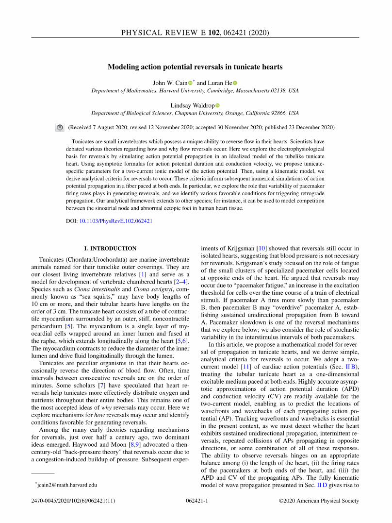
Figure 7(a) shows the results of applying this pacing proto-col in a fiber of length L = 3.0 cm with period B = 2000 ms.The asymptotic formulas (3) and (4) predict that, for this B,the steady-state values of APD, DI, and CV are 1227 ms,773 ms, and 2.665 cm/s (respectively), predicting that eachaction potential in the wave train should require 1126 msto traverse the fiber. Let t = 0 correspond to the final timeat which the the left pacemaker fires prior to the firing ofthe right pacemaker. Substituting D∗ = 773 ms into Eqs. (6)and (7), the above asymptotic approximations predict that thewavefront and waveback of the resulting action potential willarrive at the far end of the fiber at times φ(3.0) = 1126 msand β(3.0) = 1126 + 1227 = 2353 ms. Thus, a vulnerablewindow for triggering right-to-left propagation is expected tostart at t ≈ 2353 ms. These numbers are remarkably close tothose observed in numerical simulations of the PDE model,using a forward Euler solver with �t = 0.01 ms and �x =0.0025 cm. In the PDE model simulations, the steady-statevalues of APD and DI were 1223 and 777 ms, and the timerequired for the left-to-right APs to traverse the fiber was1123 ms. By firing the right pacemaker at time t = 2400 ms(see figure), a right-to-left propagating AP was generated.Despite the fact that this AP was generated very early withinthe vulnerable window, a collision with a left-to-right APstill occurred (t ≈ 2.08 s, x ≈ 2.1 cm). For this particular Band fiber length L, it is impossible to completely reverse thedirection of propagation with a single stimulus, no matter howearly in the vulnerable window such a stimulus is applied.

In order to accomplish a reversal of propagation using asingle, well-timed stimulus of the right pacemaker, we re-peated these simulations with a shorter fiber (L = 2.0 cm)and a longer B for the left pacemaker (B = 3000 ms). Theresults are shown in Fig. 7(b). The asymptotic formulas (3)and (4) predict that, for this B, the steady-state values ofAPD, DI, and CV are 1244 ms, 1756 ms, and 2.702 cm/s(respectively), suggesting that each AP in the wave trainshould require 740 ms to traverse the fiber. Substituting D∗ =1756 ms into Equations (6) and (7), this time the asymptoticapproximations predict that the wavefront and waveback of

062421-7

CAIN, HE, AND WALDROP PHYSICAL REVIEW E 102, 062421 (2020)

0

1

2

3

4

0 1 2 3

t (se

cond

s)

x (cm)

0

1

2

3

4

0 1 2

t (se

cond

s)

x (cm)

(a) (b)

FIG. 7. Space-time plots of wavefronts (dark red) and wavebacks (light blue) of action potentials in simulations of tunicate heart tissue,assuming that the left pacemaker fires periodically and the right pacemaker fires a single stimulus during the vulnerable time window. Stimuliare indicated by bold dots. (a) A collision of action potentials on the interior of the fiber. (b) Establishment of retrograde propagation via asingle, well-timed stimulus of the right pacemaker. See text for details.

the resulting action potential will arrive at the far end of thefiber at times φ(2.0) = 740 ms and β(2.0) = 740 + 1244 =1984 ms. Thus, a vulnerable window for triggering right-to-left propagation is expected to start at t ≈ 1984 ms. As before,there is excellent (less than 1% relative error) agreement be-tween the times φ(2.0) and β(2.0) predicted by asymptoticsand the times obtained by numerical simulations of the PDEmodel. By firing the right pacemaker at t = 2000 ms (i.e.,almost immediately after the predicted start of a vulnerablewindow), a right-to-left propagating AP was generated. ThisAP traversed the entire fiber, reaching the x = 0 boundary attime t = 2820 ms, shortly before the left pacemaker was dueto fire at t = 3000 ms. Because cells in the vicinity of the leftpacemaker had not recovered excitability by t = 3000 ms, aleft-to-right propagating AP was not generated.

4. Discordant alternans and conduction block

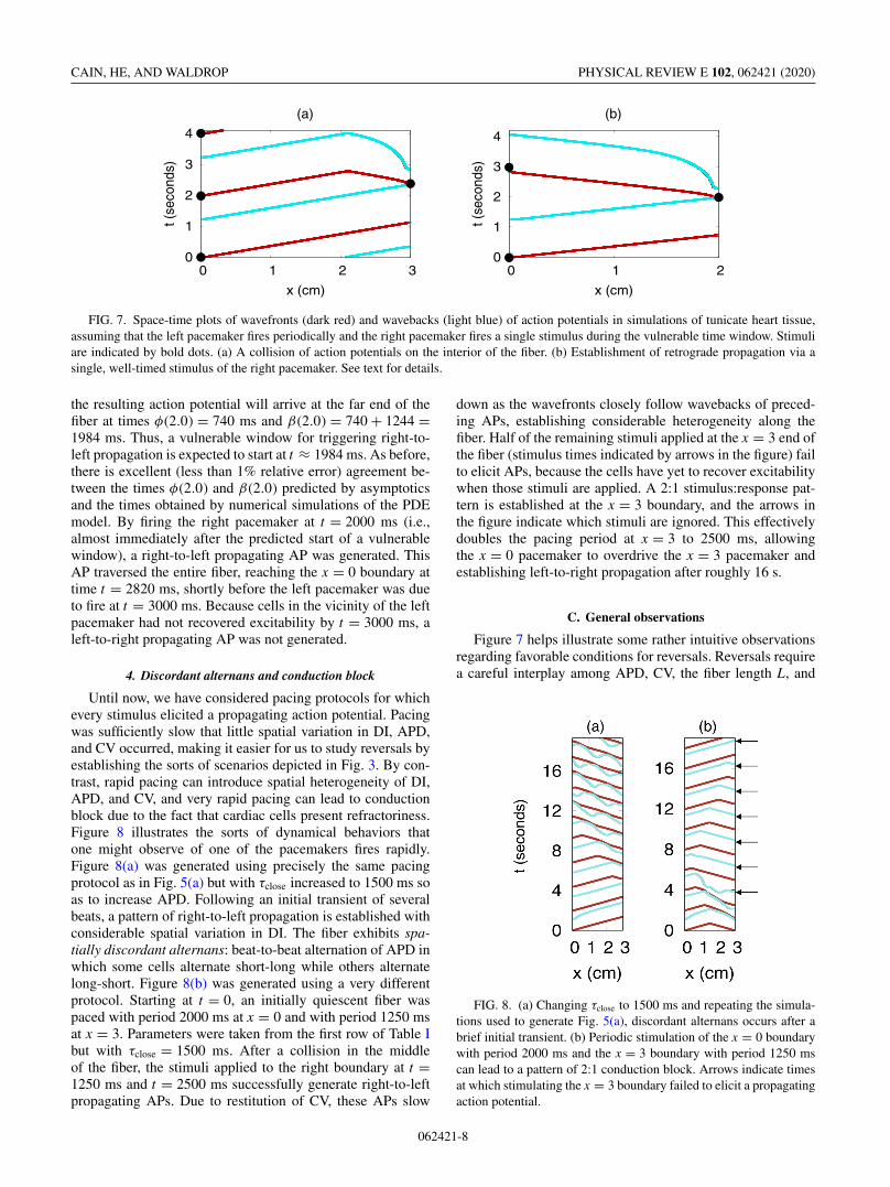
Until now, we have considered pacing protocols for whichevery stimulus elicited a propagating action potential. Pacingwas sufficiently slow that little spatial variation in DI, APD,and CV occurred, making it easier for us to study reversals byestablishing the sorts of scenarios depicted in Fig. 3. By con-trast, rapid pacing can introduce spatial heterogeneity of DI,APD, and CV, and very rapid pacing can lead to conductionblock due to the fact that cardiac cells present refractoriness.Figure 8 illustrates the sorts of dynamical behaviors thatone might observe of one of the pacemakers fires rapidly.Figure 8(a) was generated using precisely the same pacingprotocol as in Fig. 5(a) but with τclose increased to 1500 ms soas to increase APD. Following an initial transient of severalbeats, a pattern of right-to-left propagation is established withconsiderable spatial variation in DI. The fiber exhibits spa-tially discordant alternans: beat-to-beat alternation of APD inwhich some cells alternate short-long while others alternatelong-short. Figure 8(b) was generated using a very differentprotocol. Starting at t = 0, an initially quiescent fiber waspaced with period 2000 ms at x = 0 and with period 1250 msat x = 3. Parameters were taken from the first row of Table Ibut with τclose = 1500 ms. After a collision in the middleof the fiber, the stimuli applied to the right boundary at t =1250 ms and t = 2500 ms successfully generate right-to-leftpropagating APs. Due to restitution of CV, these APs slow

down as the wavefronts closely follow wavebacks of preced-ing APs, establishing considerable heterogeneity along thefiber. Half of the remaining stimuli applied at the x = 3 end ofthe fiber (stimulus times indicated by arrows in the figure) failto elicit APs, because the cells have yet to recover excitabilitywhen those stimuli are applied. A 2:1 stimulus:response pat-tern is established at the x = 3 boundary, and the arrows inthe figure indicate which stimuli are ignored. This effectivelydoubles the pacing period at x = 3 to 2500 ms, allowingthe x = 0 pacemaker to overdrive the x = 3 pacemaker andestablishing left-to-right propagation after roughly 16 s.

C. General observations

Figure 7 helps illustrate some rather intuitive observationsregarding favorable conditions for reversals. Reversals requirea careful interplay among APD, CV, the fiber length L, and

FIG. 8. (a) Changing τclose to 1500 ms and repeating the simula-tions used to generate Fig. 5(a), discordant alternans occurs after abrief initial transient. (b) Periodic stimulation of the x = 0 boundarywith period 2000 ms and the x = 3 boundary with period 1250 mscan lead to a pattern of 2:1 conduction block. Arrows indicate timesat which stimulating the x = 3 boundary failed to elicit a propagatingaction potential.

062421-8

MODELING ACTION POTENTIAL REVERSALS IN … PHYSICAL REVIEW E 102, 062421 (2020)

FIG. 9. Space-time plot of wavefronts (dark, red) and wavebacks (light, blue) of simulated APs in a fiber of length L = 3.0 cm. The x = 0end of the fiber was paced with constant period 650 ms while the x = 3 end of the fiber was paced with constant period 350 ms. (a) Steady-stateresponse using the parameters in the second row of Table I. (b) Same as in (a) but with τclose reduced to 75 ms. (c) Same as in (a) except thatκ = 10−5. (d) Same parameters as in (c), showing the initial transient response if the x = 3 pacemaker had been turned off prior to time t = 0.See text for details.

the firing rates of both pacemakers. Here are some concreteobservations:

(i) Small L tends to favor unidirectional propagation, be-cause each AP is more likely to traverse the fiber withoutcolliding with an AP propagating in the opposite direction.Large L increases the likelihood of collisions between APstraveling in opposite directions.

(ii) When two pacemakers fire with vastly different meaninterstimulus intervals, there is increased likelihood of estab-lishing unidirectional propagation from the faster pacemakertoward the slower pacemaker.

(iii) Equations (3) and (4) and the remarks in Sec. III Aelucidate the roles of the two-current model parameters in pro-moting reversals and/or collisions of APs within the interiorof the spatial domain. Figure 9(a) illustrates the steady-stateresponse obtained by simulating the two-current model in afiber of length L = 3.0 cm paced periodically at both ends(period 350 ms at x = 0 and period 650 ms at x = 3.0). Asustained pattern of right-to-left propagation is established,with an occasional collision whenever the x = 0 pacemakersupplies a stimulus during a vulnerable window (approxi-mately once every 4 s). As illustrated in Fig. 9(b), reducingτclose to 75 ms promotes additional collisions. This makessense intuitively—reducing τclose reduces APD but not CV.The reduction in APD lengthens the vulnerable time windows,enabling more stimuli at x = 0 to elicit left-to-right propaga-tion. Figure 9(c) was generated using the same parametersas Fig. 9(a), but with the diffusion coefficient κ reduced to10−5. Reduced κ has no effect on APD, but reduces CV. Byreducing CV while maintaining rapid pacing at the x = 3 endof the fiber, stimuli supplied at x = 0 cannot generate left-to-right propagating APs which make substantial progress beforebeing blocked by a right-to-left AP. Figure 9(d) illustrates the

initial transient obtained using the same parameters as Fig.9(c) but with the x = 3 pacemaker turned off prior to timet = 0. Due to the slow CV, there is a prolonged transient(5 beats) required for the x = 3 pacemaker to establish sus-tained right-to-left propagation.

Given a more physiologically detailed ionic model of thecardiac action potential, one might undertake a more com-prehensive survey of how key parameters affect likelihood ofreversals and collisions.

IV. DISCUSSION

In this article, we have proposed a model for heart rever-sals in tunicates, using previously published data to estimatemodel parameters. Using asymptotic approximations for APDand CV restitution functions [Eqs. (3) and (4)], we derivedcriteria for initiating retrograde propagation and/or trigger-ing a reversal via a single stimulus within the vulnerabletime window [Eqs. (7) and 9)]. Equipped with these resti-tution functions and reversal criteria, it is easy to identifyheart lengths L and pacing protocols that generate reversals.Because the restitution functions are derived from an ionicmodel, one may explore the roles played by various phys-iological parameters (such as τin, a time constant looselyassociated with the fast sodium current) in promoting orinhibiting reversals. Numerical simulations of gradual pace-maker variability, as illustrated in Fig. 5, produce dynamicalbehavior similar to that observed experimentally (see alsothe next paragraph). Notably, our numerical simulations alsosuggest that variability of pacemaker firing rates may elicit re-versals (Fig. 6), even if both pacemakers have the same meaninterstimulus interval. However, it is unlikely that such vari-ability alone could be the primary mechanism for reversals.

062421-9

CAIN, HE, AND WALDROP PHYSICAL REVIEW E 102, 062421 (2020)

Otherwise, our model would suggest that many collisions ofAPs might occur whenever the pacemakers are approximatelyin-phase with one another. This may lead to prolonged timewindows (tens of seconds) during which neither pacemakeris able to establish dominance, thereby preventing the heartfrom effectively pumping. It seems plausible that tunicatesexperience some hybrid of (i) gradual drift of pacemaker firingrates and (ii) stochastic heart rate variability, and that theformer is the primary contributor to reversals.

Our mathematical model captures key phenomena appear-ing in our experimentally obtained video (see the supplemen-tal material [15]). In that video, there are reversals at times00:10, 02:20, and 02:50. During the 15 s leading up to thereversal at 02:50, the period of the pacemaker driving bottom-to-top propagation is substantially longer than the period ofthe pacemaker driving top-to-bottom propagation during the15 s following the reversal. Regarding collisions, there seemto be some times (e.g., at times 02:01 and 02:04) at whichtwo advancing wavefronts clearly collide and annihilate oneanother. However, it is difficult to distinguish between actualwavefronts (those due to advancing electrical waves) and “il-lusory” wavefronts due to mechanical deformation of the heartas it relaxes after blood is pumped. For example, throughoutthe second full minute of video, top-to-bottom contraction issustained. As each downward propagating wavefront reachesthe bottom half of the heart, there is the appearance of whatlooks like a much smaller upward propagating wavefront inthe top half of the heart. We believe that this is illusory inthe sense that it is a consequence of mechanical relaxationof the heart muscle, and has nothing to do with electricalactivity. We also mention that we cannot rule out the possi-bility that the heterogeneity of the heart muscle tissue andthe three-dimensional structure of a real heart could allowtwo APs propagating in opposite directions to find conductionpathways enabling them to pass around one another, thoughwe find it highly unlikely that such behavior could occur in anormal, appropriately large heart.

While tunicates are fascinating creatures in their ownright, one might wonder about the broader importance ofunderstanding their heart behavior. Tunicates are sometimesregarded as model organisms for understanding heart de-velopment in vertebrates: as they are vertebrates’ closestinvertebrate relatives [24], it is believed that aspects of em-bryonic heart development in vertebrates can be understoodusing tunicates as a proxy [1]. There are still more compellingreasons to understand the dynamics of multiple pacemakersites. Ectopic automaticity foci in human hearts can causevarious types of arrhythmia depending on their location withinthe heart. Competition between the sinus node (the heart’snatural pacemaker, an automaticity focus located in the rightatrium) and ectopic foci can cause intermittent transitionsfrom normal rhythm to arrhythmia.

Given additional resources for experimentation, there areseveral areas of further study that we would propose. Herewe have idealized the tunicate heart as a homogeneous, one-dimensional excitable medium. A more refined model mightincorporate tissue heterogeneity and a more accurate descrip-tion of tunicate heart geometry. The two-current model ofthe membrane potential offers a major advantage in thatit lends itself to asymptotic derivation of restitution func-tions; however, it lacks the level of detail necessary forpostulating physiological bases for reversals. Asymptotic ap-proximations for APD restitution functions are available formore physiologically detailed three-current models [25–27].More detailed models of the action potential (see Ref. [28],for instance) might offer insights regarding the ionic basisfor reversals. Although asymptotic formulas for APD andCV are not available for such models, straightforward nu-merical solution of the differential equations allows one toexplore the effects of model parameters on APD and CV.Given the resources to perform additional experiments withadult tunicates, we hope to complete a careful explorationof pacemaker firing rates and heart rate variability in adulttunicates.

[1] P. Lemaire, Development 138, 2143 (2011).[2] J. Xavier-Neto, B. Davidson, M. Simoes-Costa, H. Castillo, A.

Sampaio, and A. Azambuja, in Heart Development and Regen-eration, 1st ed., edited by N. Rosenthal and R. Harvey (ElsevierScience and Technology, London, 2010), Vol. 1, pp. 3–38.

[3] A. Santhanakrishnan and L. Miller, Cell Biochem. Biophys. 61,1 (2011).

[4] B. McMahon, Comparative evolution and design in non-vertebrate cardiovascular systems, Ontogeny and Phylogenyof the Vertebrate Heart (Springer, New York, 2012),pp. 1–33.

[5] M. Kalk, Tissue and Cell 2, 99 (1970).[6] M. Anderson, J. Exp. Biol. 49, 363 (1968).[7] A. C. Heron, J. Mar. Biol. Assoc. UK 55, 959 (1975).[8] C. A. Haywood and H. P. Moon, J. Exp. Biol. 27, 14 (1950).[9] C. A. Haywood and H. P. Moon, Nature 172, 40 (1953).

[10] B. J. Krijgsman, Biol. Rev. 31, 288 (1956).[11] C. C. Mitchell and D. G. Schaeffer, Bull. Math. Biol. 65, 767

(2003).

[12] N. F. Otani, Phys. Rev. E 75, 021910 (2007).[13] M. E. Kriebel, J. General Physiol. 50, 2097 (1967).[14] M. E. Kriebel, Biol. Bull. 134, 434 (1968).[15] See Supplemental Material at http://link.aps.org/supplemental/

10.1103/PhysRevE.102.062421 for a movie of experimentallyrecorded reversals as described at the start of Sec. II and fora movie of simulated reversals as described at the start ofSec. III.

[16] L. D. Waldrop and L. A. Miller, J. Exp. Biol. 218, 2753(2015).

[17] J. W. Cain and D. G. Schaeffer, SIAM Rev. 48, 537(2006).

[18] J. W. Cain, E. G. Tolkacheva, D. G. Schaeffer, and D. J.Gauthier, Phys. Rev. E 70, 061906 (2004).

[19] Stimuli fail to elicit action potentials in cells that have notrecovered excitability following a prior excitation.

[20] For a discussion of when this is justified, see Ref. [18].[21] G. M. Hall, S. Bahar, and D. J. Gauthier, Phys. Rev. Lett. 82,

2995 (1999).

062421-10

MODELING ACTION POTENTIAL REVERSALS IN … PHYSICAL REVIEW E 102, 062421 (2020)

[22] M. Beck, C. K. R. T. Jones, D. G. Schaeffer, andM. Wechselberger, SIAM J. Appl. Dyn. Syst. 7, 1558(2008).

[23] L. A. Lipsitz, J. Mietus, G. B. Moody, and A. L. Goldberger,Circulation 81, 1803 (1990).

[24] F. Delsuc, H. Brinkmann, D. Chourrout, and H. Phillippe,Nature 439, 965 (2006).

[25] F. Fenton and A. Karma, Chaos 8, 20 (1998).[26] E. G. Tolkacheva, D. G. Schaeffer, D. J. Gauthier, and C.

Mitchell, Chaos 12, 1034 (2002).[27] D. G. Schaeffer, J. W. Cain, D. J. Gauthier, S. S. Kalb, R. A.

Oliver, E. G. Tolkacheva, W. Ying, and W. Krassowska, Bull.Math. Biol. 69, 459 (2007).

[28] C. H. Luo and Y. Rudy, Circ. Res. 74, 1071 (1994).

062421-11