Model Uncertainty, Robust Optimization and Learninglim/downloads/TutORials2006_LSS.pdf · Model Uncertainty, Robust Optimization and Learning 2 INFORMS—Pittsburgh 2006, °c 2006

INFORMS—Pittsburgh 2006 c© 2006 INFORMS | isbn 0000-0000doi 10.1287/educ.1053.0000

Model Uncertainty, Robust Optimization andLearning

Andrew E. B. Lim, J. George Shanthikumar & Z. J. Max ShenDepartment of Industrial Engineering & Operations Research, University of California at Berkeley,lim, shanthikumar, [email protected]

Abstract Classical modelling approaches in OR/MS under uncertainty assume a full probabilis-tic characterization. The learning needed to implement the policies derived from thesemodels is accomplished either through (i) classical statistical estimation procedures

or (ii) subjective Bayesian priors. When the data available for learning is limited, orthe underlying uncertainty is non-stationary, the error induced by these approachescan be significant and the effectiveness of the policies derived will be reduced. In thistutorial we discuss how we may incorporate these errors in the model (that is, modelmodel uncertainty) and use robust optimization to derive efficient policies. Differentmodels of model uncertainty will be discussed and different approaches to robust opti-

mization with and without bench-marking will be presented. Two alternative learningapproaches Objective Bayesian Learning and Operational Learning will be discussed.These approaches could be used to calibrate the models of model uncertainty and tocalibrate the optimal policies. Throughout this tutorial we will consider the classicalinventory control problem, the inventory control problem with censored demand dataand the portfolio selection problem as examples to illustrate these ideas.

Keywords Model uncertainty, Robust optimization, learning, operational statistics

1. Introduction

The majority of the early models in OR/MS are been deterministic. Specifically, modelsfor production planning, logistics and transportation have been based on the assumptionthat all variables of interest are known in advance of the implementation of the solutions.While some models, such as queueing, insurance and portfolio selections naturally call forincorporating stochasticity, it is usually assumed that the full probabilistic characterizationof these models are known in advance of the implementation of the solutions. Even when itis assumed that the parameters of a parametric stochastic model are unknown, it is assumedthat a Bayesian prior for the parameters is known (e.g., see Azoury (1985), Berger (1985),Ding, Puterman and Bisi (2002), Robert (2001)). Such an approach is often justified by theaxiomatic framework of Savage (e.g., see Savage (1972)) for decision making. Assuming thisone ends up with a model that has been fully characterized. In economics, with the initialwork of Knight (1921) and the Ellsberg paradox (Ellsberg (1961)) questions on this basicidea of full probabilistic characterization has been raised. The seminal work of Gilboa andSchmeidler (1989) provides an axiomatic framework justifying the notion of multiple fullycharacterized stochastic models for a single decision problem with a max min objective. Thissparked the basis for model uncertainty and robust optimization in the economics and financeareas (e.g. see Anderson, Hansen and Sargent (1998), (2003), Cagetti, Hansen, Sargent andWilliams (2002), Cao, Wang and Zhang (2005), Dow and Werlang (1992), Epstein (2006),Epstein and Miao (2003), Epstein and Schneider (2003), (2005a), (2005b), Epstein and Wang

1

Model Uncertainty, Robust Optimization and Learning

2 INFORMS—Pittsburgh 2006, c© 2006 INFORMS

(1994), Garlappi, Uppal and Wang (2005), Hansen and Sargent (2001), (2001), (2003)).For a recent account of the application of model uncertainty and robust optimization ineconomics and finance see the monograph by Hansen and Sargent (2006). Within the OR/MScommunity interest in deterministic robust optimization has been strong recently (e.g., seeAtamturk (2003), Atamturk and Zhang (2004), Averbakh (2000), (2001), (2004), Ben-Taland Nemirovski (1998), (1999), (2000), (2002), Bertsimas, Pachamanova and Sim (2004),Bertsimas and Sim (2004a), (2004b), (2006), El Ghaoui and Lebret (1997) and El Ghaoui,Oustry and Lebret (1998)). See Soyster (1973) for one of the earliest contribution to thisarea and the book by Kouvelis and Yu (1997) for a detailed account of the developmentsuntil the mid 90’s. However stochastic models of model uncertainty has not received asmuch attention as the others in the OR/MS literature. In this tutorial we will describethe different ideas in modelling model uncertainty, finding the solution to this model usingrobust optimization and its implementation through learning.

Consider a static or a discrete time dynamic optimization problem defined on a samplespace (Ω,F , (Fk)k∈M). Here M= 0,1,2, . . . ,m, where m is the number of decision epochs(m = 1 for a static optimization problem, m = 2 in a stochastic programming problemwith recourse, and m ≥ 2 for a discrete dynamic optimization problem). Ω is the set of allpossible outcomes of the input variables Y0 and the future values Y = Yk, k = 1,2, . . . ,mof interest for the optimization problem (such as the demand over time for different items inan inventory control problem, the arc lengths and costs in a network optimization problem,etc.). F is the sigma algebra of event in Ω and F0 is (the sigma algebra of) all possibleinformation on the input variables that may be available to the decision maker at time 0(such as the past demand or sales data for the different items in an inventory control problemor the arc lengths and costs in network optimization problem). The actual information I0

available to the decision maker is an element of F0. Though it is not required, Fn is oftenthe sigma algebra generated by the internal history of the variables Yk, k ∈M (that is,Fk = σ(Yj , j = 0,1,2, . . . , k)). It should be noted that the information that is available to thedecision maker at the beginning of period k + 1 (k ≥ 1) may not be Fk (for example, in aninventory control problem one may only have information on the sales and not the actualdemand values).

Let π1 be the decision made at the beginning of period 1 (which is adapted to an informationsubset I0 in F0). This leads to an information set that may depend on π1. Let I1(π1) be thesigma algebra generated by this information set (which satisfies I1(π1)⊂F1). Now let π2 bethe decision made at the beginning of period 2 (which is adapted to I1(π1)). In general, thepolicy π is adapted to an information filtration ((Ik(π))k∈M) which in turn is sequentiallygenerated by the policy π.

Let ψ(π,Y) be the reward obtained with policy π and Γ be the collection of all admissiblepolicies π. We are then interested in finding a policy π∗ ∈ Γ that maximizes ψ(π,Y) in somesense. One may adapt several alternative approaches to do this. All of these approaches insome way need to define a probability measure (say P ) on (Ω,F , (Fk)k∈M) given I0. Clas-sical modelling approaches in OR/MS under uncertainty assume that a full probabilisticcharacterization can be done very accurately (that is, we have perfect forecasting capa-bility when a non degenerate measure is used in our model AND that we have the capabilityto predict the future perfectly when the assumed measure is degenerate). When we dothis we hope one or both of the following is true:

THE ASSUMPTIONS

• A1: The chosen probability measure P is the true probability measure P0 or very close(in some sense) to it.


INFORMS—Pittsburgh 2006, c© 2006 INFORMS 3

• A2: The solution (optimal in some sense ) obtained with P leads to a performance thatis either optimal or close to optimal (in some sense) with respect to P0.

The learning needed to implement the policies derived from these models is accomplishedeither through (i) classical statistical estimation procedures or (ii) subjective Bayesian priors.It is not hard to see that the assumptions in many cases need not be true! When the dataavailable for learning is limited, or the underlying uncertainty is non-stationary, the errorinduced by these approaches can be significant and the effectiveness of the policy derivedwill be reduced. In this tutorial we discuss how we may incorporate these errors in the model(that is, model model uncertainty) and use robust optimization to derive efficient policies.Different models of model uncertainty will be discussed and different approaches to robust

optimization with and without bench-marking will be presented. Two alternative learningapproaches Objective Bayesian Learning and Operational Learning will be discussed. Theseapproaches could be used to calibrate the models of model uncertainty and to obtain robustoptimal policies.

Before proceeding further with this discussion we will introduce a very simple canonicalexample: The Newsvendor Inventory Problem with Demand Observed. This can be thoughtof as a sequence of n static problems. This model is almost always used as a RAT toexperiment with to test different ideas in inventory control. It will allow us to discuss theimportance of model uncertainty and the integration of optimization and estimation. Later,in Section 7 we will work out three classes of dynamic optimization problems that will serveas examples to illustrate our ideas on learning with integrated dynamic optimization andestimation and robust optimization with bench-marking.

THE INVENTORY RAT: Consider perishable item inventory control problem. Items arepurchased at c per unit and sold for s per unit. There is no salvage value and no lost salespenalty. Suppose Y1, Y2, . . . , Ym represent the demand for this item for the next m periods.We wish to find the optimal order quantities for the next m periods. Suppose we order πk

units in period k. Then the profit is

ψ(π,Y) =

m∑

k=1

sminYk, πk− cπk.

This problem allows us to illustrate the effects of separating modelling and optimizationfrom model calibration without having to bring in the consequences of cost-to-go (that is,residual) effects of current decisions at each decision epoch on future time periods. In evalu-ating the different approaches we will assume that Y1, Y2, . . . , Ym are i.i.d. with an absolutelycontinuous distribution function FY . Further, if needed we will assume that Yk is exponen-tially distributed with mean θ (that is FY (y) = 1− exp− 1

θy, y ≥ 0). Let X1,X2, . . . ,Xn

be the past demand for the last n periods. This information is contained in Y0. We will alsoassume that X1, . . . ,Xn are i.i.d samples from the same distribution as Yk.

In Section 2 we will discuss what is done now: how models are formulated, optimized andimplemented. Following a discussion on the possible errors in the current approaches inSection 2, alternative approaches to model these errors through flexible modelling will bediscussed in Section 3. Flexible modelling will be accomplished through defining a collectionof models that is very likely to contain the correct model or a close approximation of it.Hence finding a robust solution to these collection of models depends on defining a robustoptimization approach. Alternative approaches to robust optimization are discussed is Sec-tion 4. Section 5 is devoted to the calibration of flexible models using classical statistics.



Integrated learning in flexible models using (i) min-max, duality and objective Bayesianlearning and (ii) operational learning is introduced in Section 6. Detailed application of theconcepts discussed in this tutorial to dynamic inventory control and portfolio selection aregiven in Section 7.

2. Modelling, Optimization and Implementation

Almost always the abstract formulation of the model and optimization is done independentof I0 and how the model will be calibrated. Here and in the remaining of the paper we willassume that Y0 contains the past n values Xk, k = 1,2, . . . , n that will be used to calibrateY (that is, its probability measure P ).

2.A. Deterministic Modelling, Optimization and Implementation

Though this is obvious, we wish to discuss deterministic modelling here since it forms a basisfor a large body of work currently being done in robust optimization (e.g., see the specialissue of Mathematical Programming, 107, Numbers 1-2 on this topic). Let P d

ω0= Iω = ω0,

ω0 ∈ Ω be a collection of degenerate (Dirac) probability measures on (Ω,F , (Fk)k∈M). Indeterministic modelling one assumes that for some chosen ω0 ∈Ω, we have P = P d

ω0. Then

φ(π,ω0) = E[ψ(π,Y)] = ψ(π,Y(ω0)).

Given that the feasible region of π is Γ one then has the following optimization problem:

φd(ω0) = maxπ∈Γ

φ(π,ω0)

and choose a πd(ω0)∈ Γ such that

φ(πd(ω0), ω0) = φd(ω0).

To implement this policy, however, one would have to estimate Y(ω0). For example one mayassume that X1, . . . ,Xn, Y1, . . . , Ym are i.i.d. and estimate Y(ω0) by say,

Yk(ω0) = X, k = 1,2, . . . ,m,

where

X =1

n

n∑

k=1

Xk.

For some problems, the effect of variability on the final solution may be insignificant sothat such an assumption of determinism can be justified. For most real problems, however,such an assumption may be unacceptable. Often, such an assumption is made so that theresulting optimization problems are linear programs or integer linear programs so that someof the well established approaches in OR can be used to solve these optimization problems.Sometimes, even with this assumption of determinism, the solution may be hard to get. It isfair to say that the decision to assume determinism is mostly motivated by the desire to get asolution rather than to capture reality. However, with all the advances that have been madein convex optimization (e.g., see Bertsekas (2003) and Boyd and Vandenberghe (2004)) andin Stochastic Programming (e.g., see Birge and Louveaux (1997), Ruszczynski and Shapiro(2003), and van der Vlerk (2006)), it seems possible to relax this assumption and proceedto formulate stochastic models. Before we proceed to discuss stochastic modelling, we will



give the deterministic version of the inventory rat. We will later use this result in robustoptimization with bench-marking.

THE INVENTORY RAT (continued)

φd(ω0) = max

m∑

k=1

ψ(πk, Yk(ω0)) : πk ≥ 0= (s− c)

m∑

k=1

Yk(ω0)

andπd

k(ω0) = Yk(ω0), k = 1,2, . . . ,m.

Then the expected profit isφd(θ) = (s− c)mθ.

where θ = E[Yk].

To implement this policy we need to know the future demand. If we don’t, maybe we canapproximate the future demand by the observed average! Hence the implemented policywould be

πdk = X, k = 1,2, . . . ,m

with profit

ψ(Y ) =

m∑

k=1

sminYk, X− cX,

where X = 1n

∑n

k=1 Xk. Depending on when policy change is allowed, re-optimization willtake place at sometime in the future. Here and in the rest of the paper we will assume thatwe are allowed to re-optimize at the end of each period. Now depending on the belief wehave on the i.i.d assumption for the demand, we may be willing to estimate the demand forthe next period based only on the last, say, l periods. For ease of exposition we will assumethat l = n. Set Xn+j = Yj , j = 1,2, . . . ,m. Then using an updated estimate of Yk(ω0) at thebeginning of period k we get

πdk = Xk, k = 1,2, . . . ,m,

where Xk = 1n

∑n+k−1j=k Xj is the n-period moving average for k = 1,2, . . . ,m. The associated

profit is

ψ(Y ) =

m∑

k=1

sminYk, Xk− cXk.

Suppose the demand is exponentially distributed with mean θ. It is easy to verify that

limm→∞

1

mψ(Y ) = (s− c)θ− sθ(

n

n+1)n.

As n →∞ one gets an average profit of (s− c)θ − sθ exp−1. It can be verified that thisprofit can be very inferior to the optimal profit. For example, when s

c= 1.2, c = 1 and θ = 1,

the optimal profit is 0.121 while the above policy results in a profit of −0.241.

2.B. Stochastic Modelling and Optimization

For stochastic modelling, we assume a non-degenerate probability measure. That is, wedefine , given I0 a non-degenerate probability measure P on (Ω,F , (Fk)k∈M). Wanting tospecify a probability measure without any statistical assumption is indeed an idealized goal.Even if we are able to solve the resulting optimization problem, the calibration of P given



I0 will almost always require us to make some statistical assumptions regarding Y and Y0.These assumptions are often such as i.i.d., Markovian, autoregressive of some order etc. Ifthe state space of Y is finite, then we may try to solve the problem with respect to theprobabilities assigned to the different states (treating them as parameters). Even then itmay be difficult to solve the optimization problem. In such cases and in cases where furtherinformation on the distributional characteristic are known we make additional assumptionsthat allow one to fully characterize P up to some finite dimensional parameter.

2.B.1. Parametric modelling, Optimization and implementation

Suppose we have fully characterized P up to some finite dimensional parameter, say, θ.For example this may be achieved by postulating that Yk has an exponential or normaldistribution or that the transition kernel of the Markov process Y is parameterized bya finite set or the state space if finite. Let P

pθ be the corresponding probability measure

parameterized by θ. Defineφp(π, θ) = E[ψ(π,Y)].

Finding the solution to this formulation depends on one of two approaches one chooses forimplementation: Frequentist or Bayesian Approach.

Frequentist Approach Suppose we assume that the information I0 we have will allow usto estimate the parameter θ exactly. Then one solves

φp(θ) = maxπ∈Γ

φ(π, θ)

and choose a πp(θ)∈ Γ such that

φ(πp(θ), θ) = φp(θ).

To implement this policy, however, one would have to estimate θ. Suppose we use somestatistical estimator Θ(X) of θ using the data X. Then we would implement the policy

πp = πp(Θ(X)).

THE INVENTORY RAT (continued): When the demand is exponentially distributed onehas (e.g., see Liyanage and Shanthikumar (2005), Porteus (2002) and Zipkin (2000)),

φp(π, θ) = E[ψ(π,Y)] = sθ(1− exp−π

θ)− cπ,

πp(θ) = θ ln(s

c),

andφp(θ) = (s− c)θ− cθ ln(

s

c).

For an exponential distribution, the sample mean is the uniformly minimum variance unbi-ased (UMVU) estimator. Hence we will use the sample mean of the observed data to estimateθ. Then the implemented policy would be

πpk = X log(

s

c), k = 1,2, . . . ,m.

with profit

ψ(Y ) =m

∑

k=1

sminYk, X log(s

c)− cX log(

s

c),



where X = 1n

∑n

k=1 Xk. If we use the updated estimate of θ at the beginning of period k weget

πpk = Xk log(

s

c), k = 1,2, . . . ,m.

With this implementation,

ψ(Y ) =

m∑

k=1

sminYk, Xk log(s

c)− cXk log(

s

c),

and it can be easily verified that (see Liyanage and Shanthikumar 2005)

limm→∞

1

mψ(Y ) = sθ(1− (

n

n+ log( sc))n)− cθ log(

s

c).

Observe that the average profit achieved is smaller than the expected profit (s − c)θ −cθ ln( s

c). For small values of n this loss can be substantial. For example, when n = 4 and

sc

= 1.2, the percent loss over the optimal value with known θ is 22.86. (see Liyanage andShanthikumar 2005, page 343). When the demand is non-stationary, we will be forced touse a moving average or exponential smoothing to forecast the future demand. In such acase, we will need to use a small value for n.

Subjective Bayesian Approach Under the subjective Bayesian approach, given I0 oneassumes that the parameter characterizing the measure is random and postulates a dis-tribution for that parameter (Θ). Suppose, we assume that the density function of Θ isfΘ(θ), θ ∈Θ and the conditional density of Θ|X as fΘ|X(θ|X), θ ∈Θ. The objective func-tion in this case is

EΘ[φ(π,Θ)|X] =

∫

θ∈Θ

φ(π, θ)fΘ|X(θ|X)dθ .

LetπB

fΘ(X) = argmaxEΘ[φ(π,Θ)|X] : π ∈ Γ

andφB

fΘ(θ) = EX[φ(πB

fΘ(X), θ)].

THE INVENTORY RAT (continued): Often the subjective prior is chosen to be the conju-gate of the demand distribution (e.g., see Azoury 1985). When the demand is exponentiallydistributed we should choose the Gamma prior for the unknown rate, say λ = 1

θof the

exponential distribution (e.g., see Robert (2001), page 121). So let (for α, β > 0)

fΘ(θ) =(β

θ)α+1

βΓ(α)exp−

β

θ, θ ≥ 0.

Note that E[Λ] = E[ 1Θ ] = α

β. We still need to choose the parameters α and β for this prior

distribution. Straightforward algebra will reveal that

πBfΘ

(X) = (β +nX)((s

c)

1α+n − 1).

Even if the demand distribution is exponential, if the demand mean is non-stationary theBayesian estimate will converge to an incorrect parameter value. Hence we need to re-initiatethe prior distribution every now and then. Suppose we do that every n periods. Then



πBk:fΘ

(X) = (β +nXk)((s

c)

1α+n − 1), k = 1,2, . . . ,m,

with profit

ψ(Y ) =m

∑

k=1

sminYk, (β +nXk)((s

c)

1α+n − 1)− c(β +nXk)((

s

c)

1α+n − 1).

With this implementation, it can be verified that

limm→∞

1

mψ(Y ) = sθ(1− (

θ

( sc)

1α+n + θ− 1

)n exp−β

θ((

s

c)

1α+n − 1))− c(β +nθ)((

s

c)

1α+n − 1).

For bad choices of α and β the performance can be poor. The success of this policy willdepend on a lucky guess for α and β.

2.B.2 Non-Parametric modelling

Suppose we have characterized P without making any assumptions regarding the parametricform of Y. Now define

φg(π,P ) = E[ψ(π,Y)]

and solveφg(P ) = max

π∈Γφ(π,P )

and choose a πg(P )∈ Γ such that

ψ(πg(P ), P ) = φg(P ).

THE INVENTORY RAT (continued): Observe that the optimal order quantity πg(FY ) fordemand distribution FY is given by

πg(FY ) = F invY (

c

s),

where F invY is the inverse of the survival function (FY = 1− FY ) of the demand. We may

therefore use the empirical demand distribution ( ˆFY ) to obtain an estimate of the orderquantity. Let X[0] = 0 and X[r] be the r-th order statistic of X1, . . . ,Xn, r = 1,2, . . . , n.Since the demand is assumed to be continuous, we set

ˆFY (x) = 1−1

nr− 1+

x−X[r−1]

X[r] −X[r−1], X[r−1] < x≤X[r], r = 1,2, . . . , n.

Then the implemented order quantity πg based on the empirical distribution is

πg = ˆFinv

X (c

s) = X[r−1] + a(X[r] −X[r−1]),

where r ∈ 1,2, . . . , n satisfies

n(1−c

s) < r ≤ n(1−

c

s)+ 1

anda = n(1−

c

s)+ 1− r.



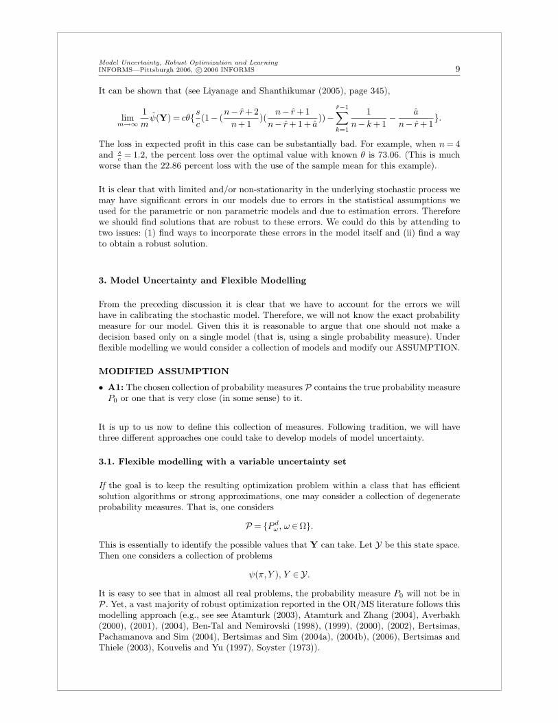
It can be shown that (see Liyanage and Shanthikumar (2005), page 345),

limm→∞

1

mψ(Y) = cθ

s

c(1− (

n− r +2

n+1)(

n− r +1

n− r +1+ a))−

r−1∑

k=1

1

n− k +1−

a

n− r +1.

The loss in expected profit in this case can be substantially bad. For example, when n = 4and s

c= 1.2, the percent loss over the optimal value with known θ is 73.06. (This is much

worse than the 22.86 percent loss with the use of the sample mean for this example).

It is clear that with limited and/or non-stationarity in the underlying stochastic process wemay have significant errors in our models due to errors in the statistical assumptions weused for the parametric or non parametric models and due to estimation errors. Thereforewe should find solutions that are robust to these errors. We could do this by attending totwo issues: (1) find ways to incorporate these errors in the model itself and (ii) find a wayto obtain a robust solution.

3. Model Uncertainty and Flexible Modelling

From the preceding discussion it is clear that we have to account for the errors we willhave in calibrating the stochastic model. Therefore, we will not know the exact probabilitymeasure for our model. Given this it is reasonable to argue that one should not make adecision based only on a single model (that is, using a single probability measure). Underflexible modelling we would consider a collection of models and modify our ASSUMPTION.

MODIFIED ASSUMPTION

• A1: The chosen collection of probability measures P contains the true probability measureP0 or one that is very close (in some sense) to it.

It is up to us now to define this collection of measures. Following tradition, we will havethree different approaches one could take to develop models of model uncertainty.

3.1. Flexible modelling with a variable uncertainty set

If the goal is to keep the resulting optimization problem within a class that has efficientsolution algorithms or strong approximations, one may consider a collection of degenerateprobability measures. That is, one considers

P = P dω , ω ∈Ω.

This is essentially to identify the possible values that Y can take. Let Y be this state space.Then one considers a collection of problems

ψ(π,Y ), Y ∈Y.

It is easy to see that in almost all real problems, the probability measure P0 will not be inP. Yet, a vast majority of robust optimization reported in the OR/MS literature follows thismodelling approach (e.g., see see Atamturk (2003), Atamturk and Zhang (2004), Averbakh(2000), (2001), (2004), Ben-Tal and Nemirovski (1998), (1999), (2000), (2002), Bertsimas,Pachamanova and Sim (2004), Bertsimas and Sim (2004a), (2004b), (2006), Bertsimas andThiele (2003), Kouvelis and Yu (1997), Soyster (1973)).



3.2. Flexible modelling with a parametric uncertainty set

Suppose our statistical assumptions are valid and the only unknown are the true parametervalues. Then the collection of measures we consider could be

P = P pθ , θ ∈Θ,

for some set Θ of parameter values. Then one considers a collection of problems

φp(π, θ), θ ∈Θ.

This appears to be a very promising way to formulate and solve real problems. Applicationof this approach to portfolio optimization is discussed in Lim, Shanthikumar and Watewai(2005), (2006b).

3.3. Flexible modelling with a non-parametric uncertainty set

For flexible modelling with a non-parametric uncertainty set, we first identify a nominalmodel (or probability measure, say P ). Then the collection of models are chosen to be aclosed ball around this nominal model. Let d(P, P ) be some distance measure between P

and P . If the measures are fully characterized by a density (or distribution) function, thedistance will be defined with respect to the density (or distribution) functions. The collectionof models thus considered will be

P = P : d(P, P )≤ α,

where α is the minimum deviation that we believe is needed to assure that the true proba-bility measure P0 is in P. Some of the distance measures commonly used are listed below.

Distance Measures for Density Functions

We will specify the different types of distances for the density functions of continuous randomvariables. Analogous distances can be defined for discrete random variables as well.

Kullback-Leibler Divergence (Relative Entropy)

dKL(f, f) =

∫

x

f(x) log(f(x)

f(x))dx.

It is easy to verify that dKL takes values in [0,∞] and is convex in f . However it is not ametric (it is not symmetric in (f, f) and does not satisfy the triangle inequality). One veryuseful property of dKL is that it is sum separable for product measures. This comes in veryhandy in dynamic optimization with model uncertainty.

Hellinger Distance

dH(f, f) =

√

1

2[

∫

x

(√

f(x)−

√

f(x))2dx]12 .

Hellinger distance as defined above is a metric that takes a value in [0,1]. One useful propertyof this metric in dynamic optimization is that the Hellinger affinity (1 − d2

H) is productseparable for product measures.

Chi-Squared Distance



dCS(f, f) =

∫

x

(f(x)− f(x))2

f(x)dx.

Discrepancy Measure

dD(f, f) = sup|

∫ b

a

(f(x)− f(x))dx| : a < b.

Total Variation Distance

dTV (f, f) =1

2sup

∫

x

h(x)(f(x)− f(x))dx : |h(x)| ≤ 1.

Wasserstein (Kantorovich) Metric

dW (f, f) = sup

∫

x

h(x)(f(x)− f(x))dx : |h(x)−h(y)| ≤ |x− y|.

Distance Measures for Cumulative Distribution Functions

Kolmogorov (Uniform) Metric

dK(F, F ) = sup|F (x)− F (x)| : x∈R.

Levy (Prokhorov) Metric

dL(F, F ) = infh : F (x−h)−h≤ F (x)≤ F (x+h)+h;h > 0;x∈R.


dW (F, F ) =

∫

x

|F (x)− F (x)|dx.

Distance Measures for Measures

Kullback-Leibler Divergence (Relative Entropy)

dKL(P, P ) =

∫

Ω

log(dP

dP)dP.

Prokhorov Metric

Suppose Ω is a metric space with metric d. Let B be the set of all Borel sets of Ω and forany h > 0 define Bh = x : infy∈B d(x, y)≤ h for any B ∈B. Then

dP (P, P ) = infh : |P (B)≤ P (Bh)+h;h > 0;B ∈B.



Discrepancy Measure

Suppose Ω is a metric space with metric d. Let Bc be the collection of all closed balls in Ω.

dD(P, P ) = sup|P (B)− P (B))| : B ∈Bc.

Total Variation Distance

dTV (P, P ) = sup|P (A)− P (A)| : A⊂Ω.


Suppose Ω is a metric space with metric d.

dW (P, P ) = sup

∫

Ω

h(ω)(P (dω)− P (dω)) : |h(x)−h(y)| ≤ d(x, y), x, y ∈Ω.

The majority of the flexible modelling in finance is done using uncertainty sets for mea-sures (e.g., see Hansen and Sargent (2006) and the references in there). Application of thisapproach to dynamic programming is given in Iyengar (2005) and in revenue managementin Lim and Shanthikumar (2004) and Lim, Shanthikumar and Watewai (2006a).

4 Robust Optimization

Now that we have a collection of models, we need to decide how to find a solution for thesemodels such that the solution is indeed a very good solution for the true model. For this weassume that our robust optimization will give such a good solution.

MODIFIED ASSUMPTION

• A2: The robust solution (optimal in some sense ) obtained with the collection of measuresP leads to a performance that is either optimal or close to optimal (in some sense) withrespect to P0.

4.1. Max-min objective

The most commonly used approach to finding a (so-called) robust solution for the given setof models is to find the best solution to the worst model among the collection of models.The optimization problem is

φr = maxπ∈Γ

minP∈P

φ(π,P ).

and the solution sought is:πr = argmax

π∈ΓminP∈P

φ(π,P ).

If the true model is the worst one, then this solution will be nice and dandy. However, if thetrue model is the best one or something close to it, this solution could be very bad (thatis, the solution need not be robust to model error at all!). As we will soon see, this can be



the case. However, this form of (so called) robust optimization is still very popular, sincethe resulting optimization tends to preserve the algorithmic complexity very close to that ofthe original single model case. However, if we really want a robust solution, its performanceneeds to be compared to what could have been the best for every model in the collection.This idea of bench-marking will be discussed later. Let us now look at the inventory example:

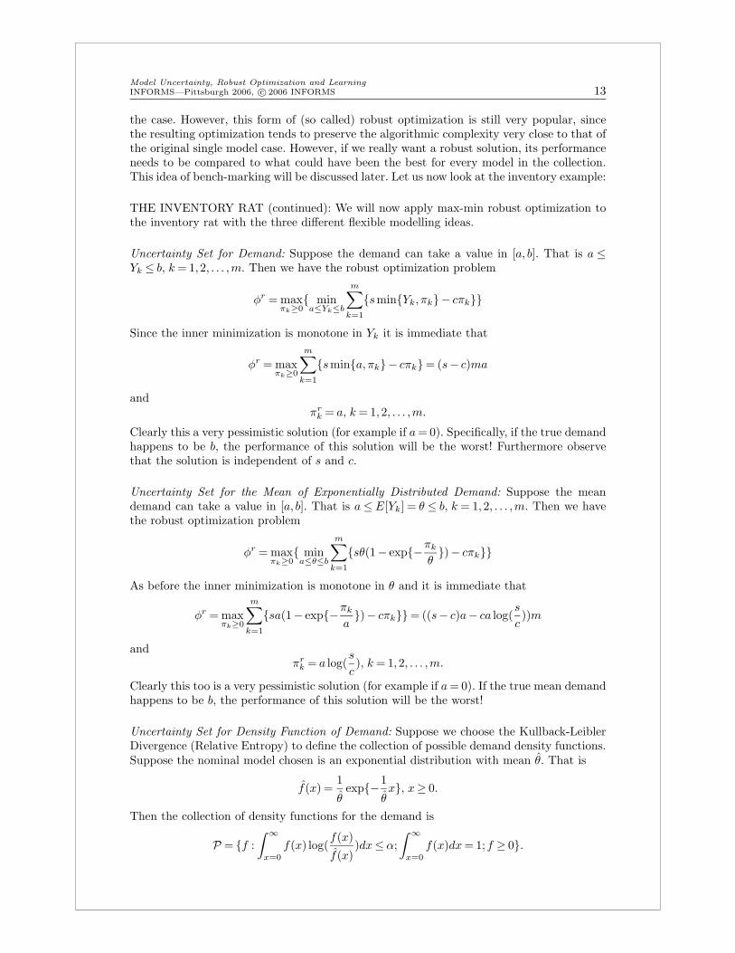
THE INVENTORY RAT (continued): We will now apply max-min robust optimization tothe inventory rat with the three different flexible modelling ideas.

Uncertainty Set for Demand: Suppose the demand can take a value in [a, b]. That is a ≤Yk ≤ b, k = 1,2, . . . ,m. Then we have the robust optimization problem

φr = maxπk≥0

mina≤Yk≤b

m∑

k=1

sminYk, πk− cπk

Since the inner minimization is monotone in Yk it is immediate that

φr = maxπk≥0

m∑

k=1

smina,πk− cπk= (s− c)ma

andπr

k = a, k = 1,2, . . . ,m.

Clearly this a very pessimistic solution (for example if a = 0). Specifically, if the true demandhappens to be b, the performance of this solution will be the worst! Furthermore observethat the solution is independent of s and c.

Uncertainty Set for the Mean of Exponentially Distributed Demand: Suppose the meandemand can take a value in [a, b]. That is a ≤ E[Yk] = θ ≤ b, k = 1,2, . . . ,m. Then we havethe robust optimization problem

φr = maxπk≥0

mina≤θ≤b

m∑

k=1

sθ(1− exp−πk

θ)− cπk

As before the inner minimization is monotone in θ and it is immediate that

φr = maxπk≥0

m∑

k=1

sa(1− exp−πk

a)− cπk= ((s− c)a− ca log(

s

c))m

andπr

k = a log(s

c), k = 1,2, . . . ,m.

Clearly this too is a very pessimistic solution (for example if a = 0). If the true mean demandhappens to be b, the performance of this solution will be the worst!

Uncertainty Set for Density Function of Demand: Suppose we choose the Kullback-LeiblerDivergence (Relative Entropy) to define the collection of possible demand density functions.Suppose the nominal model chosen is an exponential distribution with mean θ. That is

f(x) =1

θexp−

1

θx, x≥ 0.

Then the collection of density functions for the demand is

P = f :

∫ ∞

x=0

f(x) log(f(x)

f(x))dx≤ α;

∫ ∞

x=0

f(x)dx = 1;f ≥ 0.



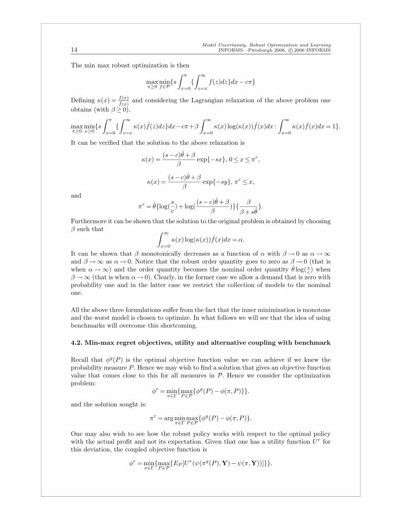
The min max robust optimization is then

maxπ≥0

minf∈P

s

∫ π

x=0

∫ ∞

z=x

f(z)dzdx− cπ

Defining κ(x) = f(x)

f(x)and considering the Lagrangian relaxation of the above problem one

obtains (with β ≥ 0),

maxπ≥0

minκ≥0

s

∫ π

x=0

∫ ∞

z=x

κ(x)f(z)dzdx−cπ+β

∫ ∞

x=0

κ(x) log(κ(x))f(x)dx :

∫ ∞

x=0

κ(x)f(x)dx = 1.

It can be verified that the solution to the above relaxation is

κ(x) =(s− c)θ +β

βexp−sx, 0≤ x≤ πr,

κ(x) =(s− c)θ +β

βexp−sy, πr ≤ x,

and

πr = θlog(s

c)+ log(

(s− c)θ +β

β)

β

β + sθ.

Furthermore it can be shown that the solution to the original problem is obtained by choosingβ such that

∫ ∞

x=0

κ(x) log(κ(x))f(x)dx = α.

It can be shown that β monotonically decreases as a function of α with β → 0 as α →∞and β →∞ as α → 0. Notice that the robust order quantity goes to zero as β → 0 (that iswhen α →∞) and the order quantity becomes the nominal order quantity θ log( s

c) when

β →∞ (that is when α→ 0). Clearly, in the former case we allow a demand that is zero withprobability one and in the latter case we restrict the collection of models to the nominalone.

All the above three formulations suffer from the fact that the inner minimization is monotoneand the worst model is chosen to optimize. In what follows we will see that the idea of usingbenchmarks will overcome this shortcoming.

4.2. Min-max regret objectives, utility and alternative coupling with benchmark

Recall that φg(P ) is the optimal objective function value we can achieve if we knew theprobability measure P . Hence we may wish to find a solution that gives an objective functionvalue that comes close to this for all measures in P. Hence we consider the optimizationproblem:

φr = minπ∈Γ

maxP∈P

φg(P )−φ(π,P ).

and the solution sought is:

πr = argminπ∈Γ

maxP∈P

φg(P )−φ(π,P ).

One may also wish to see how the robust policy works with respect to the optimal policywith the actual profit and not its expectation. Given that one has a utility function Ur forthis deviation, the coupled objective function is

φr = minπ∈Γ

maxP∈P

EP [Ur(ψ(πg(P ),Y)−ψ(π,Y))].




πr = argminπ∈Γ

maxP∈P

EP [Ur(ψ(πg(P ),Y)−ψ(π,Y))].

THE INVENTORY RAT (continued): Observe that clairvoyant ordering will result in aprofit of (s − c)Y . Hence if we order π units, the regret is (s − c)Y − sminπ,Y − cπ= smaxY −π,0− c(Y −π). Hence we wish to solve

min maxa≤Y ≤b

smaxY −π,0− c(Y −π)

The optimal solution is

πr = a+(b− 1)(s− c

s).

Unlike in the min-max robust optimization, here the order quantity depends on s and c.

4.3. Max-min competitive ratio objective with alternative coupling with bench-mark

Suppose φg(P )≥ 0 for all P ∈P. Then instead of looking at the difference in the objectivefunction values, we may wish to look at the ratios (and find a solution that achieves a ratioclose to one for all P ). Hence we consider the optimization problem:

φr = minπ∈Γ

maxP∈P

φ(π,P )

φg(P ).


πr = argminπ∈Γ

maxP∈P

φ(π,P )

φg(P ).

One may also wish to see how the robust policy works with respect to the optimal policywith the actual profit and not its expectation. Suppose ψ(πg(P ),Y) ≥ 0. Given that onehas a utility function Ur for this deviation, the coupled objective function is

φr = minπ∈Γ

maxP∈P

EP [Ur(ψ(π,Y)

ψ(πg(P ),Y)))].


πr = argminπ∈Γ

maxP∈P

EP [Ur(ψ(π,Y)

ψ(πg(P ),Y)))].

5. Classical Statistics and Flexible Modelling

We will now discuss how classical statistics can be used to characterize model uncertaintyof different types. To do this, first we have to postulate a statical model for X,Y. Supposethe extended measure for this is P e (note that, then P = P e|I0).

5.1 Predictive Regions and Variable Uncertainty Set

Let SY be the state space of Y. Now choose a predictive region Y(X)⊂SY for Y such that

P eY ∈Y(X)= 1−α,



for some appropriately chosen value of α (0 < α < 1). Then we could choose

Y = Y(X)|I0.

THE INVENTORY RAT (continued): Suppose X1,X2, . . . ,Xn, Y are i.i.d. exponentialrandom variables with mean θ. Let χ2

k be a Chi-squared random variable with k degrees offreedom and Fr,s be an F -random variable with (r, s) degrees of freedom. Then,

2n

θX =d χ2

2n

and2

θY =d χ2

2

ThereforeY

X=d F2,2n

andPf2,2n,1−α

2X ≤ Y ≤ f2,2n, α

2X= 1−α,

wherePf2,2n,β ≤ F2,2n= β,β ≥ 0.

A (1−α)100% predictive interval for Y is (f2,2n,1−α2X, f2,2n, α

2X). Hence with a min-max

objective, the robust solution is (see Section 4.1)

πr = f2,2n,1−α2X.

Observe that this implementation is independent of s and c. Alternatively, one may use aone sided predictive interval (f2,2n,1−αX, ∞). Then

πr = f2,2n,1−αX.

This too is independent of s and c. Therefore there is no guarantee that this solution willbe robust to model uncertainty! Suppose we choose an α such that

1−α = P((s

c)

11+n − 1)n≤ F2,2n.

Thenπr = ((

s

c)

11+n − 1)nX.

Later in operational learning we will find that this is indeed the optimal order quantitywhen θ is unknown. It is thus conceivable that a good policy could be obtained using adeterministic robust optimization provided we have stable demand and sufficient data totest various α. If that is the case, then retrospective optimization using the past data wouldhave yielded a very good solution anyway! The issue in this method of using min-max robustoptimization is that the solution can be sensitive to the choice α and that a good value forit cannot be chosen a priori. Hence we need a robust optimization technique that is robustwith respect to the choice of α.

5.2 Confidence Regions and Parameter Uncertainty Set

Let t(X) be an estimator of θ. Now choose a region T (θ) such that

P et(X)∈ T (θ)= 1−α,



for some appropriately chosen value of α (0 < α < 1). Now define

Θ(X) = θ : t(X)∈ T (θ).

Then we could chooseΘ = Θ(X)|I0.

THE INVENTORY RAT (continued): Suppose X1,X2, . . . ,Xn, Y are i.i.d. exponentialrandom variables with mean θ. Observing that

2n

θX =d χ2

2n,

it is immediate that

P2nX

χ22n, α

2

≤ θ ≤2nX

χ22n,1−α

2

= 1−α,

wherePχ2

2n,β ≤ χ22n= β,β ≥ 0.

A (1−α) 100 % confidence interval for θ is 2nXχ2

2n, α2

, 2nXχ2

2n,1− α2

). Hence with a min-max objective,

the robust solution is (see Section 4.1)

πr =2nX

χ22n, α

2

.

Observe that this implementation is independent of s and c. Alternatively, one may use aone sided predictive interval ( 2nX

χ22n,α

, ∞). Then

πr =2nX

χ22n,α

.

This too is independent of s and c.

6 Learning

Outside of Bayesian learning, the two popular techniques used for learning in decision makingare: (i) Reinforcement Learning (e.g., see Sutton and Barto (1998)) and (ii) StatisticalLearning (e.g., see Vapnik (2000)). Applying either one of these approaches to the inventoryrat problem results in a solution, that is the same as in the non-parametric model discussedin Section 2.B.2 (see Jain, Lim and Shanthikumar (2006)) which we already know can resultin poor results. We will not discuss these two approaches here.

6.1 Max-min, Duality and Objective Bayesian Learning

In this section we will pursue the max-min bench-marking approach discussed earlier as alearning tool. Specifically, we will consider the dual problem, which can then be seen as aform of the objective Bayesian approach (see Berger (1985), Robert (2001)).

In a dynamic optimization scenario, it is the recognition that the implemented policy πk attime k is a function of the past data X that motivates the need to incorporate learning inthe optimization itself. Hence in integrated learning and optimization, the focus is

maxπ

Eeθ [φ(π(X), θ)],



where the expectation over X is taken with respect to the probability measure P eθ .

This is indeed the focus of Decision Theory (Wald (1950)), where minimization of a lossfunction is the objective. Naturally one could define −φ as the risk function and applythe existing decision theory approaches to solve the above problem. It has already beenrecognized in decision theory that without further characterization of π one may not be ableto solve the above problem (e.g., see Berger (1985), Robert (1994)). Otherwise one couldconclude that πp(θ) is the optimal solution. Hence one abides by the notion of an efficient

policy π defined below:

Definition: A policy π0 is efficient if there does not exist a policy π such that

Eeθ [φ(π(X), θ)]≥Ee

θ [φ(π0(X), θ)],∀θ,

with strict inequality holding for some values of θ.

Observe that π0 = πp(θ0) for almost any θ0 will be an efficient solution. Indeed it is wellknown that any Bayesian solution πB(fΘ), if unique, is an efficient solution. Thus one mayhave an unlimited number of efficient policies and the idea of an efficient solution does notprovide an approach to identifying a suitable policy. While it is necessary for a solution tobe efficient, it is not sufficient (unless it is optimal).

Definition: A policy π0 is optimal, if

Eeθ [φ(π0(X), θ)]≥Ee

θ [φ(π(X), θ)],∀θ,

for all π.

It is very unlikely that such a solution can be obtained without further restriction on π forreal stochastic optimization problems. Consequently, in decision theory, one follows one ofthe two approaches. One that is commonly used in the OR/MS literature is to assume a priordistribution for the unknown parameter(s) (see Section 2.B.1). This eliminates any modeluncertainty. However this leaves one to have to find this prior distribution during implemen-tation. This task may not be well defined in practice (e.g., see Kass and Wasserman (1996)).To overcome this there has been considerable work done on developing non-informative pri-ors (e.g., see Kass and Wasserman (1996)). The relationship of this approach to what wewill do in the next two sections will be discussed later. The second approach in decisiontheory is min-maxity. In our setting, it is

maxπ

minθ

Eeθ [φ(π(X), θ)].

Unfortunately though, in almost all applications in OR/MS, EeX

[φ(π(X), θ)] will be mono-tone in θ. For example, in the inventory problem, the minimum will be attained at θ = 0. Ingeneral, suppose the minimum occurs at θ = θ0. In such a case, the optimal solution for theabove formulation is πp(θ0). Hence it is unlikely that a direct application of the min-maxapproach of decision theory to the objective function of interest in OR/MS will be appro-priate. Therefore we will apply this approach using objectives with benchmark (see Sections4.2 and 4.3 and also Lim, Shanthikumar and Shen (2006b)). In this section, we will considerthe relative performance

η(π, θ) =φ(π(X), θ)

φp(θ).



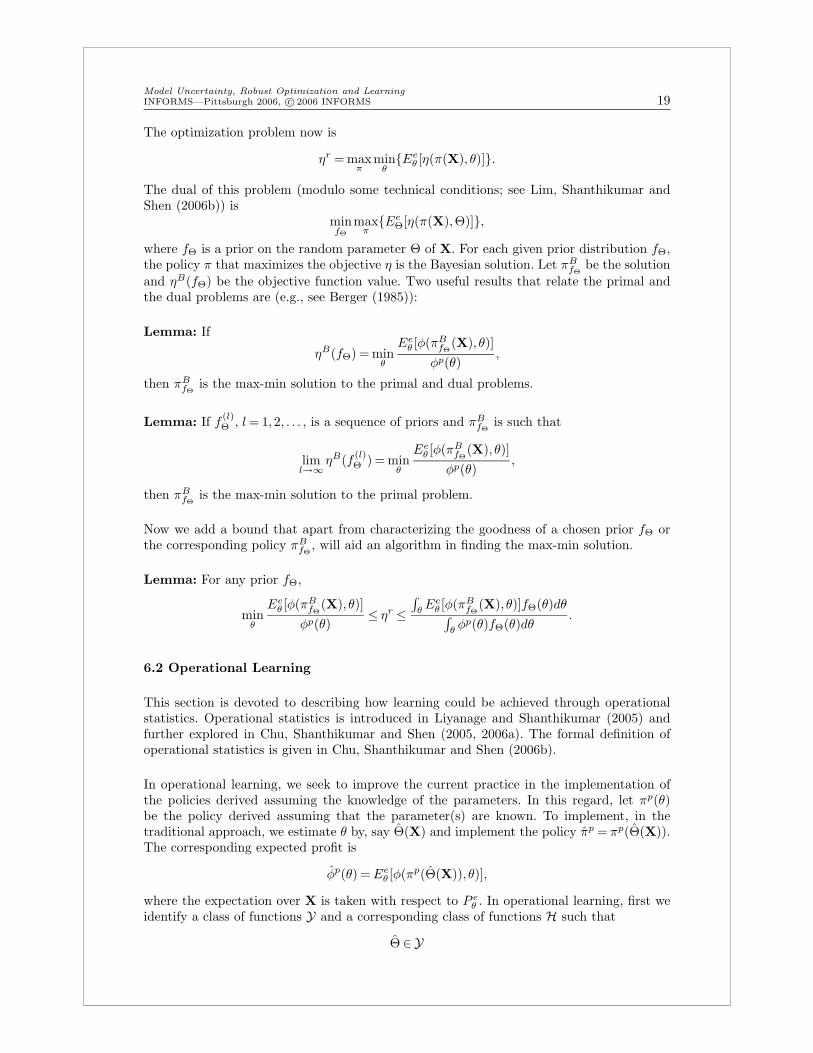
The optimization problem now is

ηr = maxπ

minθ

Eeθ [η(π(X), θ)].

The dual of this problem (modulo some technical conditions; see Lim, Shanthikumar andShen (2006b)) is

minfΘ

maxπ

EeΘ[η(π(X),Θ)],

where fΘ is a prior on the random parameter Θ of X. For each given prior distribution fΘ,the policy π that maximizes the objective η is the Bayesian solution. Let πB

fΘbe the solution

and ηB(fΘ) be the objective function value. Two useful results that relate the primal andthe dual problems are (e.g., see Berger (1985)):

Lemma: If

ηB(fΘ) = minθ

Eeθ [φ(πB

fΘ(X), θ)]

φp(θ),

then πBfΘ

is the max-min solution to the primal and dual problems.

Lemma: If f(l)Θ , l = 1,2, . . . , is a sequence of priors and πB

fΘis such that

liml→∞

ηB(f(l)Θ ) = min

θ

Eeθ [φ(πB

fΘ(X), θ)]

φp(θ),

then πBfΘ

is the max-min solution to the primal problem.

Now we add a bound that apart from characterizing the goodness of a chosen prior fΘ orthe corresponding policy πB

fΘ, will aid an algorithm in finding the max-min solution.

Lemma: For any prior fΘ,

minθ

Eeθ [φ(πB

fΘ(X), θ)]

φp(θ)≤ ηr ≤

∫

θEe

θ [φ(πBfΘ

(X), θ)]fΘ(θ)dθ∫

θφp(θ)fΘ(θ)dθ

.

6.2 Operational Learning

This section is devoted to describing how learning could be achieved through operationalstatistics. Operational statistics is introduced in Liyanage and Shanthikumar (2005) andfurther explored in Chu, Shanthikumar and Shen (2005, 2006a). The formal definition ofoperational statistics is given in Chu, Shanthikumar and Shen (2006b).

In operational learning, we seek to improve the current practice in the implementation ofthe policies derived assuming the knowledge of the parameters. In this regard, let πp(θ)be the policy derived assuming that the parameter(s) are known. To implement, in thetraditional approach, we estimate θ by, say Θ(X) and implement the policy πp = πp(Θ(X)).The corresponding expected profit is

φp(θ) = Eeθ [φ(πp(Θ(X)), θ)],

where the expectation over X is taken with respect to P eθ . In operational learning, first we

identify a class of functions Y and a corresponding class of functions H such that

Θ∈Y



andπp Θ∈H.

The second step is to choose a representative parameter value, say θ0 and solve

maxπ∈H

Eeθ0

[φ(π(X), θ0)]

subject toEe

θ [φ(π(X), θ)]≥ φp(θ),∀θ

First note that since πp Θ ∈ H, we are guaranteed that a solution exists for the aboveoptimization problem. Second note that the selection of θ0 is not critical. For it may happenthat the selection of H is such that the solution obtained is independent of θ0 (as we will seein the inventory examples). Alternatively, we may indeed use a prior fΘ on θ and reformulatethe problem as,

maxπ∈H

∫

θ

Eeθ [φ(π(X), θ)]fΘ(θ)dθ

subject toEe

θ [φ(π(X), θ)]≥ φp(θ),∀θ

It is also conceivable that alternative forms of robust optimization may be defined.

THE INVENTORY RAT (continued): Recall that πp(θ) = θ log( sc) and Θ(X) = X. So we

could choose H to be the class of order one homogenous functions. Note that

H1 = π :Rn+ →R+;π(αx) = απ(x);α≥ 0;x∈Rn

+.

is the class of non-negative order-one-homogeneous functions. Furthermore, observe that ψ isa homogeneous-order-one function (that is, ψ(αx,αY ) = αψ(x,Y )). Let Z be an exponentialr.v. with mean 1. Then Y =d θZ, and one finds that φ too is a homogeneous order onefunction (that is, φ(αx,αθ) = αφ(x, θ)).

Now suppose we restrict the class of operational statistics π to homogeneous-order-onefunctions. That is, for some chosen θ0, we consider the optimization problem:

maxπ∈H1

Eeθ0

[φ(π(X), θ0)].

subject toEe

θ [φ(π(X), θ)]≥ φp(θ),∀θ.

Let Z1,Z2, . . . ,Zn be i.i.d exponential r.v.s with mean 1 and Z = (Z1,Z2, . . . ,Zm). Then

X =d θZ.

Utilizing the property that φ,π and φp are all homogeneous order-one functions, we get

Eeθ [φ(π(X), θ)] = θEe

Z[φ(π(Z),1)]

and φp(θ) = θφp(1). Hence we can drop the constraints and consider

maxπ∈H1

EeZ[φ(π(Z),1)].

Let V (with |V|=∑m

k=1 Vk = 1) and the dependent random variable R be defined such that

fR|V(r|v) =1

rn+1

1

(n− 1)!exp−

1

r, r ≥ 0,



andfv(v) = (n− 1)!, |v|= 1; v ∈Rn

+.

Then

Z =d 1

RV.

Therefore

EZ[φ(π(Z),1)] = EV[ER[φ(π(V

R),1)|V]].

Since we assumed π to be a homogeneous-order-one function, we get

EV[ER[φ(π(Z

R),1)|V]] = EV[ER[

1

Rφ(π(V),R)]|V]].

Hence all we need to find the optimal operational statistics is to find

πos(v) = argmaxER[1

Rφ(π,R)|V = v] : π ≥ 0, v ∈Rn

+; |v|= 1.

Then the optimal homogenous order one operational statistic is (with |x|=∑n

k=1 xk),

πos(x) = |x|πos(x

|x|), x∈Rn

+.

After some algebra one finds that (see Liyanage and Shanthikumar (2005) and Chu, Shan-thikumar and Shen (2005)):

πos(x) = ((s

c)

11+n − 1)

n∑

k=1

xk

andφos(θ) = Eθ[φ(πos(X), θ)] = θ[c

s

c− 1− (n+1)((

s

c)

11+n − 1)].

This policy compared to the classical approach improves the expected profit by 4.96% forn = 4 and s

c= 1.2 (see page 344 of Liyanage and Shanthikumar (2005)).

7. Examples

7.1 Inventory Control with Observable Demand

Consider an inventory control problem with instantaneous replenishment, backlogging andfinite planning horizon. Define the following input variables:

• m - number of periods in the planning horizon• c - purchase price per unit• s - selling price per unit• Y1, Y2, . . . , Ym - demand for the next m periods• b - backlogging cost per unit per period• h - inventory carrying cost per unit per period

At the end of period m all remaining inventory (if any) is salvaged (at a salvage value ofc per unit). If at the end of period m orders are backlogged then all orders are met at thebeginning of period m+1. Let πk (πk ≥ 0) be the order quantity at the beginning of periodk (k = 1,2, . . . ,m). Then the total profit for the m periods is



ψ(π,Y) =

m∑

k=1

−cπk + smax−Wk−1,0+Yk −max−Wk,0

+ cmaxWm,0+(s− c)max−Wm,0−

m∑

k=1

hmaxWk,0+ bmax−Wk,0,

(0)

where W0 = 0 andWk = Wk−1 +πk −Yk, k = 1,2, . . . ,m.

Simple algebra reveals that,

ψ(π,Y) =

m∑

k=1

ψk(πk, Yk),

where

ψk(πk, Yk) = (s− c− b)Yk +(b+h)minWk−1 +πk, Yk−h(Wk−1 +πk), k = 1,2, . . . ,m.

Given Ik =Fk, we wish to find the optimal order quantity π∗k for period k (k = 1, . . . ,m).

First let us see what we can do if we are clairvoyant. Here we will assume that all the futuredemand is known. It is not hard to see that

πdk(ω0) = Yk(ω0), k = 1,2, . . . ,m,

and

φd(ω0) = (s− c)m

∑

k=1

Yk(ω0).

If we can implement this, then the profit experienced is ψ(Y) = (s − c)∑m

k=1 Yk and the

expected profit is E[ψ(Y)] = (s− c)mθ.

Suppose we assume that the future demand Y1, Y2, . . . , Ym for the next m periods given I0

are i.i.d. with exponential density function with mean θ (that is fY (y) = 1θexp− 1

θy, y ≥ 0).

Let

φk(q, θ) = E[(b+h)minq,Yk−hq] = (b+h)θ(1− exp−q

θ)−hq, k = 1,2, . . . ,m.

Then

q∗(θ) = argmaxφk(q, θ)= θ log(b+h

h).

It is then clear thatπk(θ) = q∗(θ)−Wk−1, k = 1,2, . . . ,m,

and

φ(θ) = (s− c)mθ−hmθ log(b+h

h).

If we use X as an estimate for the θ for implementing this policy, we get

ψ(Y) = (s− c− b)m

∑

k=1

Yk +(b+h)m

∑

k=1

minX log(b+h

h), Yk−h

m∑

k=1

X log(b+h

h),



and an a priori expected profit of

Ee[1

mψ(Y)] = (s− c)θ− bθ(

n

n+ log( b+hh

))n −hθ((

n

n+ log( b+hh

))n + log(

b+h

h)− 1).

However, if we continue to update the estimate we have

πk = maxXk log(b+h

h)−Wk−1,0, k = 1,2, . . . ,m,

and

limm→∞

ψ(Y) = Ee[1

mψ(Y)]

We will now apply operational learning to this problem (for details of this analysis seeLim, Shanthikumar and Shen (2006a)). Specifically let H1 be the collection of order-one-homogeneous functions. Then, in operational learning we are interested in

maxπk∈H1

m∑

k=1

Eeθ [φk(πk, θ)],

whereφk(πk, θ) = (b+h)E[minWk−1 +πk, Yk]−hE[(Wk−1 +πk)],

W0 = 0 andWk = Wk−1 +πk −Yk, k = 1,2, . . . ,m.

First we will consider the last period. Let Y1 be an empty vector and

Yk = (Y1, . . . , Yk−1), k = 2, . . . ,m.

Define the random vector Vm (|Vm|= 1) and the dependent random variable Rm such that(see Section 6.2)

Vm

Rm

=d (X,Ym).

Now let

πm(z) = argmaxERm[φm(q,Rm)

Rm

|Vm = z] : q ≥ 0,z∈Rn+m−1+ , |z|= 1,

andπm(x) = |x|ym(

x

|x|),x∈Rn+m−1

+ .

Defineπm(X,Ym,w) = maxym(X,Ym),w−Ym−1.

andφ∗

m−1(x, q, θ) = φm−1(q, θ)+EYm−1[φm(πm(x, Ym−1, q), θ)],x∈Rn+m−2

+ .

Having defined this for the last period, we can now set up the recursion for any period asfollows: Define the random vector Vk (|Vk| = 1) and the dependent random variable Rk

such thatVk

Rk

=d (X,Yk), k = 1,2, . . . ,m− 1.

Now let

πk(z) = argmaxERk[φ∗

k(z, q,Rk)

Rk

|Vk = z] : q ≥ 0,z∈Rn+k−1+ , |z|= 1,



and

πk(x) = |x|ym(x

|x|),x∈Rn+k−1

+ .

Define

πk(X,Yk,w) = maxπk(X,Yk),w−Yk−1.

and

φ∗k−1(x, q, θ) = φk−1(q, θ)+EYk−1

[φ∗k(yk(x, Yk−1, q),1)],x∈Rn+k−2

+ .

Now the target inventory levels πk and the cost to go functions φ∗k−1 can be recursively

computed starting with k = m. Computation of this operational statistics using numericalalgorithms and/or simulation is discussed in Lim, Shanthikumar and Shen (2006a).

7.2 Inventory Control with Sales Data

Let m,c, s, and Y1, Y2, . . . , Ym be as defined earlier. At the end of each period all remaininginventory (if any) is discarded (and there is no salvage value). Furthermore any excessdemand is lost and lost demand cannot be observed. Let πk (πk ≥ 0) be the order quantityat the beginning of period k (k = 1,2, . . . ,m). Then the total profit for the m periods is

ψ(π,Y) =m

∑

k=1

ψk(πk, Yk),

where

ψk(πk, Yk) = sSk − cπk,

where Sk = minπk, Yk is the sales in period k, k = 1,2, . . . ,m. Here Ik(π) = σ((Sj , πj), j =1,2, . . . , k

⋃

I0). We wish to find the optimal order quantity π∗k for period k (k = 1, . . . ,m).

Suppose we assume that the future demand Y1, Y2, . . . , Ym for the next m periods given I0

are i.i.d. with an exponential density function with mean θ (that is fY (y) = 1θexp− 1

θy, y ≥

0). If we know θ this would then be exactly the same as the inventory rat problem. However,if θ is unknown (which will be the case in practise), we need to estimate it using possibly cen-sored data. Suppose we have past demands, say X1, . . . ,Xm and past sales R1, . . . ,Rm.Let Ik = IXk = Rk be the indicator that the sales is the same as the demand in period k

(which will be the case if we had more on hand inventory than the demand). Given (R, I)the maximum likelihood estimator ΘMLE of θ is (assuming that

∑n

k=1 Ik ≥ 1, that is, atleast once we got to observe the true demand)

ΘMLE =1

∑n

k=1 Ik

n∑

k=1

Rk.

The implemented order quantities are then (assuming no further updates of the estimator)

πk = ΘMLE log(s

c), k = 1,2, . . . ,m,

and the profit is

ψ(Y) =m

∑

k=1

sminΘMLE log(s

c), Yk− cΘMLE log(

s

c).



We will now show how operational learning can be implemented for a one period problem(m = 1). Integrated learning for the multi period case can be done similar to the first example(see Lim, Shanthikumar and Shen (2006a)). Suppose we are interested in

maxπ∈Ht

EeXsEe

Y1[minπ,Y1]− sπ,

for some suitably chosen class Ht of operational functions that includes the MLE estimator.This function also should allow us to find the solution without the knowledge of θ (whatto do in operational learning if this is not possible is discussed in Chu, Shanthikumar andShen (2006b)). Since Rk ≤Xk and Rk = Xk when Ik = 1, and choosing a value of Xk > Rk

for Ik = 0, we could rewrite the MLE estimator as

ΘMLE =1

∑n

k=1 IXk ≤Rk

n∑

k=1

minXk,Rk.

Suppose Ht satisfies the following

Ht = η :Rn+ ×Rn

+ ⇒ R+;η(αx, αr) = αη(x,r), α≥ 0;

η(y,r) = η(x,r),y = x+(α1Ix1 ≥ r1, . . . , αnIxn ≥ rn), α≥ 0.

(0)

It is now easy to see that the function

h(x,r) =1

∑n

k=1 Ixk ≤ rk

n∑

k=1

minxk, rk

is an element of Ht. Within this class of functions, the optimal operational statistics is

π(x,r) = ((s

c)( 11+

∑nk=1

Ixk≤rk)− 1)

n∑

k=1

minxk, rk.

Hence the operational order quantity is

π = ((s

c)( 11+

∑nk=1

Ik)− 1)

n∑

k=1

Rk.

Observe that if Ik = 1, k = 1,2, . . . , n (that is, if there is no censoring), the above policy isidentical to the policy for the newsvendor problem (see Section 6.2).

7.3. Portfolio Selection with Discrete Decision Epochs

We wish to invest in one or more of l stocks with random returns and a bank account witha known interest rate. Suppose at the beginning of period k we have a total wealth of Vk−1.If we invest πk(i)Vk−1 in stock i (i = 1,2, . . . , l) and leave (1−π′

ke)Vk−1 in the bank duringperiod k, we will have a total wealth of

Vk(πk) = Yk(πk)Vk−1

at the end of period k, k = 1,2, . . . ,m. Here πk = (πk(1), πk(2), . . . , πk(l))′ and e =(1,1, . . . ,1)′ is an l-vector of ones and Yk(πk)− 1 is the rate of return for period k with a



portfolio allocation πk. The utility of the final wealth Wm for a portfolio selection π andutility function U is then

ψ(π,Y) = U(v0Πmk=1Yk(πk)).

where v0 initial wealth at time 0.

We will now discuss how we traditionally complete these models, find the optimal policiesand implement them. Naturally, to complete the modelling, we need to define a probabil-ity measure P on (Ω,F , (Fk)k∈M) given I0 and decide the sense (usually in the sense ofexpectation under P ) in which the reward function is maximized. In these examples, almostalways we simplify our analysis further by assuming a parametric family for FY .

We will first describe the classical continuous time model, which we will use to create ourdiscrete time parametric model Yk(πk), k = 1,2, . . . ,m. Suppose the price process of stock i

is St(i), 0≤ t≤m given by

dSt(i) = (µt(i)+σ′t(i)dWt)St(i), 0≤ t≤m; i = 1,2, . . . , l,

where Wt, 0 ≤ t ≤ m is a vector valued diffusion process, µt(i) is the drift and σt(i) arethe volatility parameters of stock i,i = 1,2, . . . , l. Let rt, 0 ≤ t ≤ m be the known interestrate. Suppose the value of the portfolio is Vt(π) at time t under a portfolio allocation policyπ. Under π the value of investments in stock i at time t is πt(i)Vt(π). The money in thebank at time t is (1−πte)Vt(π). Then the wealth process Vt(π) evolves according to:

dVt(π) = Vt(π)(rt +π′tbt)dt +π′

tσ′tdWt, 0≤ t≤m,

where bt(i) = µt(i)− rt, i = 1,2, . . . , l and V0(π) = v0.

Now suppose we are only allowed to decide on the ratio of portfolio allocation at time k−1and the same ratio of allocation will be maintained during [k− 1, k), k = 1,2, . . . ,m. In theclassical continuous time model now assume that µt = µk; σt = σk and πt = πk, k − 1 ≤ t <

k,k = 1,2, . . . ,m. Then the utility at T = m is

ψ(π,Z) = U(v0Πmk=1 exprk +π′

kbk −1

2πkQkπk +π′

kσkZk),

where Qk = σkσ′k and Zk, k = 1,2, . . . ,m are i.i.d. unit normal random vectors. Observe

that the probability measure for this model is completely characterized by the parameters(bk, σk), k = 1,2, . . . ,m. We will assume that these parameters are independent of Zk, k =1,2, . . . ,m (though this assumption is not needed, we use them to simplify our illustration).

Suppose the values of parameters (bk, σk), k = 1,2, . . . ,m are unknown but we know aparameter uncertainty set for them. That is (bk, σk) ∈Hk, k = 1,2, . . . ,m. We wish to finda robust portfolio. We will use the robust optimization approach with competitive ratioobjective with bench-marking. Specifically we will now carry out the bench marking with alog utility function. In this case, the bench mark portfolio is the solution of

maxπ

E log(v0Πmk=1 exprk +π′

kbk −1

2πkQkπk +π′

kσkZk)≡maxπ

m∑

k=1

rk +π′kbk −

1

2π′

kQkπk.

It is not hard to see thatπ

pk = Q−1

k bk, k = 1,2, . . . ,m

and

V pm = v0Π

mk=1 exprk +

1

2b′

kQ−1k bk +b′

kQ−1k σkZk.



Taking the ratio of Vm under a policy π and the bench mark value V pm, we find that the

bench marked objective is

maxπ

min(b,σ)∈H

E[U(Πmk=1

exprk +π′kb

′k −

12π′

kQkπk +π′kσkZk

exprk + 12b

′kQ−1

k bk +b′kQ−1

k σkZk)].

This simplifies as

maxπ

min(b,σ)∈H

E[U(Πmk=1 exp−

1

2(π′

k −b′kQ−1

k )Qk(πk −Q−1k bk)+ (π′

k −b′kQ−1

k )σkZk)].

Observe that

E[Πmk=1 exp−

1

2(π′

k −b′kQ−1

k )Qk(πk −Q−1k bk)+ (π′

k −b′kQ−1

k )σkZk] = 1.

Furthermore Πmk=1 exp− 1

2 (π′k −b′

kQ−1k )Qk(πk −Q−1

k bk)+(π′k −b′

kQ−1k )σkZk is a log con-

cave stochastic function. Hence for any concave utility function U the above objective canbe rewritten as:

minπ

max(b,σ)∈H

m∑

k=1

(π′k −b′


k bk).

It now breaks into a sequence of single period problems:

m∑

k=1

minπk

max(bk,σk)∈Hk

(π′k −b′


k bk).

Given the uncertainty set Hk, k = 1,2, . . . ,m the above robust optimization problem can besolved using duality (see Lim, Shanthikumar and Watewai (2006a)).

8. Summary and Conclusion

The interest in model uncertainty, robust optimization and learning in the OR/MS areasis growing rapidly. The type of model uncertainties considered in the literature can bebroadly categorized into three classes: models with uncertainty sets for (1) variables, (2)parameters and (3) measures. The robust optimization approaches used to find (robust orlack thereof) solutions falls into (a) min-max and (b) min-max with bench-marking. Twocommon ways to bench-marking are through (1) regret and (2) competitive ratio. The mainfocus in OR/MS has been in the development of models with uncertainty sets for variables(deterministic models of model uncertainty) and deterministic min-max and min-max-regretrobust optimization. Within this framework, the focus has been on developing efficientsolution procedures for robust optimization. Only a very limited amount of work has beendone on looking at stochastic models of model uncertainty and robust optimization withbench-marking. Very little is done in learning. We believe that a substantial amount of workneeds to be done in the latter three topics.

Acknowledgement

This work was supported in part by the NSF grant DMI-0500503 (for Lim and Shanthiku-mar) and the NSF CAREER awards DMI-0348209 (for Shen) and DMI-0348746 (for Lim).



References

Agrawal, V. and S. Seshadri (2000) Impact of Uncertainty and Risk Aversion on Priceand Order Quantity in the Newsvendor Problem, Manufacturing and Service Operations

Management, 2, 410-423.

Ahmed, S., U. Cakmak and A. Shapiro (2005) Coherent Risk Measures in Inventory Prob-lems, Technical Report, School of Industrial and Systems Engineering, Georgia Institute ofTechnology, Atlanta, GA.

Anderson, E. W., L. P. Hansen, and T. J. Sargent (1998) Risk and Robustness in Equilib-rium, Technical Report, University of Chicago.

Anderson, L. W., P. Hansen, and T. J. Sargent (2003) A Quartet of Semigroups for ModelSpecification, Robustness, Price of Risk, and Model Detection, Journal of the European

Economic Association, 1, 68-123.

Atamturk, A. (2003) Strong Formulations of Robust Mixed 0-1 Programming, to appear inMathematical Programming.

Atamturk, A. and M. Zhang (2004) Two-Stage Robust Network Flow and Design underDemand Uncertainty, to appear in Operations Research.

Averbakh, I. (2000) Minmax regret solutions for minmax optimization problems with uncer-tainty, Operations Research Letters, 27, 57-65.

Averbakh, I. (2001) On the complexity of a class of combinatorial optimization problemswith uncertainty, Mathematical Programming, 90, 263-272.

Averbakh, I. (2004) Minmax regret linear resource allocation problems, Operations Research

Letters, 32, 174-180.

Azoury, K. S. (1985) Bayes Solution to Dynamic Inventory Models under Unknown DemandDistribution, Management Science, 31, 1150-1160.

Ben-Tal, A. and A. Nemirovski (1998) Robust Convex Optimization, Mathematics of Oper-

ations Research, 23, 769-805.

Ben-Tal, A. and A. Nemirovski (1999) Robust solutions of uncertain linear programs, Oper-

ations Research Letters, 25, 1-13.

Ben-Tal, A. and A. Nemirovski (2000) Robust Solutions of Linear Programming ProblemsContaminated with Uncertain Data, Mathematical Programming, A88, 411-424.

Ben-Tal, A. and A. Nemirovski (2002) Robust optimization - methodolgy and applications,Mathematical Programming, B92, 453-480.

Berger, J. O. (1985) Statistical Decision Theory and Bayesian Analysis, Second Edition,Springer, New York, NY.

Bernhard, P. (2003) A robust control approach to option pricing, Applications of Robust

Decision Theory and Ambiguity in Finance, (M. Salmon, ed.), City University Press, Lon-don.

Bernhard, P. (2003) Robust control approach to option pricing, including transaction costs,Advances in Dynamic Games, Annals of the International Society of Dynamic Games, 7,(A.S. Nowak, K. Szajowski, eds.), Birkhauser.



Bertsekas, D. (2003) Convex Analysis and Optimization, Athena Scientific.

Bertsimas, D., D. Pachamanova and M. Sim (2004) Robust Linear Optimization under

General Norms, Operations Research Letters, 32, 510-516 .

Bertsimas, D. and M. Sim (2003) Robust Discrete optimization and Network Flows, Math-

ematical Programming Series B, 98, 49-71.

Bertsimas, D. and M. Sim (2004) The price of Robustness, Operations Research, 52, 35–53.

Bertsimas, D. and M. Sim (2004) Robust Discrete Optimization under Ellipsoidal Uncer-

tainty Sets, working paper, MIT.

Bertsimas, D. and M. Sim (2006) Tractable Approximation to Robust Conic Optimization

Problems, Mathematical Programming, 107, 5-36.

Bertsimas, D. and A. Thiele (2003) A Robust Optimization Approach to Inventory Theory,

Operations Research, 54, 150-168.

Bienstock, D. and N. Ozbay (2005) Computing Robust Basestock Levels, CORC Report

TR-2005-09, Columbia University, NY.

Birge, J. R. and F. Louveaux (1997) Introduction to Stochastic Programming, Springer, New

York.

Boyd, S. and L. Vandenberghe (2004) Convex Optimization, Cambridge University Press,

Cambridge, UK.

Cagetti, M., L. P. Hansen, T. Sargent and N. Williams (2002) Robust Pricing with Uncertain

Growth,Review of Financial Studies, 15(2), 363-404.

Cao, H. H., T. Wang and H. H. Zhang (2005) Model Uncertainty, Limited Market Partici-

pation, and Asset Prices, Review of Financial Studies, 18, 1219-1251

Chen, X., M. Sim, D. Simchi-Levi and P. Sun (2004) Risk Aversion in Inventory Manage-

ment. Working paper, MIT, Cambridge, MA.

Chen, X., M. Sim and P. Sun (2004) A Robust Optimization Perspective of Stochastic

Programming, Technical Report, National University of Singapore, Singapore.

Chen, X., M. Sim, P. Sun and J. Zhang (2006) A Tractable Approximation of Stochastic

Programming via Robust Optimization, Technical Report, National University of Singapore,

Singapore.

Chen, Z. and L. G. Epstein (2002) Ambiguity, Risk and Asset Returns in Continuous Time,

Econometrica, 70, 1403-1443.

Chou, M., M. Sim and K. So (2006) A Robust Framework for Analyzing Distribution Systems

with Transshipment, Technical Report, National University of Singapore, Singapore.

Chu, L. Y., J. G. Shanthikumar and Z. J. M. Shen (2005) Solving Operational Statistics via

a Bayesian Analysis. Working paper, University of California at Berkeley.

Chu, L. Y., J. G. Shanthikumar and Z-J. M. Shen, (2006a) Pricing and Revenue Management

with Operational Statistics. Working paper, University of California at Berkeley.



Chu, L. Y., J. G. Shanthikumar and Z-J. M. Shen, (2006b) Stochastic Optimization withOperational Statistics: A General Framework, Working paper, University of California atBerkeley.

D’Amico, S. (2005) Density Selection and Combination under Model Ambiguity: An Appli-cation to Stock Returns, Technical Report 2005-09, Division of Research and Statistics andMonetary Affairs, Federal Reserve Board, Washington, D. C.

Ding, X., M. L. Puterman and A. Bisi (2002) The Censored Newsvendor and the OptimalAcquisition of Information, Operations Research, 50, 517-527.

Dow, J., and S. Werlang (1992) Ambiguity Aversion, Risk Aversion, and the Optimal Choiceof Portfolio, Econometrica, 60, 197-204.

El Ghaoui, L. and H. Lebret (1997) Robust Solutions to Least Square Problems to UncertainData Matrices, SIAM Journal on Matrix Analysis and Applications, 18, 1035-1064.

El Ghaoui, L., F. Oustry and H. Lebret (1998) Robust Solutions to Uncertain SemidefinitePrograms, SIAM Journal on Optimization, 9, 33-52.

Ellsberg, D. (1961) Risk, Ambiguity and the Savage Axioms, Quarterly Journal of Eco-

nomics, 75, 643-669.

Epstein, L. G. (2006) An axiomatic model of non-Bayesian updating, Review of Economic

Studies, forthcoming.

Epstein, L. G. and J. Miao (2003) A Two-Person Dynamic Equilibrium under Ambiguity,Journal of Economic Dynamics and Control, 27, 1253-1288.

Epstein, L. G. and M. Schneider (2003) Recursive Multiple Priors, Journal of Economic

Theory, 113, 1-31.

Epstein, L. G. and M. Schneider (2003) IID: independently and indistinguishably dis-tributed, Journal of Economic Theory, 113, 32-50.

Epstein, L. G. and M. Schneider (2005) Learning under ambiguity, University of Rochester.

Epstein, L. G. and M. Schneider (2005) Ambiguity, information quality and asset pricing,University of Rochester.

Epstein, L. G., J. Noor, and A. Sandroni (2005) Non-Bayesian updating: a theoretical frame-work, University of Rochester.

Epstein, L. G. and T. Wang (1994) Intertemporal Asset Pricing Under Knightian Uncer-tainty, Econometrica, 62, 283-322.

Erdogan, E. and G. Iyengar (2006) Ambiguous Chance Constrained Problems and RobustOptimization, Mathematical Programming, 107, 37-61.

Follmer, H. and A. Schied (2002) Robust representation of convex measures of risk. Advances

in Finance and Stochastics, Essays in Honour of Dieter Sondermann, Springer-Verlag, 3956.

Follmer, H. and A. Schied (2002) Stochastic Finance: An Introduction in Discrete Time, deGruyter Studies in Mathematics 27, Second edition (2004), Berlin.

Garlappi, L., R. Uppal, and T. Wang (2005) Portfolio Selection with Parameter and ModelUncertainty: A Multi-Prior Approach, C.E.P.R. Discussion Papers 5041.



Gallego, G., J. Ryan and D. Simchi-Levi (2001) Minimax Analysis for Finite Horizon Inven-tory Models, IIE Transactions, 33, 861-874.

Gilboa, I. and D. Schmeidler (1989) Maxmin Expected Utility with Non-unique Prior, Jour-

nal of Mathematical Economics, 18, 141-153.

Goldfarb, D. and G. Iyengar (2003) Robust Portfolio Selection Problem, Mathematics of

Operations Research, 28, 1-28.

Hansen, L. P. and T. J. Sargent (2001) Acknowledging Misspecification in MacroeconomicTheory, Review of Economic Dynamics, 4, 519535.

Hansen, L. P. and T. J. Sargent (2001) Robust Control and Model Uncertainty, American

Economic Review, 91, 60-66.

Hansen, L. P. and T. J. Sargent (2003) Robust Control of Forward Looking Models, Journal

of Monetary Economics,.

Hansen, L. P. and T. J. Sargent (2006) Robust Control and Economic Model Uncertainty,Princeton University Press, Princeton, NJ. (forthcoming)

Hansen, L. P., T. J. Sargent, and T. D. Tallarini, Jr. (1999) Robust Permanent Income andPricing, Review of Economic Studies, 66, 873-907.

Hansen, L. P., T. J. Sargent, G. A. Turmuhambetova, and N. Williams (2002) Robustnessand Uncertainty Aversion, University of Chicago.

Hansen, L. P., T. J. Sarget and N. E. Wang (2002) Robust Permanent Income and Pricingwith Filtering, Macroeconomic Dynamics, 6, 4084.

Iyengar, G. (2005) Robust Dynamic Programming, Mathematics of Operations Research,

30, 257-280.

Jain, A., A. E. B. Lim and J. G. Shanthikumar, Incorporating Model Uncertainty andLearning in Operations Management. Working paper, University of California at Berkeley.

Karlin, S. (1960) Dynamic Inventory Policy with Varying Stochastic Demands, Management

Science, 6, 231-258.

Kass, E. and L. Wasserman (1996) The Selection of Prior Distributions by Formal Rules,Journal of the American Statistical Association, 91, 1343-1370.

Knight, F. H. (1921) Risk, Uncertainty and Profit, Houghton Mifflin, Boston, MA.

Kouvelis, P. and Yu, G. (1997) Robust Discrete Optimization and Its Applications, KluwerAcademic Publishers, Boston, MA.

Lariviere M. A. and E. L. Porteus (1999) Stalking Information: Bayesian Inventory Man-agement with Unobserved Lost Sales, Management Science, 45, 346-363.

Lim, A. E. B. and J. G. Shanthikumar (2004) Relative Entropy, Exponential Utility andRobust Dynamic Pricing. Working paper, University of California at Berkeley (to appear inOperations Research).

Lim, A. E. B., J. G. Shanthikumar and Z-J. M. Shen (2006a), Dynamic Learning and Opti-mization with Operational Statistics. Working paper, University of California at Berkeley.



Lim, A. E. B., J. G. Shanthikumar and Z-J. M. Shen (2006b), Duality for relative perfor-mance objectives. Working paper, University of California at Berkeley.

Lim, A. E. B., J. G. Shanthikumar and T. Watewai (2005) Relative Performance Measuresof Portfolio Robustness. Working paper, University of California at Berkeley.

Lim, A. E. B., J. G. Shanthikumar and T. Watewai (2006a) Robust Multi-Product DynamicPricing. Working paper, University of California at Berkeley.

Lim, A. E. B., J. G. Shanthikumar and T. Watewai (2006b) A Balance Between Optimismand Pessimism in Robust Portfolio Choice Problems through Certainty Equivalent Ratio.Working paper, University of California at Berkeley.

Liu, J., Pan, J, and T. Wang (2006), An Equilibrium Model of Rare-Event Premia,Review

of Financial Studies, to appear.

Liyanage, L. and J. G. Shanthikumar (2005) A Practical Inventory Policy Using OperationalStatistics, OR Letters, 33, 341-348.

Porteus, E. L. (2002) Foundations of Stochastic Inventory Theory, Stanford University Press,Stanford, CA.

Robert, C. P. (2001) The Bayesian Choice, Second Edition, Springer, New York, NY.

Ruszczynski, A. and A. Shapiro (Editors) (2003) Stochastic Programming, Hanbooks inOperations Research and Management Series, Volume 10, Elsevier, New York.

Savage, L. J. (1972) The Foundations of Statistics, Second Edition, Dover, New York.

Scarf, H. (1959) Bayes Solutions of Statistical Inventory Problem, Annals of Mathematical

Statistics, 30, 490-508.

Soyster, A. L. (1973) Convex Programming with Set-Inclusive Constraints and Applicationsto Inexact Linear Programming, Operations Research, 21, 1154-1157.

Sutton, R. S. and A. G. Barto (1998) Reinforcement Learning: An Introduction, The MITPress, Cambridge, MA.

Uppal, R. and T. Wang (2003) Model Misspecification and Under Diversification, Journal

of Finance, 58, 2465-2486.

van der Vlerk, M. H. (2006) Stochastic Programming Bibliography, World Wide Web,http://mally.eco.rug.nl/spbib.html, 1996-2003

Vapnik, V. N. (2000) The Nature of Statistical Learning Theory, Second Edition, Springer,New York, NY.

Wald, A. (1950) Statistical Decision Functions, John Wiley and Sons, New York.

Zipkin, P. H. (2000) Foundations of Inventory Management, McGraw Hill, New York.

Documents

Model Uncertainty, Robust Optimization and Learninglim/downloads/TutORials2006_LSS.pdf · Model Uncertainty, Robust Optimization and Learning 2 INFORMS—Pittsburgh 2006, °c 2006