Model selection criteria for overdispersed data and their application to the characterization of a host-parasite relationship

Environ Ecol StatDOI 10.1007/s10651-013-0257-0

Model selection criteria for overdispersed data andtheir application to the characterization of ahost-parasite relationship

Hyun-Joo Kim · Joseph E. Cavanaugh ·Tad A. Dallas · Stephanie A. Foré

Received: 6 January 2012 / Revised: 1 June 2013© Springer Science+Business Media New York 2013

Abstract In the statistical modeling of a biological or ecological phenomenon, select-ing an optimal model among a collection of candidates is a critical issue. To identify anoptimal candidate model, a number of model selection criteria have been developed andinvestigated based on estimating Kullback’s (Information theory and statistics. Dover,Mineola, 1968) directed or symmetric divergence. Criteria that target the directeddivergence include the Akaike (2nd international symposium on information theory.Akadémia Kiadó, Budapest, Hungary, pp 267–281, 1973, IEEE Trans Autom Con-trol AC 19:716–723, 1974) information criterion, AIC, and the “corrected” Akaikeinformation criterion (Hurvich and Tsai in Biometrika 76:297–307, 1989), AICc; cri-teria that target the symmetric divergence include the Kullback information criterion,KIC, and the “corrected” Kullback information criterion, KICc (Cavanaugh in StatProbab Lett 42:333–343, 1999; Aust N Z J Stat 46:257–274, 2004). For overdispersedcount data, simple modifications of AIC and AICc have been increasingly utilized:specifically, the quasi Akaike information criterion, QAIC, and its corrected version,QAICc (Lebreton et al. in Ecol Monogr 62(1):67–118 1992). In this paper, we propose

Handling Editor: Pierre Dutilleul.

H.-J. Kim (B)Department of Statistics, Truman State University, Kirksville, MO 63501, USAe-mail: [email protected]

J. E. CavanaughDepartment of Biostatistics, The University of Iowa, Iowa city, IA 52242, USA

T. A. DallasOdum School of Ecology, The University of Georgia, Athens, GA 30602, USA

S. A. ForéDepartment of Biology, Truman State University, Kirksville, MO 63501, USA

123

Environ Ecol Stat

analogues of QAIC and QAICc based on estimating the symmetric as opposed to thedirected divergence: QKIC and QKICc. We evaluate the selection performance ofAIC, AICc, QAIC, QAICc, KIC, KICc, QKIC, and QKICc in a simulation study, andillustrate their practical utility in an ecological application. In our application, we usethe criteria to formulate statistical models of the tick (Dermacentor variabilis) loadon a white-footed mouse (Peromyscus leucopus) in northern Missouri.

Keywords AIC · KIC · Model selection criterion · Overdispersion · Quasilikelihood · QAIC

1 Introduction

Recently, researchers in ecology and biology have expanded their approach to dataanalysis and inference. Rather than relying upon traditional hypothesis testing asthe primary inferential paradigm, model selection is being increasingly adopted todeal with several competing hypotheses simultaneously (Johnson and Omland 2004).Model selection criteria provide useful tools for choosing a suitable model from acandidate family to characterize the underlying data. Ideally, a criterion will identifycandidate models that are either too simplistic to adequately accommodate the data orunnecessarily complex.

Much research has been conducted on the use of model selection criteria and strate-gies to choose the “best” model among a potentially large candidate collection (Tib-shirani 1996; Meinshausen 2007; Wang and Leng 2008; Min et al. 2010). The firstmodel selection criterion to gain widespread acceptance was the Akaike (1973, 1974)information criterion, AIC. AIC is justified as a large-sample estimator of Kullback’s(1968, p. 5) directed divergence between the generating model and a fitted candidatemodel, also known as I-divergence. Since the justification of AIC is based on theconventional asymptotic properties of maximum likelihood estimators, the criterionis applicable in a broad array of modeling frameworks. However, when the samplesize is small, AIC tends to favor inappropriately high dimensional candidate models(Hurvich and Tsai 1989); this limits its effectiveness as a model selection criterion.

The “corrected” AIC, AICc, is an adjusted version of AIC originally proposed forlinear regression with normal errors (Sugiura 1978; Hurvich and Tsai 1989). In thelinear regression framework, for fitted models in the candidate class which are correctlyspecified or overfit, AIC is asymptotically unbiased and AICc is exactly unbiased asan estimator of Kullback’s directed divergence.

For alternative regression models such as Poisson, binomial, or multinomial regres-sion models, where the outcome is a discrete count, model selection is still an importantyet challenging issue. The problem becomes more challenging when the degree of vari-ation that exists in the modeled outcome is greater than that which is accommodatedby the postulated distribution. Such a phenomenon is known as overdispersion, andmay arise due to missing covariates, parameter heterogeneity, or partial dependencein the outcome (Burnham and Anderson 2002; Hilbe 2008). The criteria QAIC andQAICc (Lebreton et al. 1992) have been proposed as the quasi-likelihood analoguesof AIC and AICc for modeling overdispersed count or binary data.

123

Environ Ecol Stat

As an alternative to estimating the directed divergence, model selection criteria canbe developed by estimating Kullback’s (1968, p. 6) symmetric divergence between thegenerating model and a fitted candidate model. The symmetric divergence, also knownas the J-divergence, is the the sum of two directed divergences. KIC was proposed asan asymptotically unbiased estimator of the J-divergence (Cavanaugh 1999). KIC hasbeen justified under the same general conditions as AIC, and is therefore also broadlyapplicable. When used to evaluate fitted candidate models, the symmetric divergenceis arguably more sensitive than the directed divergence towards detecting improperlyspecified models (Cavanaugh 2004).

KICc is a corrected variant of AICc that targets the symmetric divergence in thesame manner that AICc targets the directed divergence. As with AICc, KICc has beenjustified for linear regression (Cavanaugh 2004) and nonlinear regression (Kim andCavanaugh 2005) with normal errors.

In this paper, we discuss the aforementioned criteria in detail and propose analoguesof QAIC and QAICc that target the symmetric as opposed to the directed divergence:the quasi Kullback information criterion, QKIC, and the corrected quasi Kullbackinformation criterion, QKICc. We evaluate the selection performance of AIC, AICc,QAIC, QAICc, KIC, KICc, QKIC, and QKICc in a simulation study. The results arepresented in Sect. 3.

In Sect. 4, we illustrate the practical utility of AIC, AICc, QAIC, QAICc, KIC,KICc, QKIC, and QKICc in an ecological application. The host-parasite relationshipis a complex ecological interaction that is at the base of many epidemiological studies.We examine the effect of habitat, the number of nymphal ticks and the intraspecificfactors of body mass, tail length, hind right foot length, and gender that potentiallyinfluence larvae Dermacentor variabilis (American dog tick) burdens on Peromyscusleucopus (white-footed mouse). We employ model selection criteria to identify anoptimal model based on a subset of covariates. The data were collected from AdairCounty, Missouri, between 2006 and 2008.

The simulation studies and data analyses are conducted using R, version 2.9.0 (RDevelopment Core Team 2009). Estimation is based on the iteratively reweightedleast squares (IWLS) method, as implemented in the R functions glm, gamlss, andglm.nb.

2 Selection criteria based on Kullback information measures

Let Y be the response vector, and θk be an unknown parameter vector, where k refersto the dimension. Let f (Y | θk) denote the joint density of Y , or equivalently, thelikelihood function. We will use θk to denote the maximum likelihood estimator (MLE)for θk . Accordingly, f (Y | θk) will represent the empirical likelihood corresponding tof (Y | θk).

Let θo denote the true parameter. Thus, f (Y | θo) will represent the “true” or gen-erating model.

Consider a family of fitted modelsF(k)= { f (Y | θk1), f (Y | θk2), . . . , f (Y | θkR )}. Todetermine which of these fitted models best resembles f (Y | θo), we require a measurethat provides a suitable reflection of the disparity between the true model f (Y | θo)

123

Environ Ecol Stat

and a candidate model f (Y | θk). Kullback’s directed and symmetric divergence bothfulfill this objective.

For two arbitrary parametric densities f (Y | θ) and f (Y | θ∗), Kullback’s directeddivergence between f (Y | θ) and f (Y | θ∗) with respect to f (Y | θ) is defined as

I (θ, θ∗) = Eθ

[ln

{f (Y | θ)

f (Y | θ∗)

}], (1)

and Kullback’s symmetric divergence between f (Y | θ) and f (Y | θ∗) is defined as

J (θ, θ∗) = Eθ

[ln

{f (Y | θ)

f (Y | θ∗)

}]+ Eθ∗

[ln

{f (Y | θ∗)f (Y | θ)

}].

Here, Eθ denotes the expectation under f (Y | θ). Note that J (θ, θ∗) is symmetric in itsarguments whereas I (θ, θ∗) is not. Thus, an alternate directed divergence, I (θ∗, θ),may be obtained by switching the roles of f (Y | θ) and f (Y | θ∗) in (1). The sum ofthe two directed divergences yields the symmetric divergence: J (θ, θ∗) = I (θ, θ∗) +I (θ∗, θ). The AIC and the KIC family of criteria are formulated based on Kullback’sdirected and symmetric divergence, respectively.

For the purpose of assessing the proximity between a certain fitted candidate modelf (Y | θk) and the true model f (Y | θo), we consider the measures

I (θo, θk) = I (θo, θk)|θk=θkand J (θo, θk) = J (θo, θk)|θk=θk

.

Of these two, Cavanaugh (1999, 2004) conjectures that J (θo, θk) may be pre-ferred, since it combines I (θo, θk) with its counterpart I (θk, θo), a measure whichserves a related yet distinct function. To gauge the disparity between f (Y | θk)

and f (Y | θo), I (θo, θk) assesses how well samples generated under the true modelf (Y | θo) conform to the fitted candidate model f (Y | θk), whereas I (θk, θo) assesseshow well samples generated under the fitted candidate model f (Y | θk) conform to thetrue model f (Y | θo). As a result of these contrasting roles, I (θo, θk) tends to be moresensitive towards reflecting overfit models, whereas I (θk, θo) tends to be more sensi-tive towards reflecting underfit models. Accordingly, J (θo, θk) may be more adept atdetecting misspecification than either of its components.

In what follows, we will show how the AIC family of model selection criteriaarises through estimating a variant of I (θo, θk). The KIC family criteria arises throughestimating a variant of J (θo, θk) in similar manner (Kim and Cavanaugh 2005).

For two arbitrary parametric densities f (Y | θ) and f (Y | θ∗), let

d(θ, θ∗) = Eθ [−2 ln f (Y | θ∗)]. (2)

From (1) and (2), note that we can write

2I (θo, θk) = d(θo, θk) − d(θo, θo). (3)

123

Environ Ecol Stat

Since d(θo, θo) does not depend on θk , any ranking of a set of candidate modelscorresponding to values of I (θo, θk) would be identical to a ranking corresponding tovalues of d(θo, θk). Hence, for the purpose at hand, d(θo, θk) serves as a valid substitutefor I (θo, θk).

Now for a given set of MLEs θk ,

d(θo, θk) = d(θo, θk)|θk=θk

would provide a meaningful measure of separation between the true model and a fittedcandidate model. Evaluating d(θo, θk) is not possible since doing so requires knowl-edge of θo. However, the work of Akaike (1973, 1974) suggests that the goodness-of-fitterm −2 ln f (Y | θk) serves as a negatively biased estimator of d(θo, θk), and that underappropriate assumptions, this bias can be asymptotically approximated by twice thedimension of θk . With this motivation, AIC is defined as

AIC = −2 ln f (Y | θk) + 2k.

As the sample size increases, the difference between the expected value of AIC andthe expected value of Kullback’s directed divergence should tend to zero. Accordingly,we may regard AIC as an asymptotically unbiased estimator of Kullback’s directeddivergence.

When the sample size n is large and k is comparatively small, the degree of biasincurred in estimating Kullback’s directed divergence with AIC is negligible. However,when n is small and k is relatively large (e.g., k � n/2), AIC severely underestimatesKullback’s directed divergence for high dimensional fitted models in the candidatefamily. As a result, the criterion may inappropriately favor unnecessarily large models(Hurvich and Tsai 1989).

AICc was proposed to serve as an estimator of Kullback’s directed divergencewhich is less biased in small-sample applications than traditional AIC (Hurvich andTsai 1989; Hurvich et al. 1990). However, since the justification of AICc is contingentupon the structure of the candidate modeling framework, this criterion is less generallyapplicable than AIC.

AICc is defined as

AICc = −2 ln f (Y | θk) + 2nk

(n − k − 1).

The criterion was originally proposed by Sugiura (1978) in the setting of linear regres-sion models with normal errors. In this framework, the penalty term can be evaluatedexactly for correctly specified and overfit models. AICc is justified as an approximatelyunbiased estimator of the directed divergence in various frameworks, including normalnonlinear regression (Hurvich and Tsai 1989).

In this paper, model selection for count data with overdispersion will be considered.Model selection criteria that serve as counterparts to AIC and AICc will be discussed,and new criteria will be proposed based on targeting Kullback’s symmetric divergence.

Count data with overdispersion is common in wildlife and ecological studies(Eberhardt 1978). Poisson regression is a widely used statistical modeling framework

123

Environ Ecol Stat

when the response variable represents a discrete count. One of the main characteris-tics of the Poisson distribution is that the variance is the same as the mean. When theempirical variance exceeds the mean, the data exhibits overdispersion (Agresti 2002).Overdispersion can be tested using various inferential procedures including the scoretest, the likelihood ratio test, or the Wald test. A simple and effective approach foraccommodating overdispersion is to estimate the excess variation using the reducedchi-square statistic:

c = χ2/d. f. =n∑

i=1

(yi − μi )2

V (μi )/d. f.

Here, μi and V (μi ) respectively represent the mean and variance functions for yi underthe postulated model, and d. f. denotes the model degrees of freedom. The reduced chi-squared is normalized for the number of data points and accounts for model complexityvia the degrees of freedom. When c is approximately 1, no overdispersion is evident.Overdispersion is reflected by values of c larger than 1. The larger the value of c, themore extreme the degree of overdispersion.

The estimated variances of the model parameters may be obtained by multiplyingthe variances under the ordinary Poisson model by c. As a rule of thumb, values of c inthe range of 1 to 4 imply that the model structure is adequate (Burnham and Anderson2002).

Model selection criteria have been adapted to deal with overdispersion based onthe concepts of quasi-likelihood and variance inflation (Wedderburn 1974; Hurvichand Tsai 1995). As overdispersion becomes more pronounced, −2 ln f (Y | θk), thegoodness-of-fit term, becomes larger. An inappropriately large goodness-of-fit termmay overwhelm the contribution of the penalty term, and thereby have a dramaticinfluence on selection patterns. As an alternative, the goodness-of-fit term can becomputed as −2 ln f (Y | θk)/c to compensate for the variance inflation represented byc (Burnham and Anderson 2002).

We note that the ordinary likelihood can be regarded as the joint probability distri-bution for the data. The division of the log-likelihood by the variance inflation factor cresults in a measure that cannot be back-transformed (via division by −2 and exponen-tiation) to a proper probability distribution. However, the rescaled log-likelihood leadsto the same estimating equations for the regression coefficients as the ordinary log-likelihood, and leads to a Fisher information matrix rescaled in the same manner as thelog-likelihood. The latter results in estimated variances for the regression parameterestimates that are multiplied by the variance inflation factor. Therefore, the rescaledlog-likelihood can be properly viewed as a (log) quasi-likelihood (Agresti 2002).

With the preceding motivation, QAIC and QAICc (Lebreton et al. 1992; Burnhamand Anderson 2002) are defined as

QAIC = −2 ln f (Y | θk)

c+ 2k,

123

Environ Ecol Stat

and

QAICc = −2 ln f (Y | θk)

c+ 2nk

(n − k − 1).

Here, c can be obtained from the global model; i.e., the candidate model that contains allcovariates of interest, and thereby subsumes all of the models in the candidate family.

We note that quasi-likelihood methods of variance inflation are most appropriateonly after a reasonable degree of structural adequacy has been achieved in characteriz-ing the mean (Burnham and Anderson 2002). In addition to Poisson regression models,quasi-likelihood criteria perform well in product multinomial regression models ofcapture-recapture data in the presence of differing levels of overdispersion (Andersonet al. 1994).

KIC was proposed as an analogue of AIC that targets the symmetric as opposedto the directed divergence (Cavanaugh 1999). (As in the development of AIC, theconstant d(θo, θo) is discarded from the estimated measure). KIC is defined as

KIC = −2 ln f (Y | θk) + 3k. (4)

As the sample size increases, the difference between the expected value of KIC andthe expected value of Kullback’s symmetric divergence should tend to zero. Accord-ingly, we may regard KIC as an asymptotically unbiased estimator of the J-divergence.

Cavanaugh (2004) proposed an analogue of AICc for normal linear regression mod-els based on estimating Kullback’s symmetric divergence. The criterion is defined as

KICc = −2 ln f (Y | θk) + n ln

(n

n − k + 1

)+ n {(n − k + 1)(2k + 1) − 2}

(n − k − 1)(n − k + 1).

KICc is an exactly unbiased estimator of symmetric divergence in the normal linearregression framework and an approximately unbiased estimator in the normal nonlin-ear regression framework (Kim and Cavanaugh 2005).

Similar to QAIC and QAICc, quasi-likelihood criteria that serve as counterparts toKIC and KICc can be proposed by suitably modifying the goodness-of fit term:

QKIC = −2 ln f (Y | θk)

c+ 3k,

QKICc = −2 ln f (Y | θk)

c+ n ln

(n

n − k + 1

)+ n {(n − k + 1)(2k + 1) − 2}

(n − k − 1)(n − k + 1).

These criteria target the symmetric divergence in the same manner that QAIC andQAICc target the directed divergence.

Certain simulation studies have shown that the criteria in the KIC family outperformtheir AIC counterparts; see, for instance, Cavanaugh (1999, 2004), Kim and Cavanaugh(2005). QKIC and QKICc are based on the same rationale as KIC and KICc: whendata is overdispersed, the symmetric divergence based on the quasi-likelihood mayserve as a more sensitive discrepancy measure than the directed divergence.

123

Environ Ecol Stat

3 Simulation sets

3.1 Fitting negative binomial regression models to an overdispersed Poisson outcome

Assume a collection of data Y has been generated according to an unknown parametricdensity f (Y | θo), one which corresponds to the Poisson regression model,

ln(λoi ) = X ′oiβo, yi ∼ Poisson(λoi ).

Here, yi is a response variable, βo is a (po + 1) × 1 parameter vector, and Xoi is(po + 1) × 1 vector of covariates. The parameter λoi denotes the mean of yi .

Overdispersion commonly arises when relevant covariates are not included amongthe set of explanatory variables used to formulate a candidate model. With this moti-vation, the following scenario is considered: the outcome is generated from a Poissonmodel with a particular set of covariates, yet some of these covariates are omittedfrom the mean structure for each of the models in the candidate family. Such a settingis practically appealing, since it is rarely possible to identify and measure all of thecovariates that may be pertinent to the outcome.

When overdispersion is severe, a structural change in the fitted model is warranted.In this simulation study, data with various levels of overdispersion are considered. Thecandidate models are based on the negative binomial distribution, which accommo-dates a specific type of overdispersion in the variance structure. Specifically, we usethe NEGBIN2 class of models proposed by Cameron and Trivedi (1986). Thus, thecandidate models postulated for the data are of the form

ln(λi ) = X ′iβ, yi ∼ NEGBIN2(λi , α),

where β is a (p + 1) × 1 parameter vector, and Xi is (p + 1) × 1 vector of covari-ates. The parameter λi denotes the mean of yi , and α represents the overdispersionparameter.

The negative binomial model adjusts for variance inflation through the incorporationof the overdispersion parameter. For the NEGBIN2 class, the variance function isof the form λi + αλ2

i , where λi is the mean of yi . Thus, the variance function isquadratic in the mean, allowing the variance to exceed the mean by the additive factorαλ2

i .From a practical perspective, this simulation setting can be described as one in which

the investigator recognizes that overdispersion might be present due to inaccessibleyet relevant covariates. The investigator decides to use candidate models based on theNEGBIN2 class. Any excess variation that cannot be characterized by the variancefunction of the NEGBIN2 model will be captured via the reduced chi-square statistic c.

We examine the behavior of AIC, AICc, QAIC, QAICc, KIC, KICc, QKIC andQKICc as order selection criteria in the preceding framework.

In the first nine simulation sets, 1000 samples are generated from a true model wherethe true parameter vector is of the form βo = (1, 1, 1, 1, 0, 0, 0, 0, 0, 0, 0, γ, γ )′. In

123

Environ Ecol Stat

scalar form, the true model can be written as

ln(λoi ) = 1 + x1i + x2i + x3i + γ x11i + γ x12i , yi ∼ i id Poisson(λoi ), (5)

where γ is the common coefficient of x11i and x12i .Nested negative binomial regression models are fit to the data. However, in fitting

the models, only x1 through x10 are assumed to be available. The regressors for allmodels are generated using a Uniform(−1, 1) distribution. Three different values forthe coefficient γ are considered: 0.1, 0.5, and 0.9. For each of the true models, threedifferent sample sizes n are employed: 50, 100, and 200. Note that when the coefficientγ is close to 0, the role of the missing covariates x11 and x12 is minimal, and the absenceof the covariates will only induce a minor degree of overdispersion. As γ grows larger,the degree of overdispersion becomes more pronounced.

Nested models of orders 1 through 10 are entertained. Specifically, the model oforder 1 includes only x1, the model of order 2 includes x1 and x2, and the largest modelof order 10 includes all of the variables x1, x2, . . . , x10. For every sample in a set, thefitted model favored by each criterion is recorded. The excess variation measure c isalso recorded. Over the 1000 samples, the order selections of the eight criteria aretabulated and summarized.

The order selection results for the nine sets corresponding to generating model (5)are featured in Table 1. The candidate models are nested, but the true model is notnested in any of the candidate models due to the omission of x11 and x12. Thus, noneof the candidate models are properly specified. However, it is clear that the “best”candidate model is the model of order 3, based on x1, x2, and x3. The remainingcovariates x4 through x10 are generated independently of the inaccessible covariates(x11 and x12), so that the addition of the remaining covariates cannot possibly offer ameaningful improvement to the fit of the model.

In Table 1, a “correct model” selection corresponds to a criterion selection of thefitted candidate model of order 3; i.e., the model based on x1, x2, and x3. A “smallermodel” selection corresponds to a choice of a model of order 1 or 2, and a “largermodel” selection corresponds to a choice of one of the orders 4 through 10.

The order selection results lead to some clear conclusions regarding the selectionpatterns of the criteria. First, each J -divergence criterion generally obtains more cor-rect selections than its I -divergence counterpart. Second, each “corrected” criterionoutperforms its non-adjusted counterpart. Third, when a substantial degree of overdis-persion exists (γ = 0.5, γ = 0.9), each quasi-likelihood criterion generally outperformsthe corresponding criterion based on the ordinary likelihood. With minimal overdis-persion (γ = 0.1), the performance of each quasi-likelihood criterion is comparable tothat of the corresponding ordinary likelihood criterion. QKICc generally outperformsthe other criteria, followed by KICc and QKIC. When the sample size is small and thedegree of overdispersion is severe, QKIC and QKICc tend to choose underfit modelsmore often than KIC and KICc.

For this simulation set, note that the extra variation measure c tends to be of mod-erate size (1.013–1.282). This implies that the most of the variation caused by theinaccessible covariates is captured by the variance function of the NEGBIN2 model.

123

Environ Ecol Stat

Table 1 Order selections

Set n Selections Criterion

γ AIC AICc QAIC QAICc KIC KICc QKIC QKICcm(c)

1 50 Smaller model 0 0 0 0 0 0 0 0

0.1 Correct model 723 834 713 833 872 925 853 918

1.119 Larger model 277 166 287 167 128 75 147 82

2 50 Smaller model 0 0 0 1 0 0 2 5

0.5 Correct model 583 757 716 859 804 885 872 925

1.282 Larger model 417 243 284 140 196 115 126 70

3 50 Smaller model 3 6 8 15 12 17 22 34

0.9 Correct model 588 747 707 843 785 866 853 902

1.256 Larger model 409 247 285 142 203 117 125 64

4 100 Smaller model 0 0 0 0 0 0 0 0

0.1 Correct model 713 775 705 775 873 902 875 901

1.009 Larger model 287 225 295 225 127 98 125 99

5 100 Smaller model 0 0 0 0 0 0 0 0

0.5 Correct model 652 725 698 790 837 876 881 910

1.125 Larger model 348 275 302 210 163 124 119 90

6 100 Smaller model 0 0 3 4 0 0 11 13

0.9 Correct model 657 737 721 789 848 881 877 913

1.128 Larger model 343 263 276 207 152 119 112 74

7 200 Smaller model 0 0 0 0 0 0 0 0

0.1 Correct model 716 738 718 749 885 905 881 902

1.013 Larger model 284 262 282 251 115 95 119 98

8 200 Smaller model 0 0 0 0 0 0 0 0

0.5 Correct model 696 729 723 759 865 883 884 898

1.054 Larger model 304 271 277 241 135 117 116 102

9 200 Smaller model 0 0 0 0 0 0 0 0

0.9 Correct model 647 681 687 730 834 857 856 880

1.085 Larger model 353 319 313 270 166 143 144 120

The generating model is (5); n is the sample size, γ is the regression coefficient for x11 and x12, and m(c)is the average of 1000 variance inflation factors calculated using the largest negative binomial candidateregression model. Order selections for candidate models of order 1 or 2 are reported in the rows labeled“Smaller model”; selections for models of orders 4 through 10 are reported in the rows labeled “Largermodel”. Correct order selections (order 3) are reported in the rows labeled “Correct model”

3.2 Fitting Poisson and negative binomial regression models to a negative binomialoutcome

In many data analyses, overdispersion in the outcome might not be recognized orsuitably characterized, leading to an inappropriate formulation of the variance structurefor the family of candidate models. For instance, in modeling overdispersed count data,

123

Environ Ecol Stat

Poisson regression might be employed since the Poisson distribution is often viewedas the default for count outcomes. Alternatively, the overdispersion in the count datacould be acknowledged, leading to the formulation of a candidate family based on thenegative binomial distribution, yet a variance structure could be chosen that does notconform to the nature of the overdispersion.

In this section, we investigate the criterion performance when response data aris-ing from a NEGBIN2 distribution is fit using Poisson, NEGBIN1, and NEGBIN2regression models. As previously mentioned, with the NEGBIN2 model, the vari-ance function is quadratic in the mean; with the NEGBIN1 model, the variancefunction is linear in the mean. For NEGBIN2 response data, Poisson and NEGBIN1regression models have incorrect variance structures. However, the variance structureunder a NEGBIN1 distribution is less erroneous than that under a Poisson distribu-tion.

Assume a collection of data Y has been generated according to an unknown para-metric density f (Y | θo), one which corresponds to the NEGBIN2 model:

ln(λoi ) = X ′oiβo, yi ∼ NEGBIN2(λoi , αo).

Suppose that the candidate models postulated for the data are of the following threeforms.

Fitted model Model equation Distribution Variance function

(3.2.1) Poisson ln(λi ) = X ′i β yi ∼ Poisson (λi ) λi

(3.2.2) NEGBIN1 ln(λi ) = X ′i β yi ∼ NEGBIN1 (λi , α) λi + αλi

(3.2.3) NEGBIN2 ln(λi ) = X ′i β yi ∼ NEGBIN2 (λi , α) λi + αλ2

i

Here, yi is a response variable, βo and β are (po +1)×1 and (p +1)×1 parametervectors, and Xoi and Xi are (po + 1) × 1 and (p + 1) × 1 vectors of covariates. Theparameters λoi and λi represent the means of yi under the generating and candidatemodels, and αo and α denote the corresponding overdispersion parameters. When αo

is close to 0, the generating distribution is close to a Poisson distribution; when αo

is larger, the variance of yi exceeds that which is accommodated by the Poisson orNEGBIN1 distribution. Under the Poisson distribution, the overdispersion is ignored;under the NEGBIN1 distribution, the overdispersion is mischaracterized.

We examine the behavior of AIC, AICc, QAIC, QAICc, KIC, KICc, QKIC andQKICc as order selection criteria in settings where Poisson, NEGBIN1, and NEGBIN2candidate families are used to model NEGBIN2 data.

In each of these three frameworks, we compile nine simulation sets based on thesame generating model, as well as the same configurations of overdispersion parame-ters and sample sizes. For each set, 1000 samples are generated from a true modelwhere βo = (1, 1, 1, 1)′. Thus, in scalar form, the true model can be written as

ln(λoi ) = 1 + x1i + x2i + x3i , yi ∼ i id NEGBIN2(λoi , αo). (6)

123

Environ Ecol Stat


Set po Selections Criterion

n AIC AICc QAIC QAICc KIC KICc QKIC QKICcαo, m(c)

1 3 Underfit 1 3 21 45 3 9 54 78

50 Correctly specified 31 59 262 402 66 108 423 540

1.0, 3.385 Overfit 968 938 717 553 931 883 523 382

2 3 Underfit 0 0 2 3 0 0 8 15


0.5, 2.181 Overfit 932 864 666 504 819 717 467 310

3 3 Underfit 0 0 0 2 0 1 2 2


0.2, 1.370 Overfit 757 615 608 431 553 431 397 280

4 3 Underfit 0 0 0 0 0 0 0 3


1.0, 4.140 Overfit 988 984 668 582 957 945 446 393

5 3 Underfit 0 0 0 0 0 0 0 0


0.5, 2.570 Overfit 941 912 626 554 839 801 428 366

6 3 Underfit 0 0 0 0 0 0 0 0


0.2, 1.586 Overfit 789 723 564 479 597 537 358 292

7 3 Underfit 0 0 0 0 0 0 0 0


1.0, 4.625 Overfit 987 985 696 651 969 966 483 447

8 3 Underfit 0 0 0 0 0 0 0 0


0.5, 2.859 Overfit 951 947 660 623 888 864 430 398

9 3 Underfit 0 0 0 0 0 0 0 0


0.2, 1.725 Overfit 809 782 554 505 627 601 311 278

The generating model is (6); n is the sample size, po is the true order, and αo is the overdispersion para-meter. m(c) is the average of 1000 variance inflation factors calculated using the largest Poisson candidateregression model. Order selections for candidate models of order 1 or 2 are reported in the rows labeled“Underfit”; selections for models of orders 4 through 10 are reported in the rows labeled “Overfit”. Correctorder selections (order 3) are reported in the rows labeled “Correctly specified”

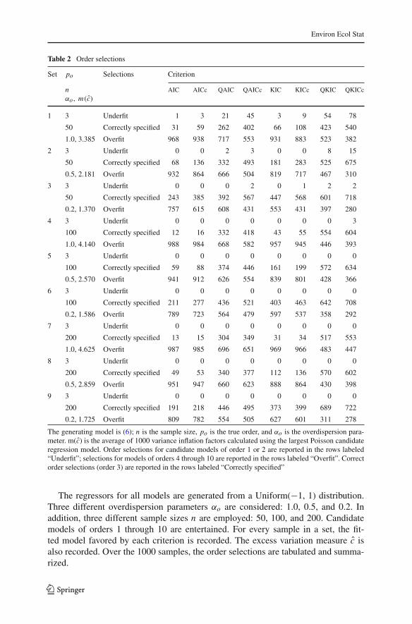
The regressors for all models are generated from a Uniform(−1, 1) distribution.Three different overdispersion parameters αo are considered: 1.0, 0.5, and 0.2. Inaddition, three different sample sizes n are employed: 50, 100, and 200. Candidatemodels of orders 1 through 10 are entertained. For every sample in a set, the fit-ted model favored by each criterion is recorded. The excess variation measure c isalso recorded. Over the 1000 samples, the order selections are tabulated and summa-rized.

123

Environ Ecol Stat




1 3 Underfit 70 107 121 193 151 207 239 318


1.0, 1.321 Overfit 489 312 353 171 268 167 154 86

2 3 Underfit 6 15 17 33 25 31 43 69


0.5, 1.323 Overfit 576 376 408 203 330 187 181 96

3 3 Underfit 1 1 1 2 2 2 3 5


0.2, 1.329 Overfit 475 284 307 127 239 127 120 54

4 3 Underfit 8 10 11 15 21 24 24 30


1.0, 1.011 Overfit 461 371 485 357 245 202 241 192

5 3 Underfit 0 0 0 0 0 0 0 0


0.5, 1.052 Overfit 506 435 489 380 307 235 279 203

6 3 Underfit 0 0 0 0 0 0 0 0


0.2, 1.109 Overfit 498 406 441 329 268 204 222 160

7 3 Underfit 0 0 0 0 0 0 0 0


1.0, 2.651 Overfit 287 248 29 24 115 102 6 5

8 3 Underfit 0 0 0 0 0 0 0 0


0.5, 2.129 Overfit 311 268 64 55 130 111 22 18

9 3 Underfit 0 0 0 0 0 0 0 0


0.2, 1.570 Overfit 308 265 137 105 141 121 47 38

The generating model is (6); n is the sample size, po is the true order, and αo is the overdispersionparameter. m(c) is the average of 1000 variance inflation factors calculated using the largest NEGBIN1candidate regression model. Order selections for candidate models of order 1 or 2 are reported in the rowslabeled “Underfit”; selections for models of orders 4 through 10 are reported in the rows labeled “Overfit”.Correct order selections (order 3) are reported in the rows labeled “Correctly specified”

The order selection results for the Poisson (3.2.1), NEGBIN1 (3.2.2), and NEGBIN2(3.2.3) candidate families are featured in Tables 2, 3, and 4, respectively. As with thesimulation results reported in Sect. 3.1, each quasi-likelihood criterion outperforms thecorresponding criterion based on the ordinary likelihood. This tendency is especiallyevident in those sets where the degree of excess dispersion is pronounced. In addi-tion, each J -divergence criterion obtains more correct selections than its I -divergencecounterpart, and each “corrected” criterion outperforms its non-adjusted counterpart.

123

Environ Ecol Stat




1 3 Underfit 38 60 55 91 82 120 116 160


1.0, 1.184 Overfit 375 216 283 123 164 91 110 47

2 3 Underfit 3 6 7 19 14 24 27 37


0.5, 1.244 Overfit 368 208 257 105 159 87 97 46

3 3 Underfit 1 1 1 3 2 2 5 7


0.2, 1.283 Overfit 392 238 271 136 208 104 121 59

4 3 Underfit 0 0 0 0 0 0 0 0


1.0, 1.095 Overfit 325 239 297 206 136 107 126 92

5 3 Underfit 0 0 0 0 0 0 0 0


0.5, 1.095 Overfit 336 251 281 209 149 114 121 97

6 3 Underfit 0 0 0 0 0 0 0 0


0.2, 1.119 Overfit 330 259 275 195 155 111 115 83

7 3 Underfit 0 0 0 0 0 0 0 0


1.0, 1.017 Overfit 294 265 287 250 130 107 122 105

8 3 Underfit 0 0 0 0 0 0 0 0


0.5, 1.037 Overfit 300 267 291 248 140 118 133 112

9 3 Underfit 0 0 0 0 0 0 0 0


0.2, 1.046 Overfit 285 239 263 216 106 91 101 82

The generating model is (6); n is the sample size, po is the true order, and αo is the overdispersionparameter. m(c) is the average of 1000 variance inflation factors calculated using the largest NEGBIN2candidate regression model. Order selections for candidate models of order 1 or 2 are reported in the rowslabeled “Underfit”; selections for models of orders 4 through 10 are reported in the rows labeled “Overfit”.Correct order selections (order 3) are reported in the rows labeled “Correctly specified”

In the NEGBIN2 framework, where the variance structure is correctly specified,the selection results in Table 4 are comparable to those in Table 1. However, in thePoisson and NEGBIN1 frameworks, the frequencies of correct order selections inTable 2 are smaller than those reported in Table 1. With the Poisson simulations, thecorrect selection rates for the likelihood-based criteria are often quite poor. Thesepatterns might be expected since the Poisson models ignore the overdispersion andthe NEGBIN1 models mischaracterize it. In particular, with severe overdispersion, it

123

Environ Ecol Stat

is clear that Poisson regression models are inadequate. Yet even in such settings, thequasi-likelihood criteria still choose the correct variable sets more often than the othercriteria. In general, over all of the sets, QKICc obtains the most correct selections,followed by QKIC and QAICc.

In the Poisson setting, a value of 1.0 for αo often leads to mean values for thevariance inflation factor c that exceed 4. From a practical perspective, such a largevalue for c indicates the need for a structural change in the model. In the NEGBIN1 andNEGBIN2 settings, the majority of the mean c values are very close to 1 and all are inthe 1–4 range. Such values imply that the degree of excess dispersion is not too severe,and that the variance structure is acceptable. Of course, in the NEGBIN2 framework,the variance structure of the candidate family is properly specified, meaning that thevalues of c should be quite close to 1. Although the mean values of c are near 1 for thesets based on larger sample sizes (n = 100, 200), the mean values are slightly largerthan 1 for the sets based on the smaller sample size (n = 50), reflecting a positive biasthat dissipates as the sample size increases.

With smaller sample sizes, we note that the glm, gamlss, and glm.nb functions in Rmay exhibit convergence problems for certain samples. The use of standard nonlinearoptimization algorithms for GLM maximum likelihood estimation is usually justified,yet issues may arise in simulation studies based on a large number of replications.A small percentage of generated samples led to fitted candidate models that did notconverge. Such samples were detected and omitted from the compilation of the results.We note that the selection patterns of the criteria do not seem to be affected by theinfrequent deletion of these samples.

4 Application

4.1 Introduction

The host-tick relationship is a complex interaction that can result in a differentialdistribution of ticks within a single host population. The factors contributing to varia-tion in tick burden among individuals within a population are likely cryptic. Attemptsto model these factors have elucidated some general trends, but have also failed tofind the specific attribute or suite of attributes that cause the heterogeneities seen inmany host-parasite systems (Brunner and Ostfeld 2008). Commonly examined hostattributes potentially important in predicting tick burdens are host sex (Zuk and McK-ean 1996; Klein 2000), body mass (Mooring et al. 2000), and age (Schalk and Forbes1997). Other abiotic factors such as seasonality (Krasnov et al. 2005) and meteorolog-ical variables (Harlan and Foster 1990) have also been shown to affect the host-tickrelationship, likely through differences in life history strategies or behavior at differenttimes of the year.

In Adair County, Missouri, the white-footed mouse (Peromyscus leucopus) andthe immature stages (larval and nymphal) of the American dog tick (Dermacentorvariabilis) form a host-specific relationship despite the presence of other potentialhost species (e.g. Microtus ochrogaster, Cryptotis parva, Tamias striatus, Reithrodon-tomys megalotis) (Kollars 1996). Within this host-parasite system, there is a large

123

Environ Ecol Stat

degree of heterogeneity in tick burdens on particular individuals. This may result inan increased probability of pathogen transmission (Woolhouse et al. 1997; Perkinset al. 2003). Additionally, differential parasitism can affect host population dynamicsthrough mortality and selective predation of infested individuals (Anderson and May1978). Despite some studies indicating that differential tick burdens did not negativelyinfluence host fitness (Brunner and Ostfeld 2008), other studies point to the energeticcost of blood regeneration and increased likelihood for pathogen transmission as fit-ness costs (Musante et al. 2007; Perkins et al. 2003).

Determining the cause of the heterogeneities in tick burdens could yield predictivedisease models and a better understanding of host-parasite interactions. The currentstudy aims to examine the factors that influence larval D. variabilis burdens on P.leucopus. The effect of habitat, number of nymphal D. variabilis present, host bodymass, host sex, tail length and right hind foot length will be examined using negativebinomial regression. Candidate models will be evaluated based on the selection criteriapreviously introduced.

4.2 Methods

4.2.1 Study site

The current study was conducted at long term monitoring sites in Adair County, Mis-souri in two different habitats. The habitats consisted of an early successional forestand an old field dominated by nonnative grasses. These sites were located approx-imately 300 meters apart and were therefore exposed to similar abiotic conditionsthroughout the study period.

4.2.2 Trapping

Trapping in each site was performed on a permanent trapping grid, containing 104sampling points. Each sampling point contained a Sherman live trap (H. B. Sherman,Tallahassee, Florida, USA) baited with a mixture of peanut butter and rolled oats.Trapping was performed concurrently on both grids every other month from June 2006to December 2008 for approximately 9,500 trap nights. Trapping sessions consisted of3-4 days of mark-recapture sampling with traps checked each morning. Each animalcaptured from both sites (X1, 1: forest, 2: field) was subjected to determination ofweight (X2, gram), sex (X3, 1: female, 2: male), right hind foot (X4, millimeter) andtail length (X5, millimeter), and removal of ticks. Ticks were stored in ethanol forlater identification of life stage (X6: the number of nymphal ticks). Animals weremarked with a toe-clip number for the purpose of identifying recapture in accordancewith the Animal Care and Use Committee standards of the American Society ofMammalogists (American Society of Mammalogists (1998)). From the total data, 172first capture P. leucopus individuals were used for this analysis. The data is availableat http://hjkim.sites.truman.edu/research.

Table 5 features basic descriptive statistics for the independent variables: specif-ically, proportions for habitat and gender, as well as means, variances, and pairwisecorrelation coefficients for the quantitative variables.

123

Environ Ecol Stat

Table 5 Descriptive statistics for independent variables

Site Forest (76.16 %) Field (23.84 %)

Sex Female (42.44 %) Male (57.56 %)

Mean Standard deviation Correlation coefficients

Weight Foot length Tail length Nymphal ticks

Weight 20.312 4.0911 0.2408 0.5845 −0.0959

Foot length 20.5232 1.1210 0.1877 0.0127

Tail length 73.5174 7.0433 0.0621

Nymphal ticks 0.5523 1.3476

4.2.3 Analysis

The analysis of the data proceeded by first selecting a suitable variance structure.Poisson, NEGBIN1, and NEGBIN2 regression models containing all 6 variables werefit to the data, and a distribution was chosen after an inspection of the values ofthe variance inflation factor c and AIC. With the chosen distribution, fitted candidatemodels based on all possible combinations of the 6 variables were compared relative toone another using values of AIC, AICc, QAIC, QAICc, KIC, KICc, QKIC, and QKICc.An optimal fitted model was determined based on the model selection criteria.

4.3 Model selection results

The average larval tick burden per P. leucopus individual was 3.24 and the variancewas 106.06. As the variance is substantially larger than the mean, overdispersion maybe present. The variance inflation factor c and AIC values were calculated for Poisson,NEGBIN1, and NEGBIN2 regression models with all 6 variables. The results are asfollows.

Fitted model Variance inflation factor (c) AIC

Poisson 20.55 1808.21

NEGBIN1 1.78 635.00

NEGBIN2 1.23 633.21

The variance inflation factor c, reflecting the excess dispersion that is not accommo-dated by the variance structure, was 20.55 when fitting the largest Poisson regressionmodel. When fitting the largest NEGBIN1 and NEGBIN2 regression models, thevalues of c were 1.78 and 1.23, respectively. These values of c suggest that excessdispersion exists under all three models, yet points to NEGBIN2 regression as themost suitable modeling framework. The NEGBIN2 model also has the smallest AICvalue, 633.21, lending additional support to the NEGBIN2 framework. The propriety

123

Environ Ecol Stat

Table 6 Best subsets among candidate models based on model selection criteria

Number ofvariables

Variable(s)included

Criterion

AIC AICc QAIC QAICc KIC KICc QKIC QKICc

1 x2 637.83 638.07 520.62 520.86 641.83 643.14 524.62 525.93

x3 639.61 639.85 522.07 522.31 643.61 644.93 526.07 527.39

2 x2, x6 634.68 635.04 518.43 518.79 639.68 641.15 523.43 524.90

x2, x3 637.31 637.67 520.57 520.93 642.31 643.78 525.57 527.04

3 x1, x2, x6 633.10 633.61 517.52 518.03 639.10 640.76 523.52 525.17

x2, x3, x6 635.54 636.05 519.50 520.01 641.54 643.20 525.50 527.16

4 x1, x2, x4, x6 633.01 633.69 517.81 518.50 640.01 641.88 524.81 526.69

x1, x2, x5, x6 633.40 634.08 518.13 518.81 640.40 642.27 525.13 527.00

5 x1, x2, x4,

x5, x6

634.10 634.98 519.07 519.96 642.10 644.23 527.07 529.20

x1, x2, x3,

x4, x6

634.20 635.08 519.16 520.04 642.20 644.33 527.07 529.20

6 x1, x2, x3,

x4, x5, x6

635.21 636.32 520.35 521.46 644.21 646.62 529.35 531.76

of NEGBIN2 models has been extensively supported by analyses that attempt to char-acterize factors influencing parasite infestations (Brunner and Ostfeld 2008; Shaw etal. 1998).

Among the NEGBIN2 candidate models summarized in Table 6, the model con-taining habitat, host body mass, tail length, and the number of nymphal ticks hadthe lowest AIC value. The model containing habitat, host body mass, and the num-ber of nymphal ticks had the lowest AICc, KIC, and KICc values. The modelcontaining host body mass and nymphal load had the lowest values of QKIC andQKICc.

It is not clear which model is “best” since the criteria choose different candidatemodels. However, based on the sample size (n = 172) and the value of the vari-ance inflation factor (c = 1.23), the simulation results provide some guidance. Insettings where the sample size is large and the degree of overdispersion is modest,AIC and AICc tend to choose over parameterized models. Also, the quasi-likelihoodcriteria outperform the ordinary likelihood criteria, and each J -divergence crite-rion outperforms its I -divergence counterpart. Based on these considerations, themodel chosen by QKIC and QKICc based on host body mass (x2i ) and nymphalload (x6i ) might be considered as the optimal candidate. This fitted model can bewritten as

ln(λi ) = −1.5229 + 0.1154x2i + 0.3027x6i , (7)

implying that there is positive relationship between larval D. variabilis burdens andthe body mass of P. leucopus and between larval and nymphal D. variabilis burdens.For this model, the MLE of overdispersion parameter, α, is 4.78.

123

Environ Ecol Stat

0 50 100 150

−20

020

4060

80

index

resi

dual

bas

ed o

n m

odel

(7)

Fig. 1 Residuals versus index based on the size of the predicted value (model (7))

To illustrate the predictive properties of model (7), Figure 1 features a plot ofthe residuals versus an index based on the size of the predicted value: i.e., index 1represents the smallest predicted value, index 2 represents the next largest predictedvalue, . . ., index n represents the largest predicted value. The figure illustrates a coupleof important properties regarding the predictive efficacy of the fitted model. First, mostof the residuals are small. In fact, 40% of the residuals are less than 2 in magnitude,65% of the residuals are less than 3 in magnitude, and 85% of the residuals are less than5 in magnitude. Second, the residuals tend to increase as the index for the predictedvalues increases, consistent with the notion of overdispersion. Thus, the model tendsto predict the response more accurately when the response is small.

4.4 Discussion

Our study found evidence that larval D. variabilis burdens were strongly associatedwith host body mass. The positive relationship between larval tick burdens and bodymass could be a function of increased surface area to mass ratio resulting in higherencounter probabilities as seen in South African ungulates (Gallivan and Horak 1997),differential energetic demands causing the hosts to forage more, and/or decreasedgrooming rates in larger individuals (Mooring et al. 2000).

Model selection criteria also suggested the positive relationship between larval andnymphal tick load. Nymphal ticks are larger and inflict a higher energetic cost to thehost relative to larvae, as they take a larger bloodmeal. The presence of nymphal tickscould cause the host to enter a negative feedback cycle, in which it needs to foragemore extensively to attempt to mount an immune response to the ticks present, butacquires more ticks through the extensive foraging.

123

Environ Ecol Stat

The lack of the significance of host sex in our study is a surprising finding, asanalyses based on data from the same location found a significant effect of sex inpredicting tick burdens (Dallas et al. 2012). However, these analyses were based onconventional model selection criteria such as AIC, AICc, KIC, and KICc using larvaland nymphal ticks combined. The final model based on the quasi-likelihood selectioncriteria QKIC and QKICc suggests that sex is not a major factor influencing the numberof larval ticks. While sex biased parasitism is a common trend (Zuk and McKean 1996;Klein 2000), it is not ubiquitous (Brunner and Ostfeld 2008; Wilson et al. 2002). Itis possible that larval ticks cannot discern between male and female hosts after hostacquisition, as Dukes and Rodriquez (1976) suggest based on data relating to hostodor. Additionally, larval ticks are opportunistic in their host selection, rarely movingmore than a few meters away from the site of oviposition (Sonenshine 1991).

The non-significant effect of tail and right hind foot length is not surprising, asthese measures are traditionally used to determine species and are not likely relatedto individual susceptibility to parasites.

5 Conclusion

Our results support three conclusions regarding model selection criteria based onKullback information measures. First, when dealing with overdispersed count data, thequasi-likelihood criteria tend to outperform the ordinary likelihood criteria. Second,for the purpose of delineating between correctly specified and misspecified models,the symmetric divergence may serve as a more sensitive discrepancy measure thanthe directed divergence. Third, the performance of a criterion appears to be dictatedby how well its penalty term corrects for the negative bias in the goodness-of-fitterm.

The ambiguity of an optimal model is illustrated by differences in the modelspreferred by various selection criteria. This phenomenon occurs both in our simulationstudies and in our application. Studies relying solely on a classical criterion such asAIC may therefore misinterpret the importance of the variables considered in candidatemodels.

In settings where overdispersion is suspected, formulating a family of candidatemodels based on a distribution that accommodates overdispersion may be a betteranalytical approach than formulating a family based on a conventional distribution(e.g., Poisson, binomial), and attempting to capture the excess variation via a simplevariance inflation factor. The former setting was considered in the first simulation study(Table 1); the latter setting was considered in the first part of the second study (Table2). The superiority of the selection results in the first study indicates that appropriatemean structures may be more easily identified when the analyst employs a distributiondesigned for overdispersed data. An extensive collection of simulation sets not featuredhere convey similar selection patterns.

Acknowledgments The authors wish to extend their appreciation to the anonymous reviewers for carefullyreading the previous versions of this manuscript, and for providing constructive suggestions that served toimprove the simulation study and the application.

123

Environ Ecol Stat

References

Agresti A (2002) Categorical data analysis, 2nd edn. Wiley, HobokenAkaike H (1973) Information theory and an extension of the maximum likelihood principle. In: Petrov BN,

Csáki F (eds) 2nd international symposium on information theory. Akadémia Kiadó, Budapest, Hungary,pp 267–281

Akaike H (1974) A new look at the statistical model identification. IEEE Trans Autom Control AC 19:716–723

American Society of Mammalogists (1998) Guidelines for the capture, handling, and care of mammals asapproved by the American Society of Mammalogists. J Mammal 79(4):1416–1431

Anderson DR, Burnham KP, White G (1994) Akaike information criterion model selection in overdispersedcapture-recapture data. Ecol Soc Am 75:1780–1793

Anderson RM, May RM (1978) Regulation and stability of host-parasite population interactions. J AnimalEcol 47:219–267

Brunner JL, Ostfeld RS (2008) Multiple causes of variable tick burdens on small-mammal hosts. Ecology89(8):2259–2272

Burnham KP, Anderson DR (2002) Model selection and multimodel inference. Springer, New YorkCavanaugh JE (1999) A large-sample model selection criterion based on Kullback’s symmetric divergence.

Stat Probab Lett 42:333–343Cavanaugh JE (2004) Criteria for linear model selection based on Kullback’s symmetric divergence. Aust

N Z J Stat 46:257–274Dallas T, Foré SA, Kim H-J (2012) Modeling the influence of Peromyscus leucopus body mass, sex, and

habitat on immature Dermacentor variabilis burden. J Vector Ecol 37(2):338–341Dukes JC, Rodriquez J (1976) A bioassay for host-seeking responses of tick nymphs (ixodidae). J Kansas

Entomol Soc 49(4):562–566Eberhardt LL (1978) Appraising variability in population studies. J Wildl Manag 42:207–238Gallivan G, Horak I (1997) Body size and habitat as determinants of tick infestations of wild ungulates in

south Africa. S Afr J Wildl Res 27(2):63–70Harlan H, Foster WA (1990) Micrometeorologic factors affecting field host-seeking activity of adult Der-

macentor variabilis (acari:ixodidae). J Med Entomol 27(4):471–479Hilbe JM (2008) Negative binomial regression. Cambridge University Press, UKHurvich CM, Tsai CL (1989) Regression and time series model selection in small samples. Biometrika

76:297–307Hurvich CM, Tsai CL (1995) Model selection for extended quasi-likelihood models in small samples.

Biometrika 51:1077–1084Hurvich CM, Shumway RH, Tsai CL (1990) Improved estimators of Kullback-Leibler information for

autoregressive model selection in small samples. Biometrika 77:297–307Johnson J, Omland K (2004) Model selection in ecology and evolution. TRENDS Ecol Evol 19(2):101–108Kim H-J, Cavanaugh JE (2005) Model selection criteria based on Kullback information measures for

nonlinear regression. J Stat Plan Inference 134(2):332–349Klein S (2000) The effects of hormones on sex differences in infection: from genes to behavior. Neurosci

Biobehav Rev 24(6):627–638Kollars T (1996) Interspecific differences between small mammals as hosts of immature Dermacentor

variabilis (Acari: Ixodidae) and a model for detection of high risk areas of rocky mountain spotted fever.J Parasitol 82(5):707–710

Krasnov BR, Morand S, Hawlena H, Khokhlova IS, Shenbrot GI (2005) Sex-biased parasitism, seasonality,and sexual size dimorphism in desert rodents. Oecologia 146(2):209–217

Kullback S (1968) Information theory and statistics. Dover, MineolaLebreton J, Burnham K, Clobert J, Anderson D (1992) Model survival and testing biological hypotheses

using marked animals: a unified approach with case studies. Ecol Monogr 62(1):67–118Meinshausen N (2007) Relaxed Lasso. Comput Stat Data Anal 52:374–393Min A, Holzmann H, Czado C (2010) Model selection strategies for identifying most relevant covariates

in homoscedastic linear model. Comput Stat Data Anal 54(12):3194–3211Mooring M, Benjamin J, Harte C, Herzog N (2000) Testing the interspecific body size principle in ungulates:

the smaller they come, the harder they groom. Animal Behav 60(1):35–45Musante AR, Pekins PJ, Scarpitti DL (2007) Metabolic impacts of winter tick infestations on calf moose.

Alces 43:101–107

123

Environ Ecol Stat

Perkins SE, Cattadori IM, Tagliapietra V, Rizzoli AP, Hudson PJ (2003) Empirical evidence for key hostsin persistence of a tick-borne disease. Int J Parasitol 33:909–917

R Development Core Team (2009) R: a language and environment for statistical computing. R foundationfor statistical computing, Vienna, Austria

Schalk G, Forbes MR (1997) Male biases in parasitism of mammals: effects of study type, host age, andparasite taxon. Oikos 78:67–79

Shaw D, Grenfell B, Dobson A (1998) Patterns of macroparasite aggregation in wildlife host populations.Parasitology 117:597–610

Sonenshine D (1991) The biology of ticks. Oxford University Press, New YorkSugiura N (1978) Further analysis of the data by Akaike’s information criterion and the finite corrections.

Commun Stat A7:13–26Tibshirani R (1996) Regression shrinkage and selection via the Lasso. J R Stat Soc B 58:267–288Wang H, Leng C (2008) A note on adaptive group Lasso. Comput Stat Data Anal 52:5277–5286Wedderburn RWM (1974) Quasilikelihood functions, generalized linear models and the Gauss-Newton

method. Biometrika 61:43–47Wilson K, Bjornstad O, Dobson A, Merler S, Poglayen G, Randolph S, Read A, Skorping A (2002) Het-

erogeneities in macroparasite infections: patterns and processes. In: Hudson PJ, Rizzoli A, Grenfell BT,Heesterbeek H, Dobson AP (eds) The ecology of wildlife diseases. Oxford University Press, New York

Woolhouse M, Dye C, Etard J, Smith T, Charlwood J, Garnett G, Hagan P, Hii J, Ndhlovu P, Quinnell R,Watts C, Chandiwana S, Anderson R (1997) Heterogeneities in the transmission of infectious agents:implications for the design of control programs. Natl Acad Sci USA 94:338–342

Zuk M, McKean KA (1996) Sex differences in parasite infections: patterns and processes. Int J Parasitol26(10):1009–1024

Author Biographies

Hyun-Joo Kim received a Ph.D. degree in Statistics from the University of Missouri-Columbia in 2000.In 2000, she joined the Department of Mathematics and Computer Science at Truman State Univer-sity, Missouri. She is currently a full professor of Statistics at the Department of Statistics. In 2010, shefounded the Center for Applied Statistics and Evaluation and has been the director of the center. Her cur-rent research interests include environmental statistics, model selection, and statistical consulting.

Joseph E. Cavanaugh received B.S. degrees in Computer Science and Mathematics from Montana Techin 1986, an M.S. degree in Statistics from Montana State University in 1988, and a Ph.D. degree in Sta-tistics from the University of California, Davis, in 1993. From 1993 to 2003, he was on the faculty of theDepartment of Statistics at the University of Missouri—Columbia. He is currently Professor and Directorof Graduate Studies in the Department of Biostatistics at the University of Iowa. He holds a secondaryappointment in the Department of Statistics and Actuarial Science. His methodological research interestsinclude model selection and time series analysis.

Tad A. Dallas graduated from Truman State University, Missouri, in 2010 with his M.Sc. in biology. In2011, he worked in a United States Department of Agriculture laboratory in Fort Pierce, Florida, exam-ining pathogens of citrus crops. Since 2011, he has been working towards his Ph.D. at the University inGeorgia’s Odum School of Ecology in the lab of Dr. John Drake, where his research interests focus onhost-pathogen interactions in a population and community context.

Stephanie A. Foré graduated from Miami University, Ohio, USA with a Ph.D. in Botany in 1991. Sheis currently a full professor of biology at Truman State University, Missouri, USA. Her current researchis focused on the ecology of ticks.

123

Documents

Model selection criteria for overdispersed data and their application to the characterization of a host-parasite relationship