Model Regresi Untuk Data Deret Waktu (1)Pika Silvianti, M.Sipikasilvianti@apps.ipb.ac.idSumber: Hyndman, R.J and Athanasopoulos, G. 2013. Forecasting: principles and practicehttps://www.otexts.org/fpp/4

Review model regresi

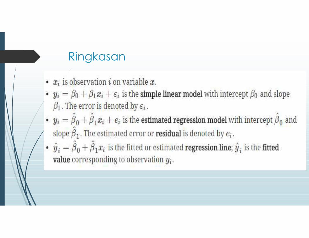
forecast variable y is sometimes also called the regressand, dependent or explained variable.

predictor variable x is sometimes also called the regressor, independent or explanatory variable.

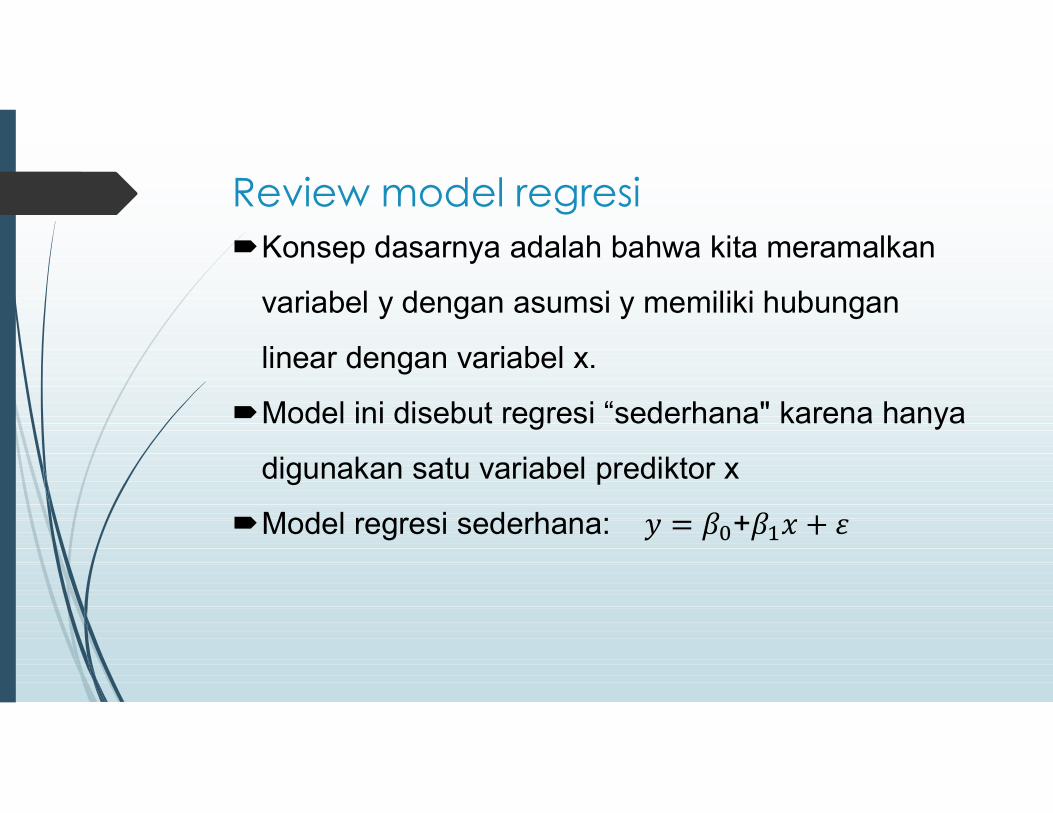
Review model regresiKonsep dasarnya adalah bahwa kita meramalkan

variabel y dengan asumsi y memiliki hubunganlinear dengan variabel x.

Model ini disebut regresi “sederhana" karena hanyadigunakan satu variabel prediktor x

Model regresi sederhana: +

Ringkasan

Asumsi untuk error Nilai tengahnya 0; jika tidak, hasil ramalannya akan mengalami bias

sistematikContoh bias sistematis termometer yang selalu membaca tiga derajat lebihdingin dari suhu yang sebenarnya karena kalibrasi awal yang salah

Tidak berkorelasi diri (autocorrelated); jika berkorelasi diri, makaramalannya tidak efisien karena ada informasi lebih lanjut untukdieksploitasi dalam data.

tidak terkait dengan variabel prediktor; kalau tidak ,akan adainformasi lebih lanjut yang harus dimasukkan di bagian sistematisdari model.

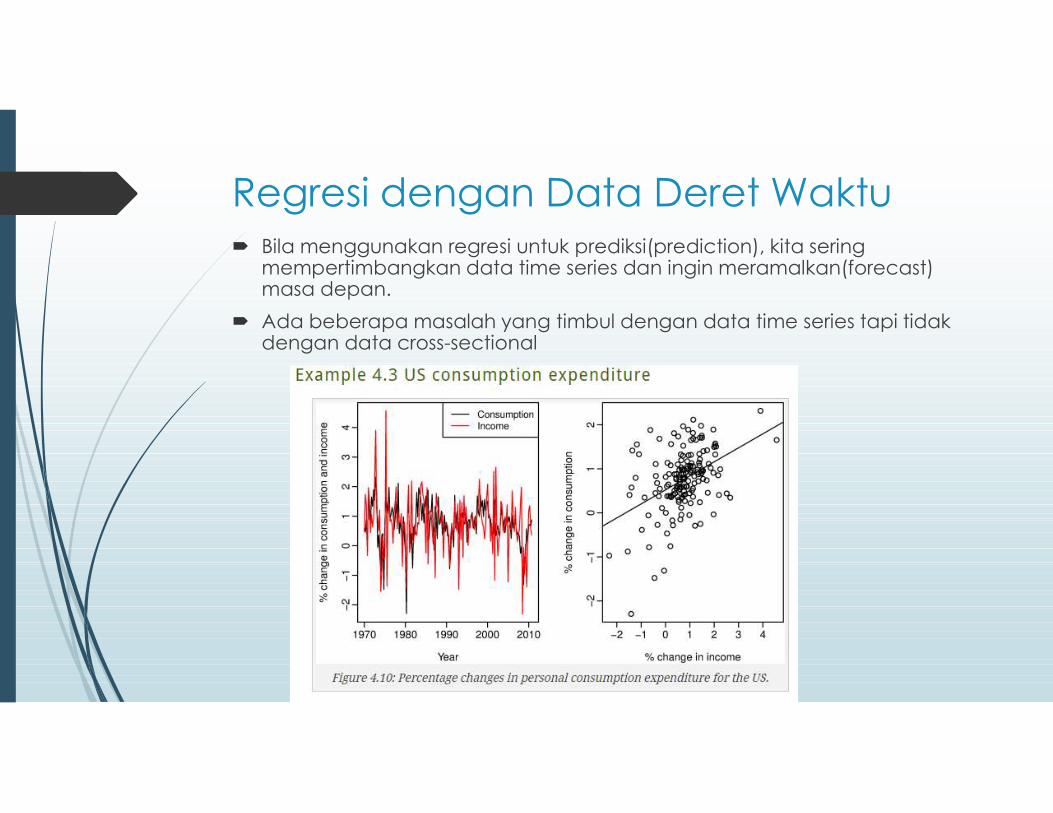
Regresi dengan Data Deret Waktu Bila menggunakan regresi untuk prediksi(prediction), kita seringmempertimbangkan data time series dan ingin meramalkan(forecast) masa depan. Ada beberapa masalah yang timbul dengan data time series tapi tidakdengan data cross-sectional

Figure 4.10 shows time series plots of quarterly percentage changes (growth rates) of real personal consumption expenditure (CC) and real personal disposable income (II) for the US for the period March 1970 to Dec 2010.

these show that a 1% increase in personal disposable

income will result to an average increase of 0.84% in personal consumption expenditure.

We are interested in forecasting consumption for the four quarters of 2011.

variabel prediktor (income dalam hal ini) diperlukanuntuk dimasukkan ke dalam model regresi , tetapinilai ini tidak diketahui sebelumnya.

Salah satu solusi untuk masalah ini adalah denganmenggunakan " scenario based forecasting ".

Scenario based forecasting

peramal berasumsi skenario yang mungkin untuk variabel predictor. Misalnya pembuat kebijakan AS mungkin ingin meramalkankonsumsi jika ada pertumbuhan 1%income untuk setiap kuartalpada tahun 2011. Atau penurunan 1% income untuk masing-masingkuartal.

Peramalan yang dihasilkan dihitung dan ditunjukkan pada Gambar4.11.

Selang peramalan untuk for scenario based forecasts tidaktermasuk ketidakpastian terkait dengan nilai-nilai masa depanvariabel prediktor. Mereka menganggap nilai prediktor yang diketahui sebelumnya.

Pendekatan alternatif adalah dengan menggunakan peramalanasli untuk variabel prediktor. Misalnya, pendekatan time series murnidapat digunakan untuk menghasilkan peramalan untuk variabelprediktor atau perkiraan yang diterbitkan oleh beberapa sumberlain seperti lembaga pemerintah dapat digunakan.

Ex-ante versus ex-post forecasts Ex ante forecasts are those that are made using only the

information that is available in advance. For example, ex ante forecasts of consumption for the four quarters in 2011 should only use

information that was available before 2011. These are the only genuine forecasts, made in advance using whatever information is available at the time.

Ex post forecasts are those that are made using later information on the predictors. For example, ex post forecasts of consumption for each of the 2011 quarters may use the

actual observations of income for each of these quarters, once these have been observed. These are not genuine forecasts, but are useful for studying the behaviour of forecasting models.

Example 4.4 Linear trend

Residual autocorrelation Regresi data deret waktu residual pasti memiliki korelasi diri Dugaan model melanggar asumsi tidak ada autokorelasi dalam residual, peramalan mungkin tidak efisien - ada beberapa informasi yang tersisa

yang harus dimanfaatkan untuk mendapatkan peramalan yang lebih baik. Peramalan dari model dengan residual yg berkorelasi diri masih tidak bias,

dan juga tidak "salah", tetapi biasanya akan memiliki selang prediksi yang lebih besar.

ExerciseDay 1 2 3 4 5 6 7 8 9 10 11 12Mwh 16.3 16.8 15.5 18.2 15.2 17.5 19.8 19.0 17.5 16.0 19.6 18.0temp 29.3 21.7 23.7 10.4 29.7 11.9 9.0 23.4 17.8 30.0 8.6 11.8

Electricity consumption was recorded for a small town on 12 randomly chosen days. The following maximum temperatures (degrees Celsius) and consumption (megawatt-hours) were recorded for each day.

a) Plot the data and find the regression model for Mwh with temperature as an explanatory variable. Why is there a negative relationship?

b) Produce a residual plot. Is the model adequate? Are there any outliers or influential observations?

c) Use the model to predict the electricity consumption that you would expect for a day with maximum temperature 10∘10∘ and a day with maximum temperature 35∘35∘. Do you believe these predictions?

d) Give prediction intervals for your forecasts. The following R code will get you started:

R COdeplot(Mwh ~ temp, data=econsumption)fit <- lm(Mwh ~ temp, data=econsumption)plot(residuals(fit) ~ temp, data=econsumption)forecast(fit, newdata=data.frame(temp=c(10,35)))