Embed Size (px)
Citation preview

CR2GConstraint Research and Reading Group
MODEL ORDER REDUCTIONUsing Cubic Spline Curve-Fitting
Leobardo Valera, Martine CeberioMiguel ArgaezDepartment of Computer ScienceComputational Science ProgramThe University of Texas at El Paso
Introduction Discretization. . . . . . .Reduction C-Splines Future Work
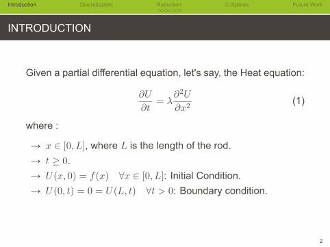
INTRODUCTION
Given a partial differential equation, let's say, the Heat equation:
∂U
∂t= λ
∂2U
∂x2(1)
where :
→ x ∈ [0, L], where L is the length of the rod.→ t ≥ 0.→ U(x, 0) = f(x) ∀x ∈ [0, L]: Initial Condition.→ U(0, t) = 0 = U(L, t) ∀t > 0: Boundary condition.
2

Introduction Discretization. . . . . . .Reduction C-Splines Future Work
DISCRETIZATION
If we discretize [0, L] taking ∆x = 10−2, in order to ensurequadratic convergence, we have to take ∆t ≤ 0.5× 10⁻⁴. Nowif 0 ≤ t ≤ 5, we have 100, 000 nodes in the temporal axis. Itmeans that we have to solve a linear system like:
Au = b (2)
100, 000 times.
As an example: If it takes 1 second to solve every linearsystem, it will take more than 27 hours to solve the wholeproblem.
It is imperative to Reduce the dimension of the problem.
3

Introduction Discretization. . . . . . .Reduction C-Splines Future Work
REDUCTION
In our example, the solution of our system is u ∈ R100. Let'sassume that we know, for some reason, that u ∈ S, where S isa 10−dimentional subspace of R100 with base W , then:
Wy = u (3)
Now, sustituting (3) in (2), we obtain:
(AW )y = b (4)
4
Introduction Discretization. . . . . . .Reduction C-Splines Future Work
REDUCTION
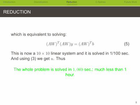
which is equivalent to solving:
(AW )T (AW )y = (AW )T b (5)
This is now a 10× 10 linear system and it is solved in 1/100 sec.And using (3) we get u. Thus
The whole problem is solved in 1, 000 sec.: much less than 1hour.
5

Introduction Discretization. . . . . . .Reduction C-Splines Future Work
HOW TO FIND A BASE W
Proper Orthogonal Decomposition
The idea with this method is that the time response of a system,given a certain input, contain the behavior of the system.
We have the following algorithm to obtain W .
1. Solve the full-order model for several values of λ.2. For each λ, take one or more snapshots, which is the
solution of (2) in some values of t, and store suchsnapshots in a matrix called X, for example.
6

Introduction Discretization. . . . . . .Reduction C-Splines Future Work
PROPER ORTHOGONAL DECOMPOSITION
7
Introduction Discretization. . . . . . .Reduction C-Splines Future Work
... HOW TO FIND A BASE W ...
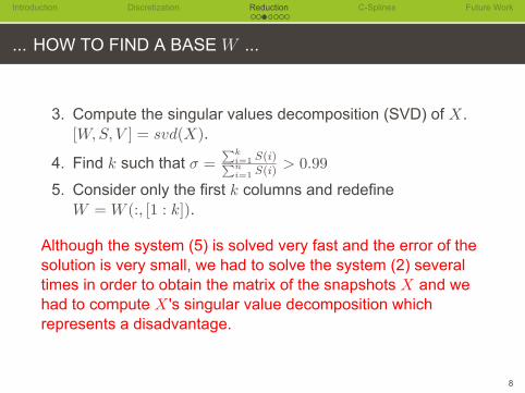
3. Compute the singular values decomposition (SVD) of X.[W,S, V ] = svd(X).
4. Find k such that σ =∑k
i=1 S(i)∑ni=1 S(i)
> 0.99
5. Consider only the first k columns and redefineW = W (:, [1 : k]).
Although the system (5) is solved very fast and the error of thesolution is very small, we had to solve the system (2) severaltimes in order to obtain the matrix of the snapshots X and wehad to compute X 's singular value decomposition whichrepresents a disadvantage.
8

Introduction Discretization. . . . . . .Reduction C-Splines Future Work
... HOW TO FIND A BASE W . WAVELETS
Let's assume the matrix A is the following image:
100 200 300 400 500 600
100
200
300
400
500
600
and
Φ =
(W T
HT
)where W T is the lowpass HT is the high pass
9

Introduction Discretization. . . . . . .Reduction C-Splines Future Work
... HOW TO FIND A BASE W ...
The product matrix AΦT will be;
100 200 300 400 500 600
100
200
300
400
500
600
AW AH
We save time computing W but when we use (3) to get theapproximation u, the error is greater than what the error weobtained using Proper Orthogonal Decomposition Method fromthe snapshots approach.
10

Introduction Discretization. . . . . . .Reduction C-Splines Future Work
IS THERE ANYTHING ELSE WE CAN DO?
So far we have:
Good
Bad
Good
Bad
Time Error
→ POD is "bad" in time and "good" in error→ Wavelets is "good" in time but "bad" in error
11

Introduction Discretization. . . . . . .Reduction C-Splines Future Work
YES, THERE IS SOMETHING ELSE WE CAN DO
We propose a "Midpoint"
Good
Bad
Good
Bad
Time Error
We propose a method in which we do not have to compute anybase and we get an acceptable error within a good computationtime. 12

Introduction Discretization. . . . . . .Reduction C-Splines Future Work
METHOD USING C-SPLINES
Our method is inspired by super-resolution methods and isbased on Spline Interpolation. x = 0:10; y = sin(x); xx =0:.25:10; yy = spline(x,y,xx); plot(x,y,'o',xx,yy)
0 1 2 3 4 5 6 7 8 9 10−1
−0.8
−0.6
−0.4
−0.2
0
0.2
0.4
0.6
0.8
1
13
Introduction Discretization. . . . . . .Reduction C-Splines Future Work
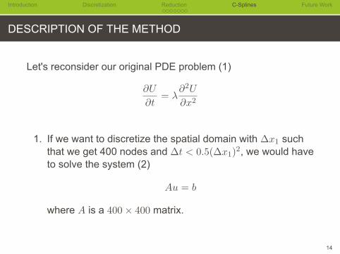
DESCRIPTION OF THE METHOD
Let's reconsider our original PDE problem (1)
∂U
∂t= λ
∂2U
∂x2
1. If we want to discretize the spatial domain with ∆x1 suchthat we get 400 nodes and ∆t < 0.5(∆x1)
2, we would haveto solve the system (2)
Au = b
where A is a 400× 400 matrix.
14

Introduction Discretization. . . . . . .Reduction C-Splines Future Work
...DESCRIPTION OF THE METHOD
2. Instead of discretizing the spatial domain with ∆x1, we canuse ∆x2 = 4∆x1, for instance, and then we obtain 100nodes and we keep the same ∆t. We solve the system (2)
Au = b
where A is a 100× 100 matrix.3. After we obtain u, we interpolate it using spline in order to
get an approximation of u.
15

Introduction Discretization. . . . . . .Reduction C-Splines Future Work
... DESCRIPTION. GRAPHIC VERSION
For each t, we have:
What we want
What we compute
What we getafter interpolating
x1 x2 x3 x4 x5 x6 x7 x8 x9 xn
u1 u2 u3 u4 u5 u6 u7 u8 u9 un· · ·
u1 u5 u9 u400· · ·
u1 u5 u9 u400· · ·u2 u3 u4 u6 u7 u8
· · ·
16

Introduction Discretization. . . . . . .Reduction C-Splines Future Work
EXAMPLE AND NUMERICAL RESULTS
Suppose we want solve
∂U
∂t= λ
∂2U
∂x2
with x ∈ [0, 1], ∆x = 0.0025, t ∈ [0, 0.01] with ∆t = 2.50× 10⁻⁶
and λ = 1.
Full- Order Model (FOM): Time to solve the problem and getUfom: t = 10.16 sec.
17
Introduction Discretization. . . . . . .Reduction C-Splines Future Work
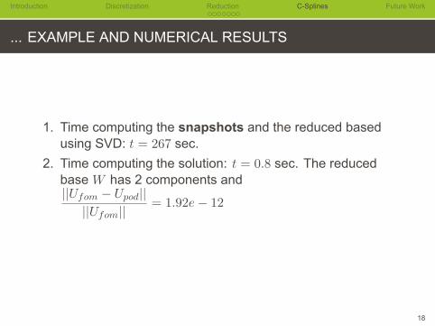
... EXAMPLE AND NUMERICAL RESULTS
1. Time computing the snapshots and the reduced basedusing SVD: t = 267 sec.
2. Time computing the solution: t = 0.8 sec. The reducedbase W has 2 components and||Ufom − Upod||
||Ufom||= 1.92e− 12
18

Introduction Discretization. . . . . . .Reduction C-Splines Future Work
FOM VS. POD
0 50 100 150 200 250 300 350 400 450−0.5
0
0.5
1
1.5
2Solution Computed with FOM and POD
Solution FOMSolution POD
19

Introduction Discretization. . . . . . .Reduction C-Splines Future Work
... EXAMPLE AND NUMERICAL RESULTS
1. Time computing the Wavelet Matrix Daubechies 2 withlevel 2: t = 0.047 sec.
2. Time computing the solution: t = 6.77 sec. The reduced
base W has 50 components and||Ufom − Uwav||
||Ufom||= 0.0046
20

Introduction Discretization. . . . . . .Reduction C-Splines Future Work
FOM VS. WAVELETS
0 50 100 150 200 250 300 350 400 450−0.5
0
0.5
1
1.5
2
x
u
Solution Computed with FOM and Wavelets
Solution FOM
Solution Wavelets
65 70 75 80 85 90 95 100 105 110 1151.35
1.4
1.45
1.5
1.55
1.6
1.65
x
u
Solution Computed with FOM and Wavelets
Solution FOM
Solution Wavelets
21

Introduction Discretization. . . . . . .Reduction C-Splines Future Work
... EXAMPLE AND NUMERICAL RESULTS
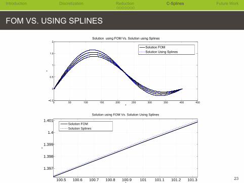
1. Time computing the solution using a coarse refinement:t = 0.69 sec.
2. Time interpolating using spline: t = 0.21 sec. and||Ufom − UCVM ||
||Ufom||= 4.09e− 05
22
Introduction Discretization. . . . . . .Reduction C-Splines Future Work
FOM VS. USING SPLINES
0 50 100 150 200 250 300 350 400 4500.5
0
0.5
1
1.5
2
x
u
Solution using FOM Vs. Solution using Splines
Solution FOM
Solution Using Splines
100.5 100.6 100.7 100.8 100.9 101 101.1 101.2 101.3
1.397
1.398
1.399
1.4
1.401
x
u
Solution using FOM Vs. Solution Using Splines
Solution FOMSolution Splines
23

Introduction Discretization. . . . . . .Reduction C-Splines Future Work
WAVELETS VS. USING SPLINES
65 70 75 80 85 90 95 100 105 110 1151.35
1.4
1.45
1.5
1.55
1.6
1.65
x
u
Solution Computed with FOM and Wavelets
Solution FOM
Solution Wavelets
100.5 100.6 100.7 100.8 100.9 101 101.1 101.2 101.3
1.397
1.398
1.399
1.4
1.401
x
u
Solution using FOM Vs. Solution Using Splines
Solution FOMSolution Splines
24

Introduction Discretization. . . . . . .Reduction C-Splines Future Work
SUMMARY
Method offline time online time ErrorFOM 10.16 secPOD 267 sec 0.8 sec 1.92e− 12
WAV 0.04 sec 6.77 sec 0.015
CVM 0.21 sec 0.69 sec 4.09e− 5
Good
Bad
Good
Bad
Time E
rror
25

Introduction Discretization. . . . . . .Reduction C-Splines Future Work
FUTURE WORK
1. We plan to use adaptive discretization to avoid losingprecision in case the solution has drastic changes ofbehavior.
2. We also plan to address the problem of non-linear PDEsusing similar approaches; for example, for the Burgersequations.
26

Introduction Discretization. . . . . . .Reduction C-Splines Future Work
REFERENCES
→ Wilhelmus H.A. Schilders, Henk A. van der Vorst, andJoost Rommes. 2008. Model Order Reduction. Theory,Research Aspects and Applications. Springer, BerlinHeidelberg.
→ Miguel Hernandez IV. 2013. Reduced-Order ModelingUsing Orthogonal and Bi-Orthogonal WaveletTransforms. Ph.D. Dissertation. Computational ScienceProgram, The University of Texas at El Paso.
→ Jean-Luc Starck, Fionn Murtagh, and Jalal M. Fadili. 2010.Sparse Image and Signal Processing. Wavelets,Curvelets, Morphological Diversity. Cambridg UniversityPress, 32 Avenue of the Americas, New York, NY.
27
Introduction Discretization. . . . . . .Reduction C-Splines Future Work
ACKNOWLEDGMENT
1. Dr. Martine Ceberio.
2. Dr. Miguel Argaez.3. The Graduate Student Research Expo's Organizators.4. Computational Sciences Program.5. La universidad Metropolitana. Caracas, Venezuela
28

Introduction Discretization. . . . . . .Reduction C-Splines Future Work
ACKNOWLEDGMENT
1. Dr. Martine Ceberio.2. Dr. Miguel Argaez.
3. The Graduate Student Research Expo's Organizators.4. Computational Sciences Program.5. La universidad Metropolitana. Caracas, Venezuela
28

Introduction Discretization. . . . . . .Reduction C-Splines Future Work
ACKNOWLEDGMENT
1. Dr. Martine Ceberio.2. Dr. Miguel Argaez.3. The Graduate Student Research Expo's Organizators.
4. Computational Sciences Program.5. La universidad Metropolitana. Caracas, Venezuela
28

Introduction Discretization. . . . . . .Reduction C-Splines Future Work
ACKNOWLEDGMENT
1. Dr. Martine Ceberio.2. Dr. Miguel Argaez.3. The Graduate Student Research Expo's Organizators.4. Computational Sciences Program.
5. La universidad Metropolitana. Caracas, Venezuela
28

Introduction Discretization. . . . . . .Reduction C-Splines Future Work
ACKNOWLEDGMENT
1. Dr. Martine Ceberio.2. Dr. Miguel Argaez.3. The Graduate Student Research Expo's Organizators.4. Computational Sciences Program.5. La universidad Metropolitana. Caracas, Venezuela
28

Introduction Discretization. . . . . . .Reduction C-Splines Future Work
THANKS!
Thanks!
29