1

Model identification of bridges using measurement data

Y. Robert-Nicoud, B. Raphael, O. Burdet and I.F.C. Smith

EPFL-Swiss Federal Institute of Technology

Structural Engineering Institute

CH-1015 Lausanne

Switzerland

ABSTRACT

Measurements are increasingly used to augment traditional assessments of structural

state. Measurements of deflections, rotations and strain provide indications of

damages as well as changes in the values of parameters such as Young’s modulus.

Finite element model updating methods have been developed in the 1990s for

identifying structural state from measurements. Currently most methods aim to

determine the values of stiffness coefficients that result in measured responses. In the

present work, a model calibration method identifies causes of structural behaviour

such as support conditions and material properties. Static measurement data is

employed for model calibration. A case study of the Lutrive bridge in Switzerland

illustrates the methodology. Candidate models whose responses reasonably match

measured data are identified. These models are then examined in order to determine

whether the calibrated values are physically possible. Such examinations lead to

either model rejection or further measurements.

1 Introduction

Traditionally structures are inspected by experts in order to determine whether they

are capable of satisfying strength and serviceability criteria. An increasing number of

structures are being equipped with measurement systems in order to augment

traditional assessments and to increase understanding of structural behavior. Although

measurements of deflections, rotations and strain provide indications of damages as

well as gradual deterioration in the structural state, interpretation of measurements for

obtaining metrics that directly indicate structural health or damage is not a well-

established science (Housner et al., 1997).

When a structure is monitored periodically, changes in deflection patterns are

potentially useful for determining whether material properties change with respect to

time and also to examine whether there is any damage after critical events. This

process is costly since measurements need to be taken several times a year. Another

complication is that deflection patterns are influenced by factors such as temperature

changes. However, if appropriate corrections to such effects are applied, data from

continuous monitoring, along with appropriate modeling, help determine gradual and

sudden changes in the structural state.

This is the peer reviewed version of the following article: Robert-Nicoud, Y., Raphael, B., Burdet, O. and Smith, I.F.C. "Model Identification of Bridges Using Measurement Data", Computer-Aided Civil and Infrastructure Engineering, Vol 20, no 2, 2005, pp 118-131 which has been published in final form at onlinelibrary.wiley.com/doi/10.1111/j.1467-8667.2005.00381This article may be used for non-commercial purposes in accordance with Wiley Terms and Conditions for Self-Archiving.

2

When it is not possible to take measurements several times a year, modeling

techniques remain useful for determining the structural state using a limited number

of tests. Such modeling may employ system identification methods. These methods

aim to compute the values of system parameters through a comparison of predicted

and observed responses. When the form of the relationship between observable

quantities and system parameters are known, regression techniques can be applied for

identifying system parameters. The strategy is to minimize the error between the

predicted output and measured values. This approach is common in dynamic systems

that are employed in electrical and mechanical engineering. Standard techniques exist

for selecting the model structure (form of the equation) from a set of candidate models

(Ljung 1999). However, these techniques are not applicable to structural engineering

systems because responses are highly non-linear with respect to model parameters.

Structures are usually analyzed by the finite element method for a known set of values

of parameters such as material properties, geometric properties and loading in order to

compute deflections and other responses such as mode shapes and frequencies.

However, there is rarely a reverse procedure that directly computes the material and

geometric properties from responses such as deflections. Procedures that aim to

estimate these quantities through minimizing the error between measured and

computed responses are known as finite element model updating techniques.

Currently, the most common method of damage detection using measurements is

through the use of vibration data. This is an active research area. Friswell and

Mottershead (1995) provide a survey of model updating procedures using vibration

measurements. Recent papers published in this area include, Brownjohn et al. (2003),

Castello et al. (2002), Teughels et al. (2002), Modak et al. (2002), Hemez and

Doebling (2001), Sohn and Law (2001), Hu et al. (2001), Reich and Park (2001),

Chaudhary et al. (2000), Yu et al. (1999), Abe (1998), Beck and Katafygiotis (1998),

Katafygiotis and Beck (1998), Park and Felippa, (1998), and Sohn and Law (1997).

Most work in this area aim to compute the set of stiffness coefficients that produce

observed vibration modes of structures. Location and extent of damage are inferred

through a comparison between the stiffness coefficients of the damaged and

undamaged structures.

Since model-updating procedures are generally developed for specific types of

responses, these procedures are not applicable to other response types. For example,

problem formulations have been developed for computing the set of stiffness

coefficients that produce observed vibration modes of structures. These formulations

cannot be used to determine unknown forces when there is uncertainty with respect to

the loading and environmental factors. Also, most methodologies are not able to

determine causes of abnormal structural behavior, such as settlement of supports and

cracking of concrete sections.

There are isolated reports of work involving static measurements to interpret

structural state. Model updating procedures using static measurements either use

deflection data or strain data. Papers that discuss model updating using deflection

data include, Hajela and Soeiro (1990), Sanayei and Onipede (1991), Sanayei and

Scamoli (1991), Banan and Hjelmstad (1994 a,b), Hjelmstad and Shin (1997).

Sanayei and Saletnik (1996) and Liu and Chian (1997) are examples of work

involving model updating using strain measurements. All of this work involves

3

formulation of appropriate optimization problems for the minimization of the error

between analytical and measured quantities for a given finite element model. The

number of unknown variables is fixed in each optimization problem. Models that

have varying number of degrees of freedom and consequently, different sets of

variables are not accommodated in such approaches.

In structural engineering, models cannot always be approximated by closed form

mathematical expressions and therefore, it is not possible to apply mathematical

methods for minimization of errors, such as those described in textbooks, for example

(Ljung 1999). Mathematical methods are not applicable when classes of models

containing different degrees of freedom (and consequently different forms of

equations) need to be searched to locate the minimum. In such situations, it is

necessary to utilize optimization methods that employ a “generate-test” methodology

(Raphael and Smith, 2003a). Optimization methods that make use of only the values

of the objective function and do not require additional information such as gradients

are generally known as direct search methods (Lewis et al. 2000). Points are

generated and tested for the satisfaction of objectives and constraints through the

evaluation of the objective function. The most widely used direct search techniques

are simulated annealing (Kirkpatrick et al. 1983, Martin, 1995), and genetic

algorithms (Holland 1975, Goldberg, 1989). Koh et al., (2003) use a combination of

genetic algorithms and local search techniques for the identification of structural

parameters using vibration measurements. Sharman and Esparcia-Alcazar (1993) use

a combination of genetic algorithm and simulated annealing to optimize both the

model structure and the numerical parameters of the model. Search techniques have

also been combined with qualitative reasoning for system identification. Recent

examples are found in Bradley et al. (2001) and Kay et al. (2000). Dunn (1998) uses a

combination of genetic algorithm and stochastic hill climbing to compute the stiffness

coefficients of a mass-spring system. Cunha et al. (1999) use genetic algorithm to

estimate the stiffness coefficients by minimizing a residual formed from the Eigen

solutions. Another example of the use of genetic algorithm for the determination of

stiffness reduction is Mares and Surace (1996). The main drawback of the above

methodologies is that causes of structural behavior cannot be easily determined using

the values of stiffness coefficients.

This paper describes an approach to making use of measurement data for performing

diagnostic assessments of structures. The overall project goal is to identify possible

causes of observed behaviour. Since it is not often possible to make definite

conclusions related to causes, the focus of the current study involves identifying

candidate models of behaviour. Model predictions that match measured values as

closely as possible are identified. An examination of the characteristics of these

models leads to explanations of observed behaviour. The outline of this paper is as

follows: measurement systems that have been used in the present study are discussed

in Section 2; the approach based on model identification and calibration is discussed

in Section 3; results are summarized in Section 4.

2 Measurement systems

Measurements that are useful for making diagnostic assessments of structures are

examined in this section. Three types of measurement systems have been used in the

present study. They are:

4

• Hydrostatic leveling

• Inclinometers

• Fiber optic sensors

Appropriate interpretations of the data that is collected by these systems are necessary

for structural evaluations. When applicable, such interpretations are discussed with

the descriptions given below.

2.1 Hydrostatic leveling

The hydrostatic leveling system (Burdet 1993, Favre et al. 1995) is based on the

principle of communicating vessels. The deflection at any point in the structure is

obtained by computing the sums and differences of measured levels at various points.

This system has the following advantages:

• It is easy to install and is inexpensive

• Discontinuous operations are possible, permitting the reactivation of an

unused system after years of discontinued service, provided that new tubing is

installed.

• Operation is possible even under heavy traffic, as the system exhibits a large

inertia.

Among the main disadvantages of most installed systems are:

• Impossibility to obtain continuous measurements: human intervention is

necessary for taking measurements

• The system cannot be used below 0oC since the liquid used is pure

demineralized water.

• The accuracy of the measurement is proportional to the number of

intermediate readings to reach a given point. Typical values for the accuracy

are 0.5 to 3 mm.

• A large number of circuits may be needed in bridges with longitudinal slopes.

• It is easily applicable only to box girder bridges having accessible boxes.

This system has been successfully installed in more than 10 bridges in Switzerland. In

some cases, it is operated by the local bridge authority, and in other cases the

measurements are made by a university research team (Favre et al. 1995). Under

normal operating conditions, measurements are taken three times a year, in the spring,

summer and fall.

2.2 Inclinometers

Inclinometers measure rotations within a structure. A property of measuring a

structure’s rotations is that, for a given ratio of maximum deflection to span length,

the maximum rotation is independent of details of the static system (Daverio 1995).

Inclinometers used in this study are Wyler Zerotronic ± 1° (Wyler 1996). Their

accuracy is 1 microradian (µrad), which corresponds to a rotation of one millimeter

per kilometer. For an intermediate span of a continuous beam with a constant depth, a

mid-span deflection of 1/20,000 would induce a maximum rotation of about 150 µrad,

or 0.15 milliradians (mrad). Advantages of inclinometers are:

• The measure is relative only to the initial position. In case of failure of an

instrument, the information given by the others is still usable.

5

• Inclinometers are electronic instruments that produce electric signals easily

captured by standard data acquisition systems. The inclinometers used include

an industrial network interface (RS 485) which reduces the amount of cabling.

• The amplitude of rotations is essentially independent of the static system or

the cross section of a bridge. Because of their reliability, inclinometers can be

located in hard to reach places, and are thus suitable for all kinds of cross

sections.

• The high accuracy of inclinometers makes it possible to measure very small

movements, such as those that occur within a couple of minutes.

• Inclinometers are very compact instruments that require only a minimal space.

Some models include automatic temperature compensation. The sensors can

be easily replaced and are reusable.

• The cost of inclinometers is competitive with comparable systems, and the

cost of installation is low.

Figure 1 shows a simple installation of an inclinometer on a fixed support.

2.2.1 Reconstruction of the deflected shape

Although rotations can give valid indications on the condition of a structure, it is

generally necessary to reconstruct the deflected shape of the structure from the

measured rotations to permit an easier interpretation. Once rotation values have been

acquired, their values are combined to reconstruct the corresponding deflected shape.

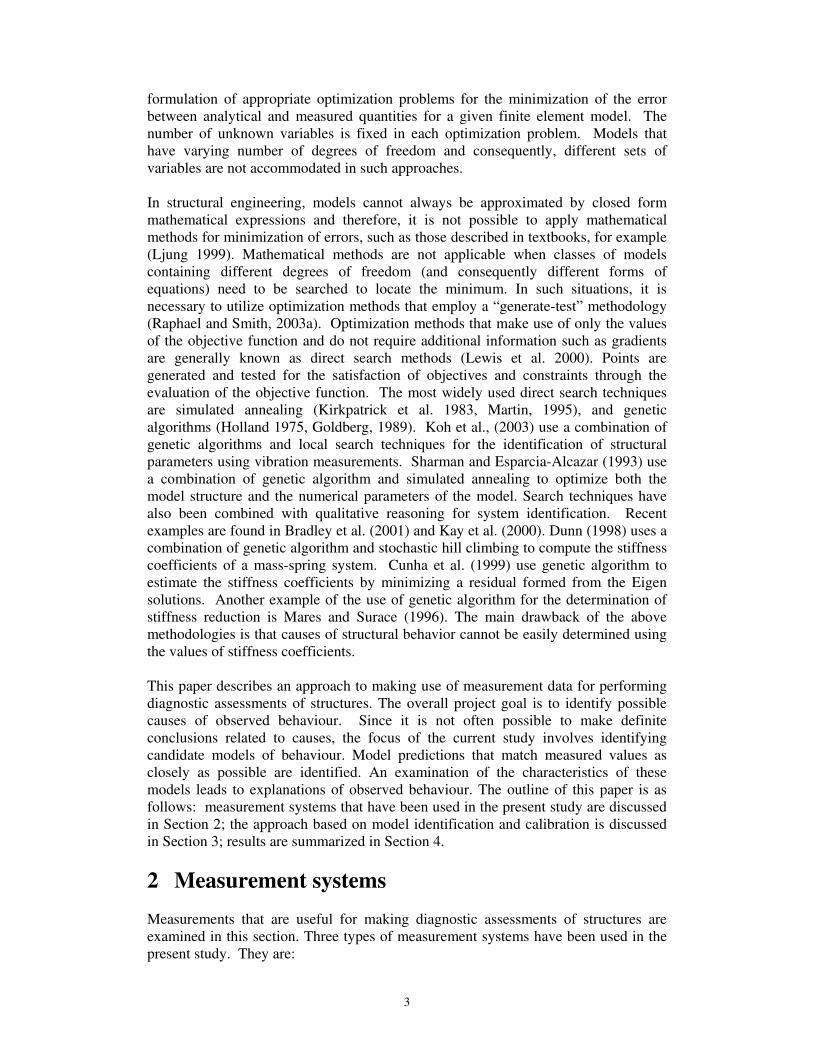
The simplest approach consists of fitting a polynomial through the measured values.

Three inclinometers define a second order polynomial. Higher order polynomials can

be fitted with more inclinometers. By integrating the polynomial, and applying the

boundary conditions, the deflected shape is obtained. Even though reconstruction of

the deflected shape by simple polynomials has been found to be effective, its practical

application is difficult due to sensitivity to measurement errors since the polynomial is

forced to pass through all the measured values. Least squares fit might be used to

reduce the sensitivity to measurement errors. However results are unlikely to be

accurate since theoretical deflections for structures with continuously varying cross

section properties cannot be described by simple functions.

Considering these weaknesses another approach was used. Deflected shapes are

reconstructed by means of linear combinations of a series of pre-calculated deflected

shapes (Burdet and Zanella, 2000). Structures deflect following smooth “engineer’s

curves” under standard load cases (Figure 2). A linear combination of a certain

number of these curves, yields a curve that is also a smooth curve. Each deflected

shape respects the bridge properties, and can account for discontinuities, such as

sudden changes of inertia, much better than polynomials.

Figure 3 shows the deflected shape that is reconstructed using pre-calculated deflected

shapes (base shapes). Also shown in the figure is the shape that is obtained by

integrating a fourth degree polynomial and applying the boundary condition that there

are no displacements at both supports. Both curves lie close to deflection data that are

measured directly.

A feature of the method of using precalculated deflected shapes is that the

reconstructed deflected shape yields additional information on the way the best

6

deflected shape is obtained. For example, a case where all combinations of two of the

four loading patterns of Figure 2 are used, the combination that gives the best result is

10% of uniform loading plus 102% of unit load at 0.75 L, where L is the span. The

interpretation of these coefficients, and their variation over time provides additional

information about the behavior of the bridge. It is for example expected that

significant changes in the structure will lead to significantly different factors used in

the controlling combination, thus indicating that the structure has changed.

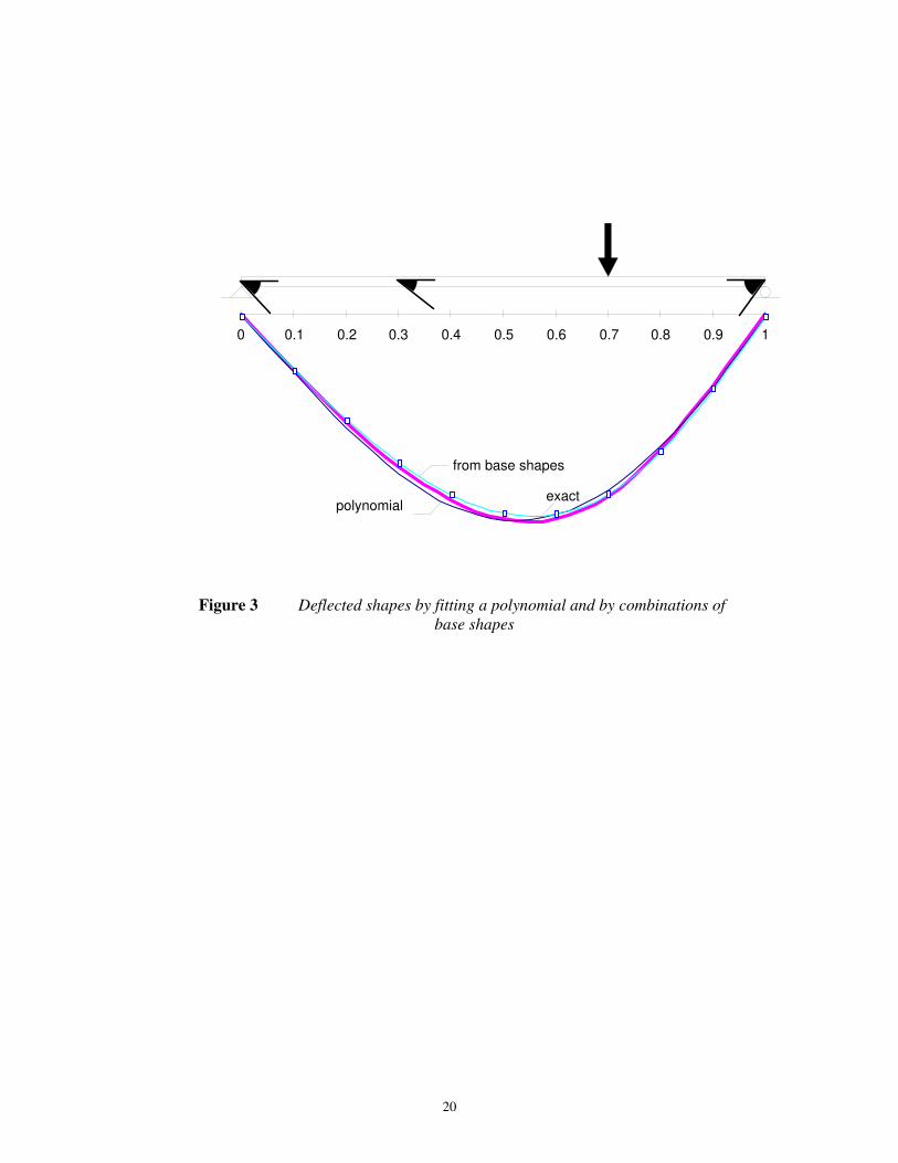
Results obtained by applying this procedure to inclinometer measurements taken

during a load test on Lutrive bridge (See Section 3.1) are shown in Figure 4.

Computed deflections have a good match with those that are directly measured using

optical leveling instruments.

2.3 Fibre optic sensors (SOFO)

The SOFO (Surveillance d’Ouvrage par Fibre Optique) system is based on low

coherence interferometry in standard optical fibres that are used in telecommunication

(Inaudi et al. 1994). The system measures small deformations and provides a

resolution of approximately 2 microns. A significant advantage of the system

compared with conventional strain gauges is that long gauge lengths are possible and

therefore, local effects such as cracking do not influence measurements. Also, since

the system uses light rather than electricity, long term absolute measurements are

more reliable. The system has been successfully installed in many bridges.

Internal deformations are difficult to interpret. Therefore, the deflected shape of

bridged are computed from internal deformations measured by SOFO sensors through

the following procedure (Vurpillot et al., 1998):

• The bending curvature is computed from strain measurements assuming that

plane sections remain plane after bending (Bernoulli beam hypothesis). If two

fibre optical sensors are placed on the upper part and lower parts of a beam

element, the curvature is computed using this relationship:

1

supinf

r

1

lY

ll

m ⋅

−= (1)

where,

rm is the mean radius of curvature

l1 is the initial length of upper and lower sensors

l sup is the final length of upper sensor

l inf is the final length of lower sensor

Y is the distance between upper and lower sensors

• The curvature is integrated twice and appropriate boundary conditions are

applied to obtain the deflected shape.

Figure 5 shows a comparison between the deflection shape retrieved using this

procedure and direct measurements using strain gauges.

3 Model identification and calibration

7

Currently, measurements are mostly used for continuously monitoring deflections in

order to detect changes in structural behavior. In this work, measurements are used to

improve understanding of the behavior of the structure. A strategy that makes use of

measurements to improve model identification and calibration is described in this

section.

The main objective of this study is to identify characteristics of behavior models that

result in measured responses. Unlike recent work on model updating, the goal is not

to find values of stiffness coefficients that produce measured responses. Instead, we

are interested in identifying reasons for structural behavior such as support

settlements and cracks. Sets of models are searched and sets of parameter values are

computed such that the residual errors between predictions and measurements are

minimized.

The fundamental strategy is “generate and test” as described in Section 1. Most

importantly, this strategy involves searching among diverse models that have varying

number of degrees of freedom and do not have explicit closed form mathematical

expressions for responses. A search algorithm called PGSL (Probabilistic Global

Search, Lausanne) (Raphael and Smith, 2003b) was used for finding sets of

combinations of values of model parameters that produce close matches to

measurements. PGSL performs global search by sampling the solution space using a

probability density function (PDF). At the beginning of search, a uniform PDF is

assumed for the entire search space so that solutions are generated purely randomly.

When good solutions are found, probabilities in those regions are increased so that

more intense sampling is carried out in the neighborhood of good solutions. The key

assumption is that better sets of points are found in the neighborhood of good sets of

points. The search space is gradually narrowed down so that convergence is achieved.

The PGSL algorithm includes four nested cycles (Figure 6a):

• Sampling cycle

• Probability updating cycle

• Focusing cycle

• Subdomain cycle

In the sampling cycle (innermost cycle) a certain number of samples, NS, are

generated randomly according to the current PDF. Each point is evaluated by the

user-defined objective function and the best point is selected. In the next cycle,

probabilities of regions containing good solutions are increased and probabilities

decreased in regions containing less attractive solutions (Figure 6b). In the third cycle,

search is focused on the interval containing the best solution after a number of

probability updating cycles, by further subdivision of the interval (Figure 6c). In the

subdomain cycle, the search space is progressively narrowed by selecting a

subdomain of smaller size centred on the best point after each focusing cycle. This is

done by multiplying the current width of each axis by a scale factor.

8

During model calibration, PGSL minimizes the root mean square error (RMSE),

which is calculated using the following equation:

n

xx

RMSE i

mici∑ −=

2

,, )(

(2)

where xi,m is the value measured at the i-th measurement point and xi,c is the

corresponding value computed using the model. The search routine identifies

combinations of values of model parameters that produce low values of RMSE. Since

PGSL is based on global sampling there is no need to provide initial values to search

variables. Bounds of variables are specified based on engineer’s expectations of

possible variations in values.

As an alternative to the procedures described in Sections 2.2.1 and 2.3, models once

calibrated may be employed to compute deflected shapes from measured slopes and

internal deformations. First, candidate models are identified in which predicted

slopes and strains match measurements. Next, these models are analyzed to obtain

the deflected shape. Through this procedure, assumptions related to the degree of

polynomial need not be made and the deflected shapes conform to the laws of

structural mechanics.

The Lutrive bridge example is taken next to illustrate the model identification and

calibration strategy. The measurement event that is evaluated is a load test that was

conducted in 1997. The advantage of this case is that knowledge of the loading,

including magnitude and position on the structure, is available.

3.1 Lutrive Bridge

The Lutrive highway bridge was constructed in 1972 using the cantilever method with

central hinges (articulations). Two bridges, (North and South Lutrive bridges) were

built (one for each direction of traffic) with a length of 395 m. each and a maximum

span of approximately 130 m. The longitudinal section is shown in Figure 7. The

cross-section of the bridge is a pre-stressed box-girder with variable inertia. The

maximum height is 8.50 m. at the column and 2.50 m. in the mid-span, at the hinges.

At the location of the hinge, the deck is reduced to 0.14m, without interrupting the

continuity of the beam (Figure 7c). More information about the bridge can be found

in [Burdet and Badoux, 1999]. A brief history of the bridge is given below:

1971-1972 Construction of the bridge

1973, 77, 78, 80, 85, 86 Annual optical level meter measurements

1986 An engineering office was given the contract to survey

the bridge after large deformations were observed at mid-

span

December 1988 External pre-stress is added to the two bridges

1988-1999 Displacement on the south bridge increases. New

measurement systems are installed on both bridges,

including a hydrostatic leveling system (1988), and fiber

optical sensors (1996)

November 1997 Load tests with fiber optic sensors, inclinometers, and

9

optical level meter

December 1999 New additional external pre-stress added to the south

bridge

3.2 Load tests on Lutrive bridge

Finding a good explanation for abnormal increases in deflections in the Lutrive bridge

has remained a challenge for several years. Various hypotheses involving parameters

such as creep, pre-stress and models of joints at mid-span have been made. In order to

improve understanding of the behavior of the bridge and to find out causes for

abnormal deflections, load tests were carried out on the bridge in 1997.

One section of the bridge was equipped with instruments (Figure 7a). During the load

test, a truck was placed on the part of the bridge that was instrumented in order to

produce maximum deflections at the locations of sensors. The weight of the truck

was approximated to be a two-point load placed non-symmetrically (Figure 7b).

3.2.1 Measurement system

The following measurement systems were used during the load tests.

• Fiber optic sensors at the following five longitudinal positions (Perregeaux

1998) from the column in the Lausanne direction:

8.4m., 20.4 m., 32.5 m., 44.5 m., 56.8 m.

• Inclinometers at four positions from the same column (Burdet and Fleury,

1997):

16.1 m., 29.5 m., 49.3 m., 65.75 m.

• Optical level meters at four positions from the same column

(Burdet and Fleury, 1997):

11.9 m., 29.9 m., 47.8 m., 65.75 m.

The following measurement data are obtained from the measurement systems:

• Deformations of sensors placed on the top and bottom of the bridge define the

bending curvature.

• Inclinometers give the slope of the cross-section.

• Optical level meters give the vertical displacement of cross-sections.

3.3 Model identification

Initially, simple models were used to interpret the measurements from load tests.

When simple models were found to be inadequate to explain the results, more

complex models containing additional variables were created. Values of selected

variables were determined through identifying low values of the root mean square

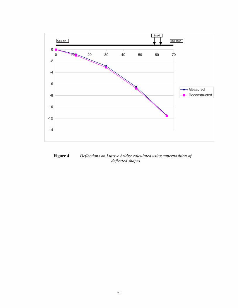
error, see Equation 2. A sample set of models are discussed next. Only the part of the

bridge from the column to the mid-span (the part that was equipped with

measurement instruments) was modeled with models A, B, C, and D (Figure 8). The

complete bridge excluding the columns was modeled using E.

10

Even though, PGSL is able to search automatically among classes of models that have

varying numbers of degrees of freedom, in this work, model classes are manually

selected and PGSL is used only for estimating values of parameters. The goal is to

study the capability of each model class to explain measured data. Variables have

been chosen such that there is a unique global minimum for each model class within

specified variable bounds and the current study is not affected by the influence of

local minima.

3.3.1 A sample set of models

3.3.1.1 Model A: Cantilever

This is a simple model that was used in a previous study (Perregeaux, 1998). The

objective of using this model is to evaluate the boundary case of a cantilever bridge

using expected values of material properties. It was assumed that there is no shear and

moment transfer through the hinge from the other side. The structural system is a

cantilever with parabolic section profile (variable moment of inertia). The value of

Young’s modulus (E) is taken to be 38e6 kN/m2. Since there were no unknown

variables, no calibration was used and the structure was evaluated analytically. This

model did not achieve an acceptable correlation with measurements. There was more

than 200% error in the mid-span deflection.

3.3.1.2 Model B: Propped cantilever

In order to investigate the effect of shear transfer from the other side of the hinge, a

propped cantilever model was used in which a spring is used to support the beam at

the propped end. The stiffness of the spring was estimated to be 17’114 kN/m. No

calibration was used since all the parameters were assigned constant values. This

model produced a close match with measured deflections. However, predictions of

curvatures did not match the measurements.

3.3.1.3 Model C: Beam with springs

Since the predictions of curvature using model B did not match measured values, it

was suspected that the bending moments in the beam did not correspond to what was

predicted using a propped cantilever model. Therefore, additional springs were added

to adjust the boundary conditions of the model. Specifically, a horizontal spring was

added at the midspan to model the arch effect caused by the variation in the position

of the neutral axis. The spring stiffnesses were considered to be variables and

possible values were identified using PGSL. Three separate searches were carried out

to minimize the RMSE between predicted and observed deflections, slopes and

curvatures respectively. The search using measured deflections produced a good

match with respect to deflections. However, the calibrated model did not produce

matching slope or curvature. Similarly, minimization of RMSE in slopes and

curvatures did not produce a good match with respect to measurements that were not

used in the calibration. The values of variables determined through this strategy are

given in Table 1.

11

3.3.1.4 Model D: Beam supported on springs with rigid body rotation

When Model C was calibrated using curvature measurements, slopes were found to

differ from measured values by a constant value. Therefore, a variable representing

rigid body rotation at the left support was added to the model. Variables of this model

were then determined through minimizing the RMSE in slope. The values of these

variables are given in Table 1. There is a good match with deflections even though

deflection measurements were not used in the calibration. Since possible explanations

for the rigid body rotation (-0.072) could not be accepted this model was discarded.

Values of variables in the model found by PGSL Model Measurements

used for

calibration E

[kN/m2]

k

[kN/m]

k1

[kNm/rad]

k2

[kN/m] θrig

[mrad]

C deflection 50.00e6 28’076 9.99e19 2.8e-8 -

C slope 28.34e6 15’625 9.96e19 2.64e-4 -

C curvature 48.64e6 16’300 9.81e19 5.48 e5 -

D curvature 48.64e6 16’300 9.81e19 5.48 e5 -0.072

Table 1: Model parameters determined by optimization

3.3.1.5 Model E: Finite element model of the entire structure

Examination of model D made it clear that boundary conditions are important.

Therefore, the entire structure was modeled and analyzed using finite element

method. Since models C and D highlighted the importance of varying the position of

the neutral axis in order to produce an arch effect, (especially at the location of the

hinge), this feature was included in the model. The hinge was modeled using a beam

element with reduced value of the stiffness. The Young’s modulus of concrete was

calibrated in order to produce a good match with measurements. The final value

obtained is 30e6 kN/m2. This model produced good match with deflections and

reasonable match with slope and curvature. Therefore, this is the most attractive

candidate model found in this study.

3.3.2 Summary of results

Values of displacement, slope and curvature that are predicted by models and

measured on the structure are shown in Figures 9-11. Each curve shows the prediction

of a candidate model along the length of the beam and is obtained be interpolating

values computed at measurement points. For finite element models, values are

computed at gauss points nearest to measurement points.

3.3.3 Analysis of results

The results are used to classify models based on the percentage deviation (PD) which

is computed by dividing the root mean square error by the mean value of data points.

12

Models are classified as good (PD <25%), reasonable (PD 25-50 %) and bad (PD >

50 %) as shown in Table 2.

Model Criteria

Measurement used for calibration

is given in brackets

Displacement Slope Curvature

A Bad - -

B Good Reasonable Bad

C (deflection) Good Bad Reasonable

C (slope) Bad Good Reasonable

C (curvature) Bad Reasonable Good

D (curvature) Good Good Good

E Good Reasonable Reasonable

Table 2: Evaluation of models

The following observations are made from this study:

• Selecting models through reference to only one type of observation is not

sufficient. It is easy to obtain models whose variable values provide a close

match with one type of measurement through the model calibration strategy.

However, these models may not be compatible with other types of

measurements.

• When finite element models are used, a small change in boundary conditions

greatly affects the results. When Model E was modified such that the hinge

position coincides with the neutral axis, results were not satisfactory and

therefore, they are not presented in this paper.

• The process of identifying models that are compatible with measurements may

lead to examining models that have large numbers of variables. Model D

contained 5 variables. The number of observation points must be greater than

the number of parameters. A better match with more parameters does not

necessarily mean that the quality of the model is better.

• Model calibration is useful for validating models as well as filtering out bad

models. For example, Model C did not give good results for all three types of

calibration attempts.

• Curvature data measurements show a change in sign near the hinge indicating

that the mid-span joint transfers shear stress. This is not possible with Model

A.

• Quantitative information related to values of parameters is more difficult to

verify: For instance, Young Modulus of Model E is 30e6 kN/m2 whereas it is

48.6e6 kN/m2 for Model D.

• Models can only be accepted if sound physical explanation is found. Even

though Model D resulted in a good match with all types of measurements, it

was not accepted because a physical explanation could not be found for the

calibrated value of rigid body rotation.

Predictions of Model E match well with all measurements. Model E is equivalent to

Model D within the part of the bridge that is instrumented since for Model E, spring

stiffnesses and rotations are influenced by other parts of the bridge. However, model

E does not involve arbitrary stiffness coefficients and rigid body rotations as does

13

model D. Correct modeling of the hinge is necessary to produce good predictions; the

location of the hinge should be above the neutral axis of the beam and the hinge

should be capable of transferring both horizontal and vertical forces. Mid span

deflection may more than double if the hinge is incapable of transferring these forces.

Therefore, it is hypothesized that hinge characteristics have changed over time in the

Lutrive bridge and this has caused mid span deflections to increase.

4 Summary and conclusions

The following conclusions are drawn from this study:

• Measurements of deflections, rotations and internal deformations in concrete

structures are now more reliable with the development of new equipment such

as fibre optic sensors and inclinometers. Periodic monitoring allows detection

of abnormalities. However, model identification techniques are needed for

determining likely causes of abnormalities.

• It is possible to compute deflections from measured rotations and internal

deformations. Thus, one type of measurement may be validated through the

use of other types of independent measurements. Techniques that are

available for computing the deflected shapes from rotations and internal

deformations include integration of approximate polynomials, superposition of

deflected curves and model calibration.

• Model calibration techniques lead to identification of good candidate models.

• Models that are identified through calibration have to be carefully studied by

engineers in order to determine whether they are physically possible. All

models should have sound physical support. When physical justifications

cannot be found, models should be rejected. Alternately, further observations

could reveal sufficient support for some candidate models.

• PGSL is an effective global search algorithm for model calibration tasks. In

all the models of Lutrive bridge that were considered, PGSL was able to find

parameter values that predicted a good match with the measurement data that

was used in calibration.

• A plausible explanation for the increased deflection of the Lutrive bridge is a

change in centre span hinge characteristics.

Further work is necessary to determine the mechanisms which have lead to changes in

hinge characteristics. Possible explanations involved plasticity induced by prestress

and subsequent stress cycles due to temperature variations.

This work has already been extended to search among multiple model classes using

PGSL for system identification. A study of the reliability of system identification

using this procedure is also in progress.

References

Abe M. (1998), Vibration control of structures with closely spaced frequencies by a

single actuator, Journal of Vibration and Acoustics, Transactions of the American

Society of Mechanical Engineers, Vol.120, pp.117-124.

14

Banan M.R., Banan M.R., and Hjelmstad K.D. (1994a), Parameter estimation of

structures from static response. Part 1. Computational aspects, Journal of structural

engineering, ASCE, 120(11), pp. 3243-3258.

Banan M.R., Banan M.R., and Hjelmstad K.D. (1994b), Parameter estimation of

structures from static response. Part 2. Numerical simulation studies, Journal of

structural engineering, ASCE, 120(11), pp. 3243-3258.

Beck J.L. and Katafygiotis L.S. (1998), Updating Models and Their Uncertainties. I:

Bayesian statistical framework, Journal of Engineering. Mechanics. 124, pp. 455-461.

Brownjohn J.M.W, Moyo P., Omenzetter P., Lu Y. (2003), Assessment of highway

bridge upgrading by testing and finite-element model updating. Journal of bridge

engineering, ASCE, 37, pp. 162-172.

Bradley E., Easley M., and Stolle R. (2001), "Reasoning about nonlinear system

identification," Artificial Intelligence, 133:139-188.

BURDET O. (1993), Load Testing and Monitoring of Swiss Bridges, Comité

Européen du Béton, Safety and Performance Concepts, Bulletin d'information n°219,

Lausanne, Suisse.

Burdet O. and Badoux M.,(1999), Long-term Deflection Monitoring of Prestressed

Concrete Bridges Retrofitted by External Post-Tensioning - Examples from

Switzerland, IABSE Symposium "Structures for the Future - The Search for Quality",

Rio de Janeiro, Report Vol 83, pp.112-114.

Burdet O., Fleury B. (1997), Pont sur la Lutrive aval (VD)- Rapport d’essai de charge

statique complémentaire, EPFL-IBAP.

Burdet O., Zanella J.-L. (2000), Automatic Monitoring of Bridges using Electronic

Inclinometers, IABSE, , Lucerne Congress Structural Engineering for Meeting Urban

Transportation Challenges, pp. 398-399, Zürich, Switzerland, September.

Castello D.A., Stutz L.T., Rochinha F.A. (2002), A structural defect identification

approach based on a continuum damage model, Computers and structures, 80, pp.

417-436.

Chaudhary M.T.A., Abe M, Fujino Y., and Yoshida J. (2000), Performance evaluation

of two base-isolated bridges using seismic data, Journal of Structural Engineering,

ASCE, Vol.116, No.10, pp.1187-1195.

Cunha J., Cogan S., Berthod C. (1999), Application of genetic algorithms for the

identification of elastic constants of composite materials from dynamic tests,

International Journal for Numerical Methods in Engineering, 45, 7, pp. 891-900.

Daverio R. (1995), Mesures des déformations des ponts par un système

d'inclinométrie, Rapport de maîtrise EPFL-IBAP, Lausanne, Switzerland.

15

Dunn S. A. (1998), The use of genetic algorithms and stochastic hill-climbing in

dynamic finite element model identification, Computers & Structures, 66, 4, pp. 489-

497

Favre R., Burdet O., Charif H., Hassan M., Markey I.F. (1995), Enseignements tirés

d'essais de charge et d'observations à long terme pour l'évaluation des ponts en béton

et le choix de la précontrainte, Office Fédéral des Routes, recherche 83/90, Suisse.

Fest E. (1997), Système de mesure par inclinométrie: développement d'un algorithme

de calcul des flèches, DEA Ecole Normale supérieur de Cachan, France.

Friswell M.I. and Mottershead J.E. (1995), Finite element model updating in

structural dynamics, Kluwer.

Goldberg, D.E. (1989), Genetic Algorithms in Search, Optimization, and Machine

Learning, Addison-Wesley, Reading, MA.

Hajela P. and Soeiro F. J. (1990), Structural damage detection based on static and

modal analysis," AIAA Journal, Vol. 28, No. 6, pp 1110 – 1115.

Hemez F.M., Doebling S.W. (2001), Review and assessment of model updating for

non-linear, tansient dynamics, Mechanical Systems and Signal Processing, Vol 15(1),

pp.45-74.

Holland J. (1975), Adaptation in natural artificial systems, University of Michigan

Press.

Hjelmstad K.D., and Shin S. (1997), Damage detection and assessment of structures

from static response, Journal of Engineering Mechanics, pp. 568-576.

Housner G. W., Bergman L. A., Caughey T. K., Chassiakos A. G., Claus R. O., Masri

S. F., Skeleton R. E., Soong T. T., Spencer B. F., and Yao J. T. P. (1997), Structural

control: past, present, and future, Journal of Engineering Mechanics, ASCE, Vol.

123(9), pp. 897-972.

Hu N., Wang X., Fukunaga H., Yao Z.H., Zhang H.X. and Wu Z.S. (2001), Damage

assessment of structures using modal test data, International Journal of Solids and

Structures, 38, pp. 3111-3126.

Inaudi D., Elamarib A., Pflug L., Gisinb N., Breguetb J., Vurpillot S. (1994), Low-

coherence deformation sensors for the monitoring of civil-engineering structures,

Sensors and Actuators A 44, pp. 125-130.

Katafygiotis L.S. and. Beck J.L. (1998), Updating models and their uncertainties. II:

model identifiability, Journal of Engineering Mechanics, 124, pp. 463-467.

Kay H., Rinner B., and Kuipers B. (2000). Semi-quantitative system identification.

Artificial Intelligence, 119, pp. 103-140.

16

Kirkpatrick, S., Gelatt C. and Vecchi M. (1983). Optimization by simulated

annealing, Science, pp. 220:673.

Koh C.G., Chen Y.F., Liaw C.-Y. (2003), A hybrid computational strategy for

identification of structural parameters, Computers and Structures, 81, pp. 107–117.

Liu P. and Chian C. (1997), Parametric identification of truss structures using static

strains, ASCE Journal of Structural Engineering, July 1997, 123, 7, pp. 927-933.

Lewis, R.M., Torczon, V. and Trosset, M.W. (2000), Direct search methods: then and

now, Journal of Computational and Applied Mathematics, 124, 191–207.

Ljung L. (1999), System Identification - Theory For the User, Prentice Hall.

Mares, C., Surace, C. (1996), Application of genetic algorithms to identify damage in

elastic structures, Journal of Sound and Vibration, 195, 2, pp. 195-215.

Martin O. (1995), Combining simulated annealing with local search heuristics,

Metaheuristics in combinatoric optimization, (G.Laporte and I.Osman editors).

Modak S.V., Kundra T.K., Nakra B.C. (2002), Comparative study of model updating

studies using simulated experimental data, Computers and Structures, 80, pp. 437-

447.

Park K.C. and Felippa, C.A. (2001), A flexibility-based inverse algorithm for

identification of structural joint properties, In Proceedings of ASME symposium on

computational methods on inverse problems, 15-20 November 1998, Anaheim, CA.

Perregeaux N. (1998), Pont de la Lutrive-N9, Equipement et analyse du

comportement au moyen du système de mesure à fibre optique SOFO, Diploma

Thesis, EPF-Lausanne.

Perregaux N., Vurpillot S., Tosco J-S., Inaudi D., Burdet O. (1998), Vertical

displacement of bridges using the sofo system: a fiber optic monitoring method for

structures, ASCE-12th Engineering Mechanics. Conference Proceedings: A force for

the 21st Century, 791-794, San Diego, USA,.

Raphael B. and Smith I.F.C. (2003a), Fundamentals of computer aided engineering,

John Wiley, UK.

Raphael B. and Smith I.F.C. (2003b), “A direct stochastic algorithm for global

search”, J of Applied Mathematics and Computation, Vol 146, No 2-3, pp 729-758.

Reich, G. W. and Park, K. C. (2001), A theory for strain-based structural system

identification, Journal of Applied Mechanics, 68(4), 521-527.

Sohn H., and Law K.H. (1997), A Bayesian probabilistic approach for structural

damage detection, Earthquake engineering and structural dynamics, 26, PP. 1259-

1281.

17

Sohn H., and Law K.H. (2001), “Damage diagnosis using experimental ritz vectors,”

Journal of Engineering Mechanics, ASCE, Vol. 127, No. 11, pp. 1184-1193.

Sanayei, M., and Onipede, O. (1991), "Damage assessment of structures using static

test data," AIAA Journal, Vol.29, No.7, pp.1174-1179.

Sanayei, M., and Scampoli, S. (1991), "Structural element stiffness identification

from static test data," Journal of Engineering Mechanics, ASCE, pp. 1021-1036.

Sanayei, M., and Saletnik, M. J. (1996), "Parameter estimation of structures from

static strain measurements; I: formulation," Journal of Structural Engineering, ASCE,

Vol. 122, No. 5, pp. 555-562.

Sanayei, M., and Saletnik, M. J. (1996), "Parameter estimation of structures from

static strain measurements. II: error sensitivity analysis," Journal of Structural

Engineering, ASCE, Vol. 122, No. 5, pp. 563-572.

Teughels A., Maeck J., Roeck G. (2002), Damage assessment by FE model updating

using damage functions, Computers and structures, 80, pp. 1869-1879.

Yu L., Law S.S., Link M., Zhang L.M. (1999), damage detection in bolted joint

structures using element contribution to modal strain energy, In Proceedings of the

Second International Conference on Identification in Engineering Systems, Swansea,

M.I. Friswell, J.E. Mottershead and A.W. Lees (eds.), pp. 516-526,.

Vurpillot S., Krueger G., Benouaich D., Clément D., Inaudi D. (1998), "Vertical

deflection of a pre-stressed concrete bridge obtained using deformation sensors and

inclinometer measurements", ACI Structural Journal, Vol 95, No 5, p 518 - 526.

Wyler AG. (1996), Technical specifications for Zerotronic Inclinometers, Winterthur,

Switzerland.

18

Figure 1 Simple support for a fixed inclinometer

19

Figure 2 Load cases used for the pre-calculation of the base shapes

0.25 0.5 0.75

inclinometers

20

Figure 3 Deflected shapes by fitting a polynomial and by combinations of

base shapes

0 0.1 0.2 0.3 0.4 0.5 0.6 0.7 0.8 0.9 1

exact

from base shapes

polynomialy( ) = 0l

21

-14

-12

-10

-8

-6

-4

-2

0

0 10 20 30 40 50 60 70

Measured

Reconstructed

Mid-spanColumn

Load

Figure 4 Deflections on Lutrive bridge calculated using superposition of

deflected shapes

22

Figure 5 Comparison between vertical deflection retrieved from SOFO

measurements and those measured by dial gauges (Vurpillot et al. 1998).

23

a) Nested cycles in PGSL. NSDC, NFC, NPUC and NS are the number of iterations

in the subdomain, focusing, probability updating and sampling cycles respectively.

b) Evolution of the PDF of a variable after several focusing cycles.

c) Changing the sub-domain after each subdomain cycle.

Figure 6 PGSL

Sub-domain cycle

Focusing cycle

Probability updating cycle

Sampling cycle

repeat NSDC times

repeat NFC times

repeat NPUC times

Evaluate NS samples

x xmin xmax

Cycle 1

Cycle 2

Cycle 3

Cycle 4

Cycle 5

Best points in each cycle

24

a. Longitudinal section of Lutrive Bridge (values in meters)

~1.70 ~3.80 ~2.00

VeveyLausanne

6 kN 19 kN

b. Load test on the bridge

3 m

2 x 2 cables VSL type Z 6-18

Barres DYWIDAG Ø15cable VSL 5-7

2.5 m

0.3 m

c. Details of the hinge

Figure 7 Lutrive Bridge

Section equipped with measurement instruments

25

Figure 8 Sample set of models examined for the example of the Lutrive

bridge

26

0.00

5.00

10.00

15.00

20.00

25.00

30.00

35.00

0 10 20 30 40 50 60 70

position [m]

dis

pla

cem

ent

[mm

]

A

B

C (opt. deflection)

C (opt. slope)

C (opt. curvature)

D

E

data measurement

Mid-span

Column

Load test

Figure 9 Measured and predicted deflections

27

-1.00E-05

-8.00E-06

-6.00E-06

-4.00E-06

-2.00E-06

0.00E+00

2.00E-06

4.00E-06

6.00E-06

8.00E-06

1.00E-05

0 10 20 30 40 50 60 70position [m]

cu

rva

ture

[1

/m]

B

C (opt. deflection)

C (opt. slope)

C (opt. curvature)

D

E

data measurement

Mid-spanColumn Load test

Figure 10 Measured and predicted curvatures

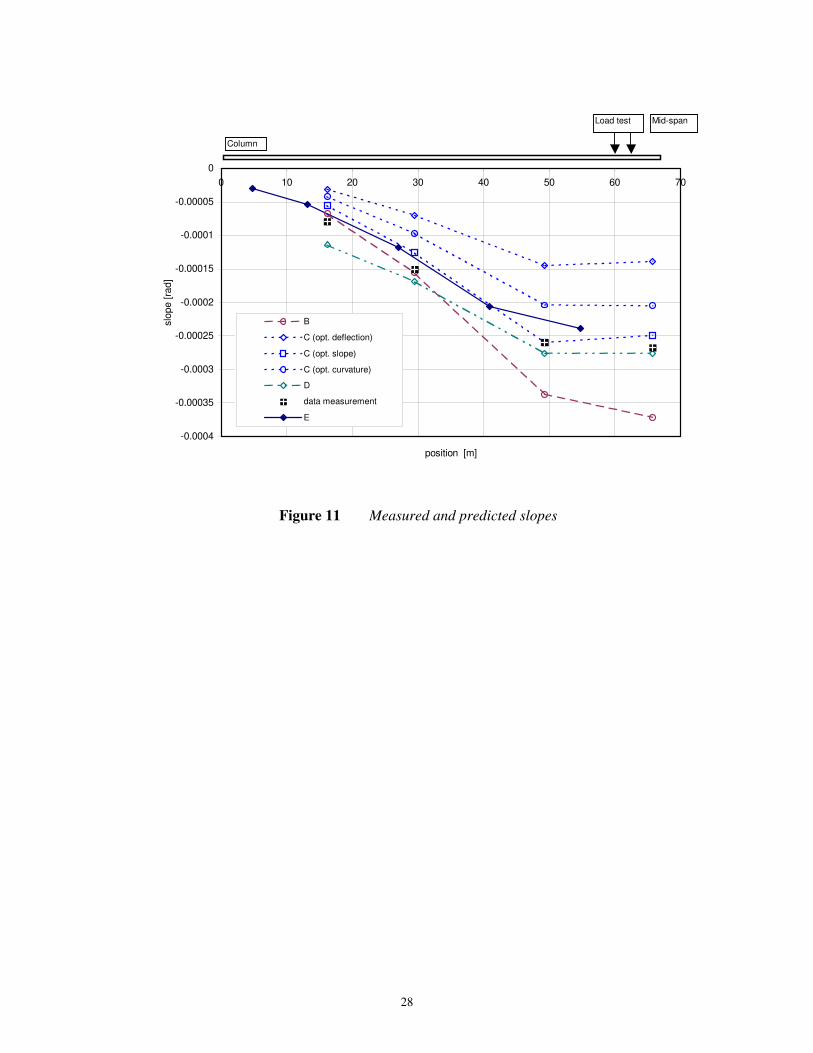
28

-0.0004

-0.00035

-0.0003

-0.00025

-0.0002

-0.00015

-0.0001

-0.00005

0

0 10 20 30 40 50 60 70

position [m]

slo

pe [

rad]

B

C (opt. deflection)

C (opt. slope)

C (opt. curvature)

D

data measurement

E

Mid-span

Column

Load test

Figure 11 Measured and predicted slopes