Embed Size (px)
Citation preview

1
RADIO FREQUENCY IDENTIFICATION FOR
THE MEASUREMENT OF OVERHEAD POWER
TRANSMISSION LINE CONDUCTOR SAG
BY
TLOTLOLLO SIDWELL HLALELE
SUBMITTED IN ACCORDANCE WITH THE
REQUIREMENTS FOR THE DEGREE OF
(MASTER OF TECHNOLOGY)
IN
ELECTRICAL ENGINEERING
AT THE
UNIVERSITY OF SOUTH AFRICA
SUPERVISOR: PROF S DU
17 July 2015

2
DECLARATION OF OWN WORK
I (…………………………………………) declare that the dissertation entitled, “Employ radio
frequency identification to the measurement of overhead power transmission line conductor sag” is
my own work and that all the sources that I have used or quoted have been indicated and
acknowledged by means of complete reference.
Signature of student:………………………… Date:………………………….
Student number:………………………………
Signature of Supervisor:……………………… Date:………………………….

3
ACKNOWLEDGEMENTS
I would like to express my gratitude to my supervisor Prof. Shengzhi Du for his support,
inspiration and encouragement throughout the entire work.
List of Acronyms

4
AM -amplitude modulation
FM- frequency modulation
JDBC- Java database connector
RFID- radio frequency identification
OHTL -overhead transmission line
GPS- global position system
MRS -Magneto resistive sensors
PLC- power line carrier method
CT- current transformer
VT- voltage transformer
UHF- ultra-high frequency
EMI- electromagnetic interference
NAVSTAR Navigation satellite Timing and ranging
NERSA National Energy regulator South Africa
RMS – Root mean square
PU – Per Unit value
SNR- Signal noise ratio
NF noise figure
RF radio frequency
A cross section area
Apk-pk peak-to-peak galloping amplitude
CD aerodynamic drag coefficient
CL aerodynamic lift coefficient
Δ- Deflection

5
γ- Curve fitting factor defined
DGPS Differential Geographical positioning system
ACSR Aluminum conductor steel reinforced
ACSS Aluminum conductor steel supported
SDC Self damping conductor
VR Vibration resistance
AAC All Aluminum conductors
List of Key words
Conductor sag detection
Power quality
Power reliability
Radio frequency identification
RFID radar system

6
ABSTRACT
This dissertation deals with the challenge of power utility in South Africa which is on proactive
detection of fallen power line conductors and real time sagging measurement together with slipping
of such conductors. Various methods which are currently used for sag detection were characterized
and evaluated to the aim of the research. A mathematical reconstruction done to estimate the lowest
point of the conductor in a span is presented. Practical simulations and application of radio
frequency identification (RFID) for sag detection is attempted through matlab software. RFID
radar system is then analyzed in different modes and found to give precision measurement for sag
in real time as opposed to global positioning system (GPS) if one dimension of the tag assumed
fixed on the power line. Lastly errors detected on the measurements are corrected using a trainable
artificial neural network. A conclusion is made by making recommendations in the advancement
of the research.
PROBLEM STATEMENT
In South Africa, electric utilities such as Eskom are under pressure to make optimum use of their
existing facilities, of which the high voltage power transmission line is the back bone. The current
flowing in the conductors together with the resistance causes losses and local heating, leading to
the linear expansion of the conductors. These result to the conductor sagging. Furthermore,
proactive detection of fallen power lines and real time sagging measurement is very critical in
power transmission. Additional current due to a failure of a parallel route causes more losses and
hence more sagging. When too much sagging occurs there is a potential for a dangerous situation to
develop or a total failure if they touch the ground. A power utility need to accurately measure both

7
electric current and line positions in real time, in order to enable the dynamic rating of the power
networks.
Factors such as mechanical stress, solar radiation, wind speed, conductor geometry, ice force and
ambient temperature causes a problem of torsional motion and the vertical cable deflection, hence
more sagging.
HYPOTHESIS
Radio Frequency Identification system (RFID) technology has a potential of giving an accurate
conductor sag measurement in real time. With narrow bandwidth which allow it not to interfere
with other communication systems at about 915MHz frequency, the angle of arrival measurement
can virtually be used in conjunction with range to give a 3D positioning system from predesigned
measuring locations to determine conductor sag. Considering a single span of a section for
simulations purposes, passive tag attached to a power line can be detected without external power
supplied to it. This makes RFID sag detection system cost effective and more accurate.
DERMACATION OF THE FIELD OF STUDY
The study reviewed other techniques which are currently used by Eskom and other power
companies for Power line detection. It examined the theory of RFID and its practical application in
real time monitoring of conductor sag. Although there is a lot of improvement in RFID, there is
still much more work and research to be done considering the high voltage corona discharge.

8
TABLE OF CONTENTS
Title Page i
Declaration by Student ii
Acknowledgements iii
List of acronyms iv
List of keywords v
Abstract vi
Problem Statement vi
Hypothesis vii
Demarcation of the field of Study vii
CHAPTER 1 INTRODUCTION
1.1 A detailed problem statement 1
1.1.1 Context of the problem 1
1.1.2 Research gap (power quality concept) 4
1.2 Research objectives and questions 5
1.2.1 The objectives of the study 5
1.2.2 Research questions 6
1.3 Approach 6
1.5 Research goal 6
1.5.1 Research contribution 6
1.5 Study overview 7
1.7 Dissertation outline 8
9
CHAPTER 2 LITERATURE REVIEW
2.1 Introduction 10
2.2 Transmission line sagging 10
2.2.1 Power quality disturbances 11
2.2.2 Determination of sag 12
2.2.3 Level spans 13
2.2.4 Conductor length 15
2.2.5 Wind loading on overhead lines 19
2.2.6 Maximum conductor tension 19
2.2.7 Thermal elongation 20
2.2.8 The occurrence of galloping to sag 21
2.3 Different methods used to measure conductor sag 25
2.3.1 Current transformers 25
2.3.2 Power line carrier method 26
2.3.3 Power donut 29
2.3.4 Global positioning system 31
2.3.5 Image processing based on camera 33
2.3.6 Electro-magnetic coupling method 34
2.3.7 Mathematical approach 35
2.3.8 Magneto resistive sensors 38
2.3.9 Autonomous robot technique 38
2.4 Background of Radio Frequency Identification (RFID) 39
2.4.1 The key parameters of RFID 39
2.4.2 Constraints on Interrogator sensitivity 43
2.4.3 The system throughput 46

10
2.4.4 Data modulation 46
2.4.5 Channel sharing 46
2.4.6 Interrogator interference 47
2.4.7 Tag interference 48
2.4.8 Conclusion 49
CHAPTER 3 THE SYSTEM STRUCTURE DESIGN
3.1 Transmission line performance and sag detection 51
3.2 RFID sag detection and monitoring system 66
3.2.1 Structure design of the monitoring system 67
3.2.2 Principle of the monitoring system 70
3.2.3 Selection of tags 74
3.2.4 Backscattering of the system 76
3.2.5 Interference problem 77
3.2.6 Effect of mounting the antenna 80
3.2.7 Effect of attaching the tag on the conducting materials 82
3.2.8 RFID tag positioning in three dimensions 87
3.2.9 Triangulation Method 89
3.3 Evaluation of the proposed RFID sag monitoring system 95
CHAPTER 4 ANALYSIS AND RESULTS
4.1 The general discussion of RFID system 98

11
CHAPTER 5 CONCLUSION AND DISCUSSION
5.1 Discussion 118
5.2 Conclusion 119
Appendix A: List of publications
Appendix B: Programme code
List of References
12
CHAPTER 1 INTRODUCTION
1.1 A detailed problem statement
Long distance high voltage power lines are very important in electricity power delivery because
power stations are normally built far away from power loads. During the transmission process,
balance must be constantly maintained to match the power supply and demand. Due to the ongoing
electricity needs, existing electrical transmission line performance is also a major concern and a
very critical factor. Electric current and line positions are two important parameters to measure
transmission lines performance. The electric current flowing in the lines should be measured to
avoid overload, phase unbalance and fluctuation. Line positions should be monitored to keep track
of the sagging and galloping situations. In this chapter sagging, galloping, power quality and radio
frequency identification technology are discussed.
1.1.1 Context of the Problem
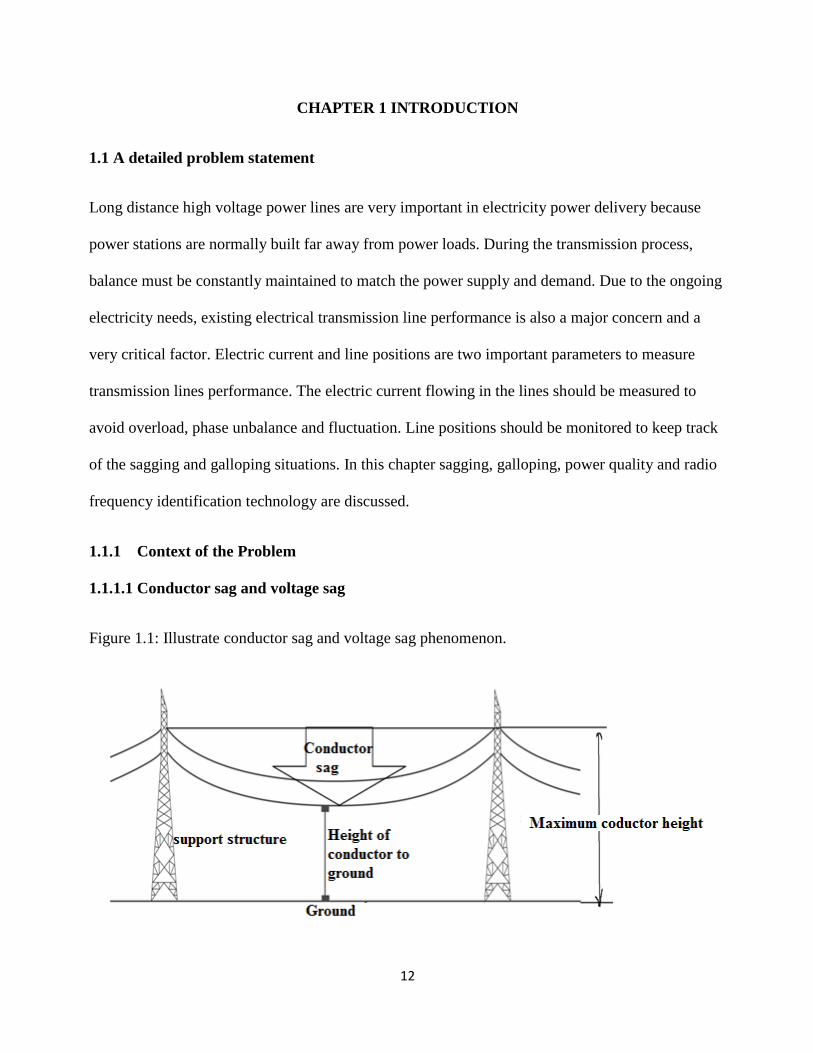
1.1.1.1 Conductor sag and voltage sag
Figure 1.1: Illustrate conductor sag and voltage sag phenomenon.

13
(a) Conductor sag
(b) Voltage sag
Figure 1.1 Conductor sag and voltage sag
Conductor sag is the vertical distance between the point at a maximum height where the conductor
is joined to the tower and the lowest point of the conductor to the ground. It determines electrical
clearances, right of way width, uplift weights, stress and strain, thermal rating. Tension in a form of
force, determines structure angle and dead-end wire load. Tension limits determine conductor’s
system safety factor when calculations are done for design, vibration, and structure cost.
Conductors between two transmission towers often suffer sagging phenomenon. It was reported
that sagging of a conductor in Figure 1.1 (a) can cause a nonlinear power flow in the power system,
which may result in to a sudden reduction in voltage known as voltage sag or voltage dig (IEEE
Standard 1159-1995).

14
According to IEEE Standard 1159-1995 Recommended Practice for Monitoring Electric Power
Quality, voltage sag is a decrease in root mean square (RMS) voltage at the power frequency for
durations from 0.5cycles to 1 minute, reported as the remaining voltage. Conductor sagging can
lower the conductor to an unsafe height above the earth. It can be caused by oscillations which can
result into serious transmission problems, such as flashover due to infringed line-to-line clearance,
risk of mechanical failure of transmission tower, and excessive loading stress. Efforts have been
made to understand this phenomenon better and develop means of protecting the transmission line
against this problem, but there is still a challenge of detecting the sag in real time. The low
frequency, high amplitude induces vibration on this transmission line conductors as a result, causes
serious galloping which result to more sagging.
When the weather is considered, it is valid to interpret galloping as an oscillation of either a single
or bundled conductor due to wind force or wind-induced vibration on an iced or wet snow
accretion on the conductors. It is also caused by steady crosswind acting upon asymmetrically iced
conductor surface. Large amplitude is normally observed on a vertical position depending on the
line construction and the oscillation mode excited.
The cost associated with galloping can be due to damaged components which require inspection
and repair. It damages the conductor strands which result to a conductor’s increase in stress level to
a point of breakage and dynamic overload. In the event of this situation, patrolling need to be
performed to detect any damage. This requires a helicopter or some sort of physical view, which
increase costs and results unplanned maintenance.
The problem of sagging has the impact on system reliability and power quality of service. There
may be a losing of customers who are very sensitive to power quality. There can also be a swinging
of the suspension points longitudinally to the power line which is likely caused by the variation in

15
tension; that could accompany galloping and act to couple the galloping motions in adjacent spans,
resulting to a more dangerous sagging phenomenon.
By constantly tracking the conductor motion, with the distance from this lowest point to the
ground, sag could be proactively measured or determined.
1.1.2 Research gap (power quality concept)
In modern electrical power systems, electricity is produced at generating stations, transmitted
through a high voltage network, and finally distributed to consumers. Due to the rapid increase in
power demand, electrical power systems have been developed extensively during the 21st century,
resulting in today’s power industry probably being the largest and most complex industry in the
world. Electricity is one of the key elements of any economy, industrialized society or country. A
modern power system should provide reliable and uninterrupted services to its customers at a rated
voltage and frequency within constrained variation limits. If the supply quality suffers a reduction
and is outside those constrained limits, sensitive equipment might trip, and any motors connected
on the system might stall. The electrical system should not only be able to provide cheap, safe and
secure energy to the consumer, but also to compensate for the continually changing load demand.
During that process the quality of power could be distorted by faults on the system, or by the
switching of heavy loads within the customer facilities.
Reliability and power quality are terms believed to interpret the power system stability. Several
research groups work on these subjects around the world. Reliability should be interpreted as the
continuity of the electrical supply. This term is well comprehended; however there is no unanimity
about the meaning of the term power quality. According to the Standard IEEE 1100(Std 11, 1999)
power quality is the concept of powering and grounding electronic equipment in a manner suitable

16
to the operation of that equipment and compatible with the remise wiring and other connected
equipment. This definition considers electronic equipment only. In this research we find that not
only electronic equipment is subject to power failure and the power quality should be explained
considering critical infrastructure such as transmission line; such that it is the performance of a
transmission line towards the load supplied and the response of the load towards the transmission
line. Therefore conductor sag has to be monitored and detected in real-time, to enable the power
utilities do dynamic rating of the power networks, monitor the condition of the line.
1.2 Research objective and questions
1.2.1 The objectives of this study
Analyze the feasibility of Radio Frequency Identification (RFID) technique to perform high
voltage conductor sag measurement. Unlike other techniques found in the literature, this new
method does not need any external energy supply and considers a measurement of signal from the
tags attached on the transmission line to the ground position in 3D.
1.2.2 Research questions
i. How to use RFID technology to improve the real-time transmission line monitoring
process?
ii. How to estimate the 3D position of tags attached to transmission lines from
locations of ground?
iii. How to estimate the lowest point of the sag given the position of tag detected?
17
1.3 Approach
We use a systematic research method to view the problem, theoretical analysis and simulations are
used to formulate the solution. Comparison with GPS method is used to show the advantage of the
proposed method.
1.4 Research goal
The goal is to implement RFID real-time conductor sag detection for effective monitoring of power
utility. This method will determine the conductor sag proactively in real-time and enable the power
utilities to dynamically rate the power networks.
1.4.1 Research contribution
Design and implementation of a practical system of RFID real time conductor sag detection and
monitoring. Our research output adds value into the new designs of transmission and distribution
network dynamic rating, by relating RFID-SAG to a transmission line rating at initial design stage.
1. 5 Study overview
By viewing factors affecting the power system performance, the conductor sagging phenomenon
is considered to be an important factor of the performance of a power system transmission line.
The study reveals the importance of sag detection and introduces the RFID-SAG monitoring
system. This system consists of a reader, antennas, passive and active tags. By formulating this
system the dissertation helps on better understanding of a real world RFID system commonly
used. In our method, we adapt the RFID radar system for long range precise measurement for sag
detection of power transmission lines. Because passive tags have long life span they are used in
the monitoring system. The radar system has several requirements for efficient operation. These
include a controllable read zone for a reader and a tag. For every tag within the reader zone, a
18
reader has 100% read-rate and 0% read-rate outside the reader zone. Particular attention is paid to
insensitive performance of the system to the following factors:
i. Physical orientation of a tag,
ii. The nature of the object on which the tag is placed,
iii. The environment in which the system is deployed,
iv. Communication of multiple tags with the reader in a collision-free manner and the time for
reading a fixed number of tags.
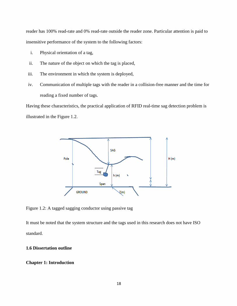
Having these characteristics, the practical application of RFID real-time sag detection problem is
illustrated in the Figure 1.2.
Figure 1.2: A tagged sagging conductor using passive tag
It must be noted that the system structure and the tags used in this research does not have ISO
standard.
1.6 Dissertation outline
Chapter 1: Introduction

19
This dissertation is organized and documented in five chapters. Chapter one introduces the general
background of the work and the rest of the dissertation is as follows:
Chapter 2: Literature Review
In this chapter, the general findings related to the topic and theories are summarized. The
arguments are made and therefore the gap to initiate the research on RFID is illustrated. Different
methods that are currently used by power utilities including power line carrier method which is
used by Eskom, state owned company (SOC) limited, South Africa to detect power line sag are
discussed. The literature is characterized and evaluated to find the real phenomenon behind the sag
and identify the impact on power system reliability and power quality. The syntheses of new
technologies which are at simulation stage in particular such as Global Positioning System (GPS)
are also viewed and drawbacks are given. Advantages of RFID sag detection method over the
current methods are addressed.
Chapter 3: System structure
The main aim of this chapter is to present the state of power transmission line sag detection and
how RFID contribute in real-time measurement of the sag (conductor vertical position). RFID-
Radar system is presented as an effective technology for power line sag detection in real-time. The
performance of passive ultra-high frequency (UHF) RFID system in practice is given and the
strength of radar system for long range measurement is analyzed. Our radar system is evaluated
under different weather conditions, with its read rate, electromagnetic interference and corona
effect on the tag performance.
Chapter 4: Analysis and Results

20
The data obtained from the radar system is presented in this chapter. The result of sag detection is
analyzed to show the performance of the proposed monitoring system.
Chapter 5: Conclusion and Discussion
The findings are discussed and conclusion is made in this chapter. The tag sensitivity on metal
conductor object is better off seen from 8mm than that of a free space. Tag reflection from the
surface of a wooden object is not bigger in such that it requires greater power for tag that is close to
the surface. The graphical representation of result shows that active tags which are battery assisted
have shown to give more precision and better range than passive tags.
CHAPTER 2 LITERATURE REVIEW
2.1 Introduction of this chapter
In this chapter the phenomenon of sagging and galloping is discussed in details and explanations
are given based on previous theories and practical historical events. Power quality problem due to
conductor sag is also detailed. Current methods used to measure conductor sag are presented and
the radio frequency identification theory and its advantages in transmission line sag detection are
addressed.
2.2 Transmission line sagging
Overhead transmission lines for transport of high-voltage electricity are cables made of aluminum
alloy, suspended between high towers in the countryside. One cable of several kilometers between
two anchoring towers and carried by several towers in a row is called a section. The part of a
section that is suspended between two towers is called a span. As the cable is connected to the

21
towers by a freely movable suspension string or isolator, the dynamical motion of neighboring
spans are coupled. In wintertime when the cable is covered by snow or ice, the cables are
vulnerable to large scale vertical vibration in combination with a torsional vibration sustained by
steady cross winds. This aero-elastic instability is known as galloping. For high enough amplitudes
neighboring conductors may get close enough for the air-insulation to break down, causing a short-
circuit and structural damage to the cables. It is known from observations that even a small wind
force is sufficient to maintain a galloping vibration (Rienstra S.W., 1988 pp. 133-134).
The transmission line might have length extension of a line conductor caused by many factors such
as overheating due to excessive current loading, wind vibration; ice force and etcetera. The length
extension results in the increase of sagging.
2.2.1 Power quality disturbances
It is important to define the performance of a power system and discuss the power quality
incidences on utility system for customer satisfaction and economic impact.
As discussed in the first chapter, conductor sag might result into voltage sag and possibly a power
disturbance. This can also be seen as an interruption which is defined as a 0.9pu reduction in
voltage magnitude for a period less than one minute. An interruption is characterized by the
duration as the magnitude while transient is an increase of RMS voltage for longer than one
minute. Typically the voltage magnitude is 1 to 1.2V per -unit which is caused by switching off the
large load from the system, energizing a capacitor bank, poor tap settings on the transformer or
inadequate voltage regulation (Amin, S.M and Wollenberg, B.F., 2002). Overvoltage’s can be
caused by equipment damage and failure. Harmonic issues are caused by the increasing power
electronic devices like variable speed drives and inverters, which increases the harmonic distortion

22
in the power system. The presence of harmonics in the system could also cause several unwanted
effects in the system including excessive transformer heating or overloading and failure of power
factor correcting capacitors, therefore it is related to transmission line sagging. The maximum total
harmonic distortion which is acceptable on the utility system is 5% at 2.3 to 69kV, 2.5% at 69 to
138kV and 1.5% at higher than 138kV voltage levels (IEEE Std. 1250, 1995).
Voltage imbalance is normally caused by unequal distribution of loads amongst the three phases.
At three phase distribution level, unsymmetrical loads at industrial units and un-transposed lines
can result in voltage imbalance. Voltage imbalance is of extreme importance for three phase
equipment such as transformers, motors and rectifiers, for which it results in overheating due to a
high negative sequence current flowing into the equipment. The asymmetry can also have an
adverse effect on the performance of converters, as it results in the production of harmonics.
2.2.2 Determination of sag
The energized conductors of transmission and distribution lines must be constructed in such a way
that the possibility of their potential to touch ground is regularly tracked. Overhead conductors,
however elongate with time, temperature and tension, thereby changing their original positions
after installation. Despite the effects of weather and loading on a line, the conductors must remain
at safe distances from buildings, objects, and people or vehicles passing beneath the line at all
times. To ensure this safety, the shape of the terrain along the right of way, the height and lateral
position of the conductor support point, and the position of the conductor between support points
under all wind, ice, and temperature conditions must be known (Douglass D.A and Trash R., 2013
pp14-2). The shape of the catenary changes with conductor temperature, ice and wind loading, and
time. To ensure adequate vertical and horizontal clearance under all weather and electrical
loadings, and to ensure that the breaking strength of the conductor is not exceed, the behavior of

23
the conductor catenary towards the consumer, under all conditions must be known before the line is
designed. The future behavior of the conductor towards the external forces is determined through
calculations commonly referred to as sag-tension calculations.
Sag tension calculations predict the behavior of conductor based on recommended tension limits
under varying loading conditions. These tension limits specify certain percentages of the
conductors rated breaking strength that is not to be exceeded upon installation or during the life of
the line. These conditions, along with the elastic and permanent elongation properties of the
conductor, provide the basis for determining the amount of resulting sag during installation and
long-term operation of the line. Accurately determined initial sag limits are essential in the line
design process, to enable dynamic rating of the networks. According to (SANS10280/NRS 041-
1:2008), conductors current ratings can be determined by either assuming the worst case cooling
conditions using deterministic method or by assessing the risk of an unsafe condition arising that is
probabilistic method. For deterministic ratings the weather assumptions is in accordance with guide
of weather parameter selection for overhead conductor rating given by (Cigre, brochure 299).
These include the following:
Table 1: Weather parameter selection
Weather assumption Parameter value
Wind speed perpendicular to line 0.6𝑚/𝑠
Absorptivity and emissivity 0.8
Solar radiation 1000𝑤/𝑚2
Ambient temperature 40℃
Although this parameters are followed from the initial design stage of transmission networks,
extreme weather conditions have been experience dramatically recently in South Africa and the

24
factors are unknown. This could escalate the sag and eventually the poor power system
performance and instability.
Final sags and tensions depend on initial installed sags and tensions and on proper handling during
installation. The final sag shape of conductors is used to select support point heights and span
lengths so that the minimum clearances will be maintained over the life of the line. If the conductor
is damaged or the initial sags are incorrect, the line clearance may be violated or the conductor may
break during heavy ice or wind loading (Douglass D.A. and Trash R., 2013 pp14-2).
2.2.3 Level Spans
The shape of a catenary is a function of the conductor weight per unit length, 𝑤, the horizontal
component of tension, 𝐻, span length, 𝑆, and the maximum sag of the conductor 𝐷. Conductor sag
and span length are illustrated in Figure 2.1 for a level span. The exact catenary equation uses
hyperbolic functions. Relative to the low point of the catenary curve shown in Figure 2.1, the
height of the conductor, 𝑦(𝑥), above this low point is given by the following equation (Ramon R.,
1987 pp. 851-856):
𝑦(𝑥) = 𝐻
𝑤cosh ((
𝑤
𝐻𝑥) − 1) =
𝑤(𝑥2)
2𝐻 (2.1)
For a level span, the low point is in the center, and the sag, D, is found by
𝐷 = 𝐻
𝑤(cosh (
𝑤𝑠
2𝐻) − 1) =
𝑤( 𝑆2)
8𝐻 (2.2)

25
At the end of the level span, the conductor tension, T, is equal to the horizontal component plus the
conductor weight per unit length, 𝑤, multiplied by the sag, 𝐷 as shown in the equation below:
𝑇 = 𝐻 + 𝑤𝐷 (2.3)
Figure. 2.1 The catenary curve for level spans (Rienstra S.W., 1988 pp. 133-134)
2.2.4 Conductor length
Conductor length from the low point of the catenary from either direction of the sag can be
obtained as follows:

26
𝐿(𝑥) = (𝐻
𝑤𝑆𝐼𝑁𝐻(
𝑆𝑤
2𝐻)) = 𝑆 (1 +
𝑥2(𝑤)2
6𝐻2) (2.4)
For a level span, the conductor length corresponding to 𝑥 =𝑆
2 be the half of the total conductor
length and the total length 𝐿, is:
𝐿 = (2𝐻
𝑤) 𝑆𝐼𝑁𝐻 (
𝑆𝑤
2𝐻) = 𝑆 (1 +
𝑥2(𝑤2)
24𝐻2) (2.5)
The parabolic equation for conductor length can also be expressed as a function of sag, 𝐷, by
substitution of the sag parabolic equation, giving:
𝐿 = 𝑆 + 8𝐷2
3𝑆 (2.6)
A conductor should have a slack to avoid high stress level. This Slack is the difference between the
conductor length, 𝐿, and the span length 𝑆. The parabolic equations for slack may be found by
combining the preceding parabolic equations for conductor length 𝐿, and sag 𝐷 (Rienstra S.W.,
1988 pp. 133-134).
𝐿 − 𝑆 = 𝑆3 (𝑤2
24𝐻2) = 𝐷2 (
8
3𝑆) (2.7)
The slack of the conductor in a span can contribute to the changes in conductor sag.
Such that sag 𝐷 𝑖𝑠:
𝐷 = √3𝑆(𝐿−𝑆)
8 (2.8)

27
For inclined spans: they may be analyzed using essentially the same equations that are used for
level spans. The catenary equation for the conductor height above the low point in the span is the
same. However the span is considered to be consisting of two separate sections, on to the right of
the low point and the other to the left of the low point. The shape of the catenary relative to the low
point is unaffected by the difference in suspension point of elevation. In each direction from the
low point, the conductor elevation, relative to the low point is given by:
𝑦(𝑥) =𝐻
𝑤𝑐𝑜𝑠ℎ ((
𝑤
𝐻𝑥) − 1) =
𝑤𝑥2
2𝐻 (2.9)
Figure 2.2: shows the inclined catenary (Rienstra S.W., 1988 pp. 133-134)

28
The horizontal distance 𝑋𝐿 from the left support point to the low point in the catenary is
𝑋𝐿 = 𝑆
2(1 +
ℎ
4𝐷) (2.10)
The horizontal distance, 𝑋𝑅 from the right support point to the low point of the catenary is:
𝑋𝑟 = 𝑆
2(1 −
ℎ
4𝐷) (2.11)
From the inclined catenary span 𝑆1 is the straight-line distance between support points, 𝑆,
horizontal distance between supports, ℎ, vertical distance between support points, 𝐷, the sag
measured vertically from a line through the points of conductor support to a line tangent to the
conductor.
The midpoint sag 𝐷 is approximately equal to the sag in a horizontal span equal to the length to the
inclined span, knowing the horizontal distance from the low point to the support in each direction,
the preceding equations for 𝑦(𝑥), 𝐿, 𝐷 𝑎𝑛𝑑 𝑇 can be applied to each side of the inclined span, S1.
Knowing the horizontal distance from the low point to the support point in each direction, the
preceding equations for 𝑦(𝑥), 𝐿, 𝐷, 𝑎𝑛𝑑 𝑇 can be applied to each side of the inclined span. The total
length in the inclined span is equal to the sum of the lengths in 𝑋𝑅 and 𝑋𝐿 sub-span sections
(Ramon G., 1987 pp. 851-856).
𝐿 = 𝑆 + (𝑋𝑅3 + 𝑋𝐿
3) (𝑤2
6𝐻2) (2.12)
In each sub-span, the sap is relative to the corresponding support point elevation
𝐷𝑅 = 𝑤𝑥𝑅2 ∗
1
2𝐻 (2.13)
𝐷𝐿 = 𝑤𝑥𝐿2 ∗
1
2𝐻 (2.14)

29
Where 𝐷𝑅 and 𝐷𝐿 is the sag on the right and on the left.
One of the important factors in designing the transmission network is considering the ice and wind
conductor loads. During incidents of heavy ice or wind loads, the conductor catenary tension
increases dramatically along with the loads on the angle and dead-end structures. Both the
conductor and its supports can fail unless high-tension conditions are considered in the line design.
The loads must be accounted for in the line design process so they do not have a detrimental effect
on the line. Ice in the overhead conductor may take several forms such as rime ice, wet snow and
glaze ice. The impact of low density ice formation is usually considered in the design of line
sections at high altitudes. The formation of ice on the overhead conductors has the following
influence on line design; that is the maximum vertical conductor loads that structures and
foundations must withstand, in combination with simultaneous wind loads; ice loads also determine
the maximum transvers loads on structures (Alexis Polycarpou, 2011).
The sag permanent increase in due time in regions of heavy ice loads may be due to ice loadings.
Ice loads for use in designing lines are normally derived on the basis of past climate experience and
weather conditions, national energy regulations code of practice and the historical weather data.
Mean recurrence intervals for heavy ice loadings should be the function of local conditions along
various routings. Hence considering the dynamic climate changes in the initial stage is vital. The
current transmission networks are not guaranteed for climate changes in Africa.
2.2.5 Wind loadings on overhead lines
They influence line design in a number of ways: that is the maximum span between structures may
be determined by the need for horizontal clearance to the edge of right of way during moderate
winds, the maximum transverse loads for tangent and small angle suspension structures are often
determined by infrequent high wind speed loadings and permanent increases in conductor sag may

30
be determined by wind loading in areas of light ice (Olsen R.G. and Edwards K.S., 2002 pp.1142-
1152).
2.2.6 Maximum Conductor Tension
It is the tension of the conductor allowable to conductor’s rated breaking strength. Transmission
lines under wind or ice loading experience high level tension which result into Aeolian vibration
and unsafe levels. Under everyday conditions, tension limits should be specified to control the
vibration. Aeolian vibration levels, and thus appropriate unloaded tension limits, vary with the type
of conductor, the terrain, span length, and the use of dampers. Special conductors such as ACSS
SDC and VR bring about high self-damping properties and may be installed to the full limits. The
conductor length depends on span and sag and is not directly dependent on conductor tension,
weight or temperature (Dale Douglass, Paul Springer, IEEE Technical brochure, 2013).
2.2.7 Thermal Elongation
Increase in temperature causes an increase in length and sag and decreases the tension. Concentric-
lay stranded conductors, particularly non-homogenous conductors such as ACSR, are not
inextensible. Rather, they exhibit quite complex elastic behavior. Initial loading of conductors
results in elongation behavior substantially different from that caused by loading many years later.
Also high tension levels caused by heavy ice and wind loads cause a permanent increase in
conductor length, affecting subsequent elongation under various conditions. ACSR and AAC
conductors elongates with increasing conductor temperature (DA Douglass and Ridley Trash 2013
pp.14-2).
(Muhr et al 2005 pp.14) presents the results of a study of elongation mechanism of an overhead
conductor, which shows that the deflection of the tension insulators affects the sag behavior of the

31
close-by spans. In the rod distribution of a flat overhead line symmetric, the deflection of the
suspension insulators was negligible and had no significant effect on the sag calculation. The
deflection of the suspension insulators is not negligible when the rod distribution is asymmetric.
The span with the largest distance between the rods will sag much more than the smaller spans
(Olsen R.G. and Edwards K.S., 2002). The elongation of the overhead conductor reduces this
safety distance. The main point of the calculations is that the deflection of the suspension insulators
affects the sag and the phase to earth clearance significant by asymmetrical rod distribution. The
elongation of the overhead conductors caused by everyday stress leads to an increasing of the sag.
During the planning and construction lower sag than necessary gives a safety distance to the
regulation clearance. With sag verification of aged overhead lines by measurement or calculation,
the reliability of the overhead line can be improved. Depending on the system voltage and the
object type, the minimum phase to earth clearance can be assured (Thomas G., 2002).
The common practice is to assume that power line conductors are straight horizontal wires of
infinite length. In fact, they are periodic catenaries, the sag of which depends on individual
characteristics of the line and on environmental conditions. Consideration of catenaries effects in
the literature is scarce, since most often they are assumed to be negligible. Whenever analysis of
the power line is concentrated on phenomena in close proximity to the conductors, the straight wire
approximation must be critically reviewed (Ramon G., 1987).
2.2.8 The occurrence of galloping to sag
2.2.8.1 Types of motions
(Anjo K., et al 1974) indicate that conductor motions can be large enough to cause flashovers
between adjacent phases, especially when the phases are above each other. The vertical motion
may result from a combination of two or three loop modes. The swinging of the suspension points
32
longitudinally to the line, referred to above, are caused by the variation in tension that can
accompany galloping, and they act to couple the galloping motions in adjacent spans.
When the spans are on quasi fixed supports, such as in many lower voltage distribution lines, the
motions are commonly in the two-loop mode but with very high amplitudes (several times the sag
observed), in such severe cases tension changes, despite the two loops mode, can be quite high.
The amplitudes are again similar to each other in the different spans, due to feed-through at the
supports, which can occur because this class of line is frequently supported on wood poles with
cross arms, which allow some longitudinal support point movement (Admirat P., et al 1988). In
addition to causing flash over’s between phases, galloping can lead in to agitation of sag
phenomenon which could damage the structures due to twisting of the wood cross arms and poles
accompanying synchronous motions of the phases.
(Chadha J., 1974b) shows that the common designs of overhead transmission lines are short line
sections between dead-ends. Linear analysis of the motions calculation shows that for the modes at
0.386 and 0.403Hz, there is only small variation in tension during galloping. This is because when
one span is at its upwards extreme of motion, there is another span at the downward extreme. The
variations in the arc length of the two spans compensate each other by means of swinging of the
suspension support between them.
2.2.8.2 Factors influencing a transmission line galloping
i. Ice accretion type and shape (eccentricity, weight, and aerodynamic properties)
ii. Sagging Conditions (effect on vertical frequencies)
iii. Wind velocity (with limited effects of turbulence and orientation as detailed)

33
iv. Conductor self-damping (vertical, torsion) in the low frequency range (including span end-
effects)
v. Span lengths (including all spans of a section) and section length
vi. Longitudinal stiffness at attachment point on tension tower
vii. Yoke plate assembly (tension and suspension tower)
viii. Number of sub conductors and their arrangement
ix. Sub conductors spacing
x. Ration vertical frequency for each mod in the presence of wind
2.2.8.3 A view of Overhead line aerodynamics
When the shear center in the case of a conductor is viewed, the forces and moments acting at a
known location need to be considered. This requires the introduction of an aerodynamic pitching
moment about the new location. The evaluation of lift, drag and pitching moment is usually done in
a wind tunnel on a fixed, rigid cylinder on which the ice shape has been reproduced (Gartshore I.S.,
1973). The evaluation of such forces and moments on a fixed wind tunnel model rather than a
moving one is still a concern.
Figure 2.3: Aerodynamic characteristic of an iced conductor (Gartshore I.S., 1973)

34
The conductor, subject to a wind, U0, is shown at a time, t, during vertical torsional motion.
Aerodynamic forces, fL, and fD, and moment, MW, act at the shear Centre.
The conductor is assumed to move vertically upwards with a positive vertical speed. The initial ice
position is Θice and Θ is the actual rotation of the conductor φ is the angle of attack and is positive
anticlockwise. The drag force, fD, is oriented in the direction of the relative wind speed, vr (the
combination of U0 and the conductor's vertical speed). The lift force, fL, is perpendicular to the
drag force and positive upwards. The pitching moment is positive anticlockwise. We believe that
the analysis on the forces acting upon the conductor helps in the dynamic rating of future
transmission networks. It therefore important to carefully consider every cause of motion in the
conductor that leads to conductor sagging dangerous situation.
Looking at the stability conditions or (reduced amplitude), the conductor self-damping, ice
position and ice aerodynamic are very complex to estimate. This complicates the parameter line
predictions for voltage rating or temperature, stress and young’s modulus elasticity. Reference
(Gurung C.B., et al 2002) shows that the bundle moment of inertia plays a major role in the
instability criterion. The bundle conductor moment of inertia’s main contributors are the sub
conductor mass and bundle diameter, which is an important factor for galloping and sagging. Most
of the time, the diameter of the bundle is fixed by other considerations such as corona effect and
manufacturer standardization. However there are some exceptions. In theory an increased bundle
moment of inertia decreases the risk of instability. However the same cannot be said concerning
the amplitude, if instability criterion remains violated. An increase in sub conductor spacing
increases both the moment of inertia of the bundle and its torsional stiffness. In the absence of any
anti-galloping device however, these two increases unfortunately compensate each other so that
the effect on torsional frequency is insignificant (Halsan K.A., et al 1998).
35
2.2.8.3.1 Conductor Self-damping
The amplitudes of galloping that actually occur are determined by energy balance between the net
energy supplied through aerodynamic action, including effects of aerodynamic dampers and
mechanical dissipation in the galloping system. Mechanical dissipation mainly arises from self-
damping in conductors, hysteresis at span support, and damper (Harvard D.G., 1996). For
transverse vibration, self-damping is small but the highest Aeolian frequencies, and negligible at
galloping frequencies. Basically Elastic solid cannot dissipate more energy during a loading-
unloading cycle than is stored in it at the time of maximum loading (Harvard D.G., 1997). It is
common to refer to the loss coefficient of a solid, 𝜂 = 𝐷
2Π𝑈 Where D is the energy actually
dissipated in a full cycle and U is the maximum stored energy of strain (Hoerner S.F., 1965).
Dynamic loads resulting from galloping have been viewed as indicated by (Halsan K.A., et al
1998) the maximum dynamic loads are of the order of 1.2 times the static value at dead-ends and
1.7 times the static value at suspensions (Hillier R. and Cherry R.J., 1981). In areas subjected to
ice loads, suspension insulators everyday loads are normally very low compared to their tensile
strength; the ratio being of the order of one to nine. Consequently, the effect of galloping cyclic
loads is normally of no consequence. (Harvard D.G., 1978) indicates that on distribution lines
where pin type insulators are used, tie wire failures due to sagging happen occasionally. Where
clamp-top insulators are used, cement failure of the porcelain insulators due to the bending
moment applied on it during sagging has also been observed. Damage on insulators during the
sagging phenomenon is mostly occurring in the transmission lines when insulator string is being
clashed on the tower arm (Harvard D.G., 1984). However these damages are not related to a
fatigue phenomenon.
There are several methods and devices which are being used to detect the sag of a transmission

36
line which is discussed in section 2.3.
2.3 Different Methods used to measure conductor sag
2.3.1 Current transformers (CTs)
They are typically used for current measurement. However, they are expensive and limited by their
magnetic core characteristic and narrow bandwidth (Glorver B. and Bhatt H., 2003). The CTs
performance under distorted conditions is usually characterized by means of the frequency
response test. The method uses an excitation waveform (primary current) that consists of one
harmonic current, with adjustable amplitude and phase shift, superimposed on the fundamental
current. The measurement of harmonic current phasor is characterized by two basic errors (Glorver
B. and Bhatt H., 2003):
The h-order harmonic rations error:
%𝑒ℎ = 𝐾𝐼𝑠ℎ−𝐼𝑝ℎ
𝐼𝑝ℎ . 100 (2.15)
Where: 𝐾 = 𝑁𝑠/𝑁𝑝 is the nominal transformer ratio (Ns and Np are the secondary and primary
number of turns, correspondingly); 𝐼𝑠ℎ and 𝐼𝑝ℎ are the rms values of the secondary and primary
number of turns respectively); 𝐼𝑠ℎ and 𝐼𝑝ℎ are the rms values of the secondary and primary h-order
harmonic currents.
The h-order harmonic phase angle error:
𝜀ℎ = 𝛼𝑠ℎ− 𝛼𝑝ℎ (2.16)

37
Where: 𝛼𝑠ℎ and 𝛼𝑝ℎ are the secondary and primary harmonic current phase angles in degrees,
respectively. These indexes were used to characterize two current transformers excited by a non-
sinusoidal current (Glorver B. and Bhatt H., 2003). Basically Current transformers measures the
flow of current in a conductor not the position of the conductor, therefore cannot detect sag. There
are some existing devices that can directly or indirectly measure sag of transmission lines.
2.3.2 Power Line Carrier Method (PLC)
It determines average overhead conductor height variations by correlating sag with measured
variations in the amplitude of signals propagating between PLC stations (Mensah C., 2011). The
PLC-SAG technique is fundamentally based on the theory of natural modes supported by multi-
conductor transmission lines. PLC system Provide a highly reliable infrastructure for the
transmission and reception of data, speech and protection signals between stations.
2.3.2.1 PLC Attenuation Sensitivity and Height Variation
Attenuation of the PLC signal is due to two major contributions: that is attenuation due to the
transmission line, including the effect of ground resistivity; which is complex and requires the
rigorous theoretical analysis of modal propagation on multi-conductor transmission lines and
attenuation due to the coupling system, is simple to compute.
With outer-to-outer phase coupling, the signal level is sensitive to variations in line height. The
PLC-SAG technique makes use of this phenomenon to remotely monitor the average height
movement of the OHTL (Cataliotti et al., 2008).
2.3.2.2 PLC based on the Modal theory

38
The voltage propagation is referred at the product of impedance and admittance matrices given by
𝑃 = 𝑍𝑌 (2.17)
The voltage propagation matrix is determined in terms of its eigenvalue matrix λ and eigenvectors
𝐸𝑣 such that
𝑃 = 𝐸𝑣 𝐸𝑣−1 𝜆 (2.18)
The eigenvectors are determined by the fixed, physical geometry of the transmission line. The
eigenvalues describe the variable or dynamic characteristics of the solution. The modal of the
system is constructed from the eigenvector columns, and is fixed by the transmission lines physical
geometry. For a horizontal transmission line, the columns of the Clarke matrix give a good
approximation of the natural modes (Wernich V. and Arthur B., 2008).
[
1
21 1
−1 0 11
2−1 1
] = 𝑀 (2.19)
Mode 1 is defined by the first column and is the mode with the lowest attenuation. Mode 2, the
differential mode, is defined by column 2 and it propagates with a lower phase velocity and higher
attenuation than mode 1. It makes a significant contribution to the total received signal. Mode 3 is
the common mode and is heavily attenuated due to ground losses and can be neglected. Relative
amplitudes of the modes, which are excited on transmission line, are determined by the voltage
excitation vector applied to the line by PLC coupling configuration.
2
ym mg
t
(2.20)
39
Eigenvalues of the propagation Matrix describe the dynamic characteristics of the different natural
modes of the system. Thus the attenuation and phase retardation of modes are associated with the
eigenvalues (Wernich V. and Arthur B., 2008).
The horizontal transmission line can be determined in terms of the voltage on phase 𝑁𝑉𝑝𝑁 as given
by the following matrix;
[𝑒−𝛾1𝑥 0 00 𝑒−𝛾2𝑥 00 0 𝑒−𝛾3𝑥
] 𝐸𝑣 𝐸𝑉−1 [
𝑉𝑝1𝑉𝑝2𝑉𝑝3
] = 𝑉𝑥 (2.21)
Where 𝑒−𝛾3𝑥 is the scalar factor, 𝐸𝑣 is the sending end voltage
This is not accurate as conductors swing differently in different conditions more specifically when
we consider the wind induced vibrations. Although this method is currently used by ESKOM South
Africa, it is clear that advancements are needed in order to obtain measurements in real time. This
method can only obtain the sag through average calculation of signal amplitudes.
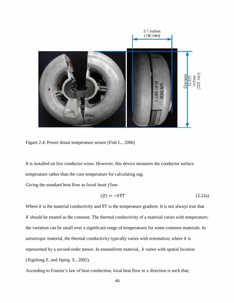
2.3.3 Power donut
It is an instrument platform for remote monitoring of overhead transmission lines, powered directly
from the conductor electric field (Xignlong Z. and Jiping S., 2002). This instrument performs
measurements of voltage, current, conductor temperature and the angle of inclination.
40
Figure 2.4: Power donut temperature sensor (Fish L., 2006)
It is installed on live conductor wires. However, this device measures the conductor surface
temperature rather than the core temperature for calculating sag.
Giving the standard heat flow as 𝑙𝑜𝑐𝑎𝑙 ℎ𝑒𝑎𝑡 𝑓𝑙𝑜𝑤.
(𝑄) = −𝑘∇𝑇 (2.22a)
Where 𝑘 is the material conductivity and ∇𝑇 is the temperature gradient. It is not always true that
𝐾 should be treated as the constant. The thermal conductivity of a material varies with temperature;
the variation can be small over a significant range of temperatures for some common materials. In
anisotropic material, the thermal conductivity typically varies with orientation; where 𝑘 is
represented by a second-order tensor. In nonuniform material, 𝑘 varies with spatial location
(Xignlong Z. and Jiping S., 2002).
According to Fourier’s law of heat conduction, local heat flow in 𝑥 direction is such that;

41
𝑞𝑥 = −𝑘𝑑𝑇
𝑑𝑥 (2.22b)
Where k is the thermal conductivity (W/m ͦ C). Q is the vector quantity and can have x, y and z
components. Therefore the heat transfer in a power transmission line conductor cannot determine
the vertical movement of the conductor in real time. However it can help in the dynamic design of
the line rating at initial stage.
In addition, this platform is very expensive and its installation requires working with live wires is
more risky.
2.3.4 Global Positioning System
Application of the global positioning system (GPS), based on a constellation of 24 satellites, which
uses the Navigation satellite Timing and Ranging (NAVSTAR) developed, launched, and
maintained by the United States government (Thomas G., 2002).
It is a worldwide navigation and positioning resource for both military (i.e., precise positioning
service) and civilian (i.e., standard positioning service) applications. This method relies on accurate
time-pulsed radio signals in the order of nanoseconds from high altitude Earth orbiting satellites of
about 11 000 nautical miles, with the satellites acting as precise reference points. These signals are
transmitted on two carrier frequencies known as the L1 and L2 frequencies. The L1 carrier is
1.5754GHz and carries a pseudo-random code (PRC) and the status message of the satellites. There
exist two pseudorandom codes: the coarse acquisition (C/A) and the precise (P) codes. The L2
carrier is 1.2276GHz and is used for the more precise military PRC. The signals from four or more
satellites are received by a specially designed GPS receiver, and the following simultaneous
equations are solved (Thomas G., 2002):
42
(𝑋𝑠𝑘 − 𝑋𝑟𝑗 )2 + (𝑌𝑠𝑘 − 𝑌𝑟𝑗)2 + (𝑍𝑠𝑘 − 𝑍𝑟𝑗)
2 = (𝑅𝑘 − 𝑑𝑇) (2. 23)
𝐾 = 1, 2… N 𝑘 = 1,2, … . , 𝑛 𝑛 ≥ 4 (2.24)
Where (𝑋𝑠𝑘,𝑌𝑠𝑘 , 𝑎𝑛𝑑 𝑍𝑠𝑘 ) represents the 𝑘𝑡ℎ satellite position (𝑋𝑟𝑗 𝑌𝑟𝑗, 𝑍𝑟𝑗) denotes the unknown
𝑗𝑡ℎ receiver position 𝑅𝑘denotes the range to 𝑘𝑡ℎ satellite, and 𝑑𝑇 is the unknown receiver clock
bias converted to distance. This gives the longitude and latitude of the receiver (i.e., defectively x
and y), the altitude of the receiver (effectively z), and the time that the measurement was made t.
interestingly, the GPS transmission is made at low power level (the signal strength at the point of
reception is about -90 to -120dBm). At this power level, the SNR is very low at the surface of the
Earth. The attenuation of the noise is accomplished by averaging the received signal. The noise is
averaged and a distinctively coded signal appears as an output. The averaging processes, as well as
the solution of (1) are the main time limiting processes that determine how often a GPS
measurement can be made (Fish L., 2006).
There is a potential in this technology, although there are some errors contributing to estimates.
The differential GPS is generally used in order to decrease the selective availability errors. This
mode consists of the base and the rover. The main disadvantage of the DGPS is the requirements of
a second GPS receiver and corresponding communication equipment between the base and rover
instruments. It is costly, and its performance in a HV environment is unreliable.
The accuracy of the direct instrumentation of overhead power line conductor sag measurement is
about 19.6 cm range and 70% of the time. In the implementation of this technology, the
phenomenon of the corona discharge in a transmission line conductor is a challenge in that it
creates potentially intolerable conditions for radio reception in the 930MHz and 1.5 GHz frequency
bands (Edelsein A., 2007).

43
This method relies on accurate time-pulsed radio signals in the order of nanoseconds from high
altitude Earth orbiting satellites of about 11 000 nautical miles, with the satellites acting as precise
reference points. This technique is promising; however the challenge such as electromagnetic
interference (EMI) from the phase conductors is questionable.
2.3.5 Image processing based on camera
It is a costly technique and its installation requires contact with phase conductors for placing the
targets. In image processing an edge is the boundary between an object and its background
appearance. This represents the frontier for single objects. If the edges of image objects are
identified with precision all objects can be located and their properties such as area, perimeter and
shape can be calculated. Edge detection is an essential tool for image processing technology.
There are two advanced and optimized edge detector in image processing, namely canny edge
detectors and infinite symmetric exponential filter (Martin A and Tosunoglu S., 2002). These
detectors follow different algorithms such that for canny edge detection, it is represented as
follows:
Read the image I.
Convolve a 1D Gaussian mask with I.
Create a 1Dmask for the first derivative of the Gaussian in the x and y directions.
Convolve I with G along the rows to obtain Ix, and down the columns to obtain Iy.
Convolve Ix with Gx to have Ix’, and Iy with Gy to have Iy’.
Find the magnitude of the result at each pixel
' 2 ' 2( , ) ( , ) ( , )x yM x y I x y I x y (2. 25)
Infinite Symmetric Exponential Filter uses another optimization function to find the edge in an

44
image this function can be written as:
2 '2
2 0 0
4
4 ( ) . ( )
(0)N
f x dx f x dx
Cf
(2.26)
The function 𝐶𝑁 is minimizing with an optimal smoothing filter for an edge detector, which result
into an infinite symmetric exponential filter, as follows;
( ) , ( , ) .
2
p x yp xpf x e f x y a e
(2.27)
The filter in the infinite symmetric exponential filter edge detector is presented as one dimensional
recursive filter. By presuming the 2D-filter function real and continuous, it is given by;
1
,1
x yb b
f i jb
(2.28)
In some instances, image processing technique, uses automatic image analysis technique for
extracting information from the line insulators. This concerns the detection of snow overage on
insulators on the line and the detection of swing angles of insulators with respect to the vertical
position. It must be clear that no real-time detection of the actual transmission line is made by this
technique; hence it cannot be translated or linked to real time dynamic rating of the line.
2.3.6 Electro-magnetic Coupling Method
45
Electromagnetic Coupling Method is based on the magnetic field surrounding the conductor (Olsen
R.G. and Edward K.S., 2002). For different line configurations, the grounded wire position and the
sag calculation need to be modified. Also, Electro Magnetic Interference from nearby transmission
lines cannot be neglected.
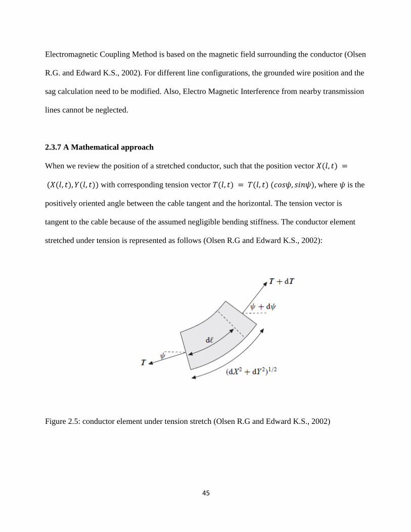
2.3.7 A Mathematical approach
When we review the position of a stretched conductor, such that the position vector 𝑋(𝑙, 𝑡) =
(𝑋(𝑙, 𝑡), 𝑌(𝑙, 𝑡)) with corresponding tension vector 𝑇(𝑙, 𝑡) = 𝑇(𝑙, 𝑡) (𝑐𝑜𝑠𝜓, 𝑠𝑖𝑛𝜓), where 𝜓 is the
positively oriented angle between the cable tangent and the horizontal. The tension vector is
tangent to the cable because of the assumed negligible bending stiffness. The conductor element
stretched under tension is represented as follows (Olsen R.G and Edward K.S., 2002):
Figure 2.5: conductor element under tension stretch (Olsen R.G and Edward K.S., 2002)
46
Now considering a small cable element, 𝑑𝑙. Due to gravity, cable tension, and inertial forces, this
element is stretched however the mass remain the same. A conductor element is elongated in
proportion to tension, according to Hooke’s law, such that:
1
2 2 2 1 .T
dX dY dlEA
(2.29)
According to a Newton’s law, the internal tension and the external gravity forces are in equilibrium
with the inertial forces, such that;
𝑑𝑇 = (𝑔𝑒𝑦 + 𝑑2𝑦
𝑑𝑥2)𝑚 𝑑𝑙 (2.30)
1 cos , 1 sin ,X T Y T
l EA l EA
(2.31)
The equation result in the limit 𝑑𝑙𝑦𝑖𝑒𝑙𝑑𝑠→ 0 are given by
2
2,
1
T X Xm
Tl l t
EA
(2.32)
2
2,
1
T Y Ym mg
Tl l t
EA
(2.33)
47
2 2 2
1 .X Y T
l l EA
(2.34)
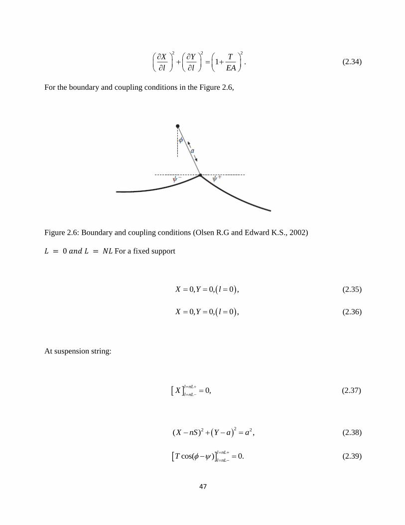
For the boundary and coupling conditions in the Figure 2.6,
Figure 2.6: Boundary and coupling conditions (Olsen R.G and Edward K.S., 2002)
𝐿 = 0 𝑎𝑛𝑑 𝐿 = 𝑁𝐿 For a fixed support
0, 0, 0 ,X Y l (2.35)
0, 0, 0 ,X Y l (2.36)
At suspension string:
0,l nL
l nLX
(2.37)
22 2( ) ,X nS Y a a (2.38)
cos( ) 0.l nL
l nLT
(2.39)

48
Where ϕ is the angle of the supension string
The mathematical approach help us to understand the problem of sag more and the behavior of the
transmission line under galloping conditions. Hence it only help us to reduce various problem
parameters in to a single clear problem phenomenon.
2.3.8 Magneto Resistive Sensors
Magneto resistive (MR) sensors were recently applied for sag measurement. It calculates the
current flow and line positions from the magnetic field emanated from the phase conductors
(Eldelstein A., 2007). Provided the sensitivity of the magnetic sensors is sufficient, the electric and
spatial information of the overhead line can be found by inverse calculation from the magnetic field
measured at the ground level. However the accuracy of this technique is questionable. Factors such
as multiple power conductors, bundle conductors and image current due to a conducting ground
have to be taken in to consideration.
2.3.9 Autonomous Robot Technique
Autonomous robot technique based on simulations uses energy from the line and run along the
conductor while making the inspection. The energy absorbed by the robot comes from the line,
producing an increment in the line impedance and therefore, a voltage drop in the point of the line
where the robot is located during the inspection (Graham H., 2008). The stability and reliability of
this technique is questionable as the magnetic field emanated from the conductors always vary and
the storage of such. This system also requires more number of turns in the secondary side of the
current transformer to increase the power transmission to the system, therefore need the large ration
transformers. This is an expensive method.
49
2.4 Background of RFID
RFID technology has been around since World War II (1948), where it was used to help solders to
identify fighter plane. Although it was a crude vision and tags were very big in size. This
technology uses radio waves to automatically identify objects and alternatively provides a means
of storing data and retrieving data, through electromagnetic waves transmission to RF compatible
integrated circuit. The major applications of RFID extended to various industries in recent years;
including farm produce tracing, vehicle identification, entrance guards, and trade control (Bouc M.
et al., 2010). RFID may be seen as the next logical step in the progression of tracking system and
sensor networks because of technological advances in several fields. As we introduced this
technology in chapter one of the dissertation, we continue to detail the explanation of key
operational parameters that affect RFID performance in terms of range and throughput. We then
look at the scalability and security later.
2.4.1 The key parameters of RFID
The key parameters that affect range and data rate are interdependent as shown in the depend
encygraph of Figure 6. In this figure, the parameters and decision choices that the designers/users
of RFID system have control over are shown within the hexagons (Bouc M. et al., 2010).These
parameters include operating frequency, transmit power, bandwidth, digital modulation encoding,
and maximum tolerable bit error rate (BER).The key operational parameters that are affected by
those design parameters include operating distance (range) and system throughput (proportional to
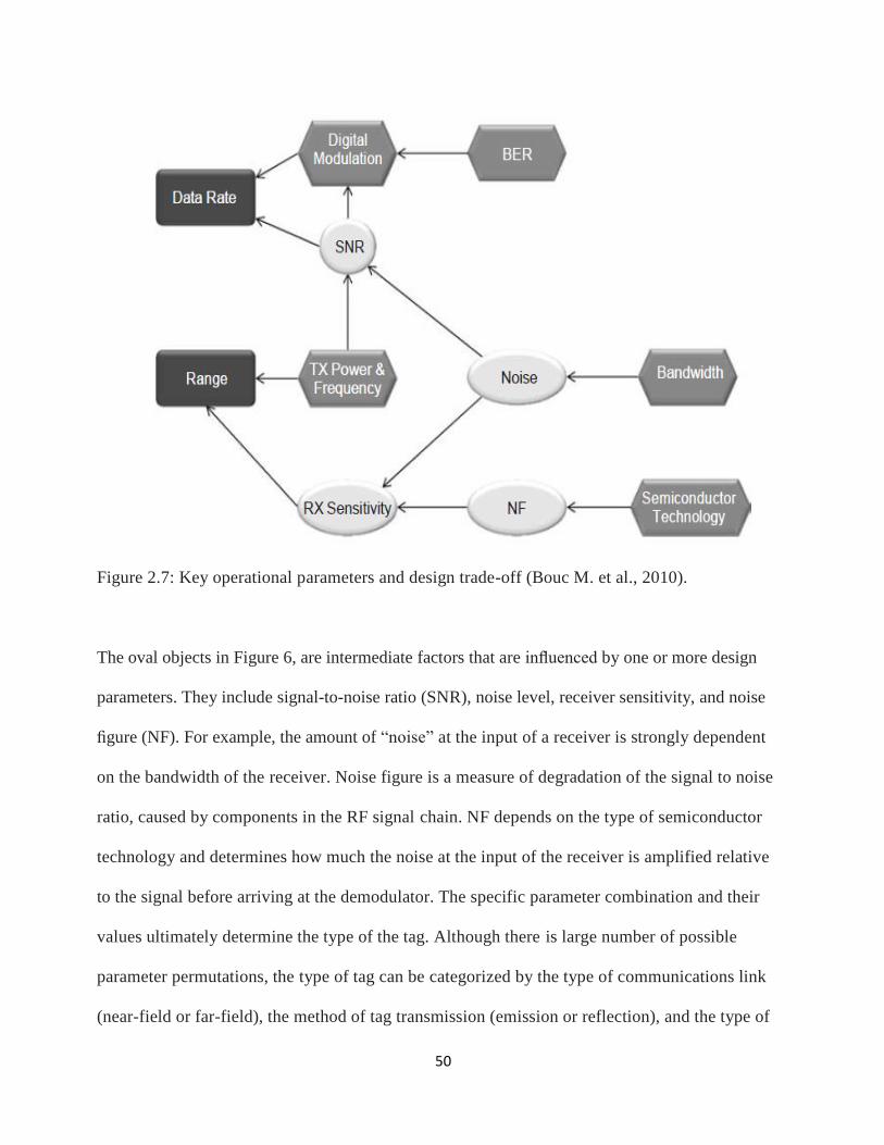
data-rate). These operational parameters are shown within the rectangles of Figure 2.7.
50
Figure 2.7: Key operational parameters and design trade-off (Bouc M. et al., 2010).
The oval objects in Figure 6, are intermediate factors that are influenced by one or more design
parameters. They include signal-to-noise ratio (SNR), noise level, receiver sensitivity, and noise
figure (NF). For example, the amount of “noise” at the input of a receiver is strongly dependent
on the bandwidth of the receiver. Noise figure is a measure of degradation of the signal to noise
ratio, caused by components in the RF signal chain. NF depends on the type of semiconductor
technology and determines how much the noise at the input of the receiver is amplified relative
to the signal before arriving at the demodulator. The specific parameter combination and their
values ultimately determine the type of the tag. Although there is large number of possible
parameter permutations, the type of tag can be categorized by the type of communications link
(near-field or far-field), the method of tag transmission (emission or reflection), and the type of
51
power supply (battery or energy harvesting). The far-field begins where the wave impedance
quickly settles towards the free-space impedance value of 377 ohms (Marrocco G., 2008).
For electrically small antennas, this distance is given by
𝑅𝑁𝐹 = 𝜆
2𝜋. (2.40)
The distance is essentially the radius of the near-field region around an antenna, and is less than
one foot for popular commercial UHF RFID system that operate in the 915MHz band. Passive tags
transmit data by reflecting power from the interrogator. This is also referred to as a backscatter
modulation for systems that operate in the far-field, and load modulation for systems that operate
in the near-field. Passive tags harvest energy from the interrogator instead of using a battery.
While an active UHF tags, make use of an on-board battery for the power needed to emit a
modulated RF signal that encodes the data (Marrocco G., 2008).
The most commonly utilized frequencies for both active and passive RFID operation are at or near
125 kHz, 13.65 MHz, 315 MHz, 433.92 MHz, 915 MHz, 2.45GHz, and 5.8GHz. Systems
operating in bands below 70MHz tend to operate in the near-field with inductively coupled coil
wire antennas because far-field antennas at those frequencies would be impractically large. The
majority of standards prescribe passive UHF RFID operation in the region between 860MHz and
960MHz because of its favorable output power and RF energy harvesting characteristics
(Bridgelall R., 1999).
Although passive tags are seen as cheaper because of not using the external power supply as
opposed to active tags, there are also constraints when it comes to sensitivity. (Bridgelall R., 1999)
shows that the lower the power a tag requires for activation and signal decoding, the greater its
52
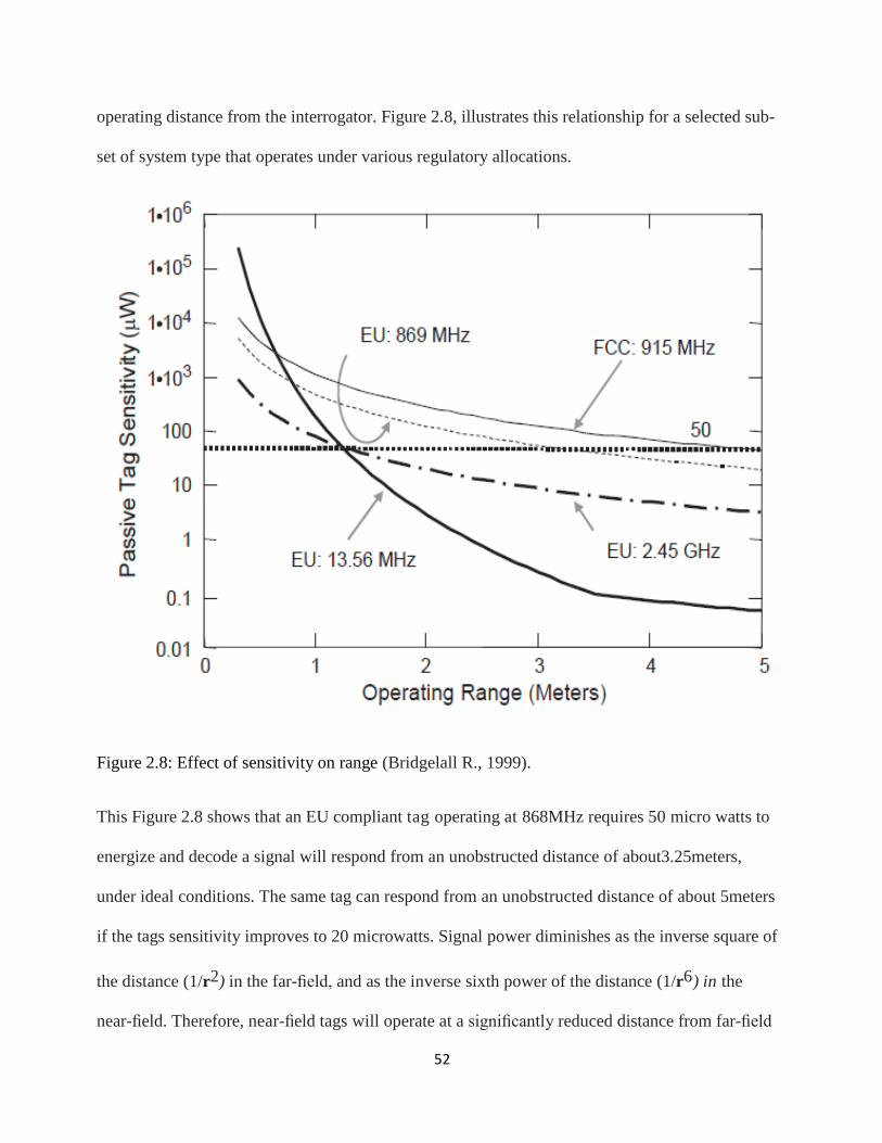
operating distance from the interrogator. Figure 2.8, illustrates this relationship for a selected sub-
set of system type that operates under various regulatory allocations.
Figure 2.8: Effect of sensitivity on range (Bridgelall R., 1999).
This Figure 2.8 shows that an EU compliant tag operating at 868MHz requires 50 micro watts to
energize and decode a signal will respond from an unobstructed distance of about3.25meters,
under ideal conditions. The same tag can respond from an unobstructed distance of about 5meters
if the tags sensitivity improves to 20 microwatts. Signal power diminishes as the inverse square of
the distance (1/r2) in the far-field, and as the inverse sixth power of the distance (1/r6) in the
near-field. Therefore, near-field tags will operate at a significantly reduced distance from far-field

53
tags of the same sensitivity.
Active tags have the advantage of longer range as opposed to passive and can continuously report
back to the reader without waiting for the energy from the reader. Passive tags receivers consist of
signal envelope detectors constructed from passive diodes or an equivalent construction. Such
detect a signal only when the input signal is sufficiently strong to overcome the passive diode
detector forward bias threshold (Mandal S. and Sarpeshkar R., 2007). Active tags utilize the on-
board battery to bias active rectification circuits, which substantially lowers this forward bias
threshold. The sensitivity difference can be significantly greater than 100dB. A lower UHF
operating frequency is preferred because of the more favorable energy capture characteristics of a
longer wavelength. The Fries far-field transmission formula for unobstructed narrowband
propagation gives;
2
_ .4
i tag sP P T rir
(2.41)
Such that the amount of signal power that the tag receives, Pi_tag proportional to the wavelength
λ squared. Ps is the power supplied by the interrogator, r is the operating distance, T is the
interrogator antenna gain, and ψri is the tag’s antenna sub-system gain when I is absorbing
energy.
2.4.2 Constraints on Interrogator Sensitivity for Passive UHF Tags
The interrogator signal received from a backscattering passive UHF tag decreases with free-
spaced is represented as follows (Mandal S. and Sarpeshkar R., 2007):
42.
4B sP P T ro
r
(2.42)
54
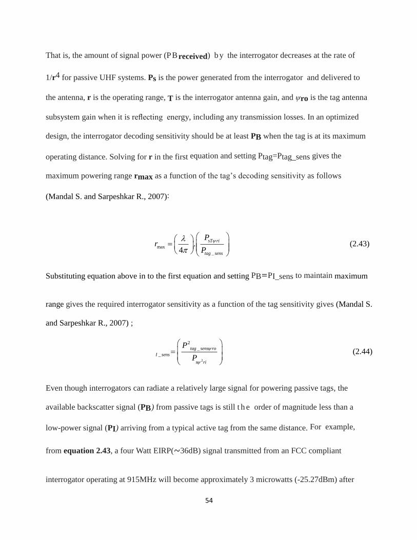
That is, the amount of signal power (PBreceived) b y the interrogator decreases at the rate of
1/r4 for passive UHF systems. Ps is the power generated from the interrogator and delivered to
the antenna, r is the operating range, T is the interrogator antenna gain, and ψro is the tag antenna
subsystem gain when it is reflecting energy, including any transmission losses. In an optimized
design, the interrogator decoding sensitivity should be at least PB when the tag is at its maximum
operating distance. Solving for r in the first equation and setting Ptag=Ptag_sens gives the
maximum powering range rmax as a function of the tag’s decoding sensitivity as follows
(Mandal S. and Sarpeshkar R., 2007):
max
_
.4
sT ri
tag sens
Pr
P
(2.43)
Substituting equation above in to the first equation and setting PB=PI_sens to maintain maximum
range gives the required interrogator sensitivity as a function of the tag sensitivity gives (Mandal S.
and Sarpeshkar R., 2007) ;
2
2
_
_
tag sens ro
I sens
s ri
P
P
(2.44)
Even though interrogators can radiate a relatively large signal for powering passive tags, the
available backscatter signal (PB) from passive tags is still t h e order of magnitude less than a
low-power signal (PI) arriving from a typical active tag from the same distance. For example,
from equation 2.43, a four Watt EIRP(∼36dB) signal transmitted from an FCC compliant
interrogator operating at 915MHz will become approximately 3 microwatts (-25.27dBm) after

55
travelling a distance of 30 meters in free space. A battery-powered backscatter tags will reflect a
portion of the tree microwatts towards the interrogator. In comparison, a low power active tag in
the same band will typically transmit 1 mill watt (0dBm) of signal, which is over 300 times more
powerful than the signal backscattered from a passive tag (Smith A.A., 1998). This means that an
interrogator with the same sensitivity can also decode the active tag’s response at a lower distance.
With all other parameters unchanged, increasing range means either increasing the average signal
power transmitted or increasing the receiver sensitivity. However, regulatory rules limit the
transmitted power, and the receiver noise figure bounds its sensitivity. The theoretical noise floor
is a function of bandwidth and temperature (Smith A.A., 1998).
It is clear that the power consumption of the passive tag is very important to consider when
designing the tag, this should go with the size of the tag as well. Advancement in polymer
electronic for fabrication of the tag is required.
For practical implementations, transmission power, noise figure, and bandwidth affect key
application level considerations such as power consumption, cost, and size. Increasing
antenna gain in order to increase the receive signal strength tends to increase the size of the
antenna. Higher antenna gain also favors transmission or reception in one direction over
others. Whistle lower gain antennas must be used if the application requires Omni-
directional performance. A lower noise figure amplifier increases sensitivity but also tends
to demand more power or require a more expensive semi-conductor technology (Gray P.R.
et al 2001).
If we need more output power from the interrogator, it means we need to put additional heat
sinks, and increase their size because interrogator’s power consumption will increase.
Therefore when designing RFID system factors such as bandwidth, size, range, power
consumption and cost should be taken into consideration.

56
2.4.3 The System Throughput
Given a data exchange protocol, the amount of bandwidth per channel that an interrogator
can legally transmit is directly proportional to the maximum achievable data rate of a
specified modulation scheme. Interrogators select an available channel from the sub-divided
frequency band by utilizing traditional narrow-band multiple access techniques such as
frequency hopping or carrier sensing (Charles M. and Farhad A., 2008).
According to wireless network standards such as (IEEE 802.11b) and (IEEE 802.15.4),
digital modulation schemes such as FSK, PSK, and QSPK are used to transmit a higher data
rate within the same channel bandwidth (Misic J., 2009). However the majority of RFID
systems with low power consumption utilize ASK modulation for forward and reverse bias
mode link.
2.4.4 Data Modulation
The achievable bit rate is a direct function of the bandwidth occupied, bit encoding scheme
(Skalar B., 1988). Once allotted a fixed bandwidth, the maximum bit rate achievable
depends on the spectral efficiency of the selected bit-encoding scheme. All passive tags and
most of the active tags utilize non-coherent ASK modulation and demodulation because
their implementation inherently requires low-power, which result in a low cost. It is also
possible to utilize a sub-carrier modulation type such as FSK and PSK along with ASK.
FSK sub-carrier modulation is achieved by manipulating the ASK modulation speed in a
data stream to encode binary digits.
2.4.5 Channel Sharing
Interrogators designed for use with passive tags must transmit sufficient power to energize tags

57
and consequently do not utilize multiple access techniques such as Direct-Sequence- Spread-
Spectrum (DSSS) or Ultra-Wide-Band (UWB) that spread energy across a wide spectral region
using relatively short time period signals. Rather, multiple access techniques that require channel
hopping are used because the tag can collect energy from a non-modulated carrier using a simple
diode rectifier front-end. Consequently, interrogators for passive tags are limited to time-sharing
or activity-based media access (MAC) protocols. They either randomly select a channel and
occupy it for fixed duration before moving on to another, or wait until a channel becomes vacant
before transmitting. Standards have dubbed the former method as frequency hopping (FH) and the
latter a Listen-Before-Talk (LBT). FH with a randomized hopping pattern is a requirement for
UHF transmission levels greater than 125 milli-watts under FCC regulated domains. The intention
is to spread the power averaged across the band over specified duration. Interrogators must also
hop at a rate such that the average time transmitting in anyone channel is less than 400
milliseconds over any 20-second period (Kern C., 1999).
The new designs of RFID system should be able to use a smaller band and read multiple tags
without any communication interference.
2.4.6 Interrogator Interference
When interrogators operate simultaneously within a few channels of each other, they produce
interfering signals that affect the operation of both tags and interrogators (reader) within range.
The impact on broadband back-scatter tags is more significant than for narrow-band active tags.
The mixing of a carrier from the desired interrogator with a carrier from another nearby
interrogator causes interference. Nonlinearities from practical RF amplifiers and mixers produce
signal components called inter-modulation products that appear within the receiver bandwidth and
can distort the tag data signal. The C1G2 standard defines a “dense reader environment” as one
where as many interrogators are operating as there are channels allocated in the band (Karthaus U.

58
and Fischer M., 2003).
The net effect from any interference is a reduced system throughput. It means that adding a second
interrogator does not necessarily double the through-put of tags identified per unit interval of time.
Interference of the tag to interrogate produce the corrupt signal and therefore bad output.
2.4.7 Tag interference
(Karthaus U. and Fischer M., 2003), insists that increasing the number of available channels in a
band may increase aggregate throughput for active tags but not necessarily for passive tags. The
reason for this is that passive tags have fixed broadband receivers that listen to the entire band.
Unlike active tags, passive tags cannot dynamically hop to another vacant channel to establish an
isolated link with an interrogator. They simultaneously receive and integrate signals within range
from all interrogators transmitting anywhere in the band. Under certain circumstances, adding a
low pass filter to the tag’s baseband receiver circuit may partially mitigate this issue.
(a) Carrier modulated signal received without interferer (demodulated data signal)
(b) Interfering carrier in another channel- (demodulated data signal)

59
(c) Corrupted data signal
Figure2.8: Signal from the tag interference (Karthaus U. and Fischer M., 2003).
Like any other communications systems, RFID mostly rely on the electromagnetic waves to
function. Factors such as signal interference from or to the tag, and antenna to transmit inquiry
energy to the tag and sense modulated responses from tags should be considered when
implementing the RFID.
An analytical approach for probabilistic predictions of voltage sags in Power transmission
networks is proposed by Lim (Lim, Y. S., 2002). The probability density is the function of the
voltage sag caused by tensile forces in the transmission network. It is not easy to practically apply
such in real transmission network.
2.4.8 Conclusion
The read rate or read accuracy for each tag is defined as the percentage of time a reader is able to
correctly read the tag’s identity. For the ideal system if a reader sends out name (N) queries to a
population of tags that are all within its well-denied read zone, it receives N responses from each of
the tags containing their respective identity. Furthermore if a reader sends out N queries to a
population of tags that are all outside its read zone, it will receive no response. In an ideal system,
this holds true for multiple readers with overlapping read zones, that is, if multiple readers send out
N queries to a population of tags that are simultaneously in the read-zone of all the querying

60
readers, and then each of the readers will receive N responses from each of the tags containing the
respective tag identity. As mentioned in the above characterization, the behavior of the ideal
system is unaffected by factors such as orientation, environment and relative motion.
There are challenges in any technology as long as it uses electromagnetic waves. RFID has some
challenges that need more attention and improvement. This includes power management on tags
and privacy, when we focus on symmetric RFID tags. The prevailing passive tags which we
believe could be useful on sag detection cannot be 100 percent secured according to the reviewed
theory. Although RFID has the potential to improve the real-time measurements, object
identification, the technology has not been tested under high density field such as high voltage
transmission line, extreme weather conditions, different conducting and non-conducting objects,
excitation systems and prime movers. It is the aim to find the strength of this technology,
particularly for sag detection of high voltage transmission lines. To do this we adopt the radar
system in chapter three for long range precision measurement and perform analysis.
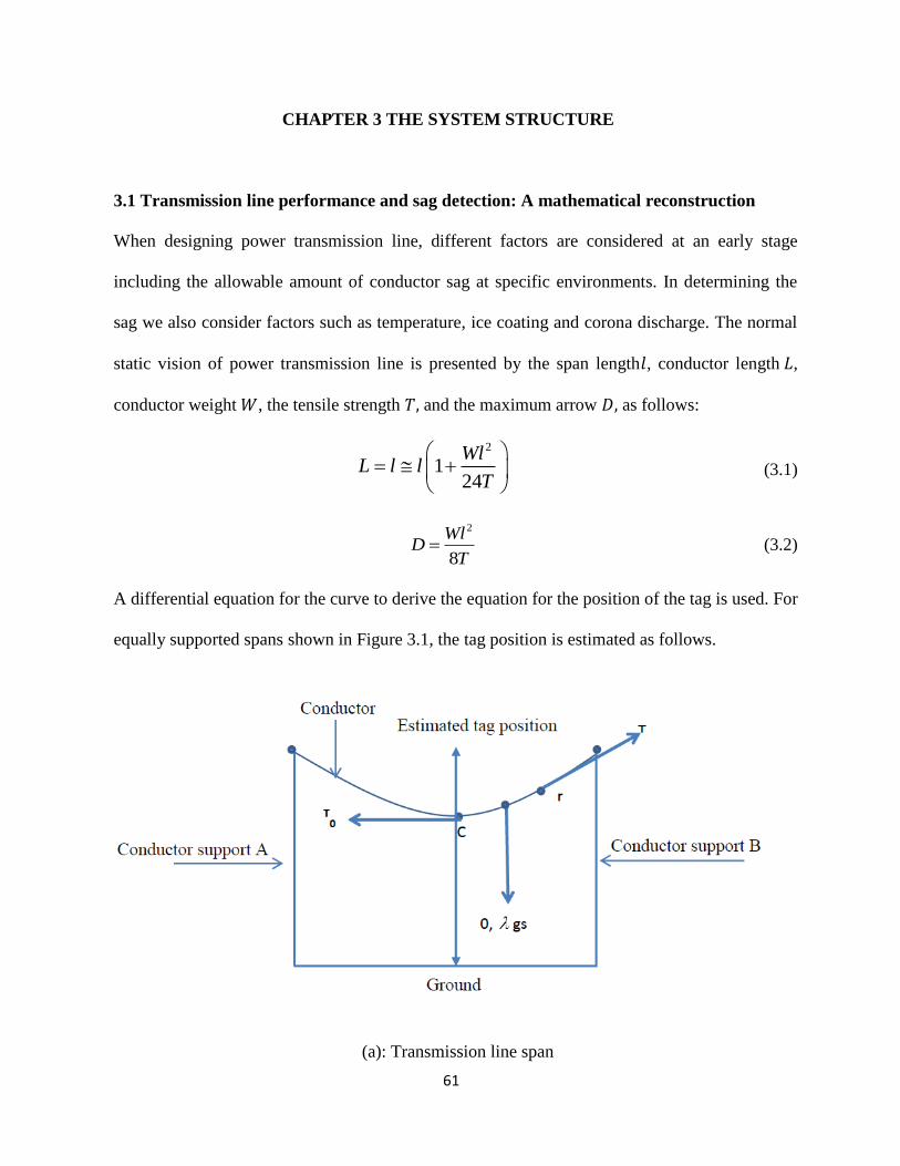
61
CHAPTER 3 THE SYSTEM STRUCTURE
3.1 Transmission line performance and sag detection: A mathematical reconstruction
When designing power transmission line, different factors are considered at an early stage
including the allowable amount of conductor sag at specific environments. In determining the
sag we also consider factors such as temperature, ice coating and corona discharge. The normal
static vision of power transmission line is presented by the span length𝑙, conductor length 𝐿,
conductor weight 𝑊, the tensile strength 𝑇, and the maximum arrow 𝐷, as follows:
2
124
WlL l l
T
(3.1)
2
8
WlD
T (3.2)
A differential equation for the curve to derive the equation for the position of the tag is used. For
equally supported spans shown in Figure 3.1, the tag position is estimated as follows.
(a): Transmission line span
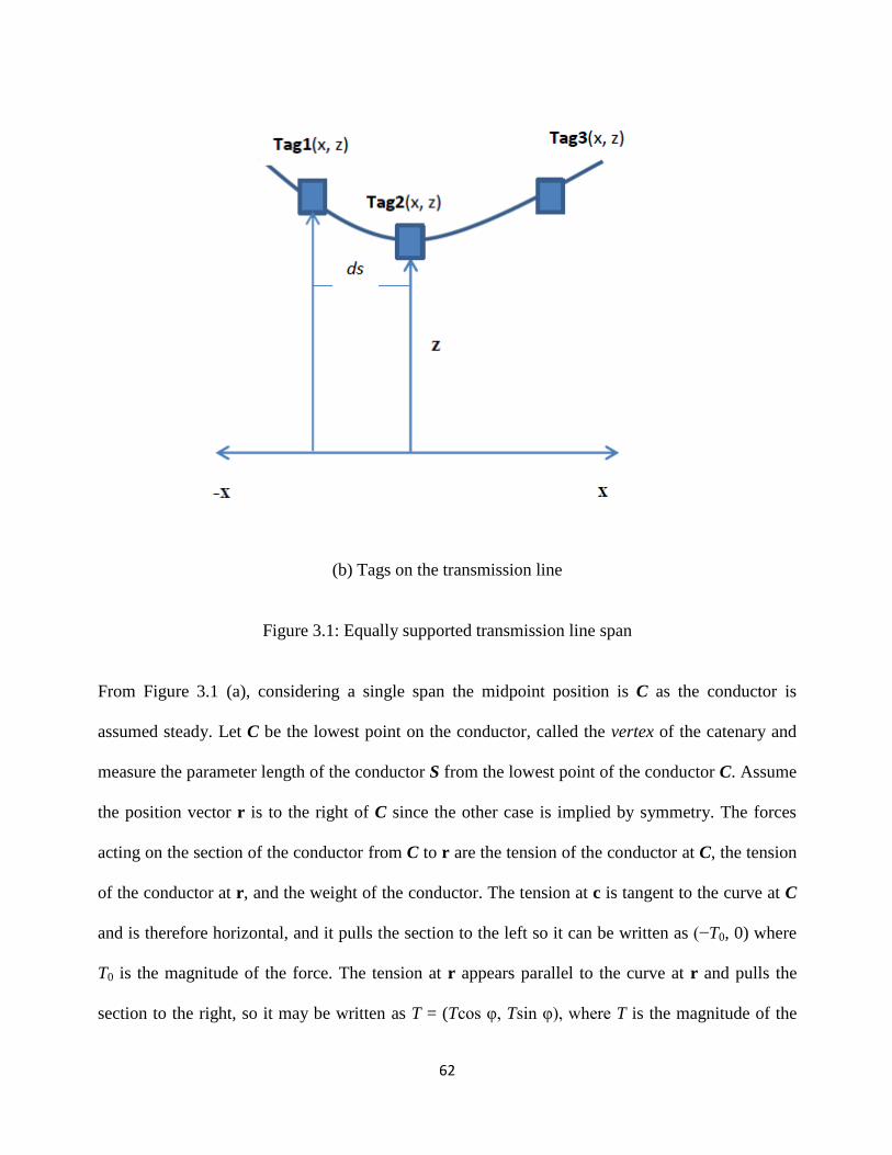
62
(b) Tags on the transmission line
Figure 3.1: Equally supported transmission line span
From Figure 3.1 (a), considering a single span the midpoint position is C as the conductor is
assumed steady. Let C be the lowest point on the conductor, called the vertex of the catenary and
measure the parameter length of the conductor S from the lowest point of the conductor C. Assume
the position vector r is to the right of C since the other case is implied by symmetry. The forces
acting on the section of the conductor from C to r are the tension of the conductor at C, the tension
of the conductor at r, and the weight of the conductor. The tension at c is tangent to the curve at C
and is therefore horizontal, and it pulls the section to the left so it can be written as (−T0, 0) where
T0 is the magnitude of the force. The tension at r appears parallel to the curve at r and pulls the
section to the right, so it may be written as T = (Tcos φ, Tsin φ), where T is the magnitude of the

63
force and 𝜑 is the angle between the curve at r and the x-axis. Finally, the weight of the conductor
is represented by (0, −λgs) where λ is the mass per unit length, g is the acceleration of gravity and s
is the length of conductor between C and r. The path of the conductor route is presented by a
parametric equation of a curve through the equation expressing the coordinates of the point of the
curve;
( , ) ( ( ), ( ))r x y x s y s (3.3)
dru
ds Where 𝑢 is a unit tangent vector (3.4)
Since our conductor is assumed to be equilibrium
0cosT T (3.5)
sinT gp (3.6)
0
tandy gs
dx T
(3.7)
Putting 𝑎 as,
0Ta
g (3.8)
Bearing in mind that the conductor weight is equal in magnitude as the tension at point C
(0, )gs . It is simpler to define the curve by,
dy s
dx a (3.9)
Solving the differential equation above, the arc length is determined by,
222 2
21
a sds dx dy dy
dx dx dx a
(3.10)
Then

64
2 2
1dx a
dsds a sdx
(3.11)
2 2
dy
dy sdxdsds a sdx
(3.12)
Integrating this equation gives,
2 2y a s (3.13)
Where is an integral constant
If β = 0 then,
2 2 2 2 2,y a s y a s (3.14)
The integral expression of dx
dsis given by,
1sinh ( )s
x aa
(3.15)
Where is an integral constant
The integral of dx
dsis
1sinh ( ), sinh( )s x
x a s aa a
(3.16)
Shifting the y-axis position the angle α = 0,
1sinh ( ), sinh( )s x
x a s aa a
(3.17)
Considering the temperature effect which escalates the stress σ, of the conductor, the thermal
expansion is noted, in that

65
22
2 2
2
0
1 1 ,
1o
ds dy Ws dqor dx
dx dx T w q
T
(3.18)
Where 𝑠 is the arc length in this case and other parameters remain unchanged. When integrating
both sides we find that,
2 2
2
0
1
dsdx
W s
T
(3.19)
10
0
T Wsx sih C
W T
(3.20)
Assuming the conductor becomes elastic due to the sigma factor then we have the linear elastic
such that E . Where is the stress, E is the constant of modulus elasticity and is the
strain. If 𝑆 is the length then,
1T
S y pE
(3.21)
In this case 𝑝 is the natural length of a section of a conductor, 𝑇 becomes the tension applied and
𝐸 the constant then,
1ds T
ydp E
(3.22)
So the elastic conductor curve can be derived from the vertical tension T and the horizontal
tension 0T such that for unchanged length we say,
0cosT T (3.23)
0sinT gp (3.24)

66
Where 0 is the mass per unit length of the conductor without tension and g is the gravitational
acceleration.
Re-writing this formulae
0
0
tangpdy
dx T
(3.25)
2 2
0, ( )and T T gp
The mass of the conductor, in nature is denoted as 0 .
Let
0
0
Ta
g (3.26)
Then
2 20tan ,Tdy p
T a pdx a a
(3.27)
Since
0sin ,gpdy
ds T
(3.28)
0cosTdx
ds T (3.29)
Evaluating in terms of natural length
0 0
2 21
T Tdx ds a
dp T dp Ea p
(3.30)
And substituting (3.26) to (3.31) we have,
0 0 0
2 2
1 1gp T p T pdy ds p
dp dp T a T E Eaa p
(3.31)

67
Integratingdy
dp, to obtain 𝑥 and 𝑦 we obtain,
1 0sinhTp
x a pa E
(3.32)
And
2 2 20
2 a
Ty a p p
E (3.33)
When considering the wind pressure 𝑞 and the conductor with the ice weight iw , the size of the
conductor thickness 𝑡. We can have the resultant force acting on the line 𝑊, where;
2 2( )tW q W W (3.34)
The tensile strength during the construction and the tensile strength in adverse conditions cT are
also taken into account then, and could be found as follows;
2 22 23 2
20
24 24
aa c
c
W l EW lT T E at T
T
(3.35)
Assuming the length of the cable is 𝑋 at Figure 3.1 (b) as it lies between two points ( , )x z and
( , )x z . The height of the cable can be determined from the point of its potential energy as it lies
on the 𝑥𝑧 plane. With ( 0)z and 2X x satisfy the inequality. Assuming that 𝑑𝑚 is the mass,
𝑑𝑉 be the potential energy, mass density per unit length, g the gravitational velocity and ds the
arc length.
( ) ( )dV dm gz ds gz (3.36)
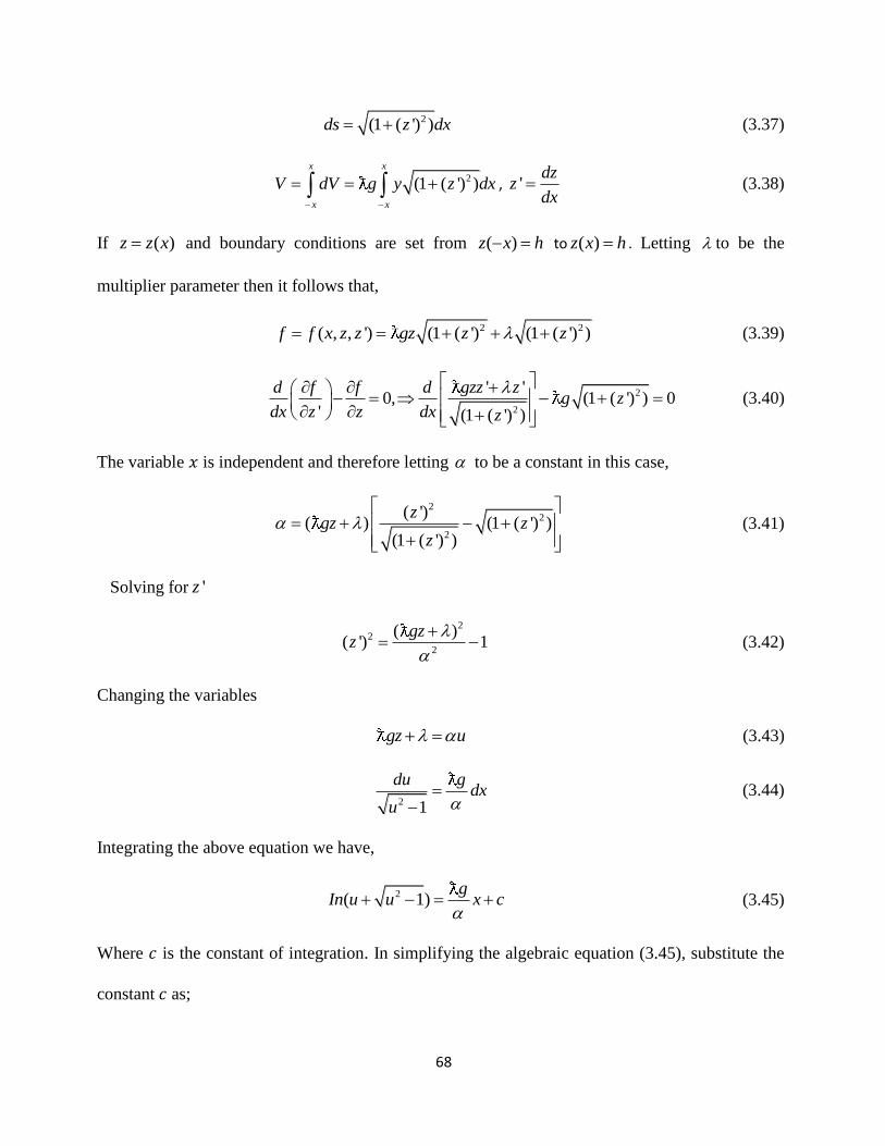
68
2(1 ( ') )ds z dx (3.37)
2(1 ( ') )
x x
x x
V dV g y z dx
, 'dz
zdx
(3.38)
If ( )z z x and boundary conditions are set from ( )z x h to ( )z x h . Letting to be the
multiplier parameter then it follows that,
2 2( , , ') (1 ( ') (1 ( ') )f f x z z gz z z (3.39)
2
2
' '0, (1 ( ') ) 0
' (1 ( ') )
d f f d gzz zg z
dx z z dx z
(3.40)
The variable 𝑥 is independent and therefore letting to be a constant in this case,
22
2
( ')( ) (1 ( ') )
(1 ( ') )
zgz z
z
(3.41)
Solving for 'z
2
2
2
( )( ') 1
gzz
(3.42)
Changing the variables
gz u (3.43)
2 1
du gdx
u
(3.44)
Integrating the above equation we have,
2( 1)g
In u u x c
(3.45)
Where 𝑐 is the constant of integration. In simplifying the algebraic equation (3.45), substitute the
constant 𝑐 as;

69
gc
where,
c
g
(3.46)
is a new constant
( )cosh
gz g xu
(3.47)
Therefore the height of the tag can be represented by
( )( ) cosh
g xz z x
g g
(3.48)
Where
2 2(1 ( ') ) cosh sinh
x x
x x
gx gxX z dx dx
g
(3.49)
These estimations are aimed to improve the efficiency usage of high voltage transmission line
by using RFID sag monitoring system. The target is to promptly providing the grid operators
with the conductor ground clearance. When all these parameters for power transmission line are
examined, a particular attention is on how RFID system performs under environmental factors.
We first look at the operation of the system and attempted to locate it in an equal or unequal
spans of transmission line.
To do this, firstly data obtained from 132 KV line tension and current parameters at Lesotho
Electricity Corporation (LEC) was used in the depicted Figure 3.2, and used to view the rate of
change of conductor sag. The derived mathematical model is then used to generate Figure 3.3
and demonstrate the variation of conductor sag for different times of three day period from 01
April 2015 to May 2015. There is a very complex correlation that is exhibited between
conductor sag and current loading due to variable temperature conditions.
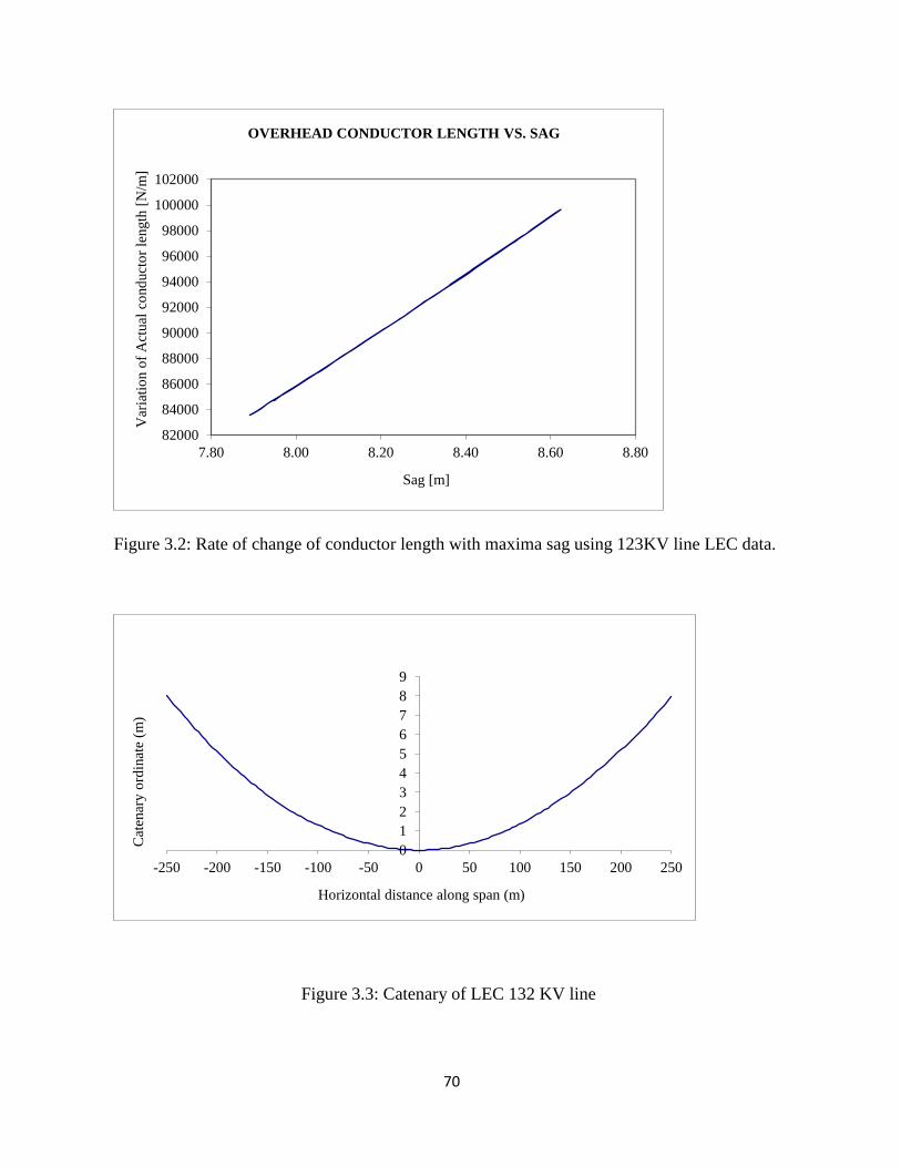
70
Figure 3.2: Rate of change of conductor length with maxima sag using 123KV line LEC data.
Figure 3.3: Catenary of LEC 132 KV line
82000
84000
86000
88000
90000
92000
94000
96000
98000
100000
102000
7.80 8.00 8.20 8.40 8.60 8.80
Var
iati
on o
f A
ctual
co
nd
uct
or
length
[N
/m]
Sag [m]
OVERHEAD CONDUCTOR LENGTH VS. SAG
0
1
2
3
4
5
6
7
8
9
-250 -200 -150 -100 -50 0 50 100 150 200 250
Cat
enar
y o
rdin
ate
(m)
Horizontal distance along span (m)
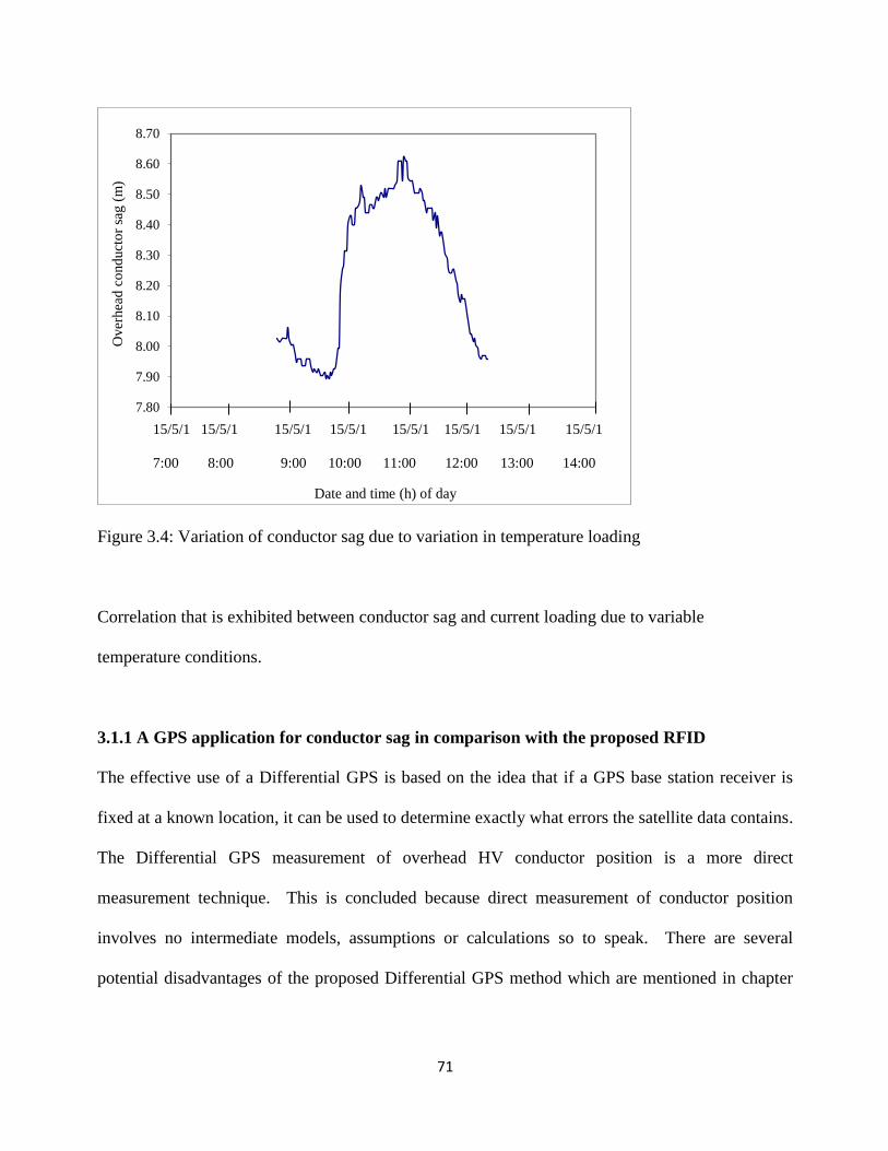
71
Figure 3.4: Variation of conductor sag due to variation in temperature loading
Correlation that is exhibited between conductor sag and current loading due to variable
temperature conditions.
3.1.1 A GPS application for conductor sag in comparison with the proposed RFID
The effective use of a Differential GPS is based on the idea that if a GPS base station receiver is
fixed at a known location, it can be used to determine exactly what errors the satellite data contains.
The Differential GPS measurement of overhead HV conductor position is a more direct
measurement technique. This is concluded because direct measurement of conductor position
involves no intermediate models, assumptions or calculations so to speak. There are several
potential disadvantages of the proposed Differential GPS method which are mentioned in chapter
7.80
7.90
8.00
8.10
8.20
8.30
8.40
8.50
8.60
8.70
Over
hea
d c
ond
uct
or
sag (
m)
Date and time (h) of day
15/5/1 15/5/1 15/5/1 15/5/1 15/5/1 15/5/1 15/5/1 15/5/1
7:00 8:00 9:00 10:00 11:00 12:00 13:00 14:00
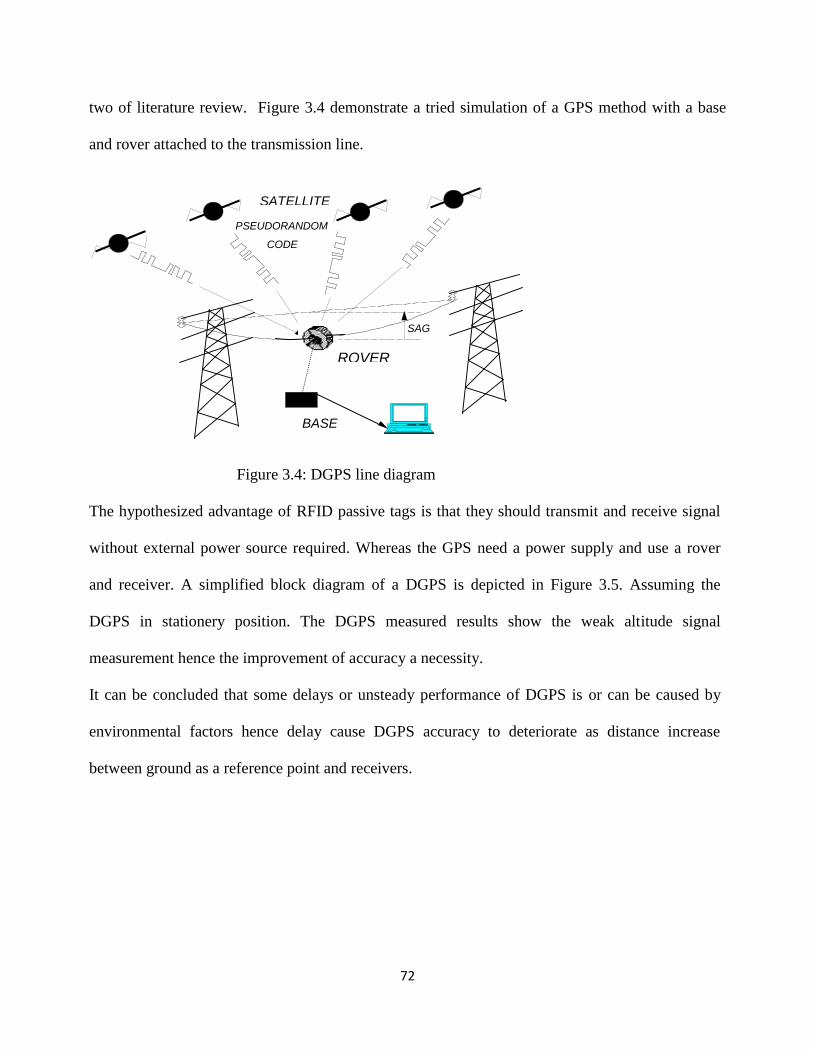
72
two of literature review. Figure 3.4 demonstrate a tried simulation of a GPS method with a base
and rover attached to the transmission line.
Figure 3.4: DGPS line diagram
The hypothesized advantage of RFID passive tags is that they should transmit and receive signal
without external power source required. Whereas the GPS need a power supply and use a rover
and receiver. A simplified block diagram of a DGPS is depicted in Figure 3.5. Assuming the
DGPS in stationery position. The DGPS measured results show the weak altitude signal
measurement hence the improvement of accuracy a necessity.
It can be concluded that some delays or unsteady performance of DGPS is or can be caused by
environmental factors hence delay cause DGPS accuracy to deteriorate as distance increase
between ground as a reference point and receivers.
ROVER
SATELLITE
SAG
BASE
PSEUDORANDOM
CODE
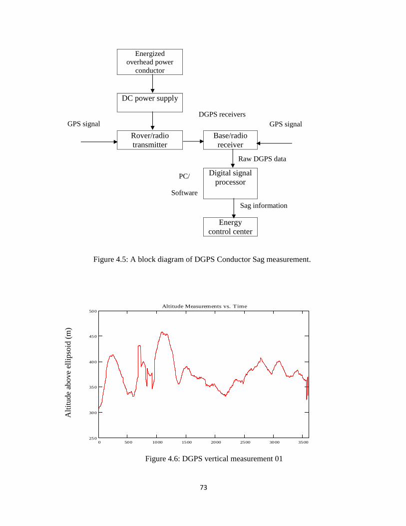
73
Energized
overhead power
conductor
DC power supply
Rover/radio
transmitter
Base/radio
receiver
Digital signal
processor
Energy
control center
Figure 4.5: A block diagram of DGPS Conductor Sag measurement.
Alt
itude
above
elli
pso
id (
m)
0 500 1000 1500 2000 2500 3000 3500250
300
350
400
450
500
Altitude Measurements vs. Time
Figure 4.6: DGPS vertical measurement 01
GPS signal
DGPS receivers
Sag information
Raw DGPS data
PC/
Software
GPS signal

74
Figure 4.7: DGPS vertical measurement distribution 02
Alt
itude
above
elli
pso
id (
m)
0 500 1000 1500 2000 2500 3000 3500350
360
370
380
390
400
410
420
430
Altitude Measurements vs. Time
Time (s)
Figure 4.8: DGPS vertical (z) measurement 03
0
200
400
600
800
1000
1200
1400
360 370 380 390
Sta
tist
ical
fre
quen
cy
Altitude above ellipsoid ( m )
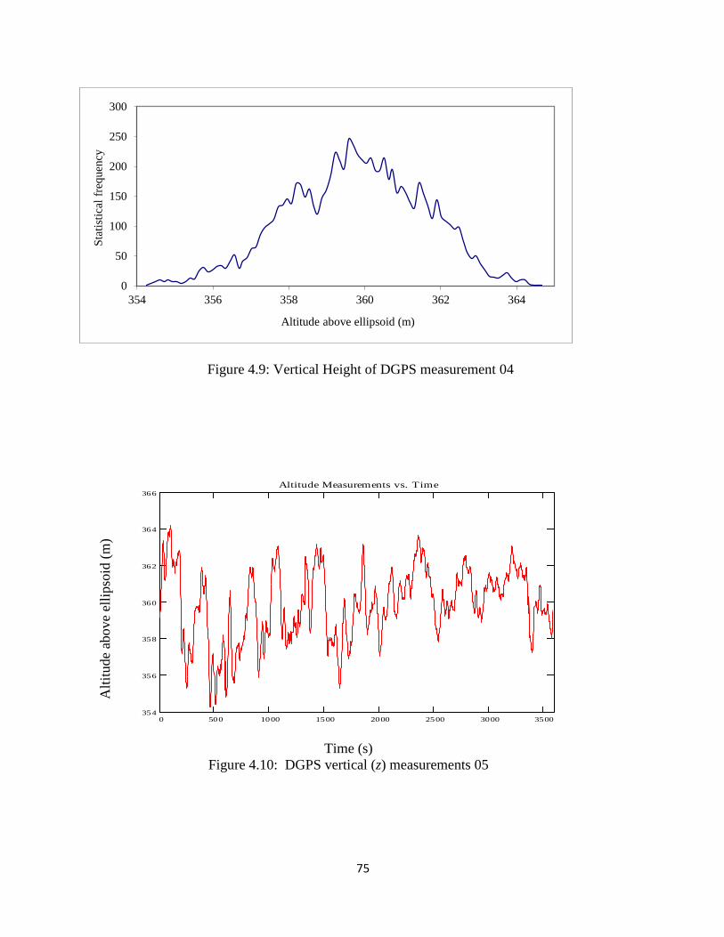
75
Figure 4.9: Vertical Height of DGPS measurement 04
Alt
itude
abo
ve
elli
pso
id (
m)
0 500 1000 1500 2000 2500 3000 3500354
356
358
360
362
364
366
Altitude Measurements vs. Time
Time (s)
Figure 4.10: DGPS vertical (z) measurements 05
0
50
100
150
200
250
300
354 356 358 360 362 364
Sta
tist
ical
fre
quen
cy
Altitude above ellipsoid (m)
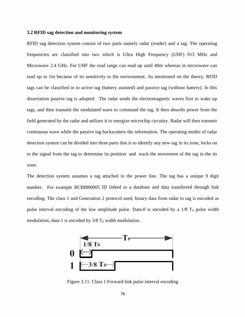
76
3.2 RFID sag detection and monitoring system
RFID sag detection system consist of two parts namely radar (reader) and a tag. The operating
frequencies are classified into two which is Ultra High Frequency (UHF) 915 MHz and
Microwave 2.4 GHz. For UHF the read range can read up until 40m whereas in microwave can
read up to 1m because of its sensitivity to the environment. As mentioned on the theory, RFID
tags can be classified in to active tag (battery assisted) and passive tag (without battery). In this
dissertation passive tag is adopted. The radar sends the electromagnetic waves first to wake up
tags, and then transmit the modulated wave to command the tag. It then absorbs power from the
field generated by the radar and utilizes it to energize microchip circuitry. Radar will then transmit
continuous wave while the passive tag backscatters the information. The operating modes of radar
detection system can be divided into three parts that is to identify any new tag in its zone, locks on
to the signal from the tag to determine its position and track the movement of the tag in the its
zone.
The detection system assumes a tag attached to the power line. The tag has a unique 9 digit
number. For example BCBBB0005 ID linked to a database and data transferred through link
encoding. The class 1 and Generation 2 protocol used, binary data from radar to tag is encoded as
pulse interval encoding of the low amplitude pulse. Data-0 is encoded by a 1/8 T0 pulse width
modulation, data-1 is encoded by 3/8 T0 width modulation.
Figure 3.11: Class 1 Forward link pulse interval encoding

77
Figure 3.12: Generation 2 forward link pulse interval encoding
The duration of data-0 is T0; the duration of data-1 is between 1.5 T0 and 2 T0. In class 1 protocol
radar talk to tag via the amplitude shift keying modulation from 30% to 100% depth. While in
Gen 2 protocol radar have to use double-sideband amplitude shift keying (DSB-ASK), single side
amplitude shift keying or phase reversal amplitude shift keying and the 80% to 100% modulation
depth.
Example of data linked to database
Time Tag ID Distance
22:45:08
22:45:08
22:45:08
22:45:09
22:45:09
22:45:09
BCBBB0005
BCBBB5002
BCBBB0026
BCBBB0004
BCBBB0002
BBBBB0000
19.2 m
0.5 m
31.6m
15.5m
3.1 m
8.8 m
Table 3.1: Example of data linked to database
3.2.1 Structure design of the monitoring system
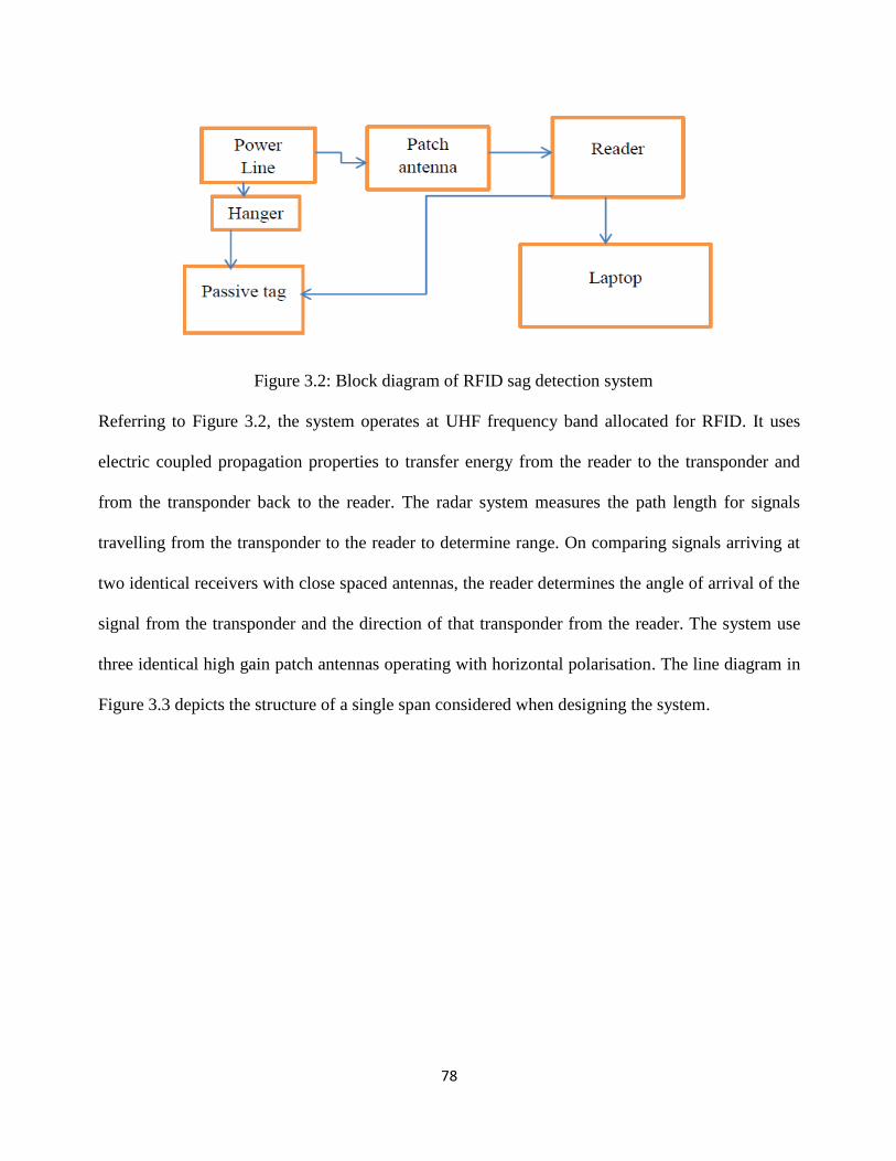
78
Figure 3.2: Block diagram of RFID sag detection system
Referring to Figure 3.2, the system operates at UHF frequency band allocated for RFID. It uses
electric coupled propagation properties to transfer energy from the reader to the transponder and
from the transponder back to the reader. The radar system measures the path length for signals
travelling from the transponder to the reader to determine range. On comparing signals arriving at
two identical receivers with close spaced antennas, the reader determines the angle of arrival of the
signal from the transponder and the direction of that transponder from the reader. The system use
three identical high gain patch antennas operating with horizontal polarisation. The line diagram in
Figure 3.3 depicts the structure of a single span considered when designing the system.

79
Figure 3.3: single line diagram for unequal supports with RFID sag detection system
3.2.1.1 Capacitance of transmission line
In high frequency circuits and long distance transmission lines capacitance C is actually
proportional to the charging current drawn from the field of the line. This is an important factor
when sag detection is done with RFID tag. Other variables such as inductance L, Voltage V
contribute to the nature of response which will be received from the tag. As a result the more
voltage applied to the line the more charge will be seen on the capacitor, which is predicted to be
one of the constraints in RFID tag performance.

80
Figure 3.4: Transmission line circuit
This relationship is predicted that charge will be proportionally to the voltage applied to the
conductor as seen by blue and the charge by red.
Figure 3.5: Capacitance charge voltage response
3.2.2 Principle of the monitoring system

81
One of the antennas is used for providing the energy field whereas the other two are used to receive
the weak signals for the receiver. The spacing of the receiver antennas is important for calculating
the angle of arrival. These antennas are 31 cm apart and the energising antenna 54cm from the right
receive antenna. It must be mentioned that two antennas work as sensors and the third antenna
work as an energiser which is mounted at the right.
The energising antenna is on the right behind the array and towards its direction of radiation so as
to complement the function of energy signal such that;
2( )fE f t dt
(3.50)
While the receive antennas are the centre antenna and the left hand antenna. Because the operation
principle of energizer antenna uses the function of energy signals it can be represented by the
signal expansion using a series of basic functions ( ( )n t ) because the response of a linear system
to a complex periodic signal can be found by linear superposition of the responses of simpler
inputs. Let be the time interval and nC the coefficient expansion, then,
1 1
1 10
( ) ( ) ( ) ( )
t t
m n m n
nt t
t f t dt c t t dt
(3.51)
The RFID radar is set to make two measurements on each signal received from each transponder in
its receiving zone - namely a range measurement and an angle of arrival. Taking the range
measurement with narrow bandwidth, the performance of the system will make this an outstanding
unique RFID instrument for sag detection. The system uses the same transponders that are used by
conventional RFID readers allowing RFID radar to monitor the same transponder simultaneously.
Light and radio waves travel at the speed of light, namely 300 000 000 meters per second. RFID
systems need to operate in a crowded RF spectrum, where other RFID systems, cell phones, radio
82
stations and other communication users have to share the available radio spectrum. RFID-radar
uses just 10 kilohertz of bandwidth to operate, meaning we are able to detect time differences only
as small as 0.1 milliseconds, or 0.0001 seconds. In this time the radio wave will travel 30
kilometers, or 30 000 meters or 3 000 000 centimeters; yet the radar is able to determine the range
of the transponder based on its received transmission to an accuracy of a few centimeters, or nearly
1 million times better than its basic time measuring properties. If conventional military radar
approach is employed and expecting to get centimeter precision, then the time of flight
measurement has to be done in the precision of 0.3pico seconds (.3*10-12) which would use
300GHz spectrum. RFID radar pays for this million times improvement in the timing accuracy of
the basic system by taking a longer time to determine the exact position. As a result it is well suited
to static situations where transponders are relatively stationary like suspended on the overhead
transmission line for sag detection. However developments are in progress to address the accurate
tracking of movement by adapting some of the principles of operation. The angle of arrival
measurement is virtually instantaneous and used in conjunction with range from a single measuring
location.
The system measures range by calculating the distance a signal from the transponder has travelled
to the reader. To acquire correct measurement the reader determines delays through the antennas
and time to travel through the cables and the amplifiers. The delay of the signals from the stick tags
is slightly different from that of the claymore tags hence the stick tags are very good in calibrating.
They have the same radiation pattern as a dipole but with the battery assistance for power usage.
The radar is able to resolve angles based on the 31cm spacing of the receive antennas of the
negative 30 degrees to positive 30 degrees. Should it happen that the transponder is beyond those

83
angles, that particular tag will be read and displayed with the negative angle. For the tag moving
from the left to right at 10 degrees per reading, the angles are displayed as follows:
Figure 3.5 Radar angle positioning in degrees
-30 degrees
-20 degrees
-10 degrees
0 degrees
10 degrees
20 degrees
30 degrees
-20 degrees ALIASED
-10 degrees ALIASED
84
The hanger used to suspend a tag from the transmission line under 11KV is a non-conductor strain
insulator. This is suspended about 2.3cm below the midpoint of the span. The midpoint of the span
where the sag is at lower point is determined by the sag equation;
2
8
wlD
T (3.52)
The D value is regarded as the lowest point caused by the weight of the conductor. For equal spans
this becomes the target point of the tag placement which is within the reader zone.
3.2.3 Selection of tags
A common tag implementation consists of an electronic microchip that stores data and executes the
tag’s functionality, an antenna that performs the function of receiving and transmitting RF energy,
a tag powering circuit that utilizes the RF power from the reader to power up the microchip, and
substrate into which the whole tag is built upon. The tag integrated circuit controls the tag
operations according to the reader’s commands and the communication protocol. Tag antenna
receives readers continuous wave (CW) during the readers powering up phase. The tag powering
up circuit rectifies this CW signal from the reader and further delivers it to its integrated circuit
(IC). Powering up phase of the reader transmission is followed by the command transmission phase
in which modulated RF is sent by the reader as command signal. The powered up tag IC executes
the reader’s command. After the reader has transmitted its command, it again starts to broadcast a
continuous field again which the tag will modulate and backscatter again as its response to the
reader’s command. The modulation then is produced by switching the tag’s antenna matching. The
Figure 3.6 shows the communication principle of tag to reader.

85
Figure 3.6: communication principle of a tag
The communication of tag, as response of the tag to the reader’s query identity (ID) command
depends on whether reader is operating in global scroll or inventory mode. The query ID command
format from the reader depends upon these modes and depending upon which format is used in the
reader data field, the tag response will take one of the two possible forms. The global scroll
command is intended to identify one tag at a time and the tag response to this command is
generated in the form of tags identification code in the wheel, which includes both the tag’
electronic product code (EPC). In case of inventory mode of the reader goes through all possible
code combinations with the minimum number of readings using an anti-collision algorithm. Each
reply of the tags includes a 15bit part of its EPC defined in the reader’s command code. Passive
transponders are in a form of credit card sized offering the range up to 18m. Battery assistant does
not operate on the dedicated frequency. They operate over the frequency range of 100 MHz, and
allow many types of radar systems to determine their range at the same instant, even if radars are
operating on slightly different frequencies. These transponders do not radiate any energy and are
not transmitter type of devices.

86
Claymore types are active tags since they are battery assisted. They are generally mounted on a
large piece of plastic and are made to be attached to a large item, such as a container. They use the
nearness of the large item as part of the antennas to focus additional energy onto the sensitive part
of the antenna and in doing so, is thereby increasing the range. These transponders have a direction
of radiation marked on the transponder. The advantage of active tags is that they provide longer
read range and can perform other functions apart from the reader’s request, although they are
costly.
Stick type transponders and credit card type transponders radiate energy equally around the center
longitudinal axis. These are passive tags which have an advantage of not requiring any external
power source like active tags. In the dissertation credit card passive are used to test the system
operation in different conditions. Clay more and stick tags are used to determine the precision
measurement and detection errors.
3.2.4 Backscattering of the system
The major components of a backscattering passive system are readers, tags and an application host.
RFID radar mainly comprises of a set of antenna, a radio interface, a control unit and a powering
unit. The antenna performs the function of transmitting and receiving the electromagnetic energy
used for communication and powering the tags, within its range in that a signal transmitted is finite
average power, 𝑃. For signal 𝐹(𝑡) at time interval from 𝑡1 to 𝑡2.
22
2 1 1
1( ) .
t
t
P f t dtt t
(3.53)
It satisfies that
87
22
2
10 lim ( )
T
TT
f t dtT
(3.54)
The radio interface performs the job of detection, modulation, and demodulation of the RF signal.
The control unit executes the communication protocol with the tags and interprets the data received
from the tags. In performing all the above-mentioned functionalities, the reader communicates with
the tags within range as directed by the application host and reports the results to the host.
3.2.5 Interference problem
Passive UHF RFID system operates by a very steady manner of energizing signal which is received
by the tag, converted to direct current (DC) power which powers the tag. This is a carrier wave
signal that has minimal modulation and causes virtually no interference to the system on
frequencies adjacent to the operating one. As the data from the tag to the reader sent back by
backscattering modulation in such that antenna impedance of the tag is altered by the data to be
transmitted, causing differing amounts of energy to be reflected by the tag back to the reader. This
in most cases result the data to be reflected at virtually the same frequency as the energizing field
and therefore cannot be detected to any other equipment that the reader provide the energy field. As
the energy from the transmitter leaves the antenna it travels away at the speed of light, in various
directions at instant. The Figure 3.7 presents area surface of 1m and 2m of antenna sphere.

88
Figure 3.7: Area surface of the antenna sphere
The bigger shaded area marked in the Figure 3.7 is the surface area of the cell on 2m sphere and the
other small shaded area is the surface area of a cell on a 1m antenna sphere. By the time the energy
gets 1m away from the antenna, the Power density DP will be as follows:
24
TD
PP
r (3.55)
Where TP power transmitter and 𝑟 is the sphere radius of 1meter.
Compared to the old historic tags or transponders systems, UHF tags operate over ranges that are
doubling the wavelength of their operating frequency. The Figure 3.8 shows signals arriving at a
point without any shifting phase difference.
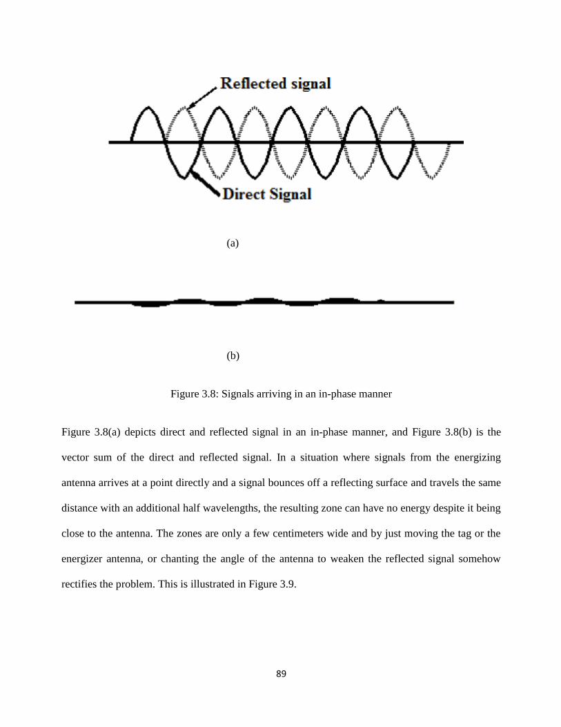
89
(a)
(b)
Figure 3.8: Signals arriving in an in-phase manner
Figure 3.8(a) depicts direct and reflected signal in an in-phase manner, and Figure 3.8(b) is the
vector sum of the direct and reflected signal. In a situation where signals from the energizing
antenna arrives at a point directly and a signal bounces off a reflecting surface and travels the same
distance with an additional half wavelengths, the resulting zone can have no energy despite it being
close to the antenna. The zones are only a few centimeters wide and by just moving the tag or the
energizer antenna, or chanting the angle of the antenna to weaken the reflected signal somehow
rectifies the problem. This is illustrated in Figure 3.9.

90
Figure 3.9: The shifting of the energizer angle
The same situation can possible be seen in a case of signal back from the tag to the sensing
antenna. For this phenomenon to occur a good reflecting surface is needed. In the scenario where
the tag and the reader are moving relative to each other, the hole problem is not significant as even
though it might be in few times where the tag is in holes, with relative motion which will cause the
location of the holes to move and power will be restored to the tag.
3.2.6 Effect of mounting the antenna
As the antennas radiates and receive electromagnetic energy into the air. The property of the
resulting signal is polarization. Here in Figure 3.10, we illustrate two polarizations examined in our
antenna study.
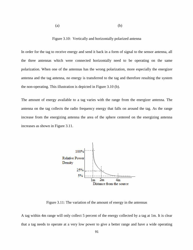
91
(a) (b)
Figure 3.10: Vertically and horizontally polarized antenna
In order for the tag to receive energy and send it back in a form of signal to the sensor antenna, all
the three antennas which were connected horizontally need to be operating on the same
polarization. When one of the antennas has the wrong polarization, more especially the energizer
antenna and the tag antenna, no energy is transferred to the tag and therefore resulting the system
the non-operating. This illustration is depicted in Figure 3.10 (b).
The amount of energy available to a tag varies with the range from the energizer antenna. The
antenna on the tag collects the radio frequency energy that falls on around the tag. As the range
increase from the energizing antenna the area of the sphere centered on the energizing antenna
increases as shown in Figure 3.11.
Figure 3.11: The variation of the amount of energy in the antennas
A tag within 4m range will only collect 5 percent of the energy collected by a tag at 1m. It is clear
that a tag needs to operate at a very low power to give a better range and have a wide operating

92
voltage to allow it to work close to energizer antenna. It can be conclude that at a very close range
a tag might overload and stop working.
3.2.7 Effect of attaching the tag on the conducting or non-conducting material
The tags used in the proposed system, credit type passive tags are used which can read up until
18meters range. When UHF radio wave is travelling through medium and encounter a surface of a
different material that is large compared to the wavelength of the radio wave, some of the energy is
reflected at the interface and some is transmitted through the new medium. Whenever the radio
signal travelling through medium encounters an object with a different dielectric constant, it causes
some of the energy to reflect therefore thwarting it not to reach the intended tag. The objects are to
be sizable compared to the wavelength of the signal (32cm at 915MHz) for the impact to be
notable. The reflection from the items such as wood, paper, cement, and ceramic is similar to the
reflections got from the conducting materials such as steel conductor or water. The sensitivity of
the tag for a dipole type antenna, operating at 915MHz, would be 132𝑐𝑚2.
3.2.7.1 Effect of attaching the tag on the conducting material
At the surface of the metal where the signal that travel through the air meets the metal conductor,
the signal is reflected from the metal back towards the reader and this signal has the opposite phase
angle to the incoming signal which then cancels the incoming signal at the surface. A few
millimeters away from the metal conductor a signal exists and can initiate a talk with the tag. The
Figure 3.12 shows the impact of mounting the tag at a small distance away from the metal
conductor, using some spacing material that has a dielectric constant similar to air.
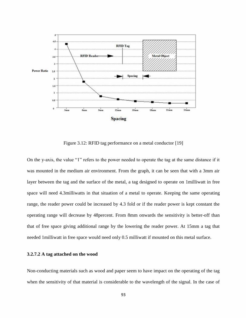
93
Figure 3.12: RFID tag performance on a metal conductor [19]
On the y-axis, the value “1” refers to the power needed to operate the tag at the same distance if it
was mounted in the medium air environment. From the graph, it can be seen that with a 3mm air
layer between the tag and the surface of the metal, a tag designed to operate on 1milliwatt in free
space will need 4.3milliwatts in that situation of a metal to operate. Keeping the same operating
range, the reader power could be increased by 4.3 fold or if the reader power is kept constant the
operating range will decrease by 48percent. From 8mm onwards the sensitivity is better-off than
that of free space giving additional range by the lowering the reader power. At 15mm a tag that
needed 1milliwatt in free space would need only 0.5 milliwatt if mounted on this metal surface.
3.2.7.2 A tag attached on the wood
Non-conducting materials such as wood and paper seem to have impact on the operating of the tag
when the sensitivity of that material is considerable to the wavelength of the signal. In the case of

94
these materials, the reflection from the surface is not so bigger in such that it require much greater
power for the tag that is close to the surface and at some instance at further distances, they do not
give sensitivities that are much better than that which we achieve in free space. This performance is
shown on Figure 3.13.
Figure 3.13: Tag performance on the wooden object [19]
3.2.7.3 Mounting a tag on a wet body
It is imperative also to examine whether the blood flow in human body, which is also an electrical
path to the ground, could possibly have the impact on tag performance. This needs a further study
in future. However Figure 3.14 shows a graph that depicts a performance.

95
Figure 3.14: RFID tag performance on a human body [19]
Figure 3.14 show that the high water content body or flesh which is close to the tag impacts the
operation of the tag. Hot sweating bodies kill the RF signals close to the skin.

96
3.2.7.5 Tag on the paper
Figure 3.15: Tag performance on piled stack of papers [19]
The paper has a different dielectric constant from that of air meaning that at the interface between
the paper and the air, energy will be lost as it will be reflected away. The energy would then travel
through the paper to the tag. In Figure 3.15, we can compute this tag performance as if it is on air
by attaching it on the paper. From then it is seen that, at about 10mm to 50mm below the surface of
the paper piles, the energy goes between, 3.5 to 4.5 higher than that needed for the freely spaced
tag.

97
3.2.8 RFID tag positioning in three dimensions
(a) Reader with three patch antennas and one energizer
(b) Intersection of surface circles
Figure 3.16: Three dimension tag positioning

98
From Figure 3.16, the intersection of the three circles is found by formulating the equation for
three surfaces and solving for the unknown variables of 𝑥 𝑦 and 𝑧. From Figure 3.16 (a) we have
𝑥 as the horizontal plane, 𝑦 the vertical plane, and 𝑧 the third dimension. The formation is in
such that one point is at the origin and another point is on the 𝑥 axis. To find the third dimension
of the tag position, three receiving antenna are used. This process is simplified having the center
of the circle placed on the 𝑧 = 0 plane. The radius of the circle is denoted by 𝑟, the diameter 𝑑 and
𝑃 the circle. The first circle is represented by,
2 2 2 2
1r x y z (3.56)
Establishing the second circle we have,
2 2 2 2
2 ( )r x d y z (3.57)
The radius of the third circle is then written in terms of the coordinates(𝑖, 𝑗), 𝑖 is the horizontal
vector of P3 and 𝑗 is the vertical vector of P3.
2 2 2 2
3 ( ) ( )r x i y j z (3.58)
To obtain 𝑥 we subtract equation (3.54) from (3.53),
2 2 2
1 2
2
r r dx
d
(3.59)
Assuming that the first circles intersect at more than one point then we have
1 2 1d r r d r (3.60)
Substituting equation (3.56) in to (3.53), we have
2
2 2 2
1 22 2 2
1 24
r r dy z r
d
(3.61)
Re-writing equating (3.53) in terms of 𝑧 we have
2 2 2 2
1z r x y (3.62)
99
Substituting (3.59) in to (3.55)
2 2 2 2 2 2 2 2 2
1 3 1 3( )
2 2
r r x x i j r r i j iy x
j j j
(3.63)
Having found x and y, the z-coordinate is found by rearranging the formula for the first circle.
2 2 2
1z r x y (3.64)
3.2.9 Triangulation Method
Based on the accuracy features of the RFID radar system, i.e. low absolute accuracy but high
relative accuracy, triangulation method is proposed making use of multi-station
measurements. To reduce the cost, only a pair of receiving and sending antennas is needed.
The receiver is moved to imitate multi-station radar system. Four measurements are made
for positioning a tag. Complete 3D coordinates are calculated which high accuracy, which
are valuable to evaluate the line to line and line to environment clearances. By detecting
time of flight RFID radar has the ability to calculate the distance between the station and
tags. For multi-station system the location of tags can be calculated by triangulation method.
In fact, it is difficult for current technology to measure tiny time unit, such as picoseconds
that the signal travelled between a station and a tag with ten meters distance. The time spent
by individual tag to respond into the reader instruction is also different. Therefore the range
measurement is not accurate. The method rely on the signal strength has the similar problem
because the environment factors may affect the attenuation. RFID have significant when
measure absolute distances (about half meter errors), however, may have much better
accuracy (millimeter errors) for relative distance. According to this feature of RFID system,
this research also detects the tag position by moving the reader for relative distance
measurement and then using triangulation method to calculate the position.

100
Figure 3.17: Triangulation of the proposed method
Figure 3.17, depicts the principle of the proposed method. In this method, tag T1 is stuck on a
power line, the receiving antenna moves on ground points O, P1, P2 and P3. If assume O is the
origin, then P1 and P2 are located on x-axis, P3 is on y-axis. The positions of P1, P2 and P3 can be
exactly measured. The distances between T1 and these measures points are measured. According to
the cosine theorem of triangles, in 1 1TOP , we have;
2 2 2
1 1 1 1 22 cosra r a r (3.65)
2 2 2
1 1 2
1 1
cos2
r a r
r a
(3.66)
Considering triangle 1 2TOP
2 2 2
1 1 2 1 1 2 32 ( )cos ( )r a a r a a r (3.67)

101
2 2 2
1 1 2 3
1 1 2
( )cos
2 ( )
r a a r
r a a
(3.68)
To be noted that the absolute values of 1 2 3, ,r r r and 4r cannot be accurately measured. Fortunately
the differences between them are much more reliable, such that:
1 2 1r r r (3.69)
2 3 2r r r (3.70)
4 4 1r r r (3.71)
3 1 1 2r r r r (3.72)
Substitute equation (3.67) to equation (3.65), one gets
2 2 2
1 1 2 1 1 2
1 1 2
( ) ( )cos
2 ( )
r a a r r r
r a a
(3.73)
From equation (3.63) and equation (3.73),
2 2 2 2 2 2
1 1 2 1 1 2 1 1 2
1 1 1 1 2
( ) ( )
2 2 ( )
r a r r a a r r r
ra r a a
(3.74)
1r Can be derived as follows
2 2
1 2 1 2 2 1 1 1 1 21
1 2 2 1
( ) (2 )
2( )
a a a a a r a r r rr
a r a r
(3.75)
2 2
1 1 2 1 1 2
1 1 2
( ) ( )arccos
2 ( )
r a a r r r
r a a
(3.76)
From Equation (3.68) we have
4 1 4r r r (3.77)
In 1 3TOP

102
2 2 2
1 4
1
cos2
r b r
rb
(3.78)
2 2 2
1 4
1
cos2
r b rarc
rb
(3.79)
Since the Cartesian coordinates are convenient to calculate the distance to ground and the distances
between power lines, the derived position is converted to 1( , , )T x y z by the following equations.
1 cosx r (3.80)
1 cosy r (3.81)
2 2 2
1z r x y (3.82)
z is the distance from the power line to ground. The tag stores the information of which phase
power line it is sticking, so by the coordinates of tags it is easy to calculate the distances between
the power lines. A trilateration simulation is tried with three tags at different positions in Figure
3.18.
Figure 3.18: 2D trilateration simulation

103
Location of tag 1 on power
line; coordinates: [-2, 2]
Location of tag 2: [2, 1]
Location of tag 3: [-1, -2]
Figure 3.19: 3D trilateration simulation
Location of tag 1:
[-2, 2, 2]
Location of tag 2:
[2, 1, -1]
Location of tag 3:
[-1, -2, 2]
Location of tag 4:
[3, 3, 3]
Although tags are located at different heights, radar still identifies them correctly in both sides. Test
1 was viewed at the measurement of 7.5 meters. Test 2 at 1m, test 3 at 9m, and test 4 at
approximately 5m. As Figure 3.20, depict the results are non- consistent yet some are closer
to actual approximated measurable values. It can be seen that test 3 produce the most accurate
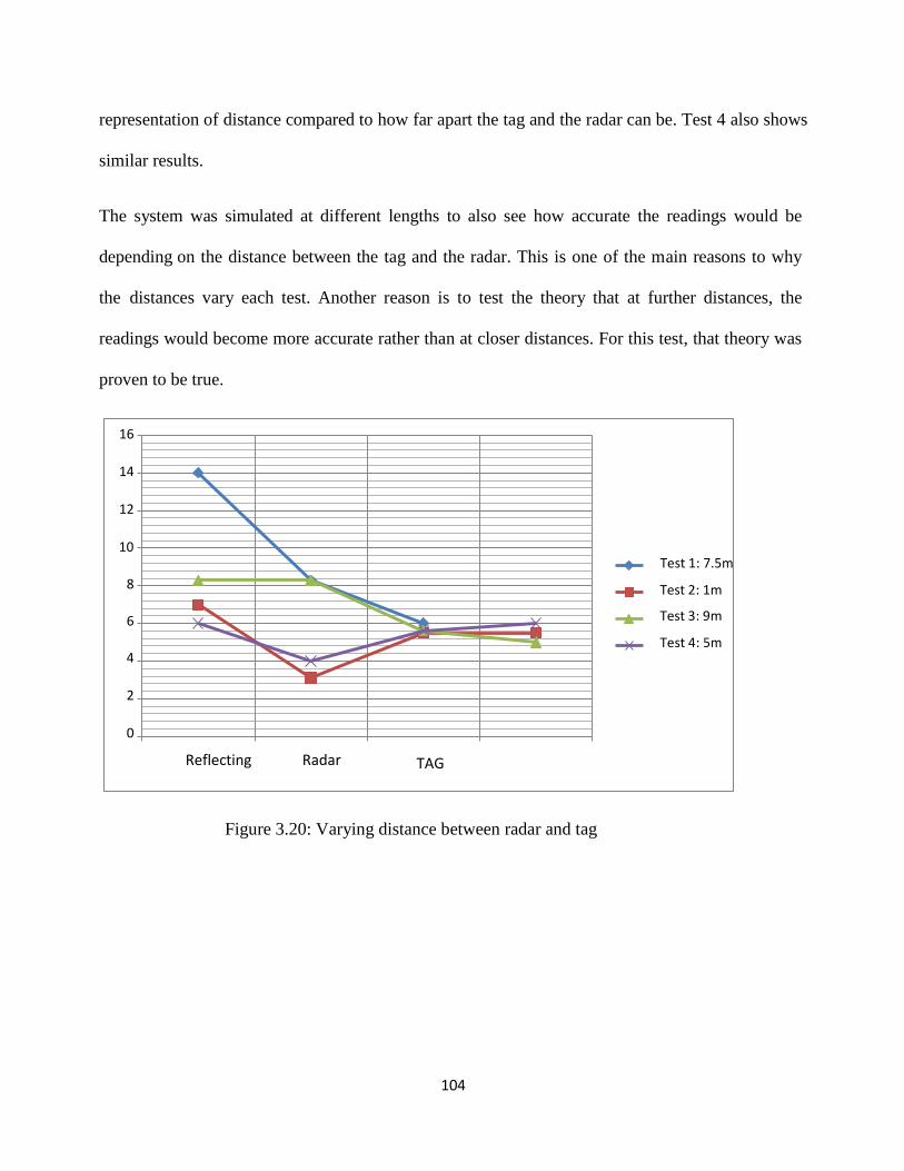
104
representation of distance compared to how far apart the tag and the radar can be. Test 4 also shows
similar results.
The system was simulated at different lengths to also see how accurate the readings would be
depending on the distance between the tag and the radar. This is one of the main reasons to why
the distances vary each test. Another reason is to test the theory that at further distances, the
readings would become more accurate rather than at closer distances. For this test, that theory was
proven to be true.
16
14
12
10
Test 1: 7.5m
8 Test 2: 1m
6 Test 3: 9m
Test 4: 5m 4
2
0
Reflecting Radar TAG
Figure 3.20: Varying distance between radar and tag

105
Figure 3.21: Distance between radar and tag
3.2.9.1 Summery of the proposed RFID sag monitoring system
The proposed system has the capability to monitor sag as long as the tag is present within the
radar zone, by moving the antenna receivers up to 30 degrees. The performance of the system
virtually depends on the amount of power a tag receives. This means that for a better
performance battery assisted tags are needed. Although passive tags gain advantage over the
active tags by their long life span, their drawback is that they are easily affected by most of
environmental factors such as temperature, pressure, tension, and stress.
3.3 Evaluation of the proposed RFID sag monitoring system
Reflecting
0
2
4
6
8
10
12
14
1
6
Radar Tag
Tst1-1.8m
Tst1-2.6m
Tst1-3.7m
Tst1-4.8m
Tst1-2.0m
106
The designed radar system can operate in different modes depending on the required data
output. Acquisition mode is the method which we use to read tags in the reader field. There are
two distinct methods for reading tags that is global scroll and inventory. The choice of one
method over another depends on the application at hand.
Global scroll is the most primitive of tag identity (ID) reading operations. When a global scroll
command is issued, the RFID Radar sends a single command over the air to each tag. This
command is simply a request for any tag to immediately send back its ID to RFID reader.
There are advantages and disadvantages in this method. The command is very quick to execute
as it involves only one round trip between the reader and the tag. However, because the
command is so simple, problems arise if there is more than one tag in the field. At this point in
time, multiple tags will all receive the same command and will all send back their ID’s to the
reader at virtually the same time all together. A situation such as this makes it difficult for the
reader to discern individual ID’s among the general noise of them all. Typically one or two of
the closest tags will be decoded, but the majority will not be discerned due to collision.
On the other hand inventory command was examined. It is a full featured system for discerning
the ID’s of multiple tags in the field at the same time. This single high-level command
transforms itself into a complex series of reader-tag interrogations that eventually resolve
themselves into a single list of tags ID’s seen by the RFID reader. This method of interrogation
and evaluation of multiple tags seems to be opposite to the former hence anti-collision. These
algorithms are far more complex than the global scroll algorithm, requiring many more readers’
tags instructions.

107
Tag read mode was also examined in the research. There are two methods of reading the tags,
interactive mode and autonomous mode. In what (Misic J., 2009), call inter-active mode, the
controlling application issues a command to the reader to read the transponder. The command
always immediately returns with a list of tags in the reader’s field of view. On the other hand in
the case of auto-nomous mode, the reader constantly reads tags, and may initiate a conversation
with a network listener when certain events arise. Both methods are equally useful, although it is
easier and require less coding to work in interactive mode.
A reader operating in autonomous mode moves between several states such as waiting, working,
evaluation and notification. Movement from one state to the next may be initiated by an
expiration of a timer, a triggered event on the digital input lines, or changes to the Tag list.
Autonomous mode has a feature by which the tag list delivered has time stamps indicating the
instants at which the tags were detected. These can then be used to correlate the tag ID’s with
the corresponding sensor data.
Antenna sequence technique provides the readers to invariably support the use of multiple
antennas and allow selecting which antennas, in the order specified in the antenna sequence. The
reader cycles through static systems or multi static systems. Mono-static system readers have the
ability to transmit and receive RF signals on the same antenna port. Multi static system readers
on the other hand transmit and receive RF signals on separate antennas providing significantly
better sensitivity to weak tag backscatter signals. These readers may allow fixed antenna pairing
scheme or more flexible arbitrary combinations of transmit/receive antennas, giving better RF
coverage over a larger area in the front of the reader with fewer antennas.

108
4. ANALYSIS AND RESULTS
Comments on GPS
GPS is very different from RFID. While it also uses radio waves to transmit data, it does so
using, global positioning system of 24 satellites, as opposed to radar system. Radio waves sent
out from this system of satellites transmit their time and orbital data to receivers down on Earth.
Using the data from multiple satellites, receivers can then triangulate their position relative to
the satellites, and thus on the Earth's surface. GPS, thus, is best suited for tracking geographic
position not sag detection. Because of the sheer distance of the satellites, the signal is weaker
and is easier to jam, or even just not get a signal.
Comments on RFID
There are two types of RFID tags: active tags, which contain a battery and are constantly
transmitting data such as vital signs, passive tags, which require radar to create a signal in an
otherwise battery less device. There is a potential of battery assisted passive tag in future, which
may function as a hybrid of the two in that an external source will be required to activate the
battery function.
Efficiency of RFID
More efficiency is found in RFID. For a tag to receive power from the radar, the following link
is followed:
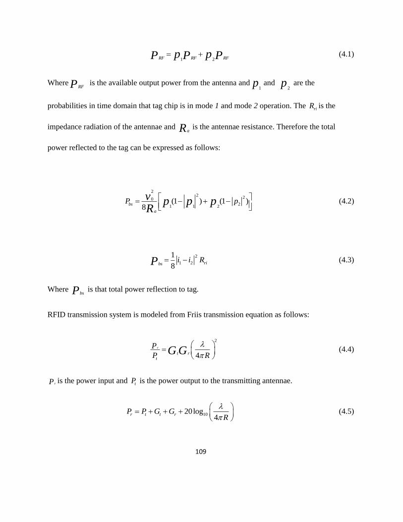
109
1 2RF RF RFp pP P P (4.1)
WhereRFP is the available output power from the antenna and
1p and
2p are the
probabilities in time domain that tag chip is in mode 1 and mode 2 operation. The riR is the
impedance radiation of the antennae and aR is the antennae resistance. Therefore the total
power reflected to the tag can be expressed as follows:
22
202
1 1 2(1 ) (1 )
8bs
a
P pv p p pR
(4.2)
2
1 2
1
8ribs
i i RP (4.3)
Where bsP is that total power reflection to tag.
RFID transmission system is modeled from Friis transmission equation as follows:
2
4
r
t rt
P
P RG G
(4.4)
rP is the power input and tP is the power output to the transmitting antennae.
1020log4
r t t rP P G GR
(4.5)

110
tG and rG are the antennae gains and obviously lambda is the wave length
22
1/2 1/2
0 0
10
1 1exp( ) ( ) exp( )
4
n
r t i i i
i i
P P G jkr G jkrr r
(4.6)
0G is the direct pathway antennae gain iG propagating antennae gain ( )i is the
reflection coefficient. Table 4.1 shows the summery of comparison between RFID and GPS.
Figure 4.1, depicts a simulation result of radar tag power received due to pole reflection.
RFID GPS
TAG has CPU I/O Its purpose is to define geographic position
on and above the earth surface. It consists of
three segments namely: user segment, control
segment and space segment.
RAM ROM
RADIO Tx/Rx
Energizer
Up to 96bit transmission Transmitting power is only 50 watts or less
Radar transmit power of 1Watt Very high orbit at 1 revolution in
approximately 12hrs
Radar receiver sensitivity -80dBm 24 satellites with 55 degrees
Radar antenna gain 1dBi-omini directional Prone to errors and needs a secondary GPS
namely DGPS
Tag power required 100 microwatt Broadcasting position and information on
two frequencies
Tag modular efficiency -20dB Signal weaker because of sheer distance
Method used to talk to the tag is modulated,
message format, commands and anti-
collision
Less power efficiency
Radio wave transmission of data Radio wave transmission of data

111
Figure 4.1: Radar received power
Figure 4.2: Tag received power
This concludes that the amount of signal power that the tag receives, after the command has
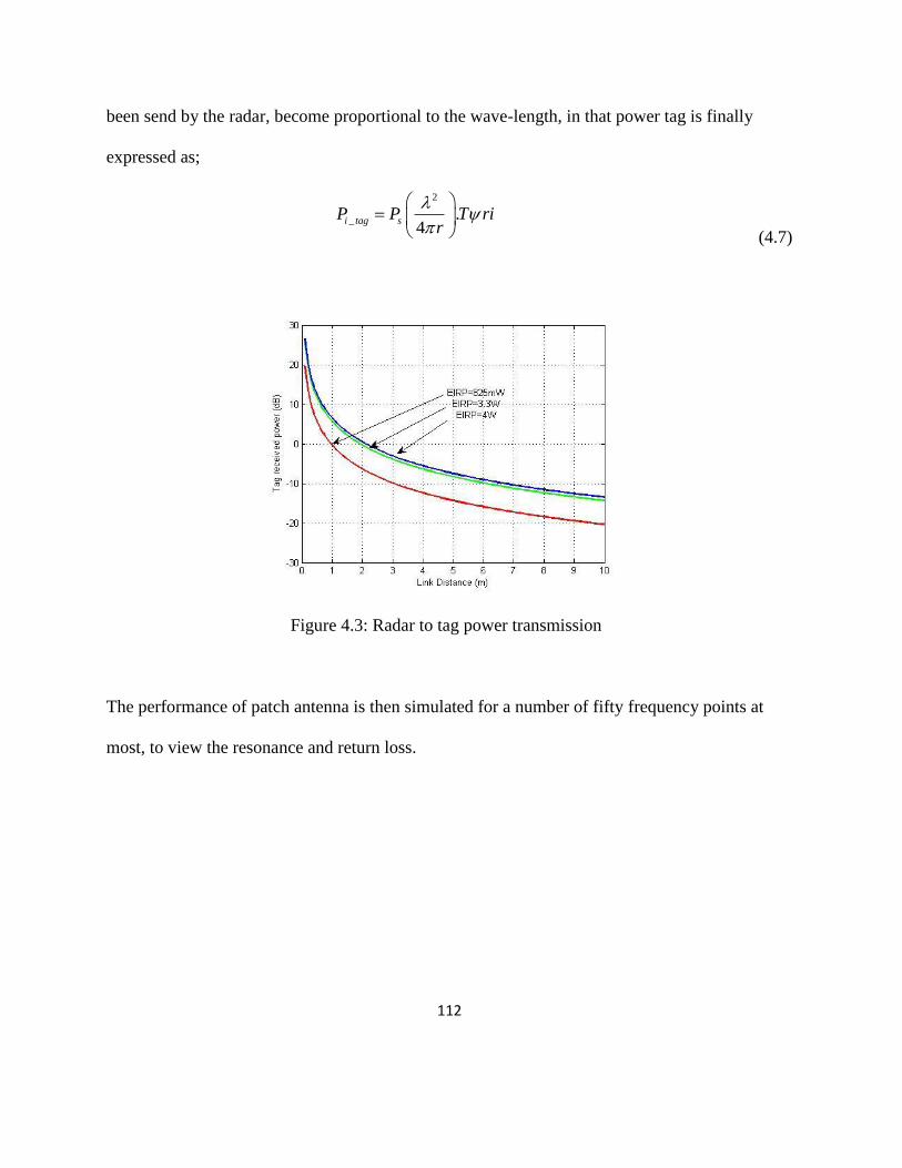
112
been send by the radar, become proportional to the wave-length, in that power tag is finally
expressed as;
2
_ .4
i tag sP P T rir
(4.7)
Figure 4.3: Radar to tag power transmission
The performance of patch antenna is then simulated for a number of fifty frequency points at
most, to view the resonance and return loss.
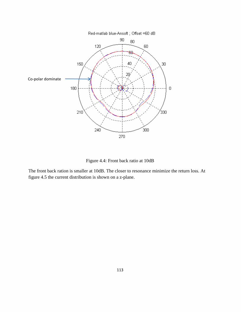
113
Figure 4.4: Front back ratio at 10dB
The front back ration is smaller at 10dB. The closer to resonance minimize the return loss. At
figure 4.5 the current distribution is shown on a z-plane.
Co-polar dominate
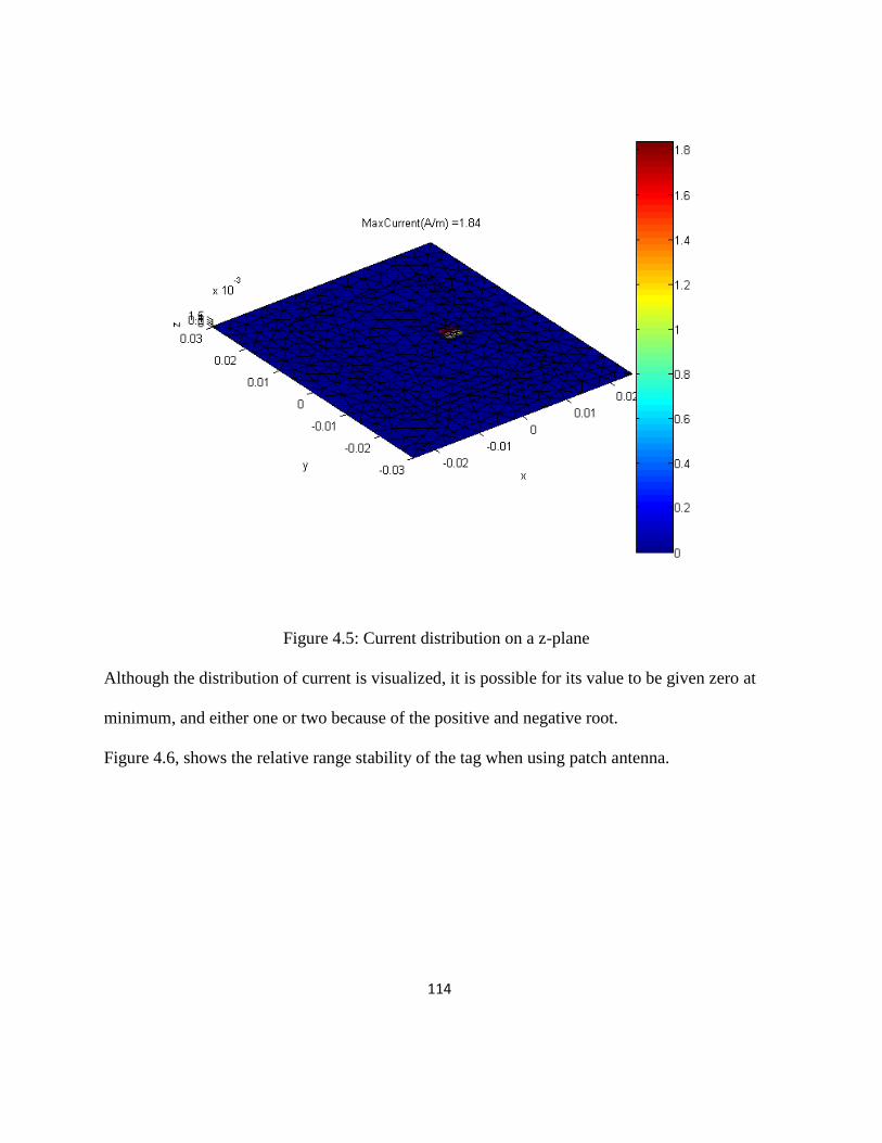
114
Figure 4.5: Current distribution on a z-plane
Although the distribution of current is visualized, it is possible for its value to be given zero at
minimum, and either one or two because of the positive and negative root.
Figure 4.6, shows the relative range stability of the tag when using patch antenna.

115
Figure 4.6: Relative range stability
0 2 4 6 8 10 12 14 16 18 200.25
0.26
0.27
0.28
0.29
0.3
0.31
0.32
0.33
0.34
Radar-range (m)
Measure
ment
err
ors
(m
)
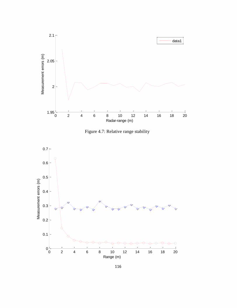
116
Figure 4.7: Relative range stability
0 2 4 6 8 10 12 14 16 18 201.95
2
2.05
2.1
Radar-range (m)
Measure
ment
err
ors
(m
)
data1
0 2 4 6 8 10 12 14 16 18 200
0.1
0.2
0.3
0.4
0.5
0.6
0.7
Range (m)
Measure
ment
err
ors
(m
)
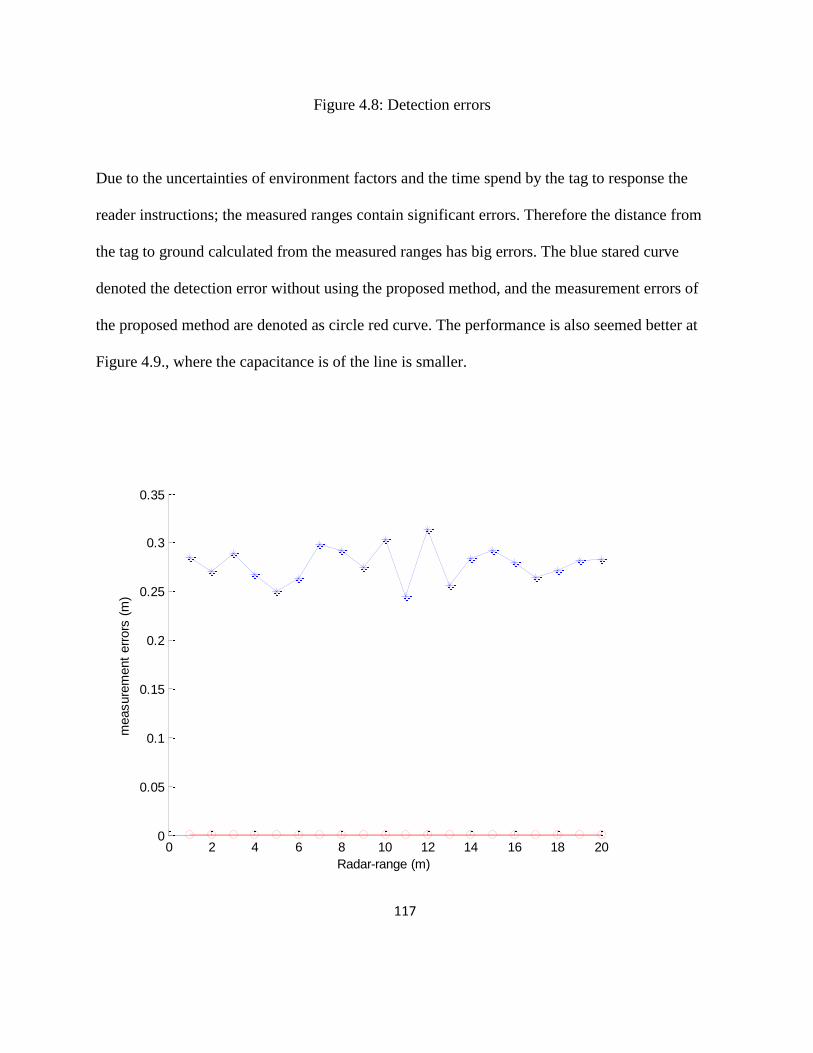
117
Figure 4.8: Detection errors
Due to the uncertainties of environment factors and the time spend by the tag to response the
reader instructions; the measured ranges contain significant errors. Therefore the distance from
the tag to ground calculated from the measured ranges has big errors. The blue stared curve
denoted the detection error without using the proposed method, and the measurement errors of
the proposed method are denoted as circle red curve. The performance is also seemed better at
Figure 4.9., where the capacitance is of the line is smaller.
0 2 4 6 8 10 12 14 16 18 200
0.05
0.1
0.15
0.2
0.25
0.3
0.35
Radar-range (m)
measure
ment
err
ors
(m
)

118
Figure 4.9: Detection errors
Assuming the voltage of the transmission line is varied on Figure 3.3 in chapter 3. The variation
is done by injecting the pulse to the line from 0V to 8KV in simulation. The pulse shape was
chosen because it incorporates three numbers that characterize any pulse.
1.0
0.8
0.6
0.4
0.2
5 10 15
Figure 4.10: Rise time voltage pulse
Rise time
(second)
Voltage (Kv)

119
Figure 4.11: Radar detection errors
0 2 4 6 8 10 12 14 16 18 200
0.1
0.2
0.3
0.4
0.5
0.6
0.7
Radar-range (m)
measure
ment
err
ors
(m
)
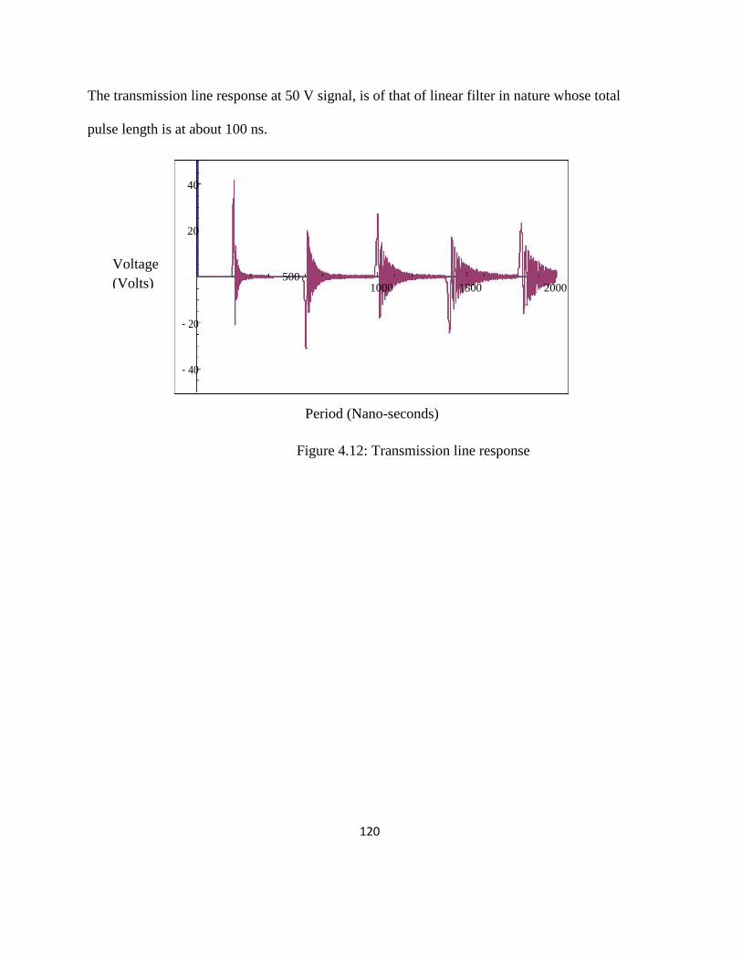
120
The transmission line response at 50 V signal, is of that of linear filter in nature whose total
pulse length is at about 100 ns.
40
20
500 1000 1500 2000
- 20
- 40
Figure 4.12: Transmission line response
Period (Nano-seconds)
Voltage
(Volts)

121
When the pulse voltage is increased to 6KV, the response reveals almost the solid single
outputs seen in Figure 4.10.
6000
4000
2000
500 1000 1500 2000
- 2000
- 4000
- 6000
Figure 4.13: High Voltage injection response
As the same triangulation simulation is done superimposed with the line charge the pulse width
period is now enlarged to 10millisecond and the injection voltage reduced to 50V.
Period (Nano-seconds)
Voltage
(Kv)

122
1.0
0.8
0.6
0.4
0.2
5 10 15 20 25 30
Voltage (V)
Figure 4.14: Increased pulse period
Rise-time (seconds)
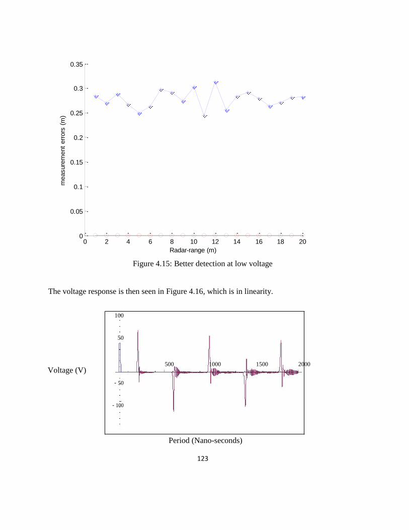
123
Figure 4.15: Better detection at low voltage
The voltage response is then seen in Figure 4.16, which is in linearity.
100
50
500 1000 1500 2000
- 50
- 100
Period (Nano-seconds)
0 2 4 6 8 10 12 14 16 18 200
0.05
0.1
0.15
0.2
0.25
0.3
0.35
Radar-range (m)
measure
ment
err
ors
(m
)
Voltage (V)
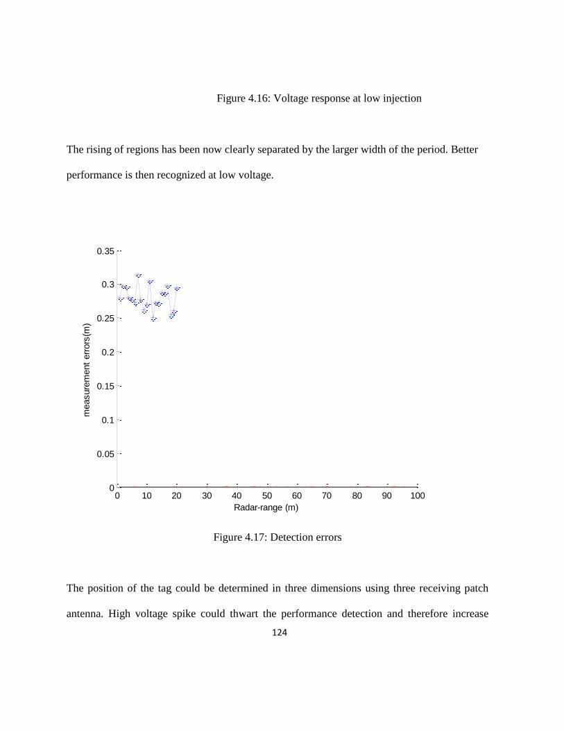
124
Figure 4.16: Voltage response at low injection
The rising of regions has been now clearly separated by the larger width of the period. Better
performance is then recognized at low voltage.
Figure 4.17: Detection errors
The position of the tag could be determined in three dimensions using three receiving patch
antenna. High voltage spike could thwart the performance detection and therefore increase
0 10 20 30 40 50 60 70 80 90 1000
0.05
0.1
0.15
0.2
0.25
0.3
0.35
Radar-range (m)
measure
ment
err
ors
(m)

125
errors. The line quantities such as capacitance, inductance and admittance strengthen the
electric field and therefore play a major role in tag detection.
Detection Error correction attempt using Artificial Neural Network (ANN)
Figure 4.8: ANN error detection correction
The ANN estimator is applied using time lag feed forward network [63]. In this configuration,
p previous readings of x, y and z are used to estimate z. Figure 4.18, depicts the RFID schematic
of the network. A two-weighted layer network consisting of h neurons in the hidden layer and
one output layer is used. The sigmoid function [63] is employed as the activation function of
the hidden neurons but a linear function is applied for the output neurons. The optimum values
x(n-p)
y(n-p)
z(n-p)
x(n)
Input
layer
z
(n)
Hidden
layer
Output
neuron
.
.
y(n)
.
.
z(n)
.
.
.
.
.
.
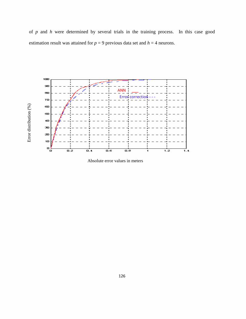
126
of p and h were determined by several trials in the training process. In this case good
estimation result was attained for p = 9 previous data set and h = 4 neurons.
Err
or
dis
trib
uti
on
(%
)
ANN ___
Error correction - - -
Absolute error values in meters

127
Strengths and weaknesses of RFID Sag detection system
Strengths of the method The concept is a more direct method in some ways
as compared to GPS method.
Intermediate calculations or assumptions regarding
ambient weather conditions, conductor
temperature and tension measurements are not
required.
Potentially accurate and cheaper cost
Capable of real time conductor sag detection
The accuracy of the proposed concept is
achievable.
Weaknesses of the method Has not been tested directly on an energized
physical High Voltage (HV) line.
Environmental uncertainties, lack of experience
with the technique, and unstable performance in
HV environment.
Influence to power reflection to tag due to
environment need to be considered.
Table 4.2: Strengths and weakness of RFID

128
CHAPTER 5 DISCUSSION AND CONCLUSION
5.1 Discussion
In employing radio frequency identification for power transmission line conductor sag
measurement different quantities of transmission line and external factors are taken in to
consideration. On metal conductor, the tag sensitivity is better off seen from 8mm than that of a
free space. This gives an additional range by lowering the power of the reader.
The reflection from the surface is not bigger in such that it requires much greater power for the
tag that is close to the surface and at some instance at further distance they do not give
sensitivity that are much better than that which we achieve in free space. The high water content
body or flesh which is close to the tag, impacts the operation of the tag. It is observed that if the
tag was wrapped, sensitivity approaching the free space would be recognized better.
It is seen that paper has a different dielectric constant from that of air meaning that at the
interface between the paper and the air, energy will be lost as it will be reflected away. The
energy would then travel through the paper to the tag. Capacitance of the transmission line as
well as inductance is big internal factors since they cause non linearity and greater electric
charge which affect tag performance.

129
5.2 Conclusion
The results obtained here support the hypothesis in that Radio Frequency Identification system
has a potential of giving an accurate sag measurement in real time. The simulations validate that
the positioning of the tag can be determined in 3D. Although there are some errors, high voltage
varied to a low value to view error change and lastly a neural network was implemented to
decrease the errors identified. With narrow bandwidth which allows RFID not to interfere with
other communication systems, the angle of arrival measurement can virtually be used in
conjunction with range from a single measuring location to determine sag. External and internal
factors which have impact on the performance of the system such as Pole line obstruction or wall
need to be carefully taken into consideration. Although transmission line and radio frequency
identification theories are valid for designing, the system advances need to take place in future to
improve the detection errors on the system.
Corona discharge effect in the transmission lines is a phenomenon in which ionization of the
surrounding air of power conductors take place at voltages greater than critical break down
voltage. When the potential between the power conductors o transmission lines high voltage
lines goes further, increase in hissing noise is experienced which is followed by the violet glow
and the production of ozone gas which finally brings about flash over and electrical break down.
This phenomenon is complex and cannot be easily predicted. Future work will deal with this
phenomenon.

130
Appendix A
List of publications obtained during the research
1. International conference in Electrical Engineering and Technology, (ICEET2013) 22-23 July
2013; Oslo, Norway ISSN 210 376X issued 79 page 1710. Title “Radio Frequency
Identification technology applied on high voltage transmission line for conductor-sag
measurement”
2. International journal of Engineering and Advanced technology (IJEAT) Peer reviewed
ISO-9001:2008 ISSN 2249 – 8958 issue-1, volume-3, page 297-302 New Delhi, India. Title
“Real time Monitoring of High Voltage Power Transmission line: A review of a state-of-the-
art” 25 October 2013
Appendix B
3 D tag-radar positioning code in matlab
function [ x, y ] = two_tri(x1, x2, x3, y1, y2, y3, d1, d2, d3) %2-D tri-function % Inputs: tags 1-3 (x,y) and Distances to Tag % % x_n1 = (d1^2 - d2^2)-(x1^2 - x2^2)-(y1^2 - y2^2)*2*(y3 - y1) % x_n2 = 2*(y2 - y1)*(d1^2 - d3^2) - (x1^2 - x3^2) - (y1^2 - y3^2) % x_d = 2*(x2 - x1)*2*(y3 - y1) - 2*(y2 - y1)*2*(x3-x1) % x = (x_n1 - x_n2)/x_d % y = 2; % x_n11 = (d1^2 - d2^2) - (x1^2 - x2^2) - (y1^2 - y2^2); x_n21 = (d1^2 - d3^2)
- (x1^2 - x3^2) - (y1^2 - y3^2); x_n12 = 2*(y2-y1); x_n22 = 2*(y3-y1);
d11 = 2*(x2-x1); d21 = 2*(x3-x1); d12 = 2*(y2-y1); d22 = 2*(y3-y1);
x_n = [x_n11, x_n12; x_n21, x_n22] d = [d11, d12; d21, d22]
x = x_n/d x = det(x)
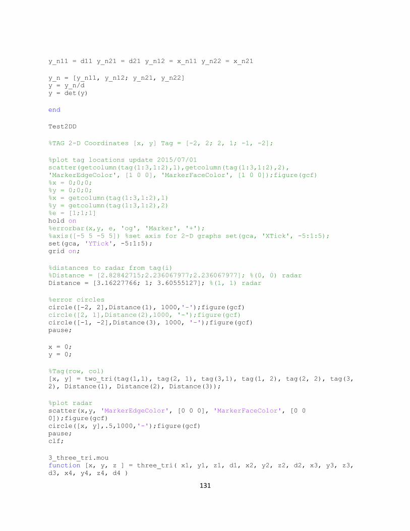
131
y_n11 = d11 y_n21 = d21 y_n12 = x_n11 y_n22 = x_n21
y_n = [y_n11, y_n12; y_n21, y_n22] y = y_n/d y = det(y)
end
Test2DD
%TAG 2-D Coordinates [x, y] Tag = [-2, 2; 2, 1; -1, -2];
%plot tag locations update 2015/07/01
scatter(getcolumn(tag(1:3,1:2),1),getcolumn(tag(1:3,1:2),2),
'MarkerEdgeColor', [1 0 0], 'MarkerFaceColor', [1 0 0]);figure(gcf) %x = 0;0;0; %y = 0;0;0; %x = getcolumn(tag(1:3,1:2),1) %y = getcolumn(tag(1:3,1:2),2) %e = [1;1;1] hold on %errorbar(x,y, e, 'og', 'Marker', '+'); %axis([-5 5 -5 5]) %set axis for 2-D graphs set(gca, 'XTick', -5:1:5); set(gca, 'YTick', -5:1:5); grid on;
%distances to radar from tag(i) %Distance = [2.82842715;2.236067977;2.236067977]; %(0, 0) radar Distance = [3.16227766; 1; 3.60555127]; %(1, 1) radar
%error circles circle([-2, 2],Distance(1), 1000,'-');figure(gcf) circle([2, 1],Distance(2),1000, '-');figure(gcf) circle([-1, -2],Distance(3), 1000, '-');figure(gcf) pause;
x = 0; y = 0;
%Tag(row, col) [x, y] = two_tri(tag(1,1), tag(2, 1), tag(3,1), tag(1, 2), tag(2, 2), tag(3,
2), Distance(1), Distance(2), Distance(3));
%plot radar scatter(x,y, 'MarkerEdgeColor', [0 0 0], 'MarkerFaceColor', [0 0
0]);figure(gcf) circle([x, y],.5,1000,'-');figure(gcf) pause; clf;
3_three_tri.mou function [x, y, z ] = three_tri( x1, y1, z1, d1, x2, y2, z2, d2, x3, y3, z3,
d3, x4, y4, z4, d4 )

132
%3-D tri_tri. 4 anchor nodes % x1 = x coordinate of tag 1 % y1 = y coordinate of tag 1 % z1 = z coordinate of tag 1 % d1 = distance from radar to tag 1
%x_numerator elements x_n11 = (d1^2-d2^2) - (x1^2-x2^2) - (y1^2-y2^2) - (z1^2-z2^2);
%sigma x_n21 = (d1^2-d3^2) - (x1^2-x3^2) - (y1^2-y3^2) - (z1^2-z3^2); %beta x_n31 = (d1^2-d4^2) - (x1^2-x4^2) - (y1^2-y4^2) - (z1^2-z4^2); %phi x_n12 = 2*(y2-y1); x_n22 = 2*(y3-y1); x_n32 = 2*(y4-y1); x_n13 = 2*(z2-z1); x_n23 = 2*(z3-z1); x_n33 = 2*(z4-z1);
%all the individual d11 = 2*(x2-x1); d21 = 2*(x3-x1); d31 = 2*(x4-x1); d12 = 2*(y2-y1); d22 = 2*(y3-y1); d32 = 2*(y4-y1); d13 = 2*(z2-z1); d23 = 2*(z3-z1); d33 = 2*(z4-z1);
%bringing M together into [3, 3] matrix d = [d11, d12, d13; d21, d22, d23; d31, d32, d33];
%bringing numerator together for x x_n = [x_n11, x_n12, x_n13; x_n21, x_n22, x_n23; x_n31, x_n32, x_n33];
%finding x by dividing matrix operation and then determinant x = x_n / d; x = det(x);
%individual y elements y_n11 = 2*(x2-x1); y_n21 = 2*(x3-x1); y_n31 = 2*(x4-
x1); y_n12 = x_n11; %sigma y_n22 = x_n21; %beta y_n32 = x_n31; %phi y_n13 =
2*(z2-z1); y_n23 = 2*(z3-z1); y_n33 = 2*(z4-z1);
%bringing numerator together for y y_n = [y_n11, y_n12, y_n13; y_n21, y_n22, y_n23; y_n31, y_n32, y_n33];
%finding y by dividing matrix operation and then determinant y = y_n / d; y = det(y);
%individual z elements z_n11 = 2*(x2-x1); z_n21 = 2*(x3-x1); z_n31 = 2*(x4-
x1); z_n12 = 2*(y2-y1); z_n22 = 2*(y3-y1); z_n32 = 2*(y4-y1); z_n13 = x_n11;
%sigma z_n23 = x_n21; %beta z_n33 = x_n31; %phi
%bringing z numerator together z_n = [z_n11, z_n12, z_n13; z_n21, z_n22, z_n23; z_n31, z_n32, z_n33];
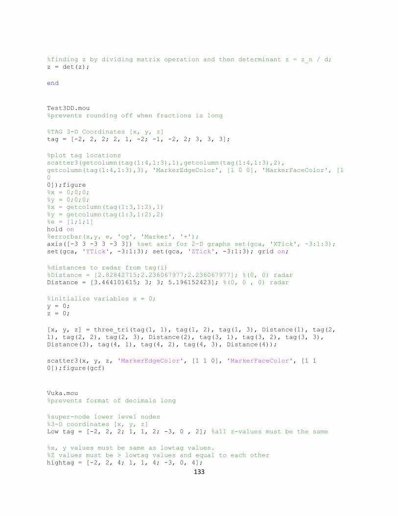
133
%finding z by dividing matrix operation and then determinant z = z_n / d; z = det(z);
end
Test3DD.mou %prevents rounding off when fractions is long
%TAG 3-D Coordinates [x, y, z] tag = [-2, 2, 2; 2, 1, -2; -1, -2, 2; 3, 3, 3];
%plot tag locations
scatter3(getcolumn(tag(1:4,1:3),1),getcolumn(tag(1:4,1:3),2),
getcolumn(tag(1:4,1:3),3), 'MarkerEdgeColor', [1 0 0], 'MarkerFaceColor', [1
0 0]);figure %x = 0;0;0; %y = 0;0;0; %x = getcolumn(tag(1:3,1:2),1) %y = getcolumn(tag(1:3,1:2),2) %e = [1;1;1] hold on %errorbar(x,y, e, 'og', 'Marker', '+'); axis([-3 3 -3 3 -3 3]) %set axis for 2-D graphs set(gca, 'XTick', -3:1:3); set(gca, 'YTick', -3:1:3); set(gca, 'ZTick', -3:1:3); grid on;
%distances to radar from tag(i) %Distance = [2.82842715;2.236067977;2.236067977]; %(0, 0) radar Distance = [3.464101615; 3; 3; 5.196152423]; %(0, 0 , 0) radar
%initialize variables x = 0; y = 0; z = 0;
[x, y, z] = three_tri(tag(1, 1), tag(1, 2), tag(1, 3), Distance(1), tag(2, 1), tag(2, 2), tag(2, 3), Distance(2), tag(3, 1), tag(3, 2), tag(3, 3),
Distance(3), tag(4, 1), tag(4, 2), tag(4, 3), Distance(4));
scatter3(x, y, z, 'MarkerEdgeColor', [1 1 0], 'MarkerFaceColor', [1 1
0]);figure(gcf)
Vuka.mou %prevents format of decimals long
%super-node lower level nodes %3-D coordinates [x, y, z] Low tag = [-2, 2, 2; 1, 1, 2; -3, 0 , 2]; %all z-values must be the same
%x, y values must be same as lowtag values. %Z values must be > lowtag values and equal to each other hightag = [-2, 2, 4; 1, 1, 4; -3, 0, 4];

134
%radar x y z for testing purposes radar = [4; 5; 1];
low_d1 = sqrt((lowtag(1, 1)- radar(1))^2 + (lowtag(1, 2)- radar(2))^2 +
(lowtag(1, 3) - radar(3))^2); low_d2 = sqrt((lowtag(2, 1)- tag(1))^2 + (lowtag(2, 2)- radar(2))^2 +
(lowtag(2, 3)- radar(3))^2); low_d3 = sqrt((lowtag(3, 1)- radar(1))^2 + (lowtag(3, 2)- radar(2))^2 +
(lowtag(3, 3)- radar(3))^2);
%find distances for radar (0, 0, 0) high_d1 = sqrt((hightag(1,1)- radar(1))^2 + (hightag(1, 2)- radar(2))^2 +
(hightag(1, 3)- radar(3))^2); high_d2 = sqrt((hightag(2,1)- radar(1))^2 + (hightag(2, 2)- radar(2))^2 +
(hightag(2, 3)- radar(3))^2); STOPPED 07/07/15 high_d3 = sqrt((hightag(3,1)- radar(1))^2 + (hightag(3, 2)- radar(2))^2 +
(hightag(3, 3)- tag(3))^2);
lowDistances = [low_d1; low_d2; low_d3]; highDistances = [high_d1; high_d2; high_d3];
%height of radar z = callHeight(lowtag, hightag, lowDistances, highDistances) %array for 2-D trilateration distances = [0; 0; 0]; distances = findDistance(lowtag, hightag, lowDistances, highDistances);
[x, y] = two_tri(lowtag(1, 1), lowtag(2, 1), lowtag(3, 1), lowtag(1, 2),
lowtag(2, 2), lowtag(3, 2), distances(1), distances(2), distances(3))
Vuka_height.mou function [ radarHeight ] = callHeight(lowtag, hightag, lowDistances,
highDistances) %VukaHEIGHT Find height of tag % Using supernode distances, use trig to determine height of tag
heightDifference = hightag(1, 3) - lowtag(1, 3);
height = [0; 0; 0];
height(i) = hightag(i, 3) - ((highDistances(i)^2 - lowDistances(i)^2 + heightDifference^2)/(2*heightDifference)); end
%set x = 0 for below x = 0; %find average height found by the 3 super-nodes for more accurate results for
i = 1:3 x = x + height(i); end
135
List of references
1. Glorver, B. & Bhatt, H. (2003) RFID Essentials. Research trends in radio frequency
identification technology, 7(1), 22-25.
2. A. Cataliotti et al., “Characterization of current transformers in the presence of harmonic
distortion, Presented at the” IEEE Int. Instrum. Meas. Technol. Conf., Victoria, Vancouver
Island, Canada, 2008.
3. L. Fish, “Low Cost Sensors for Real Time Monitoring of Overhead Transmission Lines”.
Washington, DC: Underground Systems Inc., 2006.
4. February 5, 2010, Tension Monitor [online], available online http://www.cat-1.com)
5. G. Thomas Heydt, fellow, IEEE, “Application of the Global Positioning System to the
Measurement of overhead Power Transmission Conductor Sag,” IEEE Trans. Power Del., Vol.
17 NO. 1, pp 273-278, January 2002.
6. A. Edelstein, “Advances in magnetometry,” J.Phys., Cond. Matter, vol. 19, pp. 165-217, Apr.
2007.
7. R.G. Olsen and K.S. Edward, “A new method for real-time monitoring of high-voltage
transmission-line conductor sag,” IEEE Trans, Power Del., vol.17 no.4 pp. 1142-1152, Oct.
2002.
8. C Mensah-Bonsu, “Novel application of Magnetoresisteve Sensors for High-Voltage
Transmission-Line Monitoring,” IEEE on Magnetics, Vol. 47 NO. 10 October 2011.
9. G. Ramon, IEEE Task Force Chairman, “Dynamic thermal line rating summary and status of the
state-of-the-art technology,” IEEE Trans. Power Delivery, vol. PWRD-2, pp. 851-856, July
1987.
136
10. S.W. Rienstra, “Nonlinear free vibration of coupled spans of overhead transmission lines,” in
proc. 3rd
Eur. Conf. Math. Ind., 1988 pp 133-134.
11. R. G. Olsen and K.S. Edwards, “A new method for real-time monitoring of high voltage
transmission line conductor sag,” IEEE Trans. Power Del., vol.17, no. 4pp 1142 – 1152, Oct.
2002.
12. Wernich de Villiers, and Arthur Burger, “Real-time sag monitoring system for high voltage
transmission lines based on power-line carrier signal behavious” IEEE Trans. On power del.,
Vol.23, NO.1, January 2008.
13. Xignlong Zhu, and JipingShou, “An Autonomous Obstacles Negotiating Inspection Robot for
Extra-High Voltage Power Transmission lines”.
14. Hectro Beltran San Sequndo, and Vicente Fuster, “Automated Inspection of Electric
Transmission line: The power supply system”
15. Graham Hall “maxwell’s electromagnetic theory and special relativity” Phil. Trans. R. Soc. A
2008, published 28 May 2008.
16. Y.H Gu, and S Berlinjn, “Practical applications of automatic image analysis for overhead lines”
22nd
Int. Conf. on Electricity distribution, Stockholm, Norway 10-13 June 2013.
17. A Martin and S Tosunoglu, “image processing technique for machine vision” univ. of florida.
18. MJ Tunstal et al., “State of the art of conductor galloping, 2002”
19. T.S Hlalele & S Du “Application of a Radio Frequency Identification Technology on High
voltage Transmission Line for conductor sag measurement” ICEET2013 Conf. Proceedings,
Norway 22-23 July 2013.
20. IEEE Std 1159-2009 IEEE Recommended Practice for Monitoring Electric Power Quality
21. DA Douglass & Ridley Trash “Sag and Tension of conductor” 2013

137
22. R.G. Olsen and K.S. Edwards, “A new method for real-time monitoring of high voltage
transmission line conductor sag,” IEEE Trans. Power Del., vol.17, no. 4 pp 1142 – 1152, Oct.
2002.
23. Kern. C (1999), “ RFID technology – recent development and future requirements”, proceedings
of the European Conference on Circuit Theory and Design ECCTD99, Stresa, vol.1 pp. 25-81,
available at www.x.ident.com/pdf/develpment rfid.pdf.
24. 2006 MIT, American institute of Aeronautics’ and Astronautics Scientists, MA 02139 USA
white paper IEEE 2006.
25. Information Technology Association of America (ITAA), “Radio Frequency Identification:
RFID coming of Age,” White Paper, information Technology Association of America,
Arlington, VA, June 2004. Available online: http:/www.itaa.org/rfid/docs/rfid.pdf.
26. SCIS 2007. The 2007 Symposium on Cryptography and information security sasebo, Japan, Jan
23 – 26, 2007 (The Electronics, information and communication Engineers).
27. K. Findenzeller, RFID Handbook: Fundamentals and Applications in Contac less smart cards and
identification, New York: John Wiley and Sons, 2003.
28. S. M. Amin and B.F. Wollenberg, “Toward a smart grid: Power delivery for the 21st century,”
IEEE Power Energy Mag., vol. 3 no. 5, pp.34-41, Sep. 2002
29. A Polycarpou, “Power Quality and Voltage Sag Indices in Electrical Power systems” Frederick
University Cyprus, 2005 pp140-155.
30. M Bouc, D Simpiont and I Stojmenovic, “RFID Systems research trends and challenges” 2010
John Wiley & Sons Ltd., pp 57-90

138
31. Charles Mutigwe&FarhadAghdasi, “Research Trends in RFID Technology”, Presented at the
Central University of Technology, Free State. Annual Engineering seminar, Bloemfontein, 2008.
32. Marrocco, G. (2008) “The art of UHF RFID antenna design: impedance-matching and size-
reduction techniques”, IEEE Antennas and Propagation Magazine, 50(1): 66-79.
33. Bridgelall, R. (1999) UHF Tags – the answer to the ratail supply chanin’sprayres? RF
Innovations Magazine August.
34. Bridgelall, R (2002) Bluetooth/802.11 protocol adaptation for RFID tags, Proceedings of the 4th
European Wireless Conference, Feb. 28.
35. Mandal. S and Sarpeshkar, R. (2007) Low-power CMOS rectifier design for RFID applications,
IEEE Transactions on Circuits and Sstems, 54(6): 1177-1188
36. AA Smith,Jr, (1998) Radio Frequency Principles and Applications. New York: IEEE Press
37. P.R Gray, P.J Hurst, S.H Lewis, and R.G Meyer, (2001) Analysis and Design of Analog
Integrated Circuits, 4th
edn. New York: John Wiley & Sons, Ltd, pp. 127 – 128.
38. J. Misic , 2009 Recommended Wireless Network standard:IEEE 802.11b and IEEE 802.15.4.
39. B.Skalar, (1988) Digital Communications Fundamentals and Applications’. New jersey: Prentice
Hall
40. EPC global Inc. (2005) Radio Frequency Identification, protocols Class-1 Generation-2 UHF
RFID
41. U. Karthaus and M. Fischer (2003) “fully integrated passive UHF RFID transponder IC with
16.7-micro-Watt”.
42. Admirat, P., M. Maccagnan, and B. De Goncourt, 1988 ‘Influence of Joule effect and of climatic
conditions on liquid water content of snow accreted on conductors’ Proc. Of the 4th
International
Workshop on Atmospheric Icing of Structures, Paris.

139
43. Chadha, J 1974b. ‘A dynamic Model Investigation of Conductor Galloping’ IEEE Winter power
Meeting. Paper 74 59-2
44. Anjo, K., S. Yamasaki, Y. Matsubayshi, Y. Nakayama, A. Otsuki, and T. Fujimura. 1974. An
Experimental Study of Bundle Galloping on the kasatory Yama Test lin for Bulk power
Transmission. CIGRE report 22-04. Paris.
45. Bleviens, R.D 1990. ‘Flow Induced Vibration. ‘Van Nostrand Reinhold. New York. Second
Edition.
46. Fujii,Y.,T.KoyamaandT.Sawamoto.1997.“Counter measures against Conductor
Galloping.”Paper11.Colloquium on Environmental Impact of OHL inJapan.CIGRESC22.Sendai
Meeting.
47. Gartshore,I.S. 1973. “The effects of free stream turbulence on the drag of rectangular two-
dimensional prisms. “Boundary Layer Wind Tunnel Laboratory 4-73, University of Western
Ontario.
48. Gurung, C.B., H.YamaguchiandT.Yukino.2002.“Identification of large amplitude wind-induced
vibration of ice- accreted transmission lines base on field observed data” Engineering
Structures,24,pp. 179-188.
49. Gurung, C.B., H.Yamaguchi, andT.Yukino.2003. “Identification and Characterization of
Galloping of Tauranga Test Line Based on Multi-channel Modal Analysis of Field Data.
Journal of Wind Engineering & Industrial Aerodynamics. Vol. 91, Issue7.June. Pp. 903-924.
50. Halsan, K.A., D.G. Havard, S. M. Fikke, andA. Gerezgiher. 1998. “Galloping Studies at
Statnett Using Remote Monitoring.”CIGRESC22,WG11meeting.Graz, Austria. Paper No.22-
98.
51. Harvard, D.G.1978. “Status of Conductor Galloping Research at Ontario Hydro. “Second

140
Canadian Workshop on Wind Engineering. IREQ Varennes, Quebec. September 28-29.
52. Harvard, D.G. and J.C. Pohlman.1979. “Field Testing of Detuning Pendulums for Controlling
Galloping of Single and Bundle Conductors.” Paper A79499-5.IEEESymposium on Mechanical
Oscillations of Overhead Transmission Lines. Vancouver, Canada. July.
53. Harvard, D.G.1979a. “Detuning for Controlling Galloping of Single Conductor Transmission
Lines.”PaperA79500-0. IEEE Symposium on Mechanical Oscillations of Overhead
Transmission Lines. Vancouver, Canada July.
54. Havard,D.G.1979b.“DetuningPendulumsforControllingGallopingofBundleConductorTransmissi
onLines.”Paper79 501-8. IEEE Symposium on Mechanical Oscillations of Overhead
Transmission Lines. Vancouver, Canada. July.
55. Harvard, D.G.1979c.Galloping Control by Detuning. EPRI Research ProgramRP-1095.Progress
Report No.2.Ontario
56. Havard,D.G.andJ C. Pohlman. 1981. “The Economics of Galloping Control.” CEA
International Symposium on overhead conductor dynamics. Toronto
57. Harvard, D.G. and J.C.Pohlman.1984.“FiveYears’Field Trials of Detuning Pendulums for
Galloping Control.” IEEE Transactions on Power Apparatus and Systems. Vol. PAS-103,No
2.pp.318-327.February.
58. Havard,D.G. and C.J.Pon.1990. “Use of Detuning Pendulums for Control of Galloping of Single
Conductor and Two- and Four-Conductor Bundle Lines.” Fifth International Workshop on
Atmospheric Icing of Structures. Tokyo.
59. Harvard,D.G.1996.“FifteenYears Field Trials of Galloping Controls for Overhead Power
Lines.”IWAIS’95.7th
international workshop on atmospheric Icing of structures. Chicoutimi,
Canada. June 3-6
141
60. Harvard, D.G.1997.“Analysis of Field Data on Galloping of Single and Bundle Conductors with
and without Control Devices.” Paper16, International Seminar on Cable Dynamics. Tokyo.
October 1997.
61. Hillier,R. and R.J.Cherry. 1981. “The effect of stream turbulence on separation bubbles.
“Journal of Wind Engineering and Industrial Aerodynamics, v. 8,pp. 49-58.
62. Hoerner,S.F. 1965.“Fluid dynamic drag,” published by the author,
New York, pp. 415.
63. M. A. El-Sharkawi, D. Niebur, 1996 “A Tutorial Course on
Artificial Neural Networks with Applications to Power systems”,
IEEE Power Engineering Society, IEEE Catalogue Number: TP
112-0, New York.


![Radio Frequency Identification [JePartage]](https://img.dokumen.tips/doc/110x75/5a6533127f8b9a5b558b521d/radio-frequency-identification-jepartage.jpg)