Embed Size (px)
Citation preview
Model-Based Robust Control Design for
Magnetostrictive Transducers Operating
in Hysteretic and Nonlinear Regimes
James M. Nealis1 and Ralph C. Smith2
Department of MathematicsCenter for Research in Scientific Computation
North Carolina State UniversityRaleigh, NC 27695
Abstract
This paper addresses the development of robust control designs for high performance smart material trans-ducers operating in nonlinear and hysteretic regimes. While developed in the context of a magnetostrictivetransducer used for high speed, high accuracy milling, the resulting model-based control techniques can bedirectly extended to systems utilizing piezoceramic or shape memory alloy compounds due to the unifiednature of models used to quantify hysteresis and nonlinearities inherent to all of these materials. Whendeveloping models and corresponding inverse filters or compensators, significant emphasis is placed on theutilization of the material’s physics to provide the accuracy and efficiency required for real-time implementa-tion of resulting model-based control designs. In the material models, this is achieved by combining energyanalysis with stochastic homogenization techniques whereas the efficiency of forward algorithms is combinedwith monotonicity properties of the material behavior to provide highly efficient inverse algorithms. Theseinverse filters are then incorporated in H2 and H∞ theory to provide robust control algorithms capable ofproviding high accuracy tracking even though the actuators are operating in nonlinear and hysteretic regimes.Through numerical examples, it is illustrated that the robust designs incorporating inverse compensators canachieve the required tracking tolerance of 1-2 µm for the motivating milling application whereas robust designswhich treat the uncompensated hysteresis and nonlinearities as unmodeled disturbances cannot achieve designspecifications.
Keywords: Robust control design, hysteresis, constitutive nonlinearities, inverse filter, magnetostrictivetransducers
1Email: [email protected], Telephone: (919) 515-89682Email: [email protected]; Telephone: (919) 515-7552; Corresponding Author
i

1 Introduction
A growing emphasis in advanced control system designs focuses on the use of multifunctional materials, suchas piezoceramics, magnetostrictives, and shape memory alloys, in integrated transducers to improve controlauthority and performance, reduce weight, and minimize power requirements. For example, piezoceramiccompounds have both actuator and sensor capabilities due to the direct and converse piezoelectric effects,microscale set point accuracy, and high frequency (kHz) operating capabilities. This has led to their use inapplications ranging from nanopositioning mechanisms in an atomic force microscope (AFM) [23, 24, 25, 26]to inertial sensors in an accelerometer [9]. Magnetostrictive materials also offer both actuator and sensorcapabilities as well as broadband transduction and large output forces. Recent applications and productsexploiting these properties include high accuracy, high speed milling devices [29, 38] and torque sensing forsteering systems [5, 22]. Shape memory alloys (SMA) operate at lower frequencies (< 100 Hz for bulk materials)but offer the largest power densities of the three compounds. Hence they are being considered for applicationsranging from vibration dissipation in buildings and flexible aerospace structures to active shape configurationof an airfoil to optimize flight characteristics while minimizing drag [19, 27].
Whereas all of these compounds offer significant and unique actuator and/or sensor capabilities, they alsoexhibit varying degrees of hysteresis and constitutive nonlinearities throughout their operating range andfrequency, stress and temperature-dependencies in various drive regimes. In some cases, the hysteresis canbe mitigated through the drive electronics – e.g., charge or current control for piezoceramics is appropriatein certain applications [15, 16, 17] – or feedback loops in the transducer. However, noise-to-signal ratios insensor data and diminishing characteristics of high pass filters precludes a sole reliance on feedback loops forbroadband and high frequency transduction. Furthermore, because damping properties of the materials areproportional to the area of the hysteresis loop, it is often advantageous to maximize rather than minimize hys-teresis in the transducer design. This necessitates the development of robust control designs which incorporatethe hysteresis in a manner which achieves specified tracking, damping and general performance criteria whileemploying the transducer materials in the nonlinear regimes which provide them with their unique actuatorand/or sensor capabilities.
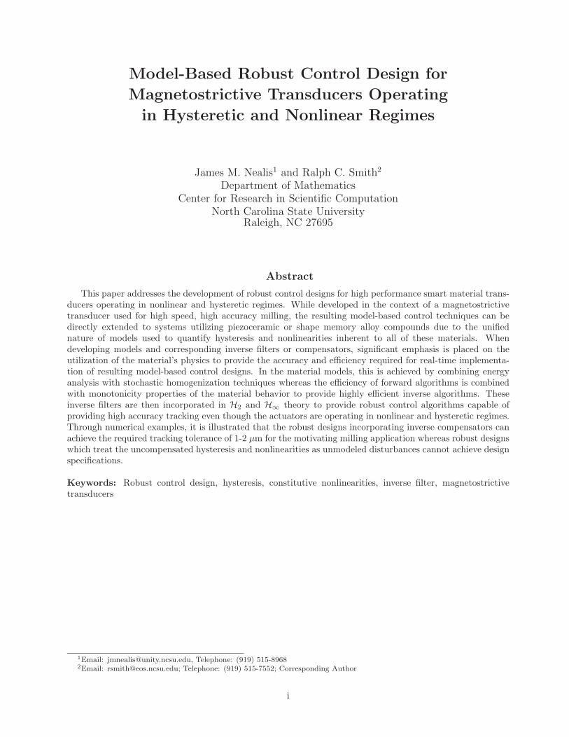
In this paper, we develop a model-based robust control design in the context of a magnetostrictive trans-ducer operating in nonlinear and hysteretic regimes with high accuracy, high speed tracking specifications.A motivating application entails the use of the magnetostrictive transducer to mill out-of-round automotiveparts at speeds of 3000 rpm and tracking tolerances of 1-2 µm as detailed in [29, 38] and depicted in Figure1a. During the milling process, the cutting tip starts from a position of rest, is moved adjacent to the ma-terial, and then must follow a prescribed periodic trajectory required to yield the final geometry. Hence thetrajectory to be tracked has the form depicted in Figure 1b. The forces required to drive the cutting head aregenerated through the reorientation of magnetic moments in the Terfenol-D rod in response to a field H(t)produced by a current I(t) to the surrounding solenoid. The surrounding magnet provides the bias necessaryto achieve bidirectional strains. As illustrated in Figure 2, the field-magnetization and field-strain relationsfor the transducer exhibit significant hysteresis and constitutive nonlinearities which must be accommodatedin models and model-based control designs.
Both the material behavior and control issues associated with this application are representative of thoseencounted when alternatively considering piezoceramic or shape memory alloy transducers and hence this
(b)
0
Time
Milled Object
(a)
Pos
ition
CuttingHead
����������
����������
��������
��������
��������
SpringWasher
Compression Bolt Terfenol−D Rod
Wound Wire Solenoid Permanent Magnet
Figure 1: (a) Prototypical magnetostrictive transducer used for high speed, high accuracy milling. (b) Tra-jectory to be tracked by the cutting head.
1
−1 −0.5 0 0.5 1
x 105
−6
−4
−2
0
2
4
6x 10
5
Field (A/m)
Mag
netiz
atio
n (A
/m)
−1.5 −1 −0.5 0 0.5 1 1.5
x 105
0
0.2
0.4
0.6
0.8
1
1.2
1.4x 10
−3
Field (A/m)
Str
ain
(a) (b)
Figure 2: Hysteretic data measured in a Terfenol-D transducer as reported in [6]: (a) field-magnetizationrelation, and (b) field-strain relation.
transducer provides a framework for addressing robust control design for a broad range of multifunctionalmaterials while clarifying the development by focusing on a specific application. It is detailed in [33, 35, 36]that the common domain and ferroic nature of ferroelectric, ferromagnetic and ferroelastic materials can beexploited to develop unified models for the compounds and we employ one such model in the robust controldesign developed here. Hence the material behavior shown in Figure 2 is representative of that exhibitedby a broad range of compounds and is characterized by unified models appropriate for all of these materials.Furthermore, the high accuracy specifications for the motivating milling application are representative of thoseencountered in a range of smart material control applications.
From the perspective of control design, the hysteresis inherent to the compounds introduces phase delayswhereas saturation behavior introduces additional nonlinearities. These combined nonlinear effects producedisturbances which, if left unattenuated, produce unacceptable degradation in tracking performance. Sensornoise also produces disturbances which degrade the efficacy of state estimates and subsequent control inputs.We address both effects when constructing robust control designs for magnetostrictive transducers.
One strategy for designing robust control laws for hysteretic actuators is to employ nonlinear constitutivemodels to characterize the disturbances or perturbations d which must be accommodated by control designs.This can reduce overly conservative robustness margins constructed solely through characterization experi-ments. A second strategy is to employ the models to construct inverse representations or compensators whichcan be employed as filters before the hysteretic actuator in the manner depicted in Figure 3. While suchcompensation is never exact due to discretization and modeling errors, the mismatch between inverse andhysteretic device can be designed to be small thus significantly reducing the disturbance d associated with thetransducer. It is this latter strategy that we consider here.
The use of model-based inverse representations for piezoceramic, magnetostrictive and shape memory com-pounds is not new and has received substantial attention in the context of adaptive, classical, and optimal
u+du P
Figure 3: Approximate model inverse employed as a filter for robust control design in hysteretic and nonlinearsystems.
2

(LQR) control designs [3, 4, 10, 11, 21, 28, 39, 40]. The primary emphasis has focused on Preisach represen-tations (e.g., see [39, 40]), due to their rigorous mathematical foundation and invertibility, as well as domainmodels [21, 28]. While both modeling frameworks can be unified to quantify hysteresis in general ferroic com-pounds, both suffer disadvantages which degrade subsequent control performance in a number of applications.The Preisach methodology must be extended to accommodate the noncongruency, temperature-dependentand reversible behavior exhibited by magnetic (and most ferroic) materials whereas the domain-based theoryof [13, 18, 32, 34] requires extensive modifications to guarantee the closure of minor loops in state feedbackregimes. Furthermore, there is a growing emphasis on the design of control algorithms which accommodatestrongly transient and quickly changing dynamics and are robust with respect to a variety of disturbances.This motivates the development of robust control designs utilizing inverse representations based on the mod-eling framework developed in [30, 31] for ferromagnetic materials with analogous models for piezoceramiccompounds [37], shape memory alloys [19, 27], and unified ferroic compounds [35, 36].
We consider both H2 and H∞ designs since the disturbances can be interpreted in a variety of manners.Since the H2 norm quantifies the maximum amplitude in the output due to bounded energy inputs, it pro-vides a natural measure for sensor noise as well as disturbances due to both approximately compensated oruncompensated hysteresis. The variability due to uncompensated or partially compensated hysteresis and con-stitutive nonlinearities can also be viewed as a structural uncertainty in the actuator model which motivatesconsideration of the H∞ norm.
The emphasis in this paper focuses on the incorporation of physics through energy-based techniques toprovide control designs capable of achieving stringent tracking and speed criteria using advanced transducerdesigns rather than the analytical development of new control theories. Secondly, we emphasize the develop-ment of model-based control designs having the capability for real-time implementation at the speeds dictatedby eventual applications. We rely on previous H2 and H∞ theory – e.g., see [1, 8, 20, 41, 42] – to providea baseline for comparison in the absence of inverse compensation and a starting point from which to initiaterobust control designs that incorporate the physical mechanisms which produce hysteresis through inversecompensators.
In Section 2, we summarize the development of nonlinear constitutive relations which quantify the inherenthysteresis, an algorithm for constructing inverse relations, and the system models used to characterize themagnetostrictive transducer depicted in Figure 1. We provide a system representation in Section 3 along withappropriate weighting filters and the H2 and H∞ theory used to construct robust control algorithms. Weillustrate the performance of these designs through numerical examples in Section 4. Specifically, we illustratethat for physically reasonable disturbance levels, designs based solely on H2 or H∞ algorithms do not achievespecified control criteria whereas inclusion of the model-based inverse filters improves performance to the pointwhere tracking criteria are achieved.
2 Transducer Model
The key to constructing an inverse compensator which accommodates hysteresis and constitutive nonlinearitiesis the development of material models which can be efficiently inverted. In this section, we consider the con-struction of models which quantify magnetostrictive transducer properties in two steps: (i) the construction ofconstitutive models which incorporate inherent hysteresis and material nonlinearities, and (ii) the employmentof these constitutive models to quantify transducer outputs due to specified current inputs. This provides aframework for developing the model inverses employed in the robust control design in Section 3.
2.1 Nonlinear Constitutive Relations
The magnetic and magnetomechanical constitutive models we employ are based on the theory developedin [30, 31] and we summarize here those aspects relevant to the construction of magnetostrictive transducermodels. For this discussion, we make the assumptions that temperatures are fixed, that eddy current losses areminimal and that prestress levels are sufficiently large that stress anisotropies dominate crystalline anisotropies.The assumption of fixed temperature is valid for magnetostrictive transducers utilizing water cooling whereaslow frequency operating regimes or laminated rod designs reduce eddy current losses. Finally, the prestresslevels which optimize performance are typically sufficient to dominate crystalline anisotropies [2] so the finalassumption is valid for present transducer designs.
3
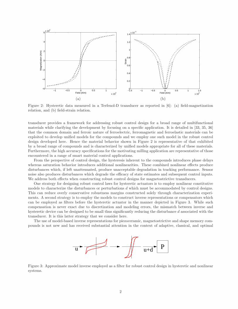
To construct appropriate Helmholtz and Gibbs energy relations, we consider first the case in which appliedstresses are either absent or negligible. Under the assumption that dipoles orient either with the applied fieldor diametrically opposite to it, which is valid for operating regimes in which stress anisotropies dominatecrystalline anisotropies, and fixed temperature regimes, it is illustrated in [31] that a reasonable form of theHelmholtz energy is
ψ(M) =
12η(M + MR)2 , M ≤ −MI
12η(M −MR)2 , M ≥ MI
12η(MI −MR)
(M2
MI−MR
), |M | < MI .
(1)
As depicted in Figure 4, MR and MI respectively denote the point at which the minimum of ψ occurs andthe inflection point. The point MR is also the local remanence magnetization at the domain level. Finally,the fact that η is the reciprocal of the slope in the H-M relation after switching can be utilized to determineinitial parameter values when establishing the model for a given piezoceramic compound and application.
In the absence of applied stresses σ, a suitable magnetic Gibbs energy relation, which incorporates thework due to an applied field H, is
G = ψ −HM. (2)
Note that the magnetostatic energy is E = µ0HM where µ0 denotes the magnetic permeability. The Gibbsrelation (2) can thus be interpreted as incorporating µ0 into ψ for simplicity.
To incorporate magnetoelastic coupling, we employ the extended Helmholtz relation
ψe(M, ε) = ψ(M) +12Y Mε2 − Y MζεM2 (3)
and corresponding Gibbs energy
G(H,M, ε) = ψ(M) +12Y Mε2 − Y MζεM2 −HM − σε (4)
where ψ is specified by (1) and ε denotes longitudinal strains in the material. Here Y M denotes the Young’smodulus at constant magnetization and ζ is a magnetoelastic coupling coefficient. We note that the secondterm in (3) incorporates the elastic energy. The quadratic dependence on the magnetization is motivatedby characterization experiments [7] and can be theoretically justified in magnetostrictive transducers sinceprestress levels are such that stress anisotropies dominate crystalline anisotropies so that strains are dueprimarily to quadratic rotation processes.
G 2 (H ,M)1G (HG(M)= (0,M)
c
RI
I
R
0
,M)ψ
(b)
(a)
H
M M MM M
M
H
MM
M
M
M
HH
Figure 4: (a) Helmholtz energy ψ and Gibbs energy G for σ = 0 and increasing fields H. (b) Dependence ofthe local magnetization M on the field H at the lattice level in the presence of thermal activation.
4

Local average relations for the mesoscale magnetization are derived for two operating regimes: (i) condi-tions for which thermally activated relaxation processes are significant and, (ii) regimes for which relaxationprocesses are negligible. To incorporate relaxation processes, the Gibbs energy G is balanced with the relativethermal energy kT/V over a lattice volume V through the Boltzmann relation
µ(G) = Ce−GV/kT (5)
which quantifies the probability µ of achieving the energy level G. Here C denotes a constant of integrationwhich is constructed to have a value of unity when integrated over all admissible moment orientations, kdenotes Boltzmann’s constant, and T is the fixed temperature of operation. Under the assumption of twomoment orientations, the local average magnetization is given by
M = x+〈M+〉+ x−〈M−〉 (6)
where x+ and x− respectively denote the fraction of moments having positive and negative orientations and
〈M+〉 =
∫∞MI
Me−G(H,M)V/kT dM∫∞MI
e−G(H,M)V/kT dM, 〈M−〉 =
∫ −MI
−∞ Me−G(H,M)V/kT dM∫ −MI
−∞ e−G(H,M)V/kT dM
are the expected magnetization values due to positively and negative oriented moments. The moment fractionssatisfy the evolution equations
x+ = −p+−x+ + p−+x−x− = −p−+x− + p+−x+
where
p+− =
√kT
2πm
e−G(H,MI)V/kT∫∞MI
e−G(H,M)V/kT dM, p−+ =
√kT
2πm
e−G(H,−MI)V/kT∫ −MI
−∞ e−G(H,M)V/kT dM
are the likelihoods of switching from positive to negative orientations and conversely. Here m is the mass oflattice volume V . As depicted in Figure 4, the relation between the applied field H and the local averagemagnetization M exhibits both hysteresis and nonlinear transition because the local magnetization (6) isprobabilistic. The steepness of the transition depends on the ratio of G to kT/V .
For operating regimes in which thermally activated relaxation processes are negligible, the relative thermalenergy kT/V can be ignored and local average magnetization values M are computed directly from thenecessary condition ∂G
∂M = 0, or equivalently H = ∂ψe
∂M . This yields the linear relation
M =H
η − 2Y Mζε+ ∆
MRη
η − 2Y Mζε(7)
which illustrates that η denotes the reciprocal slope after switching in the absence of strains, MR is a localremanence value as depicted in Figure 4, and ∆ indicates the moment orientations. To specify ∆ and henceM , we employ the Preisach notation
[M(H, ε;Hc, ξ)](t) =
[M(H, ε;Hc, ξ)](0) , τ(t) = ∅
Hη−2Y M ζε
− MRηη−2Y M ζε
, τ(t) 6= ∅ and H(max τ(t)) = −Hc
Hη−2Y M ζε
+ MRηη−2Y M ζε
, τ(t) 6= ∅ and H(max τ(t)) = Hc
(8)
where Hc = η(MR −MI), the transition times are specified by
τ(t) = {t ∈ (0, Tf ] | H(t) = −Hc or H(t) = Hc}and the initial moment orientation is
[M(H, ε;Hc, ξ)](0) =
H
η−2Y M ζε− MRη
η−2Y M ζε, H(0) ≤ −Hc
ξ , −Hc < H(0) < Hc
Hη−2Y M ζε
+ MRηη−2Y M ζε
, H(0) ≥ Hc .
Here ξ denotes the initial magnetization of the points with field levels between −Hc and Hc.
5
H H
M
HRM
M cI
M
M M
G G
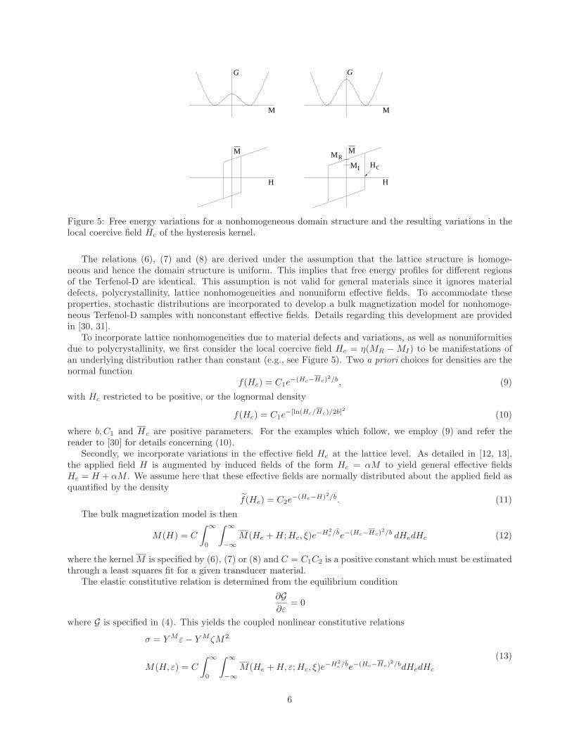
Figure 5: Free energy variations for a nonhomogeneous domain structure and the resulting variations in thelocal coercive field Hc of the hysteresis kernel.
The relations (6), (7) and (8) are derived under the assumption that the lattice structure is homoge-neous and hence the domain structure is uniform. This implies that free energy profiles for different regionsof the Terfenol-D are identical. This assumption is not valid for general materials since it ignores materialdefects, polycrystallinity, lattice nonhomogeneities and nonuniform effective fields. To accommodate theseproperties, stochastic distributions are incorporated to develop a bulk magnetization model for nonhomoge-neous Terfenol-D samples with nonconstant effective fields. Details regarding this development are providedin [30, 31].
To incorporate lattice nonhomogeneities due to material defects and variations, as well as nonuniformitiesdue to polycrystallinity, we first consider the local coercive field Hc = η(MR −MI) to be manifestations ofan underlying distribution rather than constant (e.g., see Figure 5). Two a priori choices for densities are thenormal function
f(Hc) = C1e−(Hc−Hc)
2/b, (9)
with Hc restricted to be positive, or the lognormal density
f(Hc) = C1e−[ln(Hc/Hc)/2b]2 (10)
where b, C1 and Hc are positive parameters. For the examples which follow, we employ (9) and refer thereader to [30] for details concerning (10).
Secondly, we incorporate variations in the effective field He at the lattice level. As detailed in [12, 13],the applied field H is augmented by induced fields of the form Hc = αM to yield general effective fieldsHe = H + αM . We assume here that these effective fields are normally distributed about the applied field asquantified by the density
f(He) = C2e−(He−H)2/b. (11)
The bulk magnetization model is then
M(H) = C
∫ ∞
0
∫ ∞
−∞M(He + H;Hc, ξ)e−H2
e /be−(Hc−Hc)2/b dHedHc (12)
where the kernel M is specified by (6), (7) or (8) and C = C1C2 is a positive constant which must be estimatedthrough a least squares fit for a given transducer material.
The elastic constitutive relation is determined from the equilibrium condition
∂G∂ε
= 0
where G is specified in (4). This yields the coupled nonlinear constitutive relations
σ = Y Mε− Y MζM2
M(H, ε) = C
∫ ∞
0
∫ ∞
−∞M(He + H, ε;Hc, ξ)e−H2
e /be−(Hc−Hc)2/bdHedHc
(13)
6

for undamped magnetostrictive materials. These relations quantify the hysteresis and material nonlineari-ties illustrated in Figure 2 but neglect eddy current losses – hence they should be employed for laminatedtransducers or operation regimes in which eddy current losses are minimal. For the constant, high prestressconditions typical for present transducer designs, very adequate characterization is obtained under the sim-plifying assumption that ε = 0 in the magnetization relation (12) or (13). Finally, the manner through whichinternal damping is incorporated is illustrated in Section 2.3.
For numerical and experimental implementation of the magnetization model, the integrals must be ap-proximated in an efficient manner. This can be accomplished by exploiting the decay exhibited by the kernelsto truncate the domains followed by approximation using composite Gauss-Legendre quadrature formulae. Ifwe denote abscissas by Hej
and Hci, and quadrature weights by vi, wj , this yields the discretized constitutive
relationsσ = Y Mε− Y MζM2
M(H) = C
Ni∑i=1
Nj∑j=1
M(Hej
+ H;Hci, ξi
)e−H2
ej/b
e−(Hci−Hc)
2/bviwj .(14)
In all subsequent examples, we employ the linear kernel (7) or (8) for M . Details regarding highly efficient al-gorithms for numerically implementing the discretized magnetization model are provided in [30] and analogousalgorithms for piezoceramic compounds can be found in [37].
Example – Model Validation
To illustrate properties of the model, we summarize the manner through which it characterizes the qua-sistatic data plotted in Figure 2. Due to the very low frequency (1 Hz) at which data was collected, adequateapproximations to measured strains are provided by the magnetostrictive component λ = Y MζM2 of (14).We also employ ε = 0 in the magnetization relation.
As detailed in [31], a least squares fit to the high drive level data yielded the parameters Hc = 300 A/m,MR = 3.7 × 10⁴ A/m, η = 14, b = 1 × 10⁸ A2/m2, b = 8 × 10⁸ A2/m2, C = 2.52 × 10⁻⁸ and ζ =4.5 × 10⁻¹⁵ m2/A2. The resulting model was then used to predict the moderate drive relations yieldingthe fits plotted in Figure 6. It is observed that both the fits and predictions are sufficiently accurate forsubsequent model-based control design. Details regarding the experimental conditions can be found in [6, 7]whereas details regarding the model implementation as well as additional examples illustrating properties ofthe model, including closure of biased minor loops under quasistatic conditions, are provided in [31].
−1 −0.5 0 0.5 1
x 105
−6
−4
−2
0
2
4
6x 10
5
Field (A/m)
Mag
netiz
atio
n (A
/m)
Data Model
−1.5 −1 −0.5 0 0.5 1 1.5
x 105
0
0.2
0.4
0.6
0.8
1
1.2
1.4x 10
−3
Field (A/m)
Str
ain
Data Model
(a) (b)
Figure 6: Experimental data (– – –) from [6] and model response (——): (a) field-magnetization relation, and(b) field-strain relation.
7

2.2 Model Inverse
The efficiency of the forward model (14) is combined with the monotonic relation between H and M toconstruct inverse models which specify the field required to achieve a given magnetization. This inverse modelis subsequently employed in the robust control designs detailed in Section 3 to achieve the stringent trackingcriteria dictated by the application.
The construction of a model quantifying the inverse map between M and H is outlined in Algorithm 1.For given values of Mprev and Mnew, the relation (14) is used to increment the field until the predictedmagnetization Mtmp has advanced beyond Mnew, and the final field value Enew is determined through linearinterpolation between the final two predicted field values. When implementing the algorithm, the stepsize ∆Hcan be adaptively updated to ensure that the efficiency of the inverse algorithm is close to that of the forwardalgorithm.
Algorithm 1.Specify Hprev,Mprev,Mnew
Specify ∆H
dM = Mnew −Mprev
Htmp = Hprev , Mtmp = Mprev
while sgn(dM)(Mnew −Mtmp) ≥ 0Htmp = Htmp + ∆HdM
Mtmp given by (14)endHnew given by linear interpolation
Example – Inverse Compensation
To illustrate the performance of the model inverse as well as errors or disturbances d which must beaccommodated by robust control designs when inverse compensators are applied as filters in the mannerdepicted in Figure 3, we applied a 1 Hz sinusoidal signal having a magnitude of 4 × 10⁵ A/m to the inversemodel quantified by Algorithm 1. The output from the inverse model was subsequently applied to the forwardmodel (14) and the resulting magnetization was compared with the original input signal. For stepsizes of∆H = 2, this yielded the absolute and relative errors d plotted in Figure 7. At this discretization level, it isobserved that the linearization is highly accurate yielding relative errors under 1%.
The computational speed of the inverse compensator depends on the size of the step taken when advancingthe forward model with larger steps increasing the speed while decreasing the accuracy. The speed requirements
0 0.5 1 1.5 2−15000
−10000
−5000
0
5000
Time0 0.5 1 1.5 2
−0.04
−0.03
−0.02
−0.01
0
0.01
0.02
Time
(a) (b)
Figure 7: (a) Disturbance d in the approximate inversion process depicted in Figure 3, and (b) relativedisturbance d/(4× 105).
8

of real-time control implementation may necessitate relative large steps which increases the uncompensateddisturbance in the plant which must be accommodated by the robust control design. However, the disturbancesdue to discretization errors accrued with small sample rates are still significantly less than those due touncompensated hysteresis and constitutive nonlinearities which can be on the order 105 A/m. As illustratedin the examples of Section 4, this permits the design of robust control algorithms utilizing approximate inversefilters which achieve specified tracking criteria whereas designs which treat the uncompensated hysteresis andnonlinearities solely as disturbances fail to meet these criteria.
2.3 Transducer Model
The constitutive model (14) quantifies the linear relation between stresses and strains as well as the non-linear and hysteretic dependence of the stress on input fields H through the magnetization model. Henceit characterizes the local elastic behavior of the Terfenol-D rod in a magnetostrictive transducer but it doesnot incorporate spatial dependence or internal damping. In this section, we employ the constitutive relation(14) to develop system models which quantify the displacements and forces generated by the magnetostrictivetransducer in response to input currents I(t). We summarize first the PDE model developed in [7] as well asthe ODE system obtained through a finite element discretization. For transducer designs in which flux shap-ing is utilized to minimize end effects, it is illustrated that the second-order ODE system can be adequatelyapproximated by a second order scalar differential equation to facilitate control design.
We assume that the left end of the Terfenol-D rod (x = 0) is fixed whereas the right end (x = L) isconstrained by a damped oscillator and has an attached point mass ML, as depicted in Figure 8, to modelgeneral loads encountered in applications. Furthermore, we assume that operation is biased about the point(H0,M0) through the permanent magnet to achieve bi-directional strains. The Young’s modulus, Kelvin-Voigtdamping coefficient, and density are respectively denoted Y M , cD and ρ. The constraining spring has stiffnesskL and damping coefficient cL. We let w denote the longitudinal rod displacements therefore the strains aregiven by ε = ∂w
∂x .The direct use of the constitutive relation (13) or (14) yields an undamped model for the Terfenol-D rod.
To incorporate Kelvin-Voigt damping, we posit that stress is actually proportional to a linear combination ofstrain, strain rate and squared magnetization to obtain
σ(t, x) = Y M ∂w
∂x(t, x) + cD
∂2w
∂x∂t(t, x)− Y MζM2(t, x) (15)
for 0 ≤ x ≤ L. We note that the relation (15) is identical to the relation obtained in [7] if the magnetoelasticcoupling coefficient is defined as ζ = λs/Ms with λs and Ms denoting the saturation magnetostriction andsaturation magnetization, respectively.
As detailed in [7], the balancing of forces yields
ρA∂2w
∂t2=
∂Ntot
∂x(16)
ρρwt
M
RodN
x=L
totL
+w KLw
CL
Figure 8: Spring, damped oscillator, and point mass used to model loads in applications.
9

where A is the cross sectional area of the Terfenol-D rod and the force resultant is specified by
Ntot(t, x) = Y MA∂w
∂w(t, x) + cDA
∂2w
∂x∂t(t, x)− Y MAζM(t, x)2. (17)
To obtain appropriate boundary conditions, we first note that w(t, 0) = 0. Balancing forces at x = L gives
Ntot(t, L) = −kLw(t, L)− cL∂w
∂t(t, L)−ML
∂2w
∂x∂t(t, L).
Initial conditions are taken to be w(0, x) = 0 and ∂w∂x (0, x) = 0.
As detailed in [7], formulation of the model (16) in weak form and spatial discretization utilizing linearfinite elements yields the vector ODE system
M~y(t) + C~y(t) +K~y(t) = ζB [M2(H)
](t)
~y(0) = ~y0, ~y(0) = ~y1
(18)
where ~y(t) ∈ RN is the state vector, M ∈ RN×N , C ∈ RN×N , K ∈ RN×N respectively denote the mass,damping and stiffness matrices, and B ∈ RN contains integrated basis functions resulting from the inputs. Forgeneral systems, large N (e.g., N = 32) may be required to achieve convergence. This may limit the speed atwhich model-based control designs can be implemented which, for certain high speed applications, motivatesconsideration of an approximating lumped parameter model.
For transducer design in which the permanent magnet is constructed to minimize end effects, measurementswith a Hall probe illustrate that nearly uniform fields
H(t, x) = nI(t) (19)
are achieved along the length of the rod. Here n denotes the number of coils per unit length in the solenoidand I(t) is the current applied to the solenoid. In such a case, each finite element section of the rod reactsidentically to the uniform magnetic field which motivates the consideration of the lumped scalar model
my(t) + cy(t) + ky(t) = ς[M2(H)
](t)
y(0) = y0 y(0) = y1
(20)
where y is the tip displacement. The scalars k, c and ς are determined by a fit to the Galerkin approximation(18) or data from the physical device. The convergence properties of the model (18) and the accuracy of thescalar model (20) for transducers with uniform flux paths are illustrated in Figure 9.
Finally, experiments indicate that for moderate drive levels about a bias (H0,M0), stresses exhibit anapproximately linear dependence on the magnetization but a nonlinear and hysteretic dependence on the field
0 0.5 1 1.5 2 2.5 3−1.5
−1
−0.5
0
0.5
1
1.5x 10
−4
Time
Pos
ition
256Basis ElementODE Model
0 0.5 1 1.5 2 2.5 3−1.5
−1
−0.5
0
0.5
1
1.5x 10
−4
Time
Pos
ition
2Basis ElementODE Model
(a) (b)
Figure 9: (a) Comparison of the finite element model (18) with a bias and the scalar model (21) with (a) N = 2,and (b) N = 256 basis elements.
10

H or current I to the solenoid. This observation motivates us to linearize about the bias level M0 to obtainthe final model
y(t) + cy(t) + ky(t) = ς [M(H)] (t)
y(0) = y0 y(0) = y1 .(21)
A model fit to the Terfenol-D data plotted in Figure 2 yields the parameter values c = 7.8899 × 10³, k =6.4251 × 10⁷ and ς = 1.3724 × 10⁻². We note that while the model (21) exhibits a linear dependence on M ,it retains the fully hysteretic and nonlinear dependence on H and I through the relations (12) and (19).
3 Robust Control Design
The construction of an inverse representation for the hysteresis and constitutive nonlinearities inherent tomagnetostrictive transducers can significantly reduce unmodeled plant disturbances when applied as a filterbefore the physical device as depicted in Figure 3. However, this strategy does not completely eliminatethe disturbance due to modeling and discretization errors thus yielding an input error d. Furthermore, thepresence of ubiquitous sensor noise will diminish the accuracy of state estimates and subsequent control inputs.To provide a control framework which achieves the specified tracking tolerance of 1-2 µm in the presence ofthese disturbances, we construct H2 and H∞ algorithms which incorporate the model inverse developed inSection 2. This includes a detailed discussion of the weighting filters employed in the design since they play acrucial role in achieving the desired accuracy. Numerical examples illustrating the performance of the H2 andH∞ designs are provided in Section 4.
3.1 System Representation
The physical control system consists of the magnetostrictive transducer depicted in Figure 1a, and the controlobjective is to track a reference trajectory r which prescribes the position of the cutting head throughoutthe milling procedure. During this process, the cutting head starts at rest, is moved adjacent to the materialwhere it is held for a specified amount of time, and then is driven periodically to mill the out-of-round object.This yields a reference signal r of the form depicted in Figure 1b. During the periodic cutting process, thehead must maintain a tolerance of 1-2 µm.
For control design, we employ the model (21) which specifies the displacement of the Terfenol-D rod tip inresponse to an applied field H(t) or current I(t) – see (19). We designate the ODE model as the plant P in thesystem representation depicted in Figure 10a and let d denote errors in the plant input due either to unmodeled
W
K
d
n
r Wr
We
eWu
u
ud
P
sW
s
nW−+
u+d ye
(a)
u+du P u+du P
(b) (c)
Figure 10: (a) System representation including input disturbances d and sensor noise n and s in the transducer.(b) Disturbance d due to inverse filtering errors. (c) Disturbance d due to scaled but unmodeled hysteresisand constitutive nonlinearities.
11

hysteresis and constitutive nonlinearities or approximation errors accrued when applying the inverse filters,as depicted respectively in Figure 10b and Figure 10c. Noise in the measurement of y is separated into twosignals, s and n. We assume a 60 Hz noise signal, due to the sensing apparatus, which is represented by s.The signal n represents higher frequency noise which may be attributed to the sensing device or other externaldisturbances. These two signals are separated since we wish to weight them independently. The output signalse and u denote the weighted tracking error and weighted output of the controller K, respectively. Finally, Wu,Wd, We, Wr, Ws and Wn are weighting functions chosen to maximize the performance of the controller utilizinga priori knowledge of the characteristics of the corresponding signals in the manner detailed in Section 3.2.
We first represent the open loop system. The maps from the inputs r, d, s and n to the outputs e, e andu are respectively given by
e = Wr[r]− (P [Wd[d] + u] + Wn[n] + Ws[s])
= Wr[r]− P [Wd[d]]−Wn[n]−Ws[s]− P [u]
e = We[e]
u = Wu[u].
The transfer function matrix G from the inputs r, d, n, s and u to the outputs e, u, and e is then specified by
G =
WeWr −WePWd −WeWn −WeWs −WeP
0 0 0 0 Wu
Wr −PWd −Wn −Ws −P
. (22)
To formulate the system representation in a manner which fulfills the assumptions of theorems guaranteeingthe existence of optimal or sub-optimal controllers, we chose a class of weighting functions Wu which have anonzero D matrix in the corresponding state space representation. Furthermore, the state space representationof either Wn or Ws is required to have a nonzero D matrix and We should satisfy D = 0. For the weightingfunctions constructed in Section 3.2, the open loop system can be partitioned as
G(s) =
A B1 B2
C1 0 D12
C2 D21 0
=
[G11 G12
G21 G22
], (23)
where
G11 =
[A B1
C1 0
], G12 =
[A B2
C1 D12
]
G21 =
[A B1
C2 D21
], G22 =
[A B2
C2 0
] (24)
respectively represent the transfer functions from w to z, u to z, w to e, and u to e in the linear fractionaltransformation (LTF) system representation depicted in Figure 11. Details regarding the construction ofcomponent matrices in state space realizations for transfer functions can be found in Section 3.5 of [41].
−−−z−−−G
K
eu
rd
sn
w
e u
Figure 11: Linear fractional transformation (LFT) representation of the transducer model.
12

3.1.1 System Assumptions
To guarantee the existence of unique control inputs for the H2 and H∞ algorithms from [41] which aresummarized in Section 3.3, we make the following assumptions regarding the system representation (23).
A1. (A,B1) is controllable and (C1, A) is observable
A2. (A,B2) is stabilizable and (C2, A) is detectable
A3. D12 =
[0I
]and D21 = [ 0 I ]
A4.
[A− jωI B2
C1 D12
]has full column rank for all ω
A5.
[A− jωI B1
C2 D21
]has full row rank for all ω
Assumption A1 is necessary to guarantee the existence of a stabilizing controller. Assumptions A4 and A5along with A2 guarantee the existence of solutions to corresponding Riccati equations. Assumption A3 ensuresthe H2 and H∞ problems are nonsingular. We note that if D12 has full column rank and D21 has full rowrank but they do not satisfy Assumption A3, a normalizing procedure can be performed as described in [41].
While there are only two internal states in the transducer model (21), the inclusion of weighting filterscan substantially increase the dimension of the plant thus motivating the removal of uncontrollable andunobservable states through the techniques detailed in [41] to obtain a minimal realization for the system.For the weighting filters described in Section 3.2, this leads to a reduction from 70 states to 31 states for thenumerical examples presented in Section 4.
For the system under consideration, Assumptions A1 and A2 are automatically guaranteed for the minimalrealization employed for control design. Since D∗
12C1 = 0 for the considered system, Assumption A4 isequivalent to the condition that the open loop matrix A has no purely imaginary eigenvalues which can bedirectly verified for the considered filter designs. If we let R2 = D21D
∗21, then Assumption A5 is achieved if
A∗−C∗2R−12 D21B
∗1 has no purely imaginary eigenvalues. This too has been validated for the filters constructed
in Section 3.2 thus verifying that all of the assumptions are met for the transducer control system.
3.2 Weighting Functions
An important facet of robust control design focuses on the construction of the weighting functions Wu, Wd,We, Wr, Ws and Wn. We summarize here techniques for constructing these filters for the motivating systemhaving hysteretic and nonlinear inputs, and we refer the reader to [14, 41] for a more general discussionconcerning the choice of weights.
As noted in Section 3.1, we consider sensor noise having a narrowband component s at 60 Hz and a highfrequency, broadband component n. To construct a narrowband filter which minimally weights frequenciesabove and below a specified bandwidth, one typically employs an nth-order Chebyshev filter which is simplya system whose frequency response function satisfies
|Hcb(ω)| = 11 + εpC2
n (ω/ωs)
where ωs is the sampling frequency, εp is a parameter that controls the speed of the rolloff, and the polynomialsCn are the nth-order Chebyshev polynomials defined by the recursion
C0(ω) = 1, C1(ω) = ωC0(ω) Cn+1(ω) = 2ωCn(ω)− Cn−1(ω).
To weight the 60 Hz noise s, we employ a sixth-order, bandpass Chebyshev filter Ws having a bandwidth of10 Hz centered at 60 Hz. From the frequency response plotted in Figure 12a, it is observed that Ws heavily
13

101
102
10−2
10−1
100
Frequency (Hz)10
−210
010
210
410
−8
10−6
10−4
10−2
100
Frequency (Hz)10
−210
−110
010
110
−3
10−2
10−1
100
Frequency (Hz)
(a) (b) (c)Figure 12: Frequency responses of (a) the narrowband Chebyshev filter Ws, (b) the high pass Butterworthfilter Wn, and (c) the Chebyshev filter Wr.
weights frequencies in the neighborhood of 60 Hz with a sharp rolloff outside the specified bandwidth. Werecall that either Ws or Wn is required to have a nonzero D matrix in the state space realization and the filterWs is appended to force a nonzero D to satisfy this requirement.
An nth-order Butterworth filter having the frequency response
|Hbw(ω)| = 1√1 + (ω/ωs)
2n
provides a commonly employed highpass filter, where ωs again denotes the sampling frequency. To weightthe simulated high frequency noise n, we employed a fourth-order Butterworth filter having the frequencyresponse plotted in Figure 12b.
The weight Wr targets components of the reference signal which should be emphasized during tracking.For example, the accuracy of the initial ramp in the signal depicted in Figure 1b, which serves the purposeof bringing the cutting head adjacent to the material, is less crucial than maintaining a tolerance of 1-2 µmduring the milling phase of the process. As detailed in Section 4, the properties of the control design can beillustrated by considering a 1 Hz periodic signal following the ramping up phase. The weight Wr was specifiedto be the sixth-order passband Chebyshev filter plotted in Figure 12c having a bandwidth of 1 Hz and centeredat 1 Hz. If additional accuracy is desired during the ramping phase of the process, this weight can be modifiedto additionally emphasize lower frequency signals. Finally, one would simply change the center point whenexperimentally implementing the control law at the specified rate of 3000 rpm.
We consider two constructs for Wd corresponding to the two techniques depicted in Figure 10 for accommo-dating the effects of hysteresis and constitutive nonlinearities. To determine Wd when d consists of the erroraccrued when approximating the inverse filter as depicted in Figure 10b, a signal having the same frequency as
0 100 200 300 40010
0
102
104
106
108
1010
Frequency (Hz)
Pow
er S
pect
rum
10−2
100
102
104
10−2
10−1
100
Frequency (Hz)
Mag
nitu
de
(a) (b)
Figure 13: (a) Power spectrum of d, and (b) frequency response of Wd for the disturbance d due to inversefiltering error.
14

0 50 100 150 200 25010
5
1010
1014
Frequency (Hz)
Pow
er S
pect
rum
10−2
100
102
104
10−4
10−2
100
102
Frequency (Hz)
Mag
nitu
de
(a) (b)
Figure 14: (a) Power spectrum of d, and (b) frequency response of Wd for the disturbance d due to scaled butuncompensated hysteresis and nonlinearities.
the reference signal was applied to the approximate inverse filter and the result was fed into the energy-basedhysteresis model. The power spectrum of the output d from the hysteresis model was subsequently analyzedto determine Wd. From the power spectrum plotted in Figure 13a, it can be concluded that in this case Wd
should weight the strong low frequency component as well as measured frequencies around 350 Hz so it wasspecified as a lowpass Butterworth filter having a cutoff frequency of 400 Hz as illustrated in Figure 13b.Higher order filters can be used if a steeper rolloff outside the frequency band is desired but the price paid forincreased order is an increased number of states in the open loop state space system representation.
In the second case, a linear filter was employed to eliminate scaling differences between field and mag-netization values, but no inverse filter was employed so the disturbance d includes the scaled hysteresis andconstitutive nonlinearities. The power spectrum of a signal fed through the resulting system is plotted inFigure 14 along with the frequency response of a fourth-order lowpass Butterworth filter having a cutoff fre-quency of 10 Hz. A comparison between this power spectrum and that in Figure 13 for the approximateinverse reveals two items: the energy content is significantly higher and the frequency spectrum lower whenthe disturbance consists of uncompensated hysteresis and nonlinearities than when it is comprised of inversionerrors. As will be illustrated in the examples of Section 4, this significantly impacts the tracking authorityof robust control designs employing the two strategies and limits the accuracy of designs which accommodatethe uncompensated hysteresis and constitutive nonlinearities solely as disturbances.
The weighting function on the error signal is specified as We = γe
s+εewith γe = 1.8×10⁶ and εe = 1×10⁻⁸.
An integrator is chosen to prevent the error from achieving steady state at a nonzero value and the polewas shifted slightly off zero to ensure that the controller is realizable. Finally, the weighting function on thecontroller output was taken to be Wu = 5×10⁻⁶. Since we do not experience problems with saturation or overlylarge currents to the solenoid, we minimally weight u to focus the control effort on tracking and disturbancerejection. Note that the functions We and Wu satisfy the requirement placed on them in Section 3.1, that is,D = 0 in the state space realization of We and D = 5× 10⁻⁶ in the realization of Wu.
3.3 Robust Control Theory
The transfer function matrix (22) provides a representation for the transducer system, including weightingfilters, whereas the formulation (23) quantifies the state space representation associated with the transferfunctions from inputs to outputs. We now specify control laws used to compute the gains K by minimizingspecific norms of the closed loop system representation T . We consider two measures of robust performance,namely, the H2 norm
‖T‖22 =12π
∫ ∞
−∞trace [T ∗(iω)T (iω)] dω (25)
and the H∞ norm‖T‖∞ = sup
ω∈R
σ[T (jω)] (26)
15

where σ[T (jω)] denotes the maximal singular values of the closed loop map T . Since the sensor noise anddisturbances due to approximation errors in the inverse filters or uncompensated hysteresis are included asinputs to the system depicted in Figure 11, the robust control laws will be designed to minimize the norms ofthe maps from these inputs to the system outputs; that is, from w to e and w to u.
3.3.1 H2 Optimal Control Design
Employing the notation defined in (23) and (24), the optimal H2 control formulation incorporates two Hamil-tonian matrices
H2 =
A−B2R−11 D∗
12C1 −B2R−11 B∗2
−C∗1 (I −D12R−11 D∗
12)C1 −(A−B2R−11 D∗
12C1)∗
(27)
and
J2 =
(A−B2R−11 D∗
12C1)∗ −C∗2R−12 C2
−B1(I −D∗21R
−12 D21)B∗1 −(A−B2R
−11 D∗
12C1)
, (28)
where R1 ≡ D∗12D12 > 0 and R2 ≡ D21D
∗21 > 0, along with the Riccati equations
(A−B2R−11 D∗
12C1)∗X2 + X2(A−B2R−11 D∗
12C1) + X2(−B2R−11 B∗2)X2 − C∗1 (I −D12R
−11 D∗
12)C1 = 0
(A−B2R−11 D∗
12C1)Y2 + Y2(A−B2R−11 D∗
12C1)∗ + Y2(−C∗2R−12 C2)Y2 −B1(I −D∗
21R−12 D21)B∗1 = 0 .
The following theorem from [41] provides conditions guaranteeing the existence of a unique H2 feedback gain.
Theorem 1: There exists a unique controller which minimizes the H2 norm of the closed loop system if
1. H2 ∈ dom(Ric) and X2 ≡ Ric(H2) > 0
2. J2 ∈ dom(Ric) and Y2 ≡ Ric(J2) > 0.
The optimal H2 control gain is given by
K ≡[
A2 −L2
F2 0
](29)
where
A2 = A + B2F2 + L2C2 , F2 = −R−11 (B∗2X2 + D∗
12C1) , L2 = −(Y2C∗2 + B1D
∗21)R
−12 .
We note that Assumptions A2, A3 and A4 from Section 3.1.1 guarantee that H2 ∈ dom(Ric) whereas As-sumptions A1, A3 and A5 guarantee that J2 ∈ dom(Ric).
3.3.2 H∞ Sub-optimal Control Design
Secondly, we consider robust control design utilizing the H∞ norm defined in (26). As detailed in [41], theformulation of a suboptimal H∞ control law which guarantees ‖T‖∞ < γ, γ > 0, yields the Hamiltonianmatrices
H∞ =
A γ−2B1B∗1 −B2B
∗2
−C∗1C1 −A∗
(30)
and
J∞ =
A∗ γ−2C∗1C1 − C∗2C2
−B1B∗1 −A
(31)
along with the Riccati equations
A∗X∞ + X∞A + X∞(γ−2B1B
∗1 −B2B
∗2
)X∞ + C∗1C1 = 0
AY∞ + Y∞A∗ + Y∞(γ−2C∗1C1 − C∗2C2
)Y∞ + B1B
∗1 = 0 .
16

The primary difference between the Hamiltonian matrices arising in the H∞ formulation and the Hamiltonianmatrices for the H2 formulation is that the (1,2) blocks of H∞ and J∞ are not sign-definite. Therefore, asolution to the Riccati equations can not be guaranteed for all γ. We note that in the limit γ →∞, the H∞Hamiltonians (30) and (31) converge to the H2 Hamiltonians (27) and (28).
The following theorem from [41] guarantees the existence of an H∞ sub-optimal control law.
Theorem 2: There exists an admissible controller such that ‖T‖∞ < γ if and only if
1. H∞ ∈ dom(Ric) and X∞ ≡ Ric(H∞) > 0
2. J∞ ∈ dom(Ric) and Y∞ ≡ Ric(J∞) > 0
3. ρ(X∞Y∞) < γ2.
The H∞ suboptimal control law is given by
K ≡[
A∞ −Z∞L∞F∞ 0
](32)
whereA∞ = A + γ−2B1B
∗1X∞ + B2F∞ + Z∞L∞C2 , F∞ = −B∗2X∞ , L∞ = −Y∞C∗2 .
While the control input provided by the system (32) is suboptimal in the sense that it provides a closedloop system with an H∞ norm less than γ, the Matlab routine hinfsyn can be utilized to decrease γ until anassumption of Theorem 2 is violated. This provides control inputs which are nearly optimal.
4 Numerical Examples
We illustrate here the performance of the H2 and H∞ control designs in the context of the motivating millingapplication. As illustrated in Figure 1, a magnetostrictive transducer is used to position a cutting headadjacent to the unmilled object. During the subsequent periodic milling process, it is required that thetransducer maintain tolerances of 1-2 µm while operating in hysteretic and nonlinear regimes to achievethe required stroke and force inputs. The ODE model (21) is used to quantify the cutting head positionwith hysteresis and constitutive nonlinearities characterized by the discrete magnetization model (14). Theinverse filter is constructed via Algorithm 1 in Section 2.2 with ∆H chosen to be sufficiently large to permiteventual real-time implementation which also serves to illustrate the performance of the control algorithmswith nontrivial disturbances due to inversion errors. For all simulations, we employed the parameters specifiedin the validation example of Section 2.1 which yielded the model fits to experimental data plotted in Figure 6.Finally, as noted in Section 3.1.1, a minimal realization having 31 states was employed in the simulations.
The physical milling device is designed to operate at 3000 rpm which will introduce eddy current losses ingeneral transducer designs. To focus the discussion on control issues associated with the inherently nonlinearand hysteretic transducers, we neglect this source of losses which is appropriate for magnetostrictive trans-ducers utilizing laminated Terfenol rods and casings to minimize currents. In this case, it is appropriate tonormalize the reference frequency to 1 Hz. The extensions required to accommodate eddy current losses forgeneral transducer designs will entail the incorporation of additional physical mechanisms in the magnetizationmodels but no changes in the robust control designs employed here.
For the H2 and H∞ designs, we consider three cases. In all three cases, a 60 Hz signal s having a magnitudeof 5×10⁻⁶ m was added to the simulated tip displacement y to illustrate the effects of narrowband sensor noise.The same noise signal was added in all simulations and because the magnitude of the reference trajectory is1 × 10−4, this represents a 5% noise to data ratio. Similar results were obtained when low magnitude, highfrequency noise n was added but to simplify the discussion, we omit this source of noise in the examples.To provide a baseline for comparison, we employed a linear input relation in the first case to illustrate theperformance of the control laws in the absence of a disturbance d. This can also be interpreted as the casewhen the inverse filter perfectly compensates for the hysteresis and constitutive nonlinearities. Secondly, we
17

employ the approximate inverse filter so that the disturbance d consists of discretization errors accrued whenemploying a large stepsize ∆H. In the final case, we consider robust control design when a linear filter is usedto provide the same scale in the field and magnetization, as illustrated in Figure 10c, but no inverse filter isemployed. This illustrates the authority provided by the robust control designs which treat the uncompensatedhysteresis and nonlinearities as the disturbance d. We emphasize that in each case, we optimized both thefilter design and choice of control weights to achieve optimal performance for the respective disturbances.
4.1 H2 Control Design
We consider first the tracking authority achieved using the H2 design summarized in Section 3.3.1 for thethree disturbance cases. The same 5% sensor noise signal is applied in all three examples.
Case i: Sensor Noise s but No Disturbance
The tracking authority obtained in the presence of 60 Hz sensor noise with a noise-to-data ratio of 5% isillustrated in Figure 15a with the corresponding tracking error e = r − y plotted in Figure 15b. The presenceof the sensor noise can be observed in the two flat portions of the reference signal r which corresponds to thetimes when the cutting head is held fixed. Following a slight spike when the milling commences, the error ismaintained well within the tolerance of 2 µm and has a magnitude of 1 µm after 2.5 seconds. We note thatbecause the accuracy during the milling process was deemed more important than the accuracy during thepositioning and holding periods, the filter Wr described in Section 3.2 was chosen to weight the 1 Hz signal atthe slight expense of quasistatic regimes. This can of course be modified if tolerances during other phases ofthe milling process are considered more crucial. These results represent the baseline tracking achievable for alinear transducer or when inverse filtering has no error.
Case ii: Sensor Noise s and Disturbance d Due to Inversion Error
Secondly, we consider the H2 design obtained using the approximate inverse filter specified by Algorithm 1.The disturbance d in this case consists of discretization error for the filter which has the frequency profiledepicted in Figure 13a. The weight Wd was taken to be the lowpass Butterworth filter depicted in Figure 13b.
The computed tip position y and reference trajectory r, along with the tracking error e, are plotted inFigure 16. The H-M and H-y relations are plotted in Figure 17 to illustrate the nonlinear and hystereticrelationship between the applied field H, magnetization M and tip displacement – these relations also illustratethe necessity of employing hysteresis models which guarantee the closure of biased minor loops. We note thatthe H-M and H-y relations are qualitatively similar due to the assumption of a linear relation between Mand y made when constructing the transducer model (21) for biased operating regimes. The effect of the biasis readily noted if one compares Figure 17 with the unbiased validation results in Figure 6.
0 1 2 3 4 5−2
0
2
4
6
8
10
12x 10
−5
Time
Pos
ition
(m
)
ReferenceSimulated
0 1 2 3 4 5−8
−6
−4
−2
0
2
4
6
8x 10
−6
Time
Err
or
(a) (b)
Figure 15: H2 design incorporating sensor noise s but no disturbance d. (a) Reference trajectory and simulatedcutting head position. (b) Error in cutting head position.
18

0 1 2 3 4 5−2
0
2
4
6
8
10
12x 10
−5
Time
Pos
ition
(m
)
ReferenceSimulated
0 1 2 3 4 5−8
−6
−4
−2
0
2
4
6
8x 10
−6
Time
Err
or
(a) (b)Figure 16: H2 design incorporating sensor noise s and the disturbance d due to discretization errors in theinverse filter. (a) Reference trajectory and simulated cutting head position. (b) Error in cutting head position.
The transducer starts at a position of y = 0 for H = 0, and following slightly negative excursions due tosensor noise, a field of 2× 10⁴ A/m is applied to position the head adjacent to the ingot. It is observed that adecrease in field is required to counter the slight overshoot and sensor noise before the periodic milling processcommences. During the milling process, the error is maintained within the tolerance level of 2 µm with thelargest errors occurring at field reversal.
To further illustrate robustness properties of the H2 design, we formulate the tracking error
e = r − y
= r − (n + s + P [d + K[e]])
= S[r]− S[n]− S[s]− Sd[d]
(33)
in terms of the sensitivity functionS = (I + PK)−1, (34)
which is the transfer matrix from r, n and s to e, and the disturbance sensitivity function
Sd = (I + PK)−1P, (35)
which maps d to e. The frequency responses of S and Sd illustrate the robustness of the design to certainfrequency inputs.
−1 0 1 2 3 4 5 6
x 104
−1
0
1
2
3
4
5x 10
5
Applied Field (A/m)
Mag
netiz
atio
n (A
/m)
−1 0 1 2 3 4 5 6
x 104
−2
0
2
4
6
8
10
12x 10
−5
Applied Field (A/m)
Pos
ition
(m
)
(a) (b)Figure 17: (a) Hysteretic relation between the field H and magnetization M , and (b) relation between H andthe displacement y.
19

10−2
100
102
10−3
10−2
10−1
100
101
Frequency (Hz)
Mag
nitu
de o
f S
10−2
100
102
10−13
10−12
10−11
10−10
10−9
Frequency (Hz)
Mag
nitu
de o
f Sd
(a) (b)
Figure 18: Frequency response of (a) the H2 sensitivity function S, and (b) disturbance sensitivity functionSd for the disturbance d due to discretization errors in the inverse filter.
For the disturbance d consisting of inversion error, the frequency responses of S and Sd are plotted inFigure 18. Both functions exhibit a strong dip in magnitude in the neighborhood of 1 Hz dictated by thetracking filter Wr which provides the method with robust tracking authority for the reference signal. Thedip below a magnitude of 1 at 60 Hz reflects the rejection of sensor noise s using the filter Ws. Finally, thedisturbance function Sd exhibits strong attenuation throughout the interval [0, 350 Hz] thus illustrating thatthe high frequency disturbance due to inversion error is being adequately accommodated. Hence the H2 designutilizing the approximate inverse filter achieves the specified tracking criteria.
Case iii: Sensor Noise s and Disturbance d Due to Uncompensated Hysteresis and Nonlinearities
Finally, we consider the effectiveness of theH2 design obtained using a linear filter to provide the same scalebetween field and magnetization values but no compensation for hysteresis or constitutive nonlinearities. Theresulting disturbance has the frequency profile plotted in Figure 14a and the filter Wd depicted in Figure 14bwas employed in the H2 design.
The tracking performance and error e, while operating in hysteretic regimes qualitatively similar to thosedepicted in Figure 17, are plotted in Figure 19. It is observed that in this case, significant phase delays arepresent at the nonlinear high drive levels which produces errors of between 6 and 7 µm. The errors of 3 to4 µm as fields are cycled to zero also exceed the 2 µm tolerance. Hence the optimal H2 design in this case
0 1 2 3 4 5−2
0
2
4
6
8
10
12x 10
−5
Time
Pos
ition
(m
)
ReferenceSimulated
0 1 2 3 4 5−8
−6
−4
−2
0
2
4
6
8x 10
−6
Time
Err
or
(a) (b)
Figure 19: H2 design incorporating sensor noise s and the disturbance d due to uncompensated hysteresis andconstitutive nonlinearities. (a) Reference trajectory and simulated cutting head position. (b) Error in cuttinghead position.
20

does not achieve the control criteria since it cannot fully accommodate the uncompensated hysteresis andconstitutive nonlinearities. This illustrates the necessity of employing the approximate inverse filter to achievethe stringent tracking tolerances dictated by the application.
4.2 H∞ Control Design
We illustrate here the performance of the H∞ design summarized in Section 3.3.2 in the absence of a distur-bance d, and for disturbances comprised of inversion errors and uncompensated hysteresis and constitutivenonlinearities. In all cases, we incorporate 60 Hz sensor noise s having a noise-to-data ratio of 5%.
Case i: Sensor Noise s but No Disturbance
To provide a baseline for comparison, we consider first the tracking accuracy obtained in the presence ofsensor noise s but no disturbance d. The tracking capability provided by the H∞ design under these conditionsis illustrated in Figure 20. It is observed that during the holding period, the control maintains a tolerance of1-2 µm and then tracks to within 1 µm during the periodic milling process. Hence the H∞ design achieves thecontrol specifications in the absence of a disturbance d which represents either perfect inverse compensationor linear transducer behavior. A comparison between Figures 20 and 15 indicates nearly identical trackingperformance for the H∞ and H2 designs in this control regime.
Case ii: Sensor Noise s and Disturbance d Due to Inversion Error
We next employ Algorithm 1 to construct an approximate inverse filter so that d consists of inversionerrors having the frequency profile depicted in Figure 13a. The simulated tip position and tracking errorfor the H∞ control designed for this disturbance are plotted in Figure 21 and the frequency responses of thesensitivity function S and disturbance sensitivity function Sd, respectively defined in (34) and (35), are plottedin Figure 22. The hysteretic relationship between the applied field H and tip displacement y is sufficientlysimilar to the H2 phase plot depicted in Figure 17 that we reference that figure when discussing the H∞tracking performance.
Like the H2 design, the H∞ maintains a tolerance of under 2 µm during the periodic milling phase thusachieving the control objectives. The frequency responses of S and Sd also reflect diminished magnitudes at1 Hz and 60 Hz due to the lowpass and narrowband filters, and the magnitude of S is maintained below 1 athigher frequencies so that high frequency disturbances are not being amplified.
A comparison of Figure 21 with Figure 16 and Figure 22 with Figure 18 illustrates that while the H∞and H2 designs exhibit minor differences in tracking authority and robustness, both yield similar qualitativeresults. Because the H2 design is more efficient to implement, it is somewhat advantageous in this regimefrom a technological perspective.
0 1 2 3 4 5−2
0
2
4
6
8
10
12x 10
−5
Time
Pos
ition
(m
)
ReferenceSimulated
0 1 2 3 4 5−8
−6
−4
−2
0
2
4
6
8x 10
−6
Time
Err
or
(a) (b)
Figure 20: H∞ design incorporating sensor noise s but no disturbance d. (a) Reference trajectory andsimulated cutting head position. (b) Error in cutting head position.
21

0 1 2 3 4 5−2
0
2
4
6
8
10
12x 10
−5
Time
Pos
ition
(m
)
ReferenceSimulated
0 1 2 3 4 5−8
−6
−4
−2
0
2
4
6
8x 10
−6
Time
Err
or
(a) (b)
Figure 21: H∞ design incorporating sensor noise s and the disturbance d due to discretization errors in theinverse filter. (a) Reference trajectory and simulated cutting head position. (b) Error in cutting head position.
Case iii: Sensor Noise s and Disturbance d Due to Uncompensated Hysteresis and Nonlinearities
In the final case, the disturbance consists of scaled but uncompensated hysteresis and constitutive non-linearities having the frequency profile plotted in Figure 14a. The H∞ design using the filter Wd depictedin Figure 14b yielded the tip displacements and tracking errors plotted in Figure 23. These results exhibitthe same tendency observed in Figure 19 for the H2 design in the sense that hysteresis-induced phase delaysproduce tracking errors on the order of 6-7 µm in the nonlinear, high drive regimes required to completethe strokes at the apogee of the cycle. For these disturbances, neither the H∞ nor H2 designs provided theauthority required to fully compensate for the hysteresis and achieve the specified tolerances of 1-2 µm.
5 Concluding Remarks
This paper addresses issues associated with robust control design for high performance actuators operatingin nonlinear and hysteretic regimes and illustrates that in some cases, the incorporation of inverse filtersto reduce the severity of unmodeled disturbances is required to achieve stringent tracking tolerances. Afundamental component in these robust control designs is the development of nonlinear hysteresis models whichaccurately characterize transducer behavior and permit the construction of approximate model inverses whichare sufficiently efficient to permit eventual real-time implementation. The construction of such a modeling
10−2
100
102
10−3
10−2
10−1
100
101
Frequency (Hz)
Mag
nitu
de o
f S
10−2
100
102
10−13
10−12
10−11
10−10
10−9
Frequency (Hz)
Mag
nitu
de o
f Sd
(a) (b)
Figure 22: (a) H∞ sensitivity function, and (b) disturbance sensitivity function for the disturbance d due todiscretization errors in the inverse filter.
22

0 1 2 3 4 5−2
0
2
4
6
8
10
12x 10
−5
Time
Pos
ition
(m
)
ReferenceSimulated
0 1 2 3 4 5−8
−6
−4
−2
0
2
4
6
8x 10
−6
Time
Err
or
(a) (b)
Figure 23: H∞ design incorporating sensor noise s and the disturbance d due to uncompensated hysteresisand constitutive nonlinearities. (a) Reference trajectory and simulated cutting head position. (b) Error incutting head position.
framework is illustrated in the context of a magnetostrictive transducer employed for high accuracy milling.Furthermore, it is illustrated in [35, 36] that this framework can also be employed to quantify the hystereticand nonlinear behavior of ferroelectric and ferroelastic compounds, including piezoceramic and shape memoryalloys, so it provides a unified framework for constructing inverse-based robust control designs for a broadrange of presently employed smart material transducers.
To accommodate a variety of disturbances, we considered both H2 and H∞ designs. To provide a baselinefor comparison, we first considered the tracking accuracy obtained in the presence of 60 Hz sensor noise havinga noise-to-data ratio of 5% but no disturbances due to actuator nonlinearities. In this regime, we illustratedthrough numerical examples that both the H2 and H∞ designs easily maintain the specified tolerances of1-2 µm during the motivating periodic milling process. Secondly, we considered the performance of robustdesigns utilizing an approximate model-based inverse filter with highpass filters constructed to accommodatethe disturbance due to inversion errors. While the tracking accuracy in this case was slightly diminished fromthat obtained with no disturbance, both the H2 and H∞ designs maintained tracking tolerances under 2 µmduring the milling process and hence achieved the control objectives. The third design utilized a linear factorto provide the same scales between field and magnetization but treated the scaled hysteresis and constitutivenonlinearities as disturbances to be accommodated by the robust control laws. In this case, both the H2
and H∞ designs exhibited tracking errors on the order of 6-7 µm due to hysteresis-induced phase delays andunaccommodated nonlinearities – hence neither design is able to achieve the stringent tracking tolerance whenthe entire impetus for attenuating hysteresis and nonlinearities is placed on the control law.
We note that the use of the scale factor is advantageous for ferromagnetic transducer but is not crucialwhen employing SI (Sommerfield) units since field and magnetization levels often differ by only 1-2 orders ofmagnitude. It will be much more crucial when designing robust control algorithms for piezoceramic materialsin the absence of inverse compensation since electric fields often have magnitudes on the order of 106 V/mwhereas corresponding polarization levels have values on the order of 0.1 - 0.3 C/m2.
A crucial component of the control design involves the construction of filters which weight the referencesignal, errors, sensor noise, and disturbances. For the milling example considered here, the choice of appropriateweighting filters had more impact on the final tracking authority than did the specification of H2 versus H∞control designs.
The necessity of considering inverse filter-based designs will be augmented as operating frequencies areincreased due to increasing noise-to-data ratios, larger measured hysteresis loops, and diminishing author-ity of highpass filters. The incorporation of the physical mechanisms necessary to accommodate frequency-dependence in the unified hysteresis models used to construct the inverse filters for magnetostrictive, piezoce-ramic and shape memory alloy compounds is under present investigation and will be incorporated in futurerobust control designs.
23

Finally, a guiding factor throughout this analysis is the development of robust control designs which arefeasible for eventual experimental implementation. This requirement is increasingly stringent for a numberof high frequency applications under consideration which target the broadband capabilities of piezoceramic,relaxor ferroelectric and magnetostrictive transducers – e.g., PZT-based, high speed nanopositioning for real-time tracking of biological processes or magnetostrictive transducer design for high speed industrial processes.The control framework developed here was constructed with these implementation requirements in mind andpresent investigations are focused on the initial experimental implementation of the methods.
Acknowledgments
This research was supported in part by the Air Force Office of Scientific Research under the grant AFOSR-F49620-01-1-0107 and through the NSF grant CMS-009764.
Note: Center for Research in Scientific Computation Technical Reports can be accessed at the web sitehttp://www.ncsu.edu/crsc/reports.html.
References
[1] T. Basar and P. Bernhard, H∞ Optimal Control and Related Minimax Design Problems, Birkhauser,Boston, 1995.
[2] F.T. Calkins, R.C. Smith and A.B. Flatau, “An Energy-based Hysteresis Model for MagnetostrictiveTransducers,” IEEE Transactions on Magnetics, 36(2), pp. 429-439, 2000.
[3] D. Croft and S. Devasia, “Vibration compensation for high speed scanning tunneling microscopy,” Reviewof Scientific Instruments, 70(12), pp. 4600-4605, 1999.
[4] J.M Cruz-Hernandez and V. Hayward, “An approach to reduction of hysteresis in smart materials,”Proceedings of the 1998 IEEE International Conference on Robotics and Automation, Leuven, Belgium,pp. 1510-1515, 1998.
[5] M.J. Dapino, F.T. Calkins and A.B. Flatau, “Magnetostrictive Devices,” Wiley Encyclopedia of Electricaland Electronics Engineering, John G. Webster, Ed., John Wiley and Sons, Inc., Volume 12, pp. 278-305,1999.
[6] M.J. Dapino, R.C. Smith, L.E. Faidley and A.B. Flatau, “A Coupled Structural-Magnetic Strain andStress Model for Magnetostrictive Transducers,” Journal of Intelligent Material Systems and Structures,11(2), pp. 134-152, 2000.
[7] M.J. Dapino, R.C. Smith and A.B. Flatau, “A Structural Strain Model for Magnetostrictive Transducers,”IEEE Transactions on Magnetics, 36(3), pp. 545-556, 2000.
[8] J.C. Doyle, K. Glover, P. Khargonekar and B.A. Francis (1989), “State space solutions to standard H2
and H∞ control problems,” IEEE Transactions on Automatic Control, 34, pp. 831-847.
[9] M.V. Gandhi and B.S. Thompson, Smart Materials and Structures, Chapman and Hall, New York, 1992.
[10] P. Ge and M. Jouaneh, “Tracking control of a piezoceramic actuator,” IEEE Transactions on ControlSystems Technology, 4(3), pp. 209-216, 1996.
[11] D. Grant and V. Hayward, “Variable structure control of shape memory alloy actuators,” IEEE ControlSystems Magazine, 17(3), pp. 80-88, 1997.
[12] D. Jiles, Introduction to Magnetism and Magnetic Materials, Chapman and Hall, New York, 1991.
[13] D.C. Jiles and D.L. Atherton, “Theory of ferromagnetic hysteresis,” Magnetism and Magnetic Materials,61, pp. 48-60, 1986.
24

[14] D.K. Lindner, Introduction to Signals and Systems, McGraw-Hill, New York, 1999.
[15] J. Luan and F.C. Lee, “Design of a high frequency switching amplifier for smart material actuators withimproved current mode control,” PESC ’98 Record, 29th Annual Power Electronics Specialists Conference,Vol. 1, pp. 59-64, 1998.
[16] J.A. Main and E. Garcia, “Design impact of piezoelectric actuator nonlinearities,” Journal of Guidance,Control, and Dynamics, 20(2), pp. 327-32, 1997.
[17] J.A. Main, E. Garcia and D.V. Newton, “Precision position control of piezoelectric actuators using chargefeedback,” Journal of Guidance, Control, and Dynamics. 18(5), pp. 1068-73, 1995.
[18] J.E. Massad and R.C. Smith, “A Domain Wall Model for Hysteresis in Ferroelastic Materials,” CRSCTechnical Report CRSC-TR02-34; Journal of Intelligent Material Systems and Structures, to appear.
[19] J.E. Massad, R.C. Smith and G.P. Carman, “A free energy model for thin-film shape memory alloys,”CRSC Technical Report CRSC-TR03-03; Proceedings of the SPIE, Smart Structures and Materials 2003,to appear.
[20] D. McFarlane and K. Glover, “A loop shaping design procedure using H∞ synthesis,” IEEE Transactionson Automatic Control, 37(6), pp. 759-769, 1992.
[21] J. Nealis and R.C. Smith, “Partial Inverse Compensation Techniques for Linear Control Design in Mag-netostrictive Transducers,” Proceedings of the SPIE, Smart Structures and Materials, 2001, Vol. 4326,pp. 462-473, 2001.
[22] J.B. Restorff, “Magnetostrictive materials and devices,” Encyclopedia of Applied Physics, Vol. 9, pp. 229-244, 1994.
[23] M.V. Salapaka, H.S. Bergh, J. Lai, A. Majumdar and E. McFarland, “Multimode noise analysis of can-tilevers for scanning probe microscopy,” Journal of Applied Physics, 81(6), pp. 2480-2487, 1997.
[24] S. Salapaka, A. Sebastian, J.P. Cleveland and M.V. Salapaka, “High bandwidth nano-positioner: A robustcontrol approach,” Review of Scientific Instruments, 73(9), pp. 3232-3241, 2002.
[25] G. Schitter, P. Menold, H.F. Knapp, F. Allgower and A. Stemmer, “High performance feedback for fastscanning atomic force microscopes,” Review of Scientific Instruments, 72(8), pp. 3320-3327, 2001.
[26] A. Sebastion and S. Salapaka, “H∞ loop shaping design for nano-positioning,” 2003 American ControlConference, to appear.
[27] S. Seelecke and I. Muller, “Shape memory alloy actuators in smart structures – Modeling and simulation,”ASME Applied Mechanics Reviews, to appear.
[28] R.C. Smith, “Inverse compensation for hysteresis in magnetostrictive transducers,” Mathematical andComputer Modelling, 33, pp. 285-298, 2001.
[29] R.C. Smith, C. Bouton and R. Zrostlik, “Partial and Full Inverse Compensation for Hysteresis in SmartMaterial Systems,” Proceedings of the 2000 American Control Conference.
[30] R.C. Smith and M.J. Dapino, “A macroscopic free energy theory for ferromagnetic hysteresis,” IEEETransactions on Magnetics, to be submitted.
[31] R.C. Smith, M.J. Dapino and S. Seelecke, “A Free Energy Model for Hysteresis in MagnetostrictiveTransducers,” Journal of Applied Physics, 93(1), pp. 458-466, 2003.
[32] R.C. Smith and C.L. Hom, “A Domain Wall Theory for Ferroelectric Hysteresis,” Journal of IntelligentMaterial Systems and Structures, 10(3), pp. 195-213, 1999.
25

[33] R.C. Smith and J.E. Massad, “A Unified Methodology for Modeling Hysteresis in Ferroelectric, Ferro-magnetic and Ferroelastic Materials,” Proceedings of DETC’01 the ASME Design Engineering TechnicalConference and Computers and Information in Engineering Conference, Vol. 6, Pt. B, pp. 1389-1398,2001.
[34] R.C. Smith and Z. Ounaies, “A Domain Wall Model for Hysteresis in Piezoelectric Materials,” Journalof Intelligent Material Systems and Structures, 11(1), pp. 62-79, 2000.
[35] R.C. Smith, S. Seelecke, M.J. Dapino and Z. Ounaies, “A Unified Model for Hysteresis in Ferroic Materi-als,” CRSC Technical Report CRSC-TR03-13; Proceedings of the SPIE, Smart Structures and Materials2003, to appear.
[36] R.C. Smith, S. Seelecke, M.J. Dapino and Z. Ounaies, “A unified framework for modeling hysteresis inferroic materials,” ASME Applied Mechanics Reviews, to be submitted.
[37] R.C. Smith, S. Seelecke, Z. Ounaies and J. Smith, “A free energy model for hysteresis in ferroelectric ma-terials,” CRSC Technical Report CRSC-TR03-01; Journal of Intelligent Material Systems and Structures,to appear.
[38] R.C. Smith and R. Zrostlik, “Inverse Compensation for Ferromagnetic Hysteresis,” CRSC TechnicalReport CRSC-TR99-28; Proc. 38th IEEE Conf. Dec. and Control, Phoenix, AZ, 1999.
[39] X. Tan, R. Venkataraman and P.S. Krishnaprasad, “Control of hysteresis: Theory and experimental re-sults,” Smart Structures and Materials 2001, Modeling, Signal Processing and Control in Smart Structures,SPIE Vol. 4326, pp. 101-112, 2001.
[40] G. Tao and P. V. Kokotovic, Adaptive Control of Systems with Actuator and Sensor Nonlinearities, JohnWiley and Sons, New Jersey, 1996.
[41] K. Zhou and J.C. Doyle, Essentials of Robust Control, Prentice Hall, New Jersey, 1998.
[42] K. Zhou, J.C. Doyle and K. Glover (1996), Robust and Optimal Control, Prentice-Hall, New Jersey.
26