MODEL BASED PERFORMANCE TESTING OF DISTRIBUTEDLARGE SCALE SYSTEMS

By

Turker Keskinpala

Dissertation

Submitted to the Faculty of the

Graduate School of Vanderbilt University

in partial fulfillment of the requirements

for the degree of

DOCTOR OF PHILOSOPHY

in

Electrical Engineering

August, 2009

Nashville, Tennessee

Approved,

Professor Gabor Karsai

Research Associate Professor Theodore Bapty

Research Assistant Professor Sandeep Neema

Professor Gautam Biswas

Professor Paul Sheldon

Dedicated to my beloved wife Hande, my lovely son Arda, my parents andmy brother.

ACKNOWLEDGEMENTS

I would like to thank my academic advisor, Prof. Gabor Karsai, whoseadvice and guidance helped me immensely during my PhD research. Thisthesis would not be possible without his guidance.

I would also like to thank my research advisor, Research Associate Pro-fessor Ted Bapty, for his valuable advice help on setting the vision for theresearch project. I would like to thank Research Assistant Professor SandeepNeema for his help and guidance as well.

We spent countless hours with my colleagues Dr. Abhishek Dubey andDr. Steve Nordstrom discussing various project related issues. It was apleasure working with them. I would like to thank them for the insight theybrought into this thesis and for their invaluable contributions to my research.It was also a pleasure to work on authoring several publications together.

I would like to thank Prof. Paul Sheldon for the insights he brought intothis thesis from Physics point of view. I’d like to thank Mike Haney foralways being there with his answers and clarifications during our work onCMS project.

I would like to thank my parents and my younger brother for always beingthere, always supporting me and always believing in me. I would also like tothank my extended family for their support and encouragements.

I would like to thank Institute for Software Integrated Systems and itsstaff for providing the resources for me to complete my research and takingcare of everything that would get in the way.

Last but not least, I would like to thank my wife, Hande Kaymaz Ke-skinpala, for her endless support and for the sacrifices she made to providethe best possible conditions for me to work on my research. This thesiswould not be possible without her support and belief in me. Finally I wouldlike to thank my 13 month old son, Arda, who was clueless about what hisdad has been doing in front of the computer for long hours, for being a bigmotivational push with his existence without being aware of it.

iii

TABLE OF CONTENTS

Page

ACKNOWLEDGEMENTS . . . . . . . . . . . . . . . . . . . . . . . . iii

Chapter

I. INTRODUCTION . . . . . . . . . . . . . . . . . . . . . . . . 1

II. A METHOD FOR PERFORMANCE TESTING DISTRIBUTEDMIDDLEWARE BASED SYSTEMS . . . . . . . . . . . . . . 5

Challenges . . . . . . . . . . . . . . . . . . . . . . . . . . . 5A Model Based Approach . . . . . . . . . . . . . . . . . . 8

Test Series Definition Modeling Language . . . . . . 12Modeling Behavior with DEVS . . . . . . . . . . . 33

Closing the Loop: Performance Engineering . . . . . . . . 35Summary . . . . . . . . . . . . . . . . . . . . . . . . . . . 43

III. BACKGROUND ON DEVS MODELING FORMALISM . . . 45

Atomic DEVS Models . . . . . . . . . . . . . . . . . . . . 45Coupled DEVS Models . . . . . . . . . . . . . . . . . . . . 48Summary . . . . . . . . . . . . . . . . . . . . . . . . . . . 50

IV. BACKGROUND ON CMS DAQ SYSTEM . . . . . . . . . . 52

DAQ Architecture . . . . . . . . . . . . . . . . . . . . . . 54Event Builder . . . . . . . . . . . . . . . . . . . . . . . . . 56RU Builder . . . . . . . . . . . . . . . . . . . . . . . . . . 58

Event Manager (EVM) . . . . . . . . . . . . . . . . 59Readout Unit (RU) . . . . . . . . . . . . . . . . . . 59Builder Unit (BU) . . . . . . . . . . . . . . . . . . 60

Summary . . . . . . . . . . . . . . . . . . . . . . . . . . . 63

V. MODEL BASED PERFORMANCE ENGINEERING OF CMSDAQ SYSTEM . . . . . . . . . . . . . . . . . . . . . . . . . . 64

System Under Test . . . . . . . . . . . . . . . . . . . . . . 65Application Layer . . . . . . . . . . . . . . . . . . . 66

iv

Middleware Layer . . . . . . . . . . . . . . . . . . . 68Application Simulation Models . . . . . . . . . . . . . . . 69

Processor Model . . . . . . . . . . . . . . . . . . . . 72Performance Aspect in Models . . . . . . . . . . . . 87

Input Data Generator . . . . . . . . . . . . . . . . . . . . 88Performance Monitor . . . . . . . . . . . . . . . . . . . . . 92Communication Interfaces Between Applications . . . . . . 93

EVM-BU Interface . . . . . . . . . . . . . . . . . . 93EVM-RU Interface . . . . . . . . . . . . . . . . . . 96BU-RU Interface . . . . . . . . . . . . . . . . . . . 97Application-Executive-PT Interface . . . . . . . . . 98Application-Processor Interface . . . . . . . . . . . 99

Test Generation from TSDML Models . . . . . . . . . . . 100Constructing a Test Series Definition . . . . . . . . 103Test Case Generation . . . . . . . . . . . . . . . . . 116Test Execution . . . . . . . . . . . . . . . . . . . . 120

Results, Analysis and Performance Engineering . . . . . . 121Comparison to Related Work . . . . . . . . . . . . . . . . 130Summary . . . . . . . . . . . . . . . . . . . . . . . . . . . 136

VI. CONCLUSION AND FUTURE WORK . . . . . . . . . . . . 137

Future Work . . . . . . . . . . . . . . . . . . . . . . . . . 138

BIBLIOGRAPHY . . . . . . . . . . . . . . . . . . . . . . . . . . . . . 140

v

LIST OF FIGURES

Figure Page

1. Applications, Middleware and Platform [1] . . . . . . . . . . 3

2. Application metamodel in GME . . . . . . . . . . . . . . . . 15

3. Data Flow Aspect of a Sample Application Model . . . . . . 17

4. Test Series Definition Aspect of a Sample Application Model 17

5. Resource Library Metamodel . . . . . . . . . . . . . . . . . 20

6. Resource Configuration Metamodel . . . . . . . . . . . . . . 21

7. Use of iterators and replicators in the model . . . . . . . . . 22

8. Use of iterators and replicators with connectors . . . . . . . 23

9. Resulting Configuration for Example 2 . . . . . . . . . . . . 23

10. Input Generator Meta Model . . . . . . . . . . . . . . . . . 26

11. Test Series Definition Meta Model . . . . . . . . . . . . . . 27

12. Test Cases Run on System Implementation . . . . . . . . . 38

13. Test Cases Run on Simulation Engine . . . . . . . . . . . . 39

14. Engineering Process . . . . . . . . . . . . . . . . . . . . . . 42

15. Symmetric Structure of Atomic DEVS [2] . . . . . . . . . . 46

16. Atomic DEVS Models [2] . . . . . . . . . . . . . . . . . . . 48

17. A Coupled DEVS Model [2] . . . . . . . . . . . . . . . . . . 49

vi

18. Data Flow in the Trigger/DAQ System . . . . . . . . . . . . 53

19. CMS DAQ System Architecture . . . . . . . . . . . . . . . . 55

20. Front and Side Views of the DAQ . . . . . . . . . . . . . . . 57

21. Three-Dimensional View of the System . . . . . . . . . . . . 58

22. Dynamic Behavior of EVM . . . . . . . . . . . . . . . . . . 60

23. Dynamic Behavior of RU . . . . . . . . . . . . . . . . . . . 61

24. Dynamic Behavior of BU . . . . . . . . . . . . . . . . . . . 62

25. System Architecture . . . . . . . . . . . . . . . . . . . . . . 65

26. Implementation of System Under Test . . . . . . . . . . . . 66

27. RU Builder Connected to Event Builder . . . . . . . . . . . 67

28. Dynamic Behavior and Internal FIFOs of Executive . . . . . 69

29. Executive Model . . . . . . . . . . . . . . . . . . . . . . . . 71

30. Processor DEVS Model . . . . . . . . . . . . . . . . . . . . 72

31. Dynamic Behavior and Internal FIFOs of EVM . . . . . . . 74

32. EVM Model . . . . . . . . . . . . . . . . . . . . . . . . . . . 76

33. Dynamic Behavior and Internal FIFOs of RU . . . . . . . . 78

34. RU Model . . . . . . . . . . . . . . . . . . . . . . . . . . . . 79

35. Dynamic Behavior and Internal FIFOs of BU . . . . . . . . 81

36. BU Model . . . . . . . . . . . . . . . . . . . . . . . . . . . . 83

37. Dynamic Behavior and Internal FIFOs of PT . . . . . . . . 84

38. PeerTransport Model . . . . . . . . . . . . . . . . . . . . . . 86

vii

39. Sweeping EventSizeMean and EventSizeSigma . . . . . . . . 90

40. Input Data Generator Component View . . . . . . . . . . . 91

41. EVM-BU Interface Diagram . . . . . . . . . . . . . . . . . . 93

42. EVM-RU Interface Diagram . . . . . . . . . . . . . . . . . . 96

43. BU-RU Interface Diagram . . . . . . . . . . . . . . . . . . . 97

44. Executive-Peer Transport Interface Diagram . . . . . . . . . 99

45. Processor-Application Interface . . . . . . . . . . . . . . . . 100

46. Application Type Model for EVM . . . . . . . . . . . . . . 104

47. Test Series Definition View of a Test Series Definition withReplicators . . . . . . . . . . . . . . . . . . . . . . . . . . . 106

48. Iterator and Replicator Values . . . . . . . . . . . . . . . . . 107

49. Connection Rule is 1: All instances are connected . . . . . . 108

50. Sweeping Application Parameter Value . . . . . . . . . . . . 109

51. Sweeping Event Size in Input Generator . . . . . . . . . . . 111

52. Model of a Node in Resource Library . . . . . . . . . . . . . 112

53. Deployment View of Test Series Definition . . . . . . . . . . 114

54. Performance View of Test Series Definition . . . . . . . . . . 115

55. Metric Choices for Performance Probe . . . . . . . . . . . . 116

56. Test Generation Process . . . . . . . . . . . . . . . . . . . . 117

57. Test Case Schema . . . . . . . . . . . . . . . . . . . . . . . 119

58. Test Case Execution . . . . . . . . . . . . . . . . . . . . . . 121

viii

59. Event Size Variation . . . . . . . . . . . . . . . . . . . . . . 123

60. Event Size Variation . . . . . . . . . . . . . . . . . . . . . . 124

61. Throughput vs Event Size . . . . . . . . . . . . . . . . . . . 125

62. Variation in Number of Events . . . . . . . . . . . . . . . . 126

63. Throughout and Latency vs Number of Events . . . . . . . 127

64. BU Throughput and Latency . . . . . . . . . . . . . . . . . 130

65. RU Latency . . . . . . . . . . . . . . . . . . . . . . . . . . . 131

ix

CHAPTER I

INTRODUCTION

Size and complexity of software systems are increasing and there is in-

creasing demand for component based distributed applications and systems.

Performance characteristics such as throughput and scalability are crucial

quality attributes of such systems. For this reason, it is very critical to val-

idate that the system satisfies the performance requirements. Performance

testing is a way to evaluate the design of the system with respect to perfor-

mance requirements.

IEEE Standard Glossary of Software Engineering Terminology defines

performance testing as “testing conducted to evaluate the compliance of a

system or component with specified performance requirements” [3]. This

definition will be taken as the working definition in the scope of this thesis.

In [4], Weyuker and Volokos list possible goals for performance testing as

follows:

1. “the design of test case selection or generation strategies specifically

intended to test for performance criteria rather than functional cor-

rectness criteria.”

2. “the definition of metrics to assess the comprehensiveness of a perfor-

mance test case selection algorithm relative to a given program.”

1

3. “the definition of metrics to compare the effectiveness of different per-

formance testing strategies relative to a given program.”

4. “the definition of relations to compare the relative effectiveness of dif-

ferent performance testing strategies in general.”

5. “the comparison of different hardware platforms or architectures for a

given application.”

The notion of performance testing in this dissertation is the first of these

goals. An approach that focuses on generating performance test cases that

can be used to exercise the system will be described in the upcoming chapters.

Distributed systems are generally built on top of middleware services.

Middleware services are general-purpose services that are positioned between

applications and the operating system (OS) and implement low level OS and

hardware application programming interfaces (APIs) [1].

Primary goal of middleware is to provide the means for applications to

connect and interact with each other and the underlying platform. The un-

derlying platform is OS, network protocols, and hardware that it runs on.

Furthermore, middleware aims to make the integration of heterogeneous ap-

plications easier [5]. Middleware is often component based. Components

that implement platform APIs to facilitate communications, memory man-

agement, event notifications, etc. can be middleware services [1]. Such com-

ponents that are middleware services hide implementation details of the un-

derlying platform from the applications.

2

Figure 1: Applications, Middleware and Platform [1]

Large scale distributed systems often have stringent performance require-

ments. Throughput, latency, scalability are important performance metrics

for such systems [4, 6]. For this reason, performance testing plays an impor-

tant role in middleware based distributed systems.

In this thesis, it will be recognized that there is a need for a way to

characterize and capture performance characteristics of components and the

component model in a distributed system so that the effect of complex compo-

nent interactions on system performance can be explored. In order to be able

to test the performance of the system by taking into account the couplings

of components and middleware, component interactions should precisely be

understood and captured from a performance perspective in a component

oriented performance model. An approach focusing on this need will be

presented in the following chapters.

3

In Chapter II, the approach will be explained in detail. Chapter III will

present a brief background on Open DEVS modeling formalism followed by

Chapter IV which give the background on CMS DAQ system that will be

used for implementing the approach. Chapter V will dive into the details

of implementation of the approach on the CMS DAQ system along with

results and analysis. Finally, Chapter VI will summarize the approach and

implementation along with ideas on how the approach can be improved by

future work.

4

CHAPTER II

A METHOD FOR PERFORMANCE TESTING DISTRIBUTEDMIDDLEWARE BASED SYSTEMS

In this chapter a method to help build a distributed middleware based sys-

tem, capture its performance characteristics and perform performance test-

ing and/or performance engineering on it will be introduced. The method

consists of creating a domain specific modeling language for capturing the

structure and performance characteristics of the system, and creating a dis-

crete event based system model to capture the behavior of the system.

The domain specific modeling language is created by using the concepts

and tools introduced by Model Integrated Computing (MIC) [7]. A brief

background on MIC will be given in the following sections in this chap-

ter. The behavioral model is created by Discrete Event System Specification

(DEVS) which is a modeling and analysis formalism for discrete event sys-

tems [8]. A background of DEVS is given in Chapter III.

Challenges

In Chapter I it was mentioned that large scale distributed middleware

based systems generally have stringent performance requirements and that

performance testing plays an important role in middleware based distributed

systems.

5

Middleware platform provides services such as transactions, and remote

communication which affect the performance of a system in a major way.

The role of middleware often makes it the entity that is most influential

on the overall performance of the system [9]. Although the major effect of

middleware on the whole system performance cannot be denied, it is also

important to consider the relationships of the applications with each other

and the middleware services when performance testing a system. This re-

quires detailed understanding of these interactions and the ability to create

the conditions to properly test those interactions.

It is also important to take into account the context of the middleware

since it may behave differently in the context of different applications [10,

11]. For example, if middleware hosts mostly applications that use its event

management services to pull event status information periodically, there will

not be many frequent and complex interactions between applications and

the middleware. Thus, the middleware may perform very well. On the other

hand, if there are many applications that are constantly using communication

services of a middleware to perform operations on the underlying OS and/or

hardware layer, middleware performance will be different. Tight coupling

between the applications and the middleware services will potentially cause

complex component interactions. Those complex interactions will potentially

affect the performance of the system. As applications cannot be executed

without the underlying middleware services, it is not sufficient to perform

performance testing on the applications in isolation in order to understand

6

the performance of the system. Likewise, performance testing middleware in

isolation would not be enough because coupling with the applications that

use its services is too important to ignore.

A typical performance testing goal is to test a system under various work-

loads in order to evaluate how the system will perform when deployed. For

example, when performance testing a large industrial client/server transac-

tion processing system, a real challenge is to determine what a representative

workload is [4]. In addition, it is also identified in [4] that lack of earlier ver-

sion of a system presents a challenge in coming up with a representative

workload. Another interesting challenge identified in [4] is how to measure

and interpret the observations. This is interesting because the implication is

that selecting what to measure and how to measure for performance testing

may affect the objectivity of performance results.

An aspect of testing a distributed middleware based system and its com-

ponents is creating many configurations that would configure functional op-

eration of components as well as their deployment in the cluster. The config-

urations are usually described by XML. It is cumbersome and inefficient for

test engineers to write XML test configurations by hand as the tester would

be making many copy-paste operations which can introduce errors into the

process. Moreover, the configuration space of the control and deployment

parameters of applications within the framework is sufficiently large; there

is no way for the tester to manually create configurations for all possible

combinations of parameters. Last but not the least, it would be very time

7

consuming to scale up and modify a manually written XML test configuration

in response to changes in hardware resources or other test criteria.

In the following section, an approach based on model based testing and

test generation will be described.

A Model Based Approach

In the previous section, several challenges for performance testing a dis-

tributed middleware based system was given. As a result of a literature re-

view on the subject matter [12], the following observation was made: There

is a need for a way to characterize and capture performance characteris-

tics of components and the component model in a distributed system. Such

a model would help explore the effect of complex component interactions on

system performance. In order to be able to test the performance of the system

by taking into account the couplings of components and middleware, compo-

nent interactions should precisely be understood and captured from a per-

formance perspective in a component oriented performance model. Such a

performance model can be used to automatically generate executable perfor-

mance test cases.

A systematic modeling approach for characterizing and capturing dis-

tributed system components’ and underlying middleware’s performance prop-

erties can be used to tackle the challenges described above. The systematic

8

modeling can also be used to investigate the effects of different application-

application and application-middleware interactions on the performance of

the system. A domain specific modeling approach will be used for the fol-

lowing reasons:

• Domain of middleware based distributed systems is a well known and

studied domain, and it is possible to come up with a domain specific

modeling language.

• A domain specific modeling language is a manageable solution com-

pared to a general purpose solution since it’s tailored to the specific

domain.

• A model based approach enables including performance testing at an

earlier point in the development life cycle. Models of a system can be

created and performance characteristics of a system can be captured in

models during as early as requirement/specification phases.

• A model based approach is flexible to changes introduced to the system.

When a behavioral or structural change is introduced to the, it can be

reflected on the models. Similarly, if performance characteristics are

changed, they can be easily reflected on the models.

The systematic modeling approach which is described in this chapter

uses a two layered modeling approach. One layer of modeling is done using a

model based design methodology called Model Integrated Computing (MIC)

9

[13, 7]. The second layer of modeling is done using the Discrete Event System

(DEVS) Specification modeling and analysis formalism for discrete event

systems which is described in Chapter III.

As a model based design methodology, MIC provides a scalable method-

ology for system design and analysis based on sound system theory and

abstraction by integrating the efforts in system specification, design, synthe-

sis, validation, verification and design evolution. MIC brings in key concepts

of domain modeling to the paradigm of model driven system development.

A key capability supported by MIC is the definition and implementation

of domain-specific modeling languages (DSMLs). Crucial to the success of

DSMLs is metamodeling and auto-generation. A metamodel defines the el-

ements of a DSML, which is tailored to a particular domain. The modeling

language which is used to construct metamodels is known as a metamod-

eling language. Auto-generation involves automatically synthesizing useful

artifacts from models, thereby relieving DSML users from the specifics of the

artifacts themselves, including their format, syntax, or semantics.

MIC methodology is found to be suitable for carrying out the modeling

task. The properties of the MIC methodology provides a strong means to

tackle challenges mentioned above. Using MIC and its accompanying tool

Generic Modeling Environment [14] enables the creation of a DSML targeted

for distributed middleware based systems and enables incorporating perfor-

mance testing aspects. Furthermore, auto-generation capabilities of GME

enables synthesis of series of configurations and tests. On the other hand,

10

DEVS modeling formalism enables modeling the behavior of MIC model com-

ponents and provides a event based simulation engine for easily observing the

effect of changes in behavior in the performance of the system.

The modeling methodologies will enable modeling of the following about

the system:

• MIC will allow capturing data flow and deployment information about

the system. This involves modeling the middleware component, appli-

cations, resources and their connections to capture how data flows in

the system and how they are deployed.

• MIC will allow modeling performance characteristics of the system in

addition to data flow and deployment. This involves modeling the parts

of the system which will guide the test case selection and generation

strategies.

• DEVS will allow modeling behavior of middleware and applications.

This involves determining different states and state transition condi-

tions of the middleware and applications.

The following steps are involved in using the model based approach that

is described in this chapter:

• Identify the applications (including the middleware) of the system and

their configuration parameters

• Identify the relationships and interactions between applications

11

• Identify the structure and data flow in the system

• Identify the behavior of each application in the system

• Identify the physical (processor, network card) and logical (ports) re-

sources that will be needed in the system

• Model identified applications, their relationships, and resources using

the Test Series Definition Modeling Language (TSDML)

• Model the behavior of of the applications and the event based data flow

using DEVS modeling formalism

• Identify performance metrics for the applications and the system

• Configure the DEVS behavioral model with the information captured

in TSDML

• Run the DEVS simulator to collect performance results

• Alternatively, run the system with the configuration generated from

the TSDML

In the following section, the domain specific modeling language called Test

Series Definition Modeling Language (TSDML) will be described in detail.

Test Series Definition Modeling Language

Test Series Definition Modeling Language (TSDML) is a domain specific

modeling language designed to model distributed component based systems

12

from a performance testing point of view. TSDML aims to make it eas-

ier to capture the structure and interaction of components along with the

performance characteristics of the system.

The TSDML has the following high level properties:

• Define application types

• Define the connection association between applications by connection

rules

• Define association rules between applications and contexts

• Define association rules between connections and logical networks

• Define association rules between context and hosts

• Define replication factors for the types and connections

• Form a template test case from the modeled applications, connections,

and resources

• Define the scope of the test series

In the following sections details of the modeling process and abstraction

levels for these aspects will be described.

Modeling Application Types

An important advantage of using a MIC model based methodology is

the ability to view the system to be modeled from different aspects and

13

enable separation of design concerns. Aspects help define visibility of different

parts of the model by grouping. An aspect is defined when a group of parts

of a model are made visible in that aspect [15]. Modeling a system from

different aspects means making different parts of a model visible in different

aspects. For example, a model may have a data flow aspect which has parts

like components, ports and connections as visible. A model may also have

a deployment aspect which has parts like processors, computers, network

switches as visible.

From this perspective TSDML defines two different aspects for modeling

an application (type): Data Flow Aspect and Test Definition Aspect.

From the Data Flow Aspect an application is modeled to contain Pa-

rameters, Input Data Port, Output Data Port, and Bidirectional Data Port.

From the Test Definition Aspect an application is modeled to contain Sweeper

(see Subsection II), Negative Probe, Positive Probe and reference to Itera-

tor (see Subsection II). The application metamodel is shown in Figure 2.

A metamodel is a UML class diagram, representing the abstract concepts,

relationships, and attributes used in a DSML. For more details please see

[16].

The Data Flow Aspect lays out the data ports that the application has

and the parameters to configure the application. The data ports can be

input only, output only and bidirectional. The application has the following

attributes:

14

Figure 2: Application metamodel in GME

• MonitorPerformance: Boolean flag to denote whether the performance

of the application needs to be monitored

• ApplicationID: Unique identification number of the application

• ApplicationClassName: Class name of the application’s implementa-

tion

• MinimumExecutionTime: Minimum execution time of the application

• MaximumExecutionTime: Maximum execution time of the application

The parameters of the application have the following properties:

• ParameterValue: Value of the application parameter

15

• ParameterType: Basic type of the application parameter (e.g. double,

int)

• IsConfigurable: Boolean flag to denote if the parameter is a configurable

parameter

• IsTestParameter: Boolean flag to denote if the parameter is a test

parameter

The Test Definition Aspect provides Sweeper to vary the values of test pa-

rameters of an application and Negative Probe and Positive Probe to attach

performance measurement points. These will be explained in detail later.

Sweeper is an important element in TSDML which has the following

attributes:

• Function Type: Internal function or look-up table. Internal function

is a function of test series iterator whereas the look-up table may have

specific values that an application can take.

• Function: The definition of the function.

Sweeper is attached to an application parameter and varies the value of

the parameter based on the function provided in its attribute. A new value

for an application parameter is used in each test case that will be generated

from the model.

Figure 3 shows the Data Flow and Figure 4 shows the Test Series Defini-

tion aspect of sample application model.

16

Figure 3: Data Flow Aspect of a Sample Application Model

Figure 4: Test Series Definition Aspect of a Sample Application Model

17

In the Data Flow aspect seen in Figure 3, parts of the application model

that are related to data flow are visible. These are parameters, and data

ports. In the specific model shown in the figure, the application is modeled

to have four parameters, namely, blockFIFOCapacity, RU SEND PACKING,

and requestFIFOCapacity, EVM ALLOCATE CLEAR PACKING. In addi-

tion, the application is modeled to have three bi-directional ports connecting

it to other applications.

In the Test Series Definition aspect seen in Figure 4, parts of the appli-

cation model that are related to test series definition are visible. These are

parameters, Sweeper, reference to the iterator, negative and positive probe

points. In the specific model shown in the figure, the application is mod-

eled such that the RU SEND PACKING parameter is attached to a Sweeper

which means that the value of that parameter will be varied in each itera-

tion. Positive and negative probes of the application are the points where

performance probes will be connected. Performance probes will be explained

shortly.

Modeling application types in this manner tackles several challenges men-

tioned in the previous sections. This approach treats both the middleware

and its applications as application types and enables modeling and configu-

ration of them separately. For this reason, it will be possible to consider not

only middleware-application relationships but also application-application re-

lationships. In addition, it’ll be possible to identify the couplings between

middleware and applications that use its services.

18

Modeling Resources and Resource Configurations

TSDML includes a way to model the resources to be used to deploy the

system. Two main parts are the resource library and the resource config-

urations. TSDML has been constructed such that resource library collects

models of the resources that can be used in a resource configuration. Resource

configurations use references to resource models in the library to define spe-

cific configurations.

A resource is described as a Node in TSDML. TSDML uses the following

entities and their attributes to define a node:

• Network Card (NIC)

IP Address

Network Type (e.g. Gigabit, Infiniband, etc.)

• Processor

IP Address

Resource configuration model is described by a reference to a node that

is created in the resource library model. The main point of a resource config-

uration model is to define the connections between the nodes. A connection

between nodes is made through the Network entity. TSDML uses the follow-

ing entities and their attributes to define a resource configuration:

• Node Reference: Reference to a node created in resource library

19

Figure 5: Resource Library Metamodel

• Network

Network Type (e.g. Gigabit, Infiniband, etc.)

Resources and resource configurations are modeled on a high level of

abstraction by hiding many details. For example, a node is modeled as a box

containing only a network card and processor and hides many details of the

network card and the processor and many internal connections. Similarly,

model of a resource configuration hides the details of how the connection

between nodes is implemented. However, these models can easily be extended

to drill down to the details of resources and resource management.

20

Figure 6: Resource Configuration Metamodel

Parameterizing the Model

As mentioned previously, it is desired that the TSDML model should

be parametrized in order to be able to generate series of test cases from

a single model. The parameterization is achieved by using “Iterator” and

“Replicator” entities in the system model.

Iterators are used to define the series i, j, k ... for the notions of start,

step, stop. There can be many iterators in a test series definition.

Replicators are used to define the replication factor for the attached

object. The replication factor determines how many of the object to which

the replicator is attached to will be generated when the model is interpreted.

Replicators are functions of iterators as in r = K × si. There can be many

replicators in a test series definition. Replicators must be attached to an

iterator in the model since they are functions of iterators. They must also

be attached to an application, network or context entity.

21

Figure 7: Use of iterators and replicators in the model

Figure 7 shows a possible example use of replicators and iterators in the

model to generate multiple instances of two different application models.

In the example, it is assumed that i = 1 : 1 : 2 and j = 1 : 1 : 4 and

r1 = 2 and r2 = 4. By design, iterators function as the outer loop whereas

the replicators function as inner loops. In this case, the table in Figure 7

shows the total number of test cases that will be generated and the numbers

of App1 and App2 instances in those test cases. In this example, total of 8

cases will be generated and number of App1 instances will change between

2 and 4 and the number of App2 instances will change between 4 and 16.

Iterators and connectors also function similarly when there is a connector

between applications. Figure 8 shows an example of such a situation.

22

Figure 8: Use of iterators and replicators with connectors

Figure 9: Resulting Configuration for Example 2

23

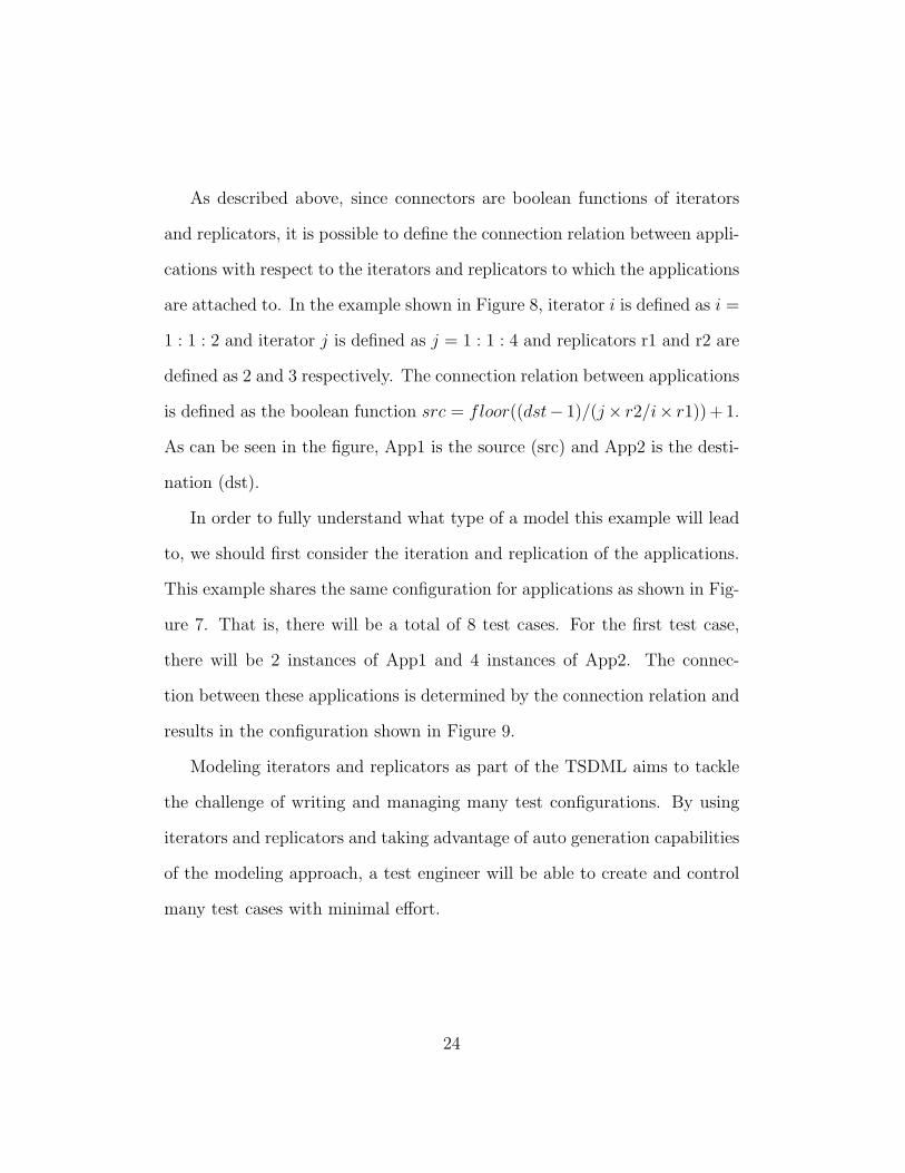
As described above, since connectors are boolean functions of iterators

and replicators, it is possible to define the connection relation between appli-

cations with respect to the iterators and replicators to which the applications

are attached to. In the example shown in Figure 8, iterator i is defined as i =

1 : 1 : 2 and iterator j is defined as j = 1 : 1 : 4 and replicators r1 and r2 are

defined as 2 and 3 respectively. The connection relation between applications

is defined as the boolean function src = floor((dst− 1)/(j× r2/i× r1)) + 1.

As can be seen in the figure, App1 is the source (src) and App2 is the desti-

nation (dst).

In order to fully understand what type of a model this example will lead

to, we should first consider the iteration and replication of the applications.

This example shares the same configuration for applications as shown in Fig-

ure 7. That is, there will be a total of 8 test cases. For the first test case,

there will be 2 instances of App1 and 4 instances of App2. The connec-

tion between these applications is determined by the connection relation and

results in the configuration shown in Figure 9.

Modeling iterators and replicators as part of the TSDML aims to tackle

the challenge of writing and managing many test configurations. By using

iterators and replicators and taking advantage of auto generation capabilities

of the modeling approach, a test engineer will be able to create and control

many test cases with minimal effort.

24

The concept of iterators and replicators easily and conveniently achieve

the parameterization goal of the TSDML and enable creation of series of test

cases from the single test template model.

Modeling Input Generator

Input Generator is an important entity in the TSDML. It is not neces-

sarily part of the overall system however it is crucial to model the input to

the system for testing purposes.

In TSDML, input generator is modeled as a construct containing some

parameters. The input generator is assumed to be used for generating events

for the event based system. The following parameters make up the input

generator:

• Input Generator Parameter: Any parameter that may relate to model-

ing an input generator (e.g. mean, sigma, etc.)

• Random Distribution: Enumeration to model the type of distribution

(e.g. Lognormal, normal, exponential, etc.)

• Parameter Sweeper: Similar to application types, a sweeper can be

connected to parameters to vary the values of parameters for each test

• Iterator Reference: Reference to the iterator used for test series defini-

tion.

25

Most important part of the input generator model is parameter sweeper.

It is the same sweeper that is used for varying values of application pa-

rameters. By connecting the iterator reference to a sweeper, values of input

generator can be varied for each test case to be able to test the system against

varying input data.

Based on the design of the system, the input generator can be connected

to any application which accepts the input data and is the trigger for the

operation of the system. Figure 10 shows the Input Generator portion of the

TSDML metamodel.

Figure 10: Input Generator Meta Model

26

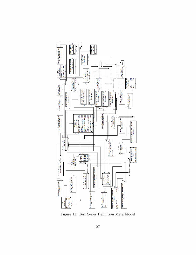
Figure 11: Test Series Definition Meta Model

27

Modeling Test Series Definitions

Test series definition models bring together all the entities of the TSDML

from a test generation perspective and enables generation of series of test

cases utilizing model parametrization described in the previous subsection.

An important advantage of using MIC model based methodology is the

ability to view the system to be modeled from different aspects and enable

separation of design concerns. From this perspective TSDML defines three

different aspects: Test Series Definition Aspect, Deployment Aspect, Perfor-

mance Aspect. All there aspects of modeling a test series definition will be

explained in detail.

The Test Series Definition Aspect includes all the modeling elements

that were described in the previous subsections. Test Series Definition aspect

acts like a design surface for designing series of test cases. It contains the

following modeling elements:

• Application Reference

• Iterator

• Replicator

• Connector

• Input Generator

• Test entity

28

• Connections between these entities

References to application types and connectors that connect the applica-

tions make up the data flow among the applications. In order to create a

test series definition not all application types need to be present. Different

test series definitions with different applications and with same applications

and different parameter values can be modeled since test series definitions

are collected under a folder structure and lead to different set of test cases.

Iterators and replicators are the entities which define the scope of the

series and add parameterization to the test series definition model. As de-

scribed in ”‘Parameterizing the Model”’, a replicator enables using a single

application type and generate multiple application instances during test case

generation. By use of replicators and iterators, it is possible to easily cre-

ate a template of an application to be replicated at each step of test case

generation.

Connector defines the relationship and data flow between the applications.

When a connector entity is used to connect ports of two applications, it

denotes that there is a data flow between those applications. As explained

before, it is also a very powerful entity with its ConnectionRule property

which is a function of the iterator. Making connections this way enables

variations on the application structure that is to be tested.

The InputGenerator entity supplies the test data to the system to drive

the test run. It can be connected to the applications which are expecting

data to be enabled.

29

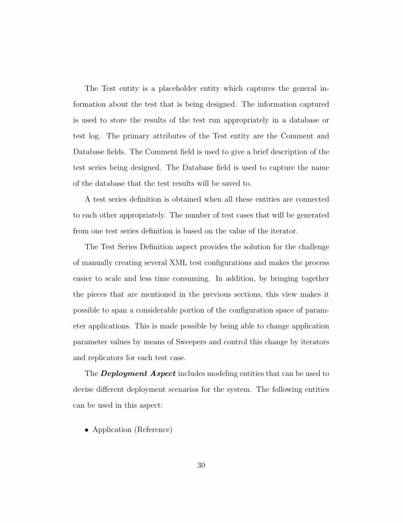
The Test entity is a placeholder entity which captures the general in-

formation about the test that is being designed. The information captured

is used to store the results of the test run appropriately in a database or

test log. The primary attributes of the Test entity are the Comment and

Database fields. The Comment field is used to give a brief description of the

test series being designed. The Database field is used to capture the name

of the database that the test results will be saved to.

A test series definition is obtained when all these entities are connected

to each other appropriately. The number of test cases that will be generated

from one test series definition is based on the value of the iterator.

The Test Series Definition aspect provides the solution for the challenge

of manually creating several XML test configurations and makes the process

easier to scale and less time consuming. In addition, by bringing together

the pieces that are mentioned in the previous sections, this view makes it

possible to span a considerable portion of the configuration space of param-

eter applications. This is made possible by being able to change application

parameter values by means of Sweepers and control this change by iterators

and replicators for each test case.

The Deployment Aspect includes modeling entities that can be used to

devise different deployment scenarios for the system. The following entities

can be used in this aspect:

• Application (Reference)

30

• Resource (Reference)

• Middleware

• Port

Any common entities across aspects are carried over to the respective

aspect. For this reason, the application reference is the same as the on used

in the Test Series Definition aspect. The difference across different aspects

is the perspective those entities are being looked at. While in the Test Series

Definition aspect, the application reference was viewed from the perspec-

tive of creating a test series definition with multiple instances of applications

generated automatically. In this aspect, the applications are viewed from a

deployment perspective. The connections that are to and/or from an appli-

cation reference are related to the deployment aspect of the system.

Resource reference is a reference to any resource that is modeled in the

Resources and Resource Configurations. Deployment aspect is the only place

where a resource can be utilized because it’s inherently related to deployment.

From the testing perspective, having a resource model in this view makes it

possible for a test designer to deploy a system on various resources and devise

several test cases.

Another entity in the Deployment aspect is Middleware. It is a key entity

for deployment because applications cannot run in absence of middleware and

have to be deployed in a middleware instance. Technically, middleware is no

different than an application, it’s defined and modeled with application types.

31

However, it’s special in the sense that can contain other application types.

As applications can be deployed on middleware, middleware is deployed on

resources on specific ports.

Port, as the name suggests, is a logical entity used to define endpoint for

the application on the resource that it is deployed to. It is used to connect

middleware to a resource. Port has the following attributes:

• Port Type: Type of port (e.g. TCP/IP, SOAP, etc.)

• Port Value: Value of port (e.g. 8080, 4000, etc.)

The Performance Aspect includes entities related to capturing per-

formance information about the system. The main entity of this aspect is

the Performance Probe. It’s designed to be analogous to a voltmeter or am-

meter used to measure electric voltage and current in electronic circuits. In

this manner, a performance probe is connected to positive and negative end

points and measures a performance metric between those points.

A performance probe has one attribute:

• Metric: It’s an enumeration of possible performance metrics to be mea-

sured (e.g. throughput, latency, bandwidth).

For example, when a performance probe is connected between the nega-

tive probe end of App1 and positive probe end of App2 and its metric is set

as Throughput, it means that throughput between App2 and App1 will be

measured.

32

All the aspects of the Test Series Definition make up the main parts of the

TSDML. Test series definition uses the modeling constructs defined elsewhere

to model a system from test, deployment and performance points of views.

Modeling Behavior with DEVS

The Test Series Definition Modeling Language makes it possible to model

the system from various perspectives. It is a graphical domain specific lan-

guage that can be used to capture structure and data flow of a system from

a higher level of abstraction. TSDML also enables the design of a system

from the testing perspective.

In model driven engineering, the crucial step after modeling a component

or a system is to be able to interpret the meaning of the abstractions in the

model. The artifact of such interpretation can be a design document, source

code, etc. In the case of the approach described in this chapter and the

TSDML, the desired artifact is several test cases (e.g. in the form of XML

configurations) that can be executed on the real implemented system.

In some cases, the real implementation of the system modeled by TSDML

may not be available. Moreover, it may not always be feasible to execute the

test cases on the real system. An implementation of the system may not

yet be available or it may be costly to run unpredictable tests on the real

implementation or replicate the real system setup for testing purposes. In

such cases, it is important to be able to model the behavior of the system as

well.

33

In the approach described in this chapter, the behavior model of the ap-

plications of the system is created using the Open DEVS modeling formalism.

A background on Open DEVS is given in Chapter III.

DEVS modeling formalism and the underlying simulation framework en-

ables the execution of test cases generated from TSDML on a simulated

system. In order to achieve that, each application type that is modeled using

TSDML should have a corresponding DEVS behavior model. An application

is modeled using DEVS as described in Chapter III. The main aspect of this

process is correctly determining:

• States of the application

• Input and output events of the application

• Input and output connections/ports of the application

Since DEVS is an event based framework, it is possible model the data

flow and interactions among applications. In a middleware based system, it is

particularly important to determine interactions between applications. It is

possible with DEVS to model the application interaction in such a way that

no application can talk to each other without going through middleware.

An example implementation of a DEVS model will be given in Chapter

V.

34

Closing the Loop: Performance Engineering

In Chapter I, it was stated that the scope of the approach described in this

thesis is within the boundaries of designing ”‘test case selection or generation

strategies specifically intended to test for performance criteria rather than

functional correctness criteria”’.

Although the description and the goal is pretty clear and easy to under-

stand, some questions and details are hidden below the surface. Functional

requirements define how the system is supposed to behave whereas non-

functional requirements define the expected operation of the system beyond

the functional behavior, e.g. response time. Non-functional requirements are

harder to gather and define than functional requirements. Similar difficulty

exists in testing non-functional requirements [17]. The difficulty generally

stems from the nature of non-functional requirements being frequently ob-

served and evaluated subjectively. Performance is such a non-functional sys-

tem requirement. Non-functional requirements like performance are usually

evaluated, analyzed or even predicted during design time and rarely moni-

tored and tested during run-time.

The integration of performance analysis with the engineering process is

commonly called as performance engineering. The first approach to inte-

grating performance analysis with development cycle early on has been the

Software Performance Engineering (SPE) methodology. SPE was first in-

troduced by Smith in her seminal work in early 90s [18]. The goal of SPE

35

is to provide guidelines for performance modeling throughout the software

development cycle [19].

In the core of the SPE methodology, there is the domain analysis and

object-oriented development. The models that are created as a result of

the domain analysis are used to predict the performance of software sys-

tems in an early stage. The performance model to be used to implement

SPE methodology depends on the purpose of the analysis. Smith lists three

analysis strategies that guide the model selection [19]:

• Adapt-to-precision strategy: Availability of system information knowl-

edge directs the modeling effort. Using easy to construct models is

suggested.

• Simple-to-realistic strategy: Abstracting away details initially and then

adding more details incrementally as the system evolves is suggested.

• Best-and-worst-case strategy: In the early stages of software develop-

ment, the input data is rarely complete and precise. Thus, investi-

gating performance bounds with best-case and worst-case data sets is

suggested.

The main elements of the SPE methodology are Software Execution Mod-

els and System Execution Models. First, the important aspects of the soft-

ware performance behavior is modeled with execution graphs [18] to form the

Software Execution Models. The execution graphs are then used to generate

36

parameters for the System Execution Model. The system execution model in-

cludes information regarding the hardware resources including queue-servers

and their possible connections throughout the system. Execution scenarios

are formed from these possible connections which form the model workloads.

System execution models are analyzed [20] and the solution results in mean-

value results. The mean-value results are checked against performance goals

and if the performance is not satisfactory, system designers turn back to

models to work on more advanced system execution models [19].

In the previous sections, an approach for modeling a system’s behavior

and structure from performance perspective was described. The approach

described enabled generation of many test cases from TSDML models to

be executed on a discrete-event DEVS simulation engine running behavioral

models of the system. There are two paths that can be taken from the model

level to the system level:

• Test cases may be executed on the real system (Figure 12). Running

test cases on the real system for performance testing potentially gives

the best results. However, this option may not always be available since

it may be costly to run test cases with unpredictable outcomes on a

real system. In such a case, it may be desirable to replicate the real

system in a similar environment which may also be a costly operation.

• Test cases may be executed on a simulation environment using behav-

ioral models for the applications (Figure 13). This path is less costly

37

Figure 12: Test Cases Run on System Implementation

albeit the quality of performance test results are highly dependent on

how closely the system behavioral models capture the design of the

system.

In either case mentioned above, there needs to be a way to make an as-

sessment about the results of the test run. If performance requirements were

clearly captured and each performance metric could be measured at the end

of a test run, it might be possible to make pass/fail decision on the test run.

However, the question is: is it desirable to merely verify performance, or in

general non-functional requirements, in the same manner as functional re-

quirements? One may argue that non-functional requirements testing phase

in the development life cycle is more about observing, understanding how

the system performs in different conditions, environments or with different

system parameters. It is more valuable to be able to analyze test run results,

38

Figure 13: Test Cases Run on Simulation Engine

reason about the system performance, and identify relationship of system

parameters with performance then to make a pass/fail decision. From this

perspective, (performance) testing approaches (performance) engineering. In

this sense, it is crucial to be able to feed the results of a test run back into de-

sign og the system, thus closing the loop. This does not necessarily mean to

automatically feed a test run result back into the system. This feedback may

be in the form of understanding more about the system and devising more

and interesting test cases with variations in system parameters or system

environment.

There is extensive literature on performance prediction from performance

models (e.g. [21], [22], [23]) and those literature was investigated in [12].

However, the approach described here is not about predicting the perfor-

mance of a system from performance models as outlined above. It is im-

portant to make the distinction between creating a performance model for

a system and creating a system model and including a performance aspect.

39

In the approach described here, in a typical model based development sense,

behavioral and structural abstractions of a system are captured in a system

model and this model is extended from performance point of view. Since it is

also possible to generate series of test cases from this system model, it is pos-

sible to run the actual test cases either on the real system or in a simulation

environment to reason about the actual performance of the system.

In order to get information about the performance of the system, a mon-

itoring system is typically needed when this information cannot be obtained

from the system during design time. A monitoring system is used to collect

run-time information about a system [24]. Performance information of a sys-

tem is a typical information that can be obtained during run-time. When the

generated test cases are run on the actual system, obtaining performance re-

sults will rely on the monitoring system in place for the actual system. On the

other hand, when the generated test cases are run on the simulated system,

a performance monitoring component is needed. For the implementation of

the approach, a performance monitor that collects performance information

about the simulation system under test is explained in Chapter V.

A system designer has the knowledge about the internals of the system

and how it should work. If one considers a designer who is designing a

distributed middleware based system, it’s safe to assume that she knows the

structure of the system to be designed, the services the middleware is going

to provide to the applications, how applications will use those services, and

what type of complex interactions will take place between applications and

40

the middleware services. The modeling approach described in this thesis

gives the designer ability to capture her knowledge about the system she is

designing in the form of models. When both the structure and behavior of

the system is captured and either a simulation environment or parts of the

real system is available, the designer can easily explore the behavior of the

system and its effect on the performance of the system.

The approach enables the designer to easily create experiments, Test Se-

ries Definitions, and effortlessly generate test cases to exercise either the

simulated or the real system. Since models also allow the designer to cap-

ture information about configuration parameters of system components, it

is possible to observe how certain values of parameters in a certain system

structure effects the performance of the system. Designer can then analyze

the resulting data from the experiments, compare them to her performance

goals. If the results are not satisfactory, she can turn back to the design

and make changes to engineer the system to the needs of the design. Figure

14 shows the cycle that the system designer will typically go through for

performance engineering the system.

Finally, an important note should be made about validating the simula-

tion models that are used to make design decisions. One of the challenges

mentioned in Section II of this chapter was about having previous versions

of a system. The remark on that challenge was about determining a repre-

sentative workload for the system. However, similar challenge also applies

to having historical benchmark data about a system. If there is historical

41

Figure 14: Engineering Process

42

performance benchmarks for the system, results of performance tests can be

compared against the benchmarks to catch invalid abstractions made in the

simulation models. Results of a test run can be compared against trends

of performance metrics with respect to changes in parameters whose impact

on the system is well known. In addition, designer should always question

the validity of results and should perform sanity checks to consider whether

resulting data makes sense. Another aspect that needs to be considered is

the validity of system behavior models. Performance test results depend on

the DEVS behavior models. Those models are derived from functional re-

quirements of the system. In order to have higher confidence in the validity

of behavioral models, functional testing techniques [25] can be employed.

Summary

In this chapter, a method for performance testing distributed middle-

ware based systems were described. Several challenges including difficulty

of creating many system configurations for a distributed middleware system

were identified. As a possible solution to the challenges identified, a model

based approach was described. Test Series Definition Modeling Language

(TSDML) was presented in detail.

The approach described in this chapter focused on using modeling a sys-

tem from performance perspective. It was pointed out that it was different

43

from research that is focused on creating performance models for perfor-

mance prediction. The modeling approach enabled the use of models during

the system design cycle with an added perspective of performance testing.

In addition to the TSDML, modeling behavior of the system using DEVS

modeling formalism was presented. The connection between the TSDML

and DEVS modeling layers were explained.

Finally, a brief discussion on performance engineering of a system was

given. The discussion focused on clarifying that the goal of the approach

is enable performance engineering of a system based on observations from

experiments conducted on the system using TSDML and DEVS models.

44

CHAPTER III

BACKGROUND ON DEVS MODELING FORMALISM

Discrete Event System Specification (DEVS) is a modeling and analysis

formalism for discrete event systems [8]. Modular and hierarchical modeling

views are two important aspects in DEVS formalism. Modularity is achieved

by input and output events whereas hierarchical aspect is realized by the

coupling operation.

A DEVS system is formed of states, input and output events, a notion

of time, and functions that describe how the system evolves with respect to

input and output events.

There are two types of DEVS models. Atomic DEVS models enable a

system to be modeled modularly by first creating models by simple funda-

mental dynamic behaviors. Coupled DEVS models enables the definition of

the system hierarchically by coupling the atomic models to create a complete

system specification. Mathematical definitions of those models will be given

in the next sections.

Atomic DEVS Models

An atomic DEVS is a 7-tuple structure A =< X, Y, S, s0, τ, δx, δy > [2]

where

• X is a set of input events.

45

Figure 15: Symmetric Structure of Atomic DEVS [2]

• Y is a set of output events.

• S is a set of states.

• s0 ∈ S is the initial state.

• τ ;S → T is the time advance function where T = [0,∞] is the set of

non-negative real numbers plus the transfinite number, infinity. This

function is used to determine the lifespan of a state.

• δx : P × X → S × {0, 1} is the input transition function where P =

{(s, ts, te)|s ∈ S, ts ∈ T, te in[0, ts]} represents the set of states. Times

ts and te are the lifespan of the state and the elapsed time since the last

reset of te, respectively. The booelan result in the definition determines

whether the elapsed time will be reset or not.

Figure 15 shows the structure of an atomic DEVS model. The symmetric

nature of the DEVS model comes from the fact that input event set X and

46

input transition function (δx), and output event set Y , and output transition

function (δy) are on the opposite sides of the structure [2].

There are two types of transitions in an atomic DEVS model: external

and internal transitions. These transitions are the only ways a model can

change its state. Internal transitions are time-based. That is, an internal

transition occurs when the elapsed time reaches to the lifetime of the state

which is defined by τ(s). An internal transition not only causes a state change

but may also generate an output event. External transitions are event-based.

That is, an external transition occurs when an input event arrives. An input

event causes a state change when the conditions given by δx is satisfied.

External transitions are instantaneous and only trigger state change and do

not generate an output event.

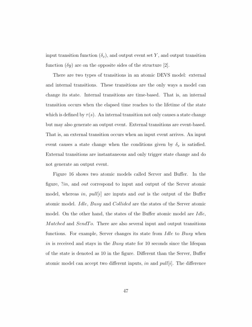
Figure 16 shows two atomic models called Server and Buffer. In the

figure, ?in, and out correspond to input and output of the Server atomic

model, whereas in, pull[i] are inputs and out is the output of the Buffer

atomic model. Idle, Busy and Collided are the states of the Server atomic

model. On the other hand, the states of the Buffer atomic model are Idle,

Matched and SendTo. There are also several input and output transitions

functions. For example, Server changes its state from Idle to Busy when

in is received and stays in the Busy state for 10 seconds since the lifespan

of the state is denoted as 10 in the figure. Different than the Server, Buffer

atomic model can accept two different inputs, in and pull[i]. The difference

47

Figure 16: Atomic DEVS Models [2]

between these inputs will be evident shortly when the Coupled DEVS model

is explained.

Coupled DEVS Models

A coupled DEVS is also a 7-tuple structure [2]

N =< X, Y,D, {Mi} , EIC, ITC,EOC > where

• X is a set of input events

• Y is a set of output events

• D is a set of names of subcomponents

• {Mi} is a set of DEVS models where i ∈ D. Mi can be either atomic

DEVS model or a coupled DEVS model

• EIC ⊆ X × ∪i∈D

Xi is a set of external input couplings where Xi is the

set of input events of Mi.

48

Figure 17: A Coupled DEVS Model [2]

• ITC ⊆ ∪i∈D

Yi × ∪i∈D

Xi is a set of internal couplings where Yi is the set

of output events of Mi.

• EOC ⊆ ∪i∈D

Yi × Y is a set of external couplings.

A coupled DEVS model defines the subsystems that are contained by the

model and how there are connected to each other. Coupled DEVS models re-

alize the modular and hierarchical aspect of the DEVS formalism by enabling

a system designer to build a larger system by designing and connecting sim-

pler subsystems. Although it is not impossible to create a complete system

only with atomic models, it is very tedious and error prone. Coupled DEVS

model eliminates this complexity and lets subsystems be composed together

and connected to each other enabling a better system specification.

49

Figure 17 shows a coupled DEVS model [2]. It’s part of a Client-Server

system. The configuration in Figure 17 is for 3 servers. A buffer is present

to hold requests from clients and coordinate allocation of clients on to the

servers. As mentioned in the previous section, Buffer can accept to inputs

denoted by ?in and ?pull. The in input comes from a client whose model is

not shown here. The pull inputs come from servers and are indexed by the

server in the form of pull[i]. Since this is a coupled system, outputs out1,

out2 and out3 from the Buffer is fed into the input ports of the corresponding

Server. Similarly, output of each Server becomes the pull[i] input for the

Buffer.

Since the resulting DEVS model is modular and hierarchical, events gen-

erated within a subsystems can propagate through other parts of the subsys-

tem horizontally, or through other subsystems vertically within the hierarchy

of the system through well defined interfaces.

Summary

DEVS formalism provides the means to describe discrete event systems

and provides constructs like time, events, states and transitions as well as

composition of models. In this research, DEVS was chosen to be used to

model a distributed data acquisition system from simple atomic models of

system components along with domain specific models. Event-based nature

50

of the data acquisition system made DEVS the proper tool to model its mid-

dleware and applications using the DEVS modeling formalism. The Open

DEVS simulation framework [2] provides suitable ground work to model ap-

plications as DEVS models and simulate the complete system.

51

CHAPTER IV

BACKGROUND ON CMS DAQ SYSTEM

The Compact Muon Solenoid (CMS) experiment is a particle physics

detector built on the proton-proton Large Hadron Collider (LHC) being built

at CERN in Switzerland. One of the goals of CMS is to discover the Higgs

boson. CMS is designed as a general-purpose detector and is going to be

capable of studying results of proton collusions to take place inside the LHC.

An experiment at a hadron collider requires a sophisticated trigger and

data acquisition (DAQ) system because of very high collision and overall data

rates. The frequency of protons crossing each other at the LHC is 40 MHz

[26].

The main goal of the CMS Trigger and Data Acquisition System (TriDAS)

is to inspect the detector information arriving at 40 MHz frequency and to

select events and to store them for offline processing. The events are selected

at the maximum rate of O(102). There are two steps in the functionality of

the system. The first step, which is called the Level-1 Trigger [26], is designed

to reduce the rate of events selected for offline processing to less than 100

kHz. The second step, which is called High-Level Trigger (HLT), is designed

to further reduce the 100 kHz. of the Level-1 Trigger to the final output rate

of 100 Hz.

Functionality of the CMS DAQ and HLT is given in the CMS DAQ Tech-

nical Design Report as follows [26]:

52

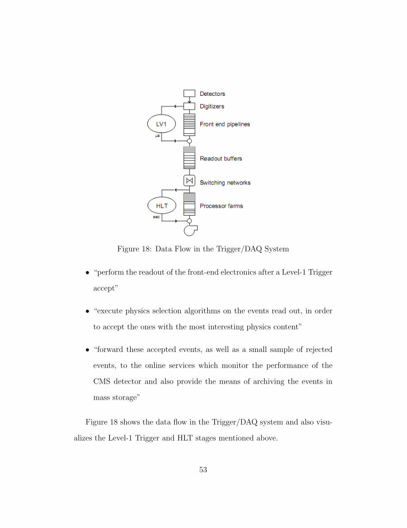
Figure 18: Data Flow in the Trigger/DAQ System

• “perform the readout of the front-end electronics after a Level-1 Trigger

accept”

• “execute physics selection algorithms on the events read out, in order

to accept the ones with the most interesting physics content”

• “forward these accepted events, as well as a small sample of rejected

events, to the online services which monitor the performance of the

CMS detector and also provide the means of archiving the events in

mass storage”

Figure 18 shows the data flow in the Trigger/DAQ system and also visu-

alizes the Level-1 Trigger and HLT stages mentioned above.

53

DAQ Architecture

Figure 19 shows the architecture of the CMS DAQ system. The system

consists of the following elements:

• Detector Front-ends are the components that are connected to the

front-end electronics to store the data from them as the Level-1 Trigger

accept signal is received.

• Readout Systems are the components that are connected to the

Front-End System (FES) to read the data from the detector. Read-

out systems store the data until they are sent to the processor to which

will analyze the event.There are about 500 components which are called

“Readout Columns”. Each Readout Column consists of a number of

Front-End Drivers (FEDs) and one Readout Unit (RU). RU is respon-

sible for keeping the event data in its buffer and interfacing to the

switch.

• Builder Network is a collection of networks providing the inter-

connections between the Readout and Filter Systems. It can handle

800Gb/s sustained throughput to the Filter Systems.

• Filter Systems are the processors that the RUs provide the events

with. Filter systems are the entities that decide whether a supplied

event is interesting and will be kept for offline processing or not. The

interestingness of an event is determined by executing the High-Level

54

Figure 19: CMS DAQ System Architecture

Trigger algorithms. There are about 500 entities which are called “Fil-

ter Columns”. Each of those include one Builder Unit (BU). A BU is

responsible for receiving incoming data fragments that correspond to a

single event and building them into full event buffers.

• Event Manager controls the flow of events in the system. Event Man-

ager (EVM) serves as a centralized intelligence of event management.

• Computing Services are composed of all the processors and networks

that receive filtered events and some of the rejected events from the

Filter Farms.

• Controls are responsible for the user interface and the configuration

and monitoring of the DAQ.

Given the component breakdown of the system it is possible to identify

four stages of system functionally. The first stage is a detector readout stage

55

where events are collected and stored in buffers. The second stage is the event

building stage, where all data corresponding to a single event are collected

from the buffers. The third stage is the selection stage where High-Level

Trigger in the processor processes the event. The final stage is the analysis

and storage stage where the events that are selected in the previous stage

are sent to the Computing Services for additional processing for storage or

further analysis.

XDAQ uses a format called I20 data binary data format. I2O (Intelligent

Input Output) is an I/O architecture specification developed by a consor-

tium of computer companies called the I2O special Interest Group (SIG) for

managing devices. The details of the I2O message format is not in the scope

of this research. However, more information about the details of the I2O

specification may be obtained from [27].

Event Builder

The main task of the DAQ system is to read each event’s corresponding

data out of the FEDs and merge it into the single structure called “physics

event” and to transmit the physics event to a filter farm consisting of pro-

cessor that execute physics algorithms that decide whether the event should

be kept for further processing or discarded [26]. The Event Builder (EVB)

is the central component of the DAQ system and includes the components

that are responsible for this task.

56

Figure 20: Front and Side Views of the DAQ

Figure 20 shows a more detailed version of the DAQ architecture depicted

in Figure 19.

In the first of the stages that were idenfied above, there exist 8 FEDs

that the RUs read data from and perform merging of event data fragments

into larger data blocks called “super-fragments” or “s-fragments”. This ar-

rangement makes up a 64 “FED Builders” each of which consists of 8 FEDs,

a 8x8 switch, and 8 RUs. Readout data is distributed among 64 RUs to

maximize readout bandwidth. Thus, parts of data from a single event are

buffered in 64 RUs. In the second state, 64 BUs which read out the data

from a single event contained in 64 RUs and build these 64 s-fragments to

form a single event. RUs and BUs are connected to each other through a

64x64 switch. The group of 64 RUs, the 64x64 switch and 64 BUs are called

the “RU Builder”. The full XDAQ system is composed of 64 FED Builders

57

Figure 21: Three-Dimensional View of the System

and 8 RU Builders. Figure 21 shows the three-dimensional representation of

the system [26].

RU Builder

This research is mainly interested in the components of the RU Builder

as the experimental platform. Figure 27 shows the event builder and how

the RU Builder is connected to the rest of the system [28].

RU Builder consists of several applications. There is a single Event Man-

ager (EVM), one or more readout units (RUs), and one or more builder

units (BUs). The trigger adapters (TAs), readout unit inputs (RUIs) and

58

filter units (FUs) are external to the RU Builder and are not in the scope of

the experimental platform of this research.

Event Manager (EVM)

EVM is the application that controls the flow of event data through the

RU Builder. Figure 22 shows the internal FIFOs of the EVM and its dynamic

behavior.

In the first step, EVM receives trigger data of an event from the RUI.

In step 2, EVM assigns a free event ID to the trigger data. In step 3, EVM

requests the RUs to readout the event’s data. In step 4, BU asks the EVM

to allocate it an event. In this request, BU may also send an event ID to be

cleared. In step 5, EVM saves the event ID received from BU as a free ID.

In step 6, EVM sends the BU a confirmation of the allocation by sending the

requesting BU the assigned event ID and trigger data of the allocated event.

[28]

Readout Unit (RU)

RU is the application that buffers the s-fragments until there is a BU

request. Figure 23 shows the internal FIFOs of the RU and its dynamic

behavior.

In the first step, RU receives a pair of “event ID/trigger event number”

and asks the RU to readout the data of the assigned event ID. In step 2,

59

Figure 22: Dynamic Behavior of EVM

RUI tells the RU that event’s data is ready to for readout and processing. In

step 3, a RU fills in its fragment lookup table with each s-fragment for which

it received pair for from the EVM. In step 4, BUs request from RUs the

s-fragments of the events that they received confirmation for from the EVM.

In step 5, a RU fulfills the request from a BU with s-fragments retrieved from

the s-fragment from its fragment lookup table and asks the BU to cache the

events data [28].

Builder Unit (BU)

BU is the application that is responsible for event building. Figure 24

shows the internal FIFOs of the RU and its dynamic behavior.

60

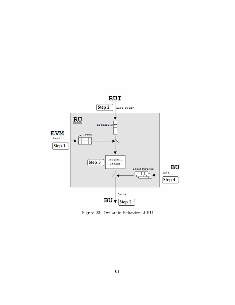
Figure 23: Dynamic Behavior of RU

61

Figure 24: Dynamic Behavior of BU

In the first step, the BU with free capacity asks the EVM to allocate it

an event. In step 2, BU receives the confirmation of event allocation from

the EVM along with the event ID and trigger data of an event which makes

up the first s-fragment of the event. In step 3, the BU asks the RUs for the

rest of the event’s s-fragments. In step 4, the BU receives the the rest of the

event’s s-fragments from RUs, and caches them in its block FIFO. In step

5, the BU builds the event’s s-fragments into one whole event in its resource

table. In step 6, FUs requests an event from BU for processing. In step 7, BU

allocates a whole event to the requesting FUs. In step 8, when a FU finishes

processing an event, it asks BU to discard the event ID corresponding to

processed event [28].

62

Summary

CMS DAQ system is the data acquisition system for the CMS experiment.

In this chapter, basic information about the architecture of the CMS DAQ

system was given. The focus was given on the Event Builder and more

specifically the RU Builder and its applications. RU Builder applications are

used as part of the experimental platform for this research.

63

CHAPTER V

MODEL BASED PERFORMANCE ENGINEERING OF CMSDAQ SYSTEM

In the previous chapters the methodology of the approach was described

along with information on TSDML and DEVS modeling formalism. A back-

ground information about the CMS DAQ system was also given in Chapter

IV. In this chapter, details of the implementation of the approach on the

CMS DAQ system will be explained.

The first section focuses and its subsections focus on describing the system

under test and how it’s broken into layers. The next section describes in

detail how the applications in the system are modeled in DEVS modeling

formalism. The third section talks about the performance aspect captured

in the models. The fourth section explains the implementation of the random

input data generator used to feed data into the simulation system. The next

section lays out the communication interfaces between applications. Section

five describes how the system is modeled in TSDML for test generation.

Sections six and seven focus mainly on performance engineering and analysis

of experiment results.

64

Figure 25: System Architecture

System Under Test

The system that is modeled for performance testing/engineering is a mid-

dleware based distributed system which can be depicted in three layers as

shown in Figure25.

The modeled system is based on the XDAQ framework which is developed

at CERN as a platform for the development of distributed data acquisition

system [26]. A brief background on CMS XDAQ system is given in Chapter

IV

In the upcoming sections, implementation of components of the system

under test will be described. A depiction of the system under test as imple-

mented can be seen in Figure 26.

65

Figure 26: Implementation of System Under Test

Application Layer

There are four applications that exist in the application level. Those are

Event Manager (EVM), Readout Unit (RU), Builder Unit (BU), and Peer

Transport (PT).

Peer Transports are special applications that carry out the data trans-

mission in the distributed programming environment. Data transmission in

XDAQ and Peer Transports are explained in detail in the CMS DAQ Tech-

nical Design Report [26].

EVM, RU and BU applications form the RU Builder which is part of a

larger system called the event builder (EVB). Given the distributed nature

of the EVB, it is responsible with reading event fragments from one set of

66

Figure 27: RU Builder Connected to Event Builder

nodes and assembling them into entire events on another set of nodes. Figure

27 shows the event builder and how the RU Builder is connected to the rest

of the system [28].

This research is interested in the RU Builder and the applications that

make up the RU Builder. Details of all the other components are given in

[26].

67

Event Manager (EVM) is the component which is responsible for deter-

mining the data flow in the RU Builder. Mainly, EVM assigns event id’s to

the events coming into the RU Builder. In addition, EVM manages the life-

time of the event id’s as long as they are in the RU Builder. For this reason,

EVM is the only component that knows about the status of the assigned

event id’s being processed in the RU Builder. EVM is in communication

with all the RUs and BUs in the RU Builder [26].

Readout Unit (RU) is the component which is responsible for reading

super-fragments, keeps them in the memory until there is a request from the

Builder Unit, and transmits the requested super-fragments as a response to

the request [26].

Builder Unit (BU) is the component which is responsible for building

complete events from the super-fragments that are in RUs. As BU builds

complete super-fragments, it keeps them in its buffer until they are requested

by the Filter Unit. Filter Unit is the computational unit of the Filter Farm

which runs the physics algorithms [26].

Middleware Layer

In the XDAQ architecture, the middleware layer is called the Executive

Framework which is basically a XDAQ application called Executive. In a

distributed manner, a copy of the Executive is run on every node that par-

ticipates in data acquisition and event building.

68

Figure 28: Dynamic Behavior and Internal FIFOs of Executive

In the next section, how these application components are modeled in the

context of Open DEVS framework will be explained.

Application Simulation Models

Executive

Executive is the only application that resides in the middleware layer and

is responsible for coordinating the communication of applications. Figure 28

shows the dynamic behavior of the Executive.

Step 1: An application that needs to send an event to another appli-

cation sends the event to the Executive. Upon receipt of the message from

any application on its input port, the Executive saves the message into the

requestBufferFIFO.

69

Step 2: Executive knows about the available PeerTransports to use to

send messages to the desired applications. Executive sends the send event

to the appropriate PT.

Figure 29 shows the DEVS model of Executive with states and input and

output events. Executive has two input and two output ports. The input port

labeled in accepts input from any of the applications whereas in proc accepts

input from the Processor. The output port labeled out sends output to Peer-

Transport application whereas out proc sends output to the Processor. Exec-

utive is initially at WAIT state and stays at the state until there is an input

from an application from the in port. As a request from an application comes

through the in port, Executive switches to SCHEDULE state and immedi-

ately switches to WAITING FOR PROCESSOR after outputting the event

schedule to request T amount of time from the Processor. This event is sent

out from the out proc port to the Processor. When run input event is received

from the Processor while the Executive is at WAITING FOR PROCESSOR

state, the Executive switches to RECEIVE REQUEST state. While at this

state, Executive processes the request from the application until the sched-

uled processor time is elapsed. When the Executive receives the ret event

at the in port from the processor, it immediately switches to the SEND-

ING state. At this state, Executive sends out the processed requests to the

PeerTransport application from out proc. The Executive stays at this state

until all the requests are sent out, that is sendQueue is empty. As soon as

sendQueue is empty, the Executive goes back to the WAIT state.

70

Figure 29: Executive Model

71

Figure 30: Processor DEVS Model

Processor Model

The experimental framework also includes a processor model to imple-

ment simple scheduling. Figure 30 shows the DEVS model of the processor

along with it states, transition conditions and inputs and outputs.

Processor has as many input and output ports as there are applications.

The input and output ports are named as in i, ...in n and out i, ...out n. In-

put and output ports are indexed by application IDs. This way the Processor

knows the application that is making the request. The processor is initially

at IDLE state and stays at that state until it receives an input event at one

of the input ports. When the Processor receives a scheduling request from

an application, it switches to SCHEDULE state. Along with the scheduling

request, application also sends the amount of time it requests. The processor

buffers all the scheduling requests. The Processor immediately leaves the

72

SCHEDULE state and outputs run event and switches to RUN state. The

run event is sent out from the output port whose index corresponds to the

index of the input port on which the request was received. The processor is

set to stay at the RUN state for the amount of time, t RUN, requested by

the application. When this time is elapsed, the Processor outputs ret event

from the same output port the run event was sent out. At this time, the

Processor switches back to the IDLE state.

Event Manager (EVM)

EVM is responsible for controlling the flow of event data in the system.

In the meantime, the EVM assigns event id’s to the events that are gen-

erated. For the purposes of simulation, dummy event data is generated by

the component called InputGenerator. Details of the InputGenerator will be

explained later.

Figure 31 shows the dynamic behavior of the EVM and the input/output

events that it exchanges with the other applications.

Step 1: When the system is enabled the first event that the EVM re-

ceives is the bu allocate clear event from the BU. Since there are no event

requests available at the beginning, this event triggers the operation of the

RU BUilder. Receipt of this event affects the clearedEventId and request

FIFOs of EVM. The incoming event may be for a new event id request, be

a request for release of a used event id, or be a request for both release of

73

Figure 31: Dynamic Behavior and Internal FIFOs of EVM

a used event id and a request for new event id. Upon receipt of the event,

appropriate FIFOs are filled.

At the same time, the initial request for event data is sent to the DataGen-

erator component. Along with the request, a parameter called nbCredits is

sent. This denotes the number of available free event id slots in the builder.

In this first step, the number of available free event id’s is the size of the

freeEventIdFIFO.

Step 2: If there were a request to release an event id in the previous

step, the freeEventIdFIFO is populated with the released event id.

Step 3: EVM asks for new event data with the number of released event

id’s as nbCredits from the DataGenerator.

74

Step 4: DataGenerator sends the generated dummy event data to the

EVM. Upon receipt of the data, dummyDataFIFO is filled with the event

data.

Step 5: If dummyDataFIFO and freeEventIdFIFO is not empty then

pairFIFO is filled with the free event id from the freeEventIdFIFO and the

event number from the dummyDataFIFO.

Step 6: When the conditions for Step 5 are satisfied EVM also sends

ru readout event to RU with the event id/event number pair.

Step 7: If the requestFIFO is filled with a request from BU, and the pair-

FIFO is filled with a Event Id/Event Number, then EVM sends bu confirm

event.

Figure 32 shows the DEVS model of EVM with states and input and

output events.

EVM has two input ports and two output ports. Input port in receives

input events from BU and in proc receives input events from the Processor.

Output port out sends output events to RU and out proc sends output events

to the Processor.

Initially, EVM is in WAIT state until an event is received. When EVM re-

ceives bu allocate clear event from BU and immediately switches to SCHED-

ULE state. It immediately switches to WAITING FOR PROCESSOR and

outputs schedule event at the out proc port. EVM stays at this state un-

til run event is received from the Processor at the in proc input port. At

this time, EVM switches to FILL RQST AND DISCARD FIFO and starts

75

Figure 32: EVM Model

76

processing the input received from BU. EVM stays at this state as long as

ret event is received from the Processor at the in proc port. At this time,

EVM switches to SENDING state and sends out bu confirm event at the out

port to RU. EVM stays in this state until all the events are sent out and

sendQueue is emptied. At this time, EVM switches back to WAIT state.

The events and state transition conditions are clearly indicated on the

figure. EVM implements a queue called sendQueue which is filled in when

there is an output event to be sent out.

Readout Unit (RU)

Readout unit is responsible for gathering the event data fragments and

building super-fragments from them. Multiple fragments make up one com-

plete event. DataGenerator generates dummy events with random fragment

sizes. Figure 33 shows the dynamic behavior of RU.

Step 1: The first step in the RU processing is the receipt of ru readout

event from EVM. EVM sends RU a event id/event number pair for process-

ing. RU populates its pairFIFO with event id/event number pair.

Step 2: RU asks the DataGenerator to send it the fragments of the event

data that corresponds to the event number received from EVM.

Step 3: DataGenerator sends RU the number of blocks that fragment

for the specified event number is composed of. Upon reciept of the data the

blockFIFO of RU is filled with the blocks received from the DataGenerator.

77

Figure 33: Dynamic Behavior and Internal FIFOs of RU

In addition, at the same time, all blocks belonging to a single event are

collected together to form event super-fragments.

Step 4: If the super-fragments are formed and pairFIFO is holding event

id/event number pairs, then the table that is indexed by the event id from

the pairFIFO and that holds all super-fragments is filled with super-fragment

block.

Step 5: BU sends ru send event to request an event super-fragment to

build. Upoxn reciept of the event, requestFIFO corresponding to the index

of the BU that is requesting an event is populated.

78

Figure 34: RU Model

Step 6: If any of the requestFIFOs is filled with a request, RU services the

BU request with event super-fragments that are saved in the super-fragment

table and sends out the bu cache event to BUs that requested an event.

Figure 34 shows the DEVS model of RU with states and input and output

events.

79

RU has two input ports and two output ports. Input port in receives

input events from EVM and BU and in proc receives input events from the

Processor. Output port out sends output events to BU and out proc sends

output events to the Processor.

Initially, RU is in WAIT state. When RU receives an input event from

either EVM or BU at port in, RU switches to SCHEDULE state and immedi-

ately switches to WAITING FOR PROCESSOR as it outputs schedule event

to the at the out port to the Processor. As RU receives the run event from

the Processor at the in proc port, depending on the input received initially at

the in port it either switches to FILL PAIR FIFO or to FILL RQST FIFO.

At these states, RU processes the requests until ret event is received from

the Processor at the in proc port at which time RU switches to SENDING

state. RU stays at this state and sends bu cache event to BU. When RU

finishes all the events in its sendQueue and switches back to WAIT state.

Builder Unit (BU)

Builder Unit (BU) is responsible for building events An event is composed

of one super-fragment from coming from the DataGenerator and N RU super-

fragments where N is the number of RUs. Figure 35 shows the dynamic

behavior of BU.

Step 1: As BU is enabled, the first action it takes is to send initial event

requests to EVM. At this point the builder is completely available to build

events. BU sends the event bu allocate clear event to EVM.

80

Figure 35: Dynamic Behavior and Internal FIFOs of BU

Step 2: BU receives the bu/confirm event from EVM. Upon receipt

of the event, BU fills in the eventIdFIFO with the id’s of events that are

assigned to the system by EVM.

Step 3: If the eventIdFIFO is not empty, BU starts the construction of

the event with the first event id in the eventIdFIFO and is ready to receive

fragments of that event from RUs. At this point, BU sends out the ru send

event to all RUs that are participating in the event building and asks for the

fragments of the event that is under construction. Moreover, at this step, if

a construction of an event is complete, then the fullResourceFIFO is filled

by BU. This also increases the number of events built in the builder, and

completes the lifecycle of an event id/event number pair.

81

Step 4: BU recieves the bu cache event from participating RUs. Upon

receipt of this event, BU fills in the blockFIFO with blocks of event under

construction.

Step 5: If there is an event data block in the blockFIFO then BU ap-

pends event block data to the previous blocks of the same event data. When

the event building is complete the number of events built in builder is in-

cremented and the completed event block is put into the fullResourceFIFO.

In addition, the completed event id ends its lifecycle and is pushed into the

discardFIFO.

Step 6: In the simulation system, there is no Filter Unit to process the

physical importance of those events. Instead the all the events are dropped

after being completed and the number of events built in BU is incremented.

Step 7: If the discardFIFO is not empty then the used event id is recycled

and bu allocate clear is sent to EVM if the total number of events to be built

has not been reached.

Figure 36 shows the DEVS model of BU with states and input and output

events.

BU has two input ports and two output ports. Input port in receives input

events from EVM and RU and in proc receives input events from the Pro-

cessor. Output port out sends output events to RU and EVM and out proc

sends output events to the Processor.

Initially, BU is at WAIT state. When BU receives input events from

either EVM or RU, it switches to SCHEDULE state and immediately sends

82

Figure 36: BU Model

83

Figure 37: Dynamic Behavior and Internal FIFOs of PT

out the schedule output event to the Processor at the out proc and switches

to WAITING FOR PROCESSOR state. When the run input event is re-

ceived from the Processor at the in proc, BU switches to either ENABLE,

FILL BLOCK FIFO FILL EVENT ID FIFO depending on the input event

to be processed. BU switches to SENDING as it receives the ret input event

is received from the Processor at the in proc port. At this state, BU sends

out output events to BU and EVM amd switches back to WAIT state as

soon as its sendQueue is empty.

Peer Transport (PT)

PeerTransport is the component that is responsible for transmitting mes-

sages between applications. Figure 37 shows the dynamic behavior of the

PeerTransport.

Step 1: PT receives send event from the Executive. Upon receipt of the

event, PT fills in the msgBufferFIFO. At this point, PT knows about the

84

communication parties and the message that is being transmitted between

them.

Step 2: If the message buffer is not empty, PT puts the messages in

the buffer into the sendQueueFIFO and sends out the message received from

the Executive to all the applications. PT does not know the contents of

the message or the event that is being transmitted. PT only transmits the

message to all the applications and only the application with the id that

matches the destination id of the message processes the event.

Figure 38 shows the DEVS model of PT with states and input and output

events.

PeerTransport has two input ports and as many output ports as there

are applications. Input port in receives input events from the Executive and

in proc receives input events from the Processor. Output ports out i are

indexed by IDs of applications and send output events to applications and

out proc sends output events to the Processor.

Initially, the PeerTransport is at WAIT state. When send event is re-

ceived from the Executive at the in port, it switches to SCHEDULE state

and immediately sends schedule event to the Processor at out proc port and

switches to WAITING FOR PROCESSOR state. When the PeerTransport

receives run event from the Processor at the in proc port, it switches to

TRANSMIT state. At this state, PT processes the request from the Execu-

tive. When ret input event is received at this state, PeerTransport switches

to SENDING state and transmits messages to the requesting application at

85

Figure 38: PeerTransport Model

86

the output port whose index matches the ID of that application. After all

messages are sent out and its sendQueue is empty, PeerTransport switches

back to WAIT state.

Performance Aspect in Models

DEVS models of applications are given in the previous sections. It’s also

important to note that some parameters related to the performance of the

system are also captured in the application models. These parameters are

mainly parameters of RU Builder applications.

The XDAQ system is distributed as a software package by CERN which

does not allow tuning of performance or modification of any performance

related parameters. The tuning is done by the developers for only the case

for which the system is going to be deployed for the experiment. However,

for the purposes of this research, it was crucial to know the parameters which

are highly probable to have an impact on the system performance.

Upon conversations with XDAQ developers, it was made clear that so

called packing parameters, and total number of blocks that make up a s-

fragment are among the most important parameters that affect the perfor-

mance of the system. In the original XDAQ system all packing parameters

are set as 8. Fragment sizes change during operation as different events have

differing amounts of data.

87

Packing parameters are captured in EVM and BU models. EVM has

the parameter RU READOUT PACKING which determines how many re-

quests need to be packed before sending a readout request to RUs. BU

has the parameter EVM ALLOCATE CLEAR PACKING which determines

how many requests need to be packed before requesting or releasing an event

id and RU SEND PACKING which determines how many requests need to

be packed before sending s-fragment requests from RUs.

In addition to the packing parameters, BU model captures blockFIFOCa-

pacity, requestFIFOCapacity, and maxEvtsUnderConstruction which deter-

mines the maximum number of events that can be constructed in BU.

Varying event data block sizes are not captured in the application models

but rather in the data generator which is explained in the next section.

Input Data Generator

The experiment platform and the simulation engine is driven by a dummy

input data generator. As stated in the previous section, differing event data

fragment sizes are generated by the dummy data generator and fed into the

system.

The input data generator is modeled both in TSDML and simulation. The

important aspects of the input data generator that are captured in TSDML

are:

88

• RandomDistribution: Enables selection of the type of distribution that

is wanted to be used

• BlockSize: According to [26], block size of an event is 4 kB and has

to be captured in the so that it can be varied if needed. Number of

blocks in s-fragment is a statical distribution since different events have

different amounts of data [26].

• NumberOfDataSources: In the CMS system, there are actually 8 total

number of data sources. In order to simulate this behavior, this is also

captured in TSDML.

• EventSizeMean: Average size of an event is 1 MB [26]. This is captured

in the TSDML so that event mean can be varied and the system can

be tested with varying mean event sizes.

• EventSizeSigma: Standard deviation for the event size.

Capturing the input data generator abstractions in TSDML also enables

varying the input data parameters using a sweeper. This is illustrated in

Figure 39.

The core part of the input data generator is implemented as part of the

simulation. However, it is not implemented as a DEVS model and rather im-

plemented as a stand alone component. The type of random distribution is

selected from the TSDML model and can be normal, log normal, exponential

89

Figure 39: Sweeping EventSizeMean and EventSizeSigma

or uniform. Boost Random library is used to generate a random distribu-

tion [29]. For the random distribution generation Mersenne Twister random

number generator is used. The following code snipped demonstrates how a

log normal distribution was generated:

//Create a Mersenne twister random number generator

static mt19937 rng( static_cast<unsigned> (time(0)) );

//Select distribution

lognormal_distribution<double> lognorm_dist(

_eventSizeMean, _eventSizeSigma);

In addition to generating random distribution, input data generator com-

ponent is also responsible for generating event numbers and super fragments

to be consumed by the system. Figure 40 shows how the input data generator

component fits with the rest of the DEVS models.

90

Figure 40: Input Data Generator Component View

Input data generation is triggered by EVM. Number of random event sizes

based on the selected distribution is generated. The total number of event

sizes generated depends on the total number of events that can be built by

XDAQ. EVM also triggers the super-fragment building from the generated

event sizes. A super-fragment is a collection of fragments. In XDAQ system,

an event is composed of several blocks (4KB each) because of the distributed

nature of the system. The goal of super-fragment building is to collect all

blocks of an event into one chunk called a super-fragment. The input data

generator represents a super-fragment as a structure with the following fields:

• Event Number

• Super-fragment Size = Event Size / Number of Super-fragments

• Number of Blocks in Super-Fragment = Super-Fragment Size / Block

Size

91

• Super-fragment Number

• Event data blocks

In the above structure, the fields Super-fragment size and Number of

Blocks In Super-fragment depend on the random event size data generated

by the input generator. Event Size is the size that is generated with selected

random distribution. Number of Super-fragments equals to the total number

of RUs in the system. As can be observed, super-fragment is distributed

equally among all RUs.

In summary, the input data generator generates input event data that

is distributed according to a selected random distribution type and provides

a representation of event data in the form of a super-fragment. A super-

fragment for a specific event number/event id pair is what is consumed by

the simulation engine during a test run.

Performance Monitor

Figure 58 shows a component called Performance Monitor. Similar to the

Input Generator, this component is not part of the models and it’s indepen-

dently responsible for collecting performance data from the system. As seen

in Figure 58, it has the responsibility of saving performance results into the

database as well.

Although the Performance Monitor is not part of the models, it operates

hand in hand with performance probes. Performance monitor is only invoked

92

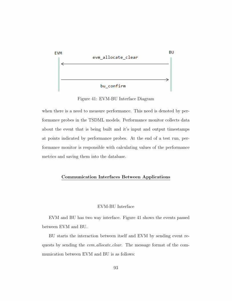
Figure 41: EVM-BU Interface Diagram

when there is a need to measure performance. This need is denoted by per-

formance probes in the TSDML models. Performance monitor collects data

about the event that is being built and it’s input and output timestamps

at points indicated by performance probes. At the end of a test run, per-

formance monitor is responsible with calculating values of the performance

metrics and saving them into the database.

Communication Interfaces Between Applications

EVM-BU Interface

EVM and BU has two way interface. Figure 41 shows the events passed

between EVM and BU.

BU starts the interaction between itself and EVM by sending event re-

quests by sending the evm allocate clear. The message format of the com-

munication between EVM and BU is as follows:

93

address#sourceId#destinationId#event#data

BU sends the following data along with the event:

• buAddress: The IP address of the computer that the BU is running

on

• buId: Unique identifier of the source application, BU

• destinationId: Unique identifier of the destination application

• eventName: Name of the event which is evm allocate clear in this

case

• data: Actual request message which consists of the request.

In order to form the request data, BU sets the following parameters:

• BU Id: The unique identifier of the BU that is making the request.

• Number of Requests Packed: BU does not send one request at a time

but packs multiple requests into one request. The total number of

requests are sent as part of the request data.

• Request type: 0 means event id request, 1 means releasing an event id

and requesting another, and 2 means releasing an event id.

• Event Id: Event id to be released. If requesting an id, this is not need

to be set.

94

• Event Number: Event number that is associated with the released event

id. If requesting an id, this is not need to be set.

• Resource Id: The resource id of the BU that is making the request.

EVM receives the request from the BU and acts on it. As a result,

EVM sends out the bu confirm event to the requesting BU. EVM sends the

following data along with the event:

• evmAddress: The IP address of the computer that the EVM is run-

ning on

• evmId: Unique identifier of the source application, EVM

• buId: Unique identifier of the destination application, BU

• event: Name of the event which is bu confirm in this case

• data: The confirmation message to BU

In order to for the confirmation data, EVM sets the following parameters:

• Event Number (eventNumber): Event number assigned to BU

• Number of Blocks In super-fragment (nbBlocksInSuperFrag-

ment): Number of blocks that make up the sfragment

• Block Number (blockNb): The position of the current block in the

sfragment. It is set as 0 at this time.

95

Figure 42: EVM-RU Interface Diagram

• Event Id (eventId): Event id that is assigned to the BU.

• Super-fragment Number (superFragmentNb): The number of

the super-fragment in the block. Set as 0 for the first set of data.

EVM-RU Interface

EVM and RU has a one way interface. Figure 42 shows the interaction

between EVM and RU.

EVM sends RUs the readout event. The message format of the commu-

nication between EVM and RU is as follows:

address#sourceId#destinationId#event#data

EVM sends the following data along with the event:

• Number of Elements Packed: Total number of read out requests

that is packed. EVM doesn’t send events one by one. Multiple read

out requests are sent.

96

Figure 43: BU-RU Interface Diagram

• Event Id: Event id to be read out from the data generator.

• Event Number: Event number of the data that is read out from the

data generator.

BU-RU Interface

BU and RU has a two way interface. Figure 43 shows the interaction

between BU and RU.

The message format of the communication is as follows:

address#sourceId#destinationId#event#data

BU sends RU the ru send event. BU sends the following data along with

the event:

• Event Id: Event id of the event that BU is requesting

• Event Number: Event number of the event that BU is requesting

97

• BU Resource Id: Resource id of the BU that is going to build the

event

• BU Id: Unique identifier of BU that is requesting the event data

RU sends BU the ”bu cache” event. RU sends the following data along

with the event:

• Block Number: The current block number of the event data in the

data chain

• BU Resource Id: Resource id of the BU that is going to build the

event

• Event Id: Event id of the event that BU is requesting

• Event Number: Event number of the evet that BU is requesting

• Number of Blocks in Super-fragment: Total number of blocks

that make up the s-fragment

• Super-fragment Number: The current s-fragment number in the

s-fragment chain

Application-Executive-PT Interface

The Executive has one way interface with all the applications. Figure 44

shows the interaction between applications, executive, and peer transport.

98

Figure 44: Executive-Peer Transport Interface Diagram

Since applications need to go through the Executive to pass data to other

applications, the above mentioned communication should go through the

Executive.

Executive sends PT the send event. The message format is the same

as given above since Executive does not need any extra information and

transmit the data without making any modifications to it. Executive sends

the data received from the application along with the event.

PT has one way interface with the the applications. PT sends the desti-

nation application the original event that is being transmitted between the

applications. PT does not also make any modifications to the data being

transmitted.

Application-Processor Interface

Processor has two-way interface with all the applications. All applications

go through the Processor for scheduling processing time. Figure 45 shows

the interaction between applications and the Processor.

99

Figure 45: Processor-Application Interface

Applications send the Processor the schedule event when they request

scheduling. Applications send the requested amount of time along with the

event.

Processor sends the requesting application the run event to notify it to

start running. Processor does not pass any data along with the event.

Processor sends the scheduled application the ret event to notify that the

time is up and the application should return. Processor does not pass any

data along with the event.

Test Generation from TSDML Models

In Chapter II, a description of Test Series Definition Modeling Language

(TSDML) and how different components of the system under test can be

modeled. This section will give an example implementation of TSDML for

test generation and provide more details on the process which was shown in

Figure 13 in Chapter II.

Test generation from TSDML models is a crucial part of the approach.

One important challenge for performance testing was mentioned in Chapter

100

II as the need to create many configurations to configure functional operation

of system components. This challenge is addressed in test generation from

models. Before diving into the implementation details, it’s important to

point to some important principles at work in this approach.

The problem of automatically generating many test cases from TSDML

models that this approach is tackling is multiple folds. If there were no graph-

ical tools available for a system designer to design test cases, the solution for

the designer would be crafting various test cases, usually in XML, by hand.

This operation would probably involve many copy and paste operations and

the amount and quality of the test cases would largely depend on the amount

of time that the designer could afford for testing. Moreover, the quality of

test cases could suffer because most of designer’s effort would go into actually

producing the test cases than actually thinking about the efficiency of them.

There could definitely be very good manually created test cases but the error

proneness of the process could hinder the effort.

Introduction of a graphical modeling tool to replace manually writing

XML test cases, as done in the approach described here, is a big improvement

over the manual effort. The process is less error prone and potentially faster

compared to typing and the representation is more readable than an XML file.

However, merely using a graphical modeling tool does not solve the problem

completely. It solves the problem of generating many XML test cases from

the high level representation. On the other hand, it carries some of the

problems associated with the manual effort to the graphical medium. For

101

example, copying and pasting of lines of text in an XML file is replaced with

copying and pasting of boxes on a graphical surface. The system designer

should still take care of creating as many boxes as she needs and configuring

each box which represents an application with its parameters. Moreover,

there is now an even more tedious task of connecting many boxes to each

other correctly. A typical test scenario for a distributed middleware based

system is testing how the system reacts to changes in size. The system

designer would most probably like to create many applications on the design

surface, connect them up and test to observe how the system would scale.

Dragging and dropping boxes on a graphical surface does not make the life

of the system designer easier than a manual effort.

The problem now becomes not only how to generate many test cases at

once but also how to generate many variations of a test case from a single

model of a test. If the goal is to design a test model to test for scaling the

system, there has to be a way to achieve this from a single model instead

of creating one test model for every size of the system that is desired to be

tested. approach described in this thesis attempts to solve this problem by

parameterizing the test models and view them as ”series of tests” thus the

so called ”Test Series Definitions”.

The main premise of the solution is the use of the modeling constructs

called Iterators, Replicators, Connectors and Sweepers. These constructs

enable parameterization of a test model and effectively turn it into a test

series definition. Details of these modeling constructs were given in Chapter

102

II. Each and combination of these constructs attempt to solve the parts and

whole of the problem mentioned above. Sweepers are used to vary parameter

values. Connectors are used to define rules to determine which instances of

applications will be connected to each other, Replicators are used to replicate

the model elements, usually applications, as many as desired. Iterators are

used to drive the generation of many test cases from a single test series

definition.

In the following sections, usage of these constructs along with other mod-

eling elements will be demonstrated as the approach is implement on the

CMS DAQ System.

Constructing a Test Series Definition

In order to demonstrate an example TSDML model, construction of a test

series definition for generating several test cases to experiment with different

event sizes will be described from the ground up.

Application Types

In order to construct a test series definition, applications that will be used

in the definition should be created in the Type Library. Applications that

are required for the test system are EVM, BU, RU and PT. The entities that

are required to model an application type is already described in Section II

of Chapter II.

103

Figure 46: Application Type Model for EVM

Parameters of application types that are used in application type mod-

els come from [28]. Some changes to the organizations of these parameters

where appropriate to help with test generation. All application types have

bi-directional communication ports to all other applications. In addition, ap-

plication types include positive and negative probes as well. Figure 46 shows

the modeling of EVM application as an application type.

It’s important to note that application types are modeled without any

parameter values. This way, when an application type is used (instantiated)

104

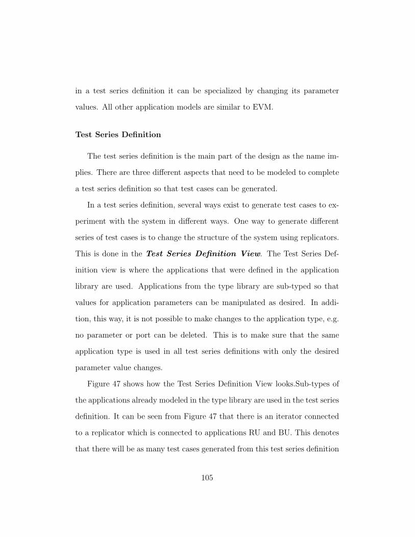
in a test series definition it can be specialized by changing its parameter

values. All other application models are similar to EVM.

Test Series Definition

The test series definition is the main part of the design as the name im-

plies. There are three different aspects that need to be modeled to complete

a test series definition so that test cases can be generated.

In a test series definition, several ways exist to generate test cases to ex-

periment with the system in different ways. One way to generate different

series of test cases is to change the structure of the system using replicators.

This is done in the Test Series Definition View. The Test Series Def-

inition view is where the applications that were defined in the application

library are used. Applications from the type library are sub-typed so that

values for application parameters can be manipulated as desired. In addi-

tion, this way, it is not possible to make changes to the application type, e.g.

no parameter or port can be deleted. This is to make sure that the same

application type is used in all test series definitions with only the desired

parameter value changes.

Figure 47 shows how the Test Series Definition View looks.Sub-types of

the applications already modeled in the type library are used in the test series

definition. It can be seen from Figure 47 that there is an iterator connected

to a replicator which is connected to applications RU and BU. This denotes

that there will be as many test cases generated from this test series definition

105

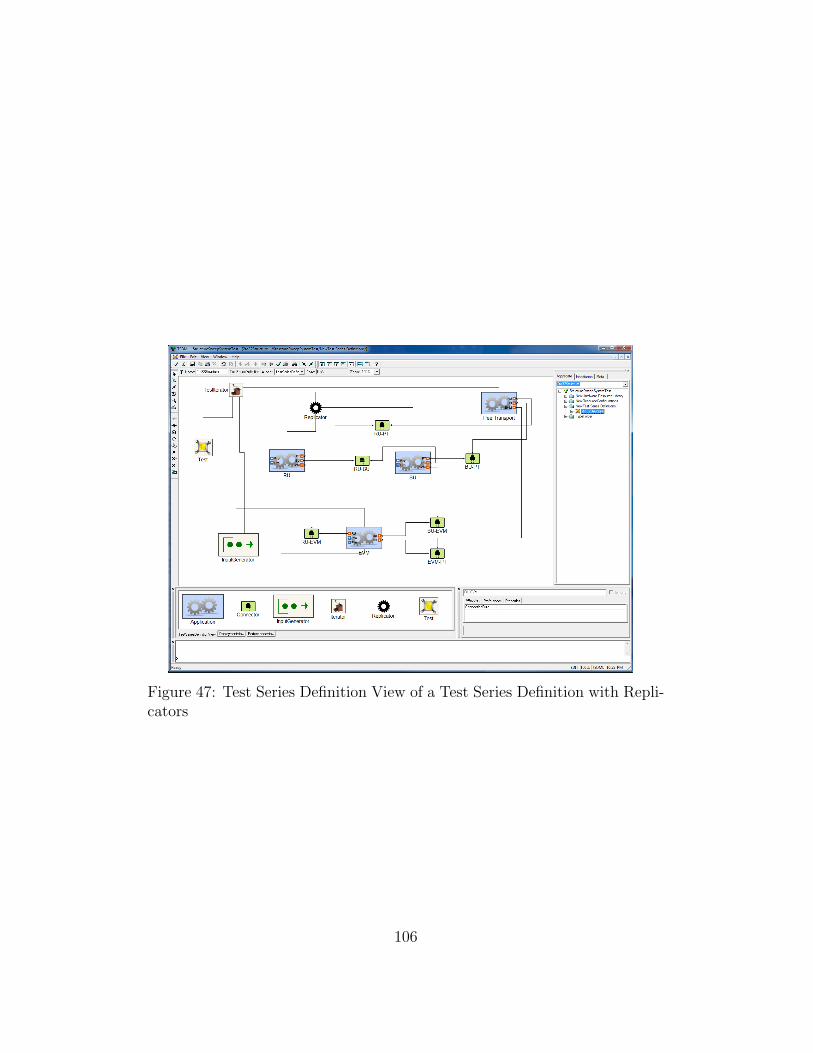
Figure 47: Test Series Definition View of a Test Series Definition with Repli-cators

106

Figure 48: Iterator and Replicator Values

as the value of the Iterator. Moreover, in each of these test cases, applications

RU and BU will be replicated by the value of the replicator. In this specific

example, in each test case the instances of RU and BU will be doubled.

Figure 48 shows the values of the Iterator and the Replicator. It’s important

to note that only the applications RU and BU will be replicated in generated

test cases since the Replicator is only attached to these applications.

In the replication process, in addition to application instances, connec-

tions between applications need to be replicated as well. For this purpose,

several Connectors are used to connect the applications on their bi-directional

ports. In this test series definition, all applications are connected to each

other. As can be seen in Figure 49, the Connector between applications RU

107

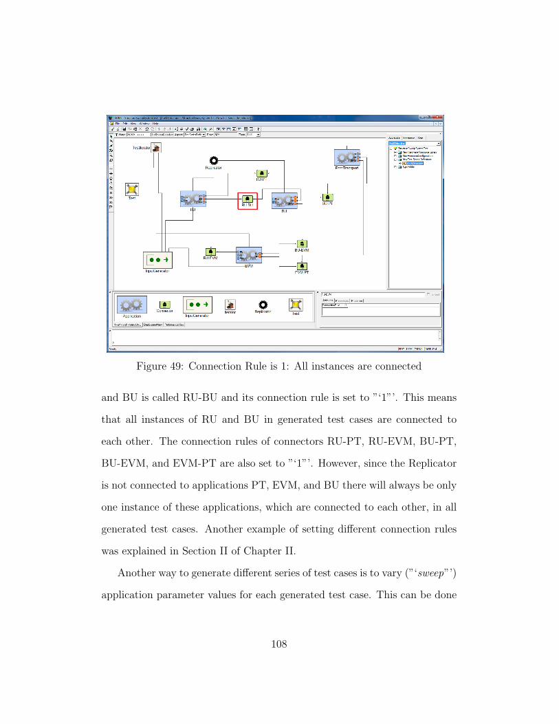
Figure 49: Connection Rule is 1: All instances are connected

and BU is called RU-BU and its connection rule is set to ”‘1”’. This means

that all instances of RU and BU in generated test cases are connected to

each other. The connection rules of connectors RU-PT, RU-EVM, BU-PT,

BU-EVM, and EVM-PT are also set to ”‘1”’. However, since the Replicator

is not connected to applications PT, EVM, and BU there will always be only

one instance of these applications, which are connected to each other, in all

generated test cases. Another example of setting different connection rules

was explained in Section II of Chapter II.

Another way to generate different series of test cases is to vary (”‘sweep”’)

application parameter values for each generated test case. This can be done

108

Figure 50: Sweeping Application Parameter Value

109

using a Sweeper. Sweeper is present in the Test Definition View of an appli-

cation model in the Test Series Definition. Figure 50 shows usage of Sweeper

to generate test cases with varying value for the RU SEND PACKING. The

Sweeper has a function to double the value of RU SEND PACKING. Sweeper

is also connected to a reference to the Iterator of the Test Series Definition

which ensures that the value of the parameter will be doubled for each gen-

erated test case.

Similar to varying application parameter values, Sweeper can also be used

to vary parameters of the Input Generator of the Test Series Definition. This

is especially useful to experiment with varying event sizes. Figure 51 demon-

strates how this is done. As can be seen in the figure, for each generated test

case, mean of event size will be increased by 4 megabits.

Also in the same figure, the RandomDistribution entity can be seen. Input

Generator will create random event sizes with the selected random distribu-

tion type.

So far a test series definition is defined from the Test Series Definition

View which enabled creating variations on the system structure and behavior

to generate series of test cases. Another aspect of creating a test series

definition is deployment. The Deployment View enables deploying the

system. In order to start a deploying the applications, a Node in Resource

Library needs to be modeled. Figure 52 shows a simple model of a node in

the resource library.

110

Figure 51: Sweeping Event Size in Input Generator

111

Figure 52: Model of a Node in Resource Library

112

Figure 53 shows a possible deployment for the test series definition under

construction. The deployment view has a reference to the node that is created

in the resource library. All the applications that were modeled in the Test

Series Definition view are also visible in Deployment View and they are all

connected to the Executive. The Executive represents the middleware layer

which applications need to be deployed on in order to operate. The Executive

also needs to be deployed on a node through a port on which it will run. As

can be seen in Figure 53, the Executive is connected to the Port which is

connected to the NIC of Node1. It’s important to point out that Port is

a logical entity and models the endpoint which will be available to run the

Executive on Node1.

Test Series Definition View and Deployment View covered the behav-

ioral/configuration and deployment aspects of the test series definition. Per-

formance View is where the performance related aspects are added. The

main entity in the Performance View is the Performance Probe. Figure

54 shows how performance probes are connected to indicate measurement

points.

In this specific example, one performance probe is connected to a negative

probe end of application RU and the positive probe end on the application

BU. This denotes that a performance measurement for a selected metric will

be made between the output of RU and the input of BU. Another perfor-

mance probe is connected between the negative probe end of application BU

and positive probe end of application EVM. This denotes that a performance

113

Figure 53: Deployment View of Test Series Definition

114

Figure 54: Performance View of Test Series Definition

115

Figure 55: Metric Choices for Performance Probe

measurement for a selected metric will be made between the output of the

application BU and the output of EVM. Figure 55 shows a more through use

of performance probes.

Test Case Generation

Application simulation models and TSDML models are created. These

models represent the behavioral, structural, and performance aspects of the

system under test under the described abstractions. As described throughout

116

Figure 56: Test Generation Process

this thesis, TSDML models will be used for generating series of test cases to

be executed on the DEVS simulation engine.

Test cases that will be generated from test series definitions in TSDML

are XML configuration files that will configure the simulation engine with

the information captured in the test series definitions. Figure 56 shows the

process of test case generation. The XML configurations generated from test

test series definition need to be fed into the simulation engine.

The interaction between test cases and the simulation engine requires a

test case format that can be read by the simulation engine. For this purpose,

a schema for XML test cases were created. Figure 57 shows the test schema

of the test cases that will be generated by the test series definition TSDML

117

and read by the simulation engine. As can be seen in the figure there are five

main tags which collect the information in the model:

1. <test>: the root of the test case.

2. <test_case>: captures the information about the test case that will

guide saving results to a database.

3. <input_generator>: configures the input generator. This tag con-

tains the parameters of the Input Generator. There is a one-to-many

relationship between the input generator and contained parameters.

4. <deployment>: captures the information modeled in the Deployment

View of test series definition model. Deployment contains a cpu which

in turn contains the executive and which contains the deployed applica-

tions. There is one-to-many relationship among all contained elements.

5. <dataflow>: captures the connection information of the applications

in the test series definition.

6. <performance>: captures the performance probes modeled in the Per-

formance View of test series definition model. There is a one-to-many

relationship between performance tag and contained probes.

118

Figure 57: Test Case Schema

119

Test Execution

In the context of the approach described here, execution of test cases

means running a DEVS simulation using DEVS models configured by the

test cases generated from the test series definition TSDML model.

Figure 58 shows the complete process of test generation and execution.

Test Execution Engine seen in the figure is responsible for orchestrating the

execution of all the generated test cases one by one on the simulation frame-

work. It does not do any processing or manipulation on the test case format.

Any single test case can directly be run on the simulation framework without

passing through the Test Execution Engine.

The input to the DEVS Framework is the generated test case whose

format was described in the previous subsection. Upon receiving a test case,

behavioral DEVS models are configured with the information captured in

the test case. In addition to the behavioral DEVS models, Input Generator

and Performance Monitor components are also configured with the input test

case. At the end of each run, Performance Monitor stores the performance

results in the database. The following list shows the mapping from the test

case to the DEVS framework:

• <test_case>: configures and initializes the database

• <deployment>: configures how application DEVS models are deployed

in the middleware (Executive) application DEVS model

120

Figure 58: Test Case Execution

• <dataflow>: configures a coupled DEVS model by connecting the

atomic DEVS models

• <performance>: configures performance monitor with the desired mea-

surement points

Results, Analysis and Performance Engineering

In this section, some features of the described approach will be demon-

strated by some experiments. The focus will be on analysis of the results

and performance engineering. It is important to be able to feed the results

back into the system as design decisions. A system designer would want

121

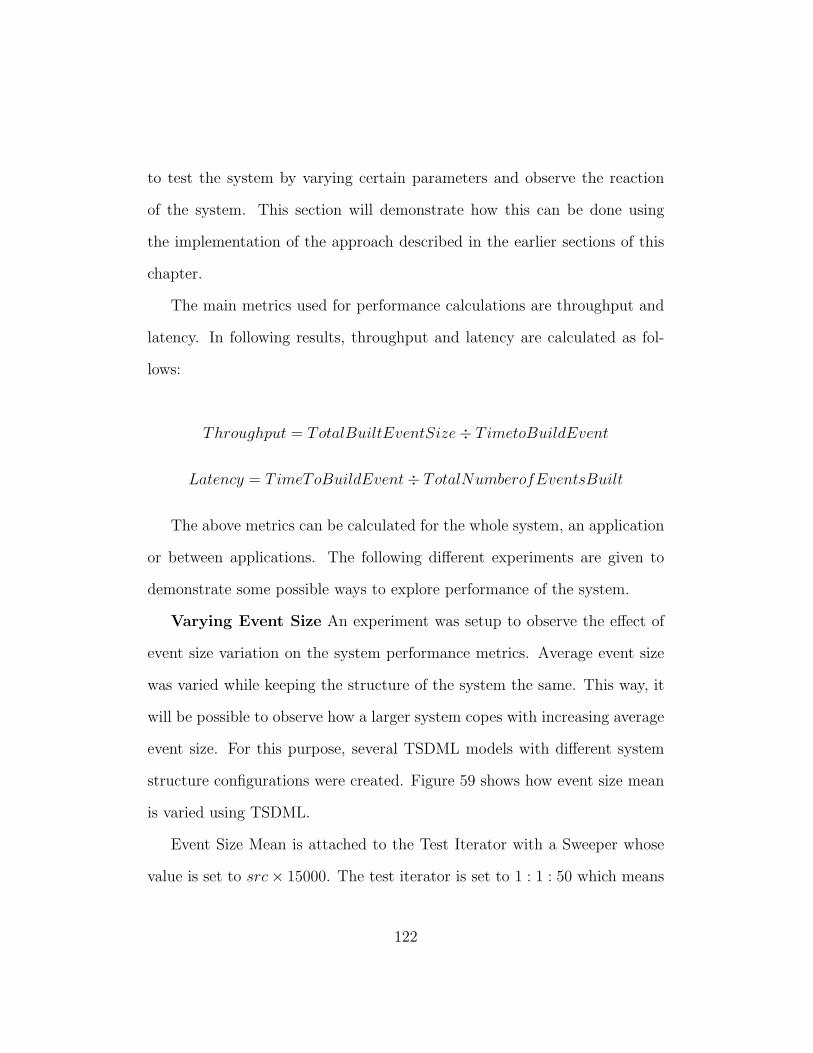
to test the system by varying certain parameters and observe the reaction

of the system. This section will demonstrate how this can be done using

the implementation of the approach described in the earlier sections of this

chapter.

The main metrics used for performance calculations are throughput and

latency. In following results, throughput and latency are calculated as fol-

lows:

Throughput = TotalBuiltEventSize÷ TimetoBuildEvent

Latency = TimeToBuildEvent÷ TotalNumberofEventsBuilt

The above metrics can be calculated for the whole system, an application

or between applications. The following different experiments are given to

demonstrate some possible ways to explore performance of the system.

Varying Event Size An experiment was setup to observe the effect of

event size variation on the system performance metrics. Average event size

was varied while keeping the structure of the system the same. This way, it

will be possible to observe how a larger system copes with increasing average

event size. For this purpose, several TSDML models with different system

structure configurations were created. Figure 59 shows how event size mean

is varied using TSDML.

Event Size Mean is attached to the Test Iterator with a Sweeper whose

value is set to src× 15000. The test iterator is set to 1 : 1 : 50 which means

122

Figure 59: Event Size Variation

there will be 50 test cases. Figure 60 shows the change in event size and,

Figure 61 shows the change in system throughput and latency with respect

to change in event size.

It can be observed from the trends of throughput and latency in Figure 61

that both system throughput and latency is increasing as the size of events

fed into the system are increased. This is expected for throughput because

total event size is increasing by every test case. The increase is also expected

for latency since it is taking more time to build an event while the total

number of events build was held constant.

Figure 61 also shows the effect of increasing the system structure on

throughput and latency. For a 2-by-2 system, system throughput was de-

creased and system latency was increased compared to the 1-by-1 system.

A 2 by 2 system means that there are 2 RUs and 2 BUs that participate in

event building. This trend in throughput and latency means that time to

123

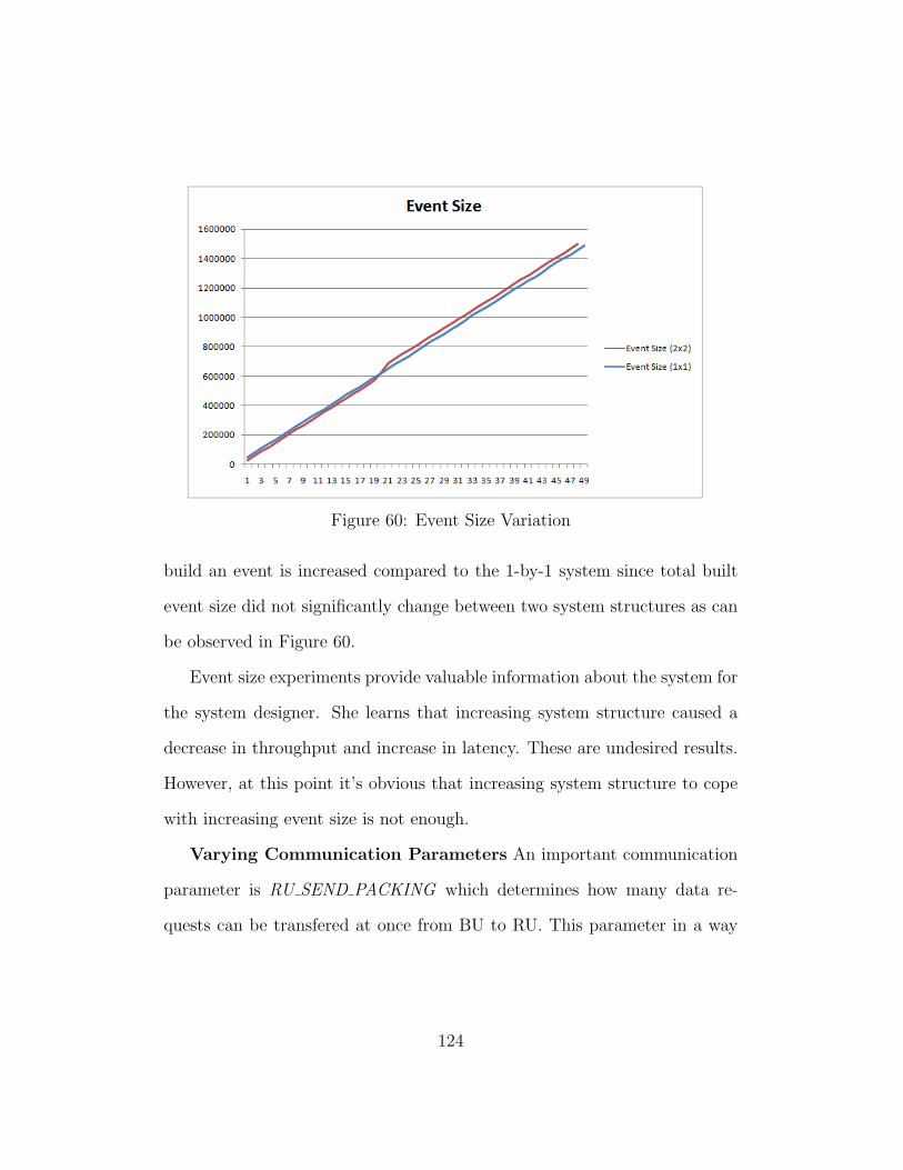
Figure 60: Event Size Variation

build an event is increased compared to the 1-by-1 system since total built

event size did not significantly change between two system structures as can

be observed in Figure 60.

Event size experiments provide valuable information about the system for

the system designer. She learns that increasing system structure caused a

decrease in throughput and increase in latency. These are undesired results.

However, at this point it’s obvious that increasing system structure to cope

with increasing event size is not enough.

Varying Communication Parameters An important communication

parameter is RU SEND PACKING which determines how many data re-

quests can be transfered at once from BU to RU. This parameter in a way

124

Figure 61: Throughput vs Event Size

125

Figure 62: Variation in Number of Events

simulates the bandwidth between BU and RU and has potential effect on per-

formance. In order to observe how RU SEND PACKING parameter would

effect the system, total number of events to be build by the system was var-

ied while keeping the RU SEND PACKING parameter constant. This can

be achieved by using a sweeper to vary number of events fed into the system

in a TSDML model. Several of these models can be created with different

RU SEND PACKING parameter values. For this experiment three different

parameter values were tested. If the experiment is designed this way, test

generation creates several test cases that span all desired configurations.

Figure 62 shows how the number of events were varied for each test and

Figure 63 shows the system throughput and latency for each set of experi-

ment.

126

Figure 63: Throughout and Latency vs Number of Events

127

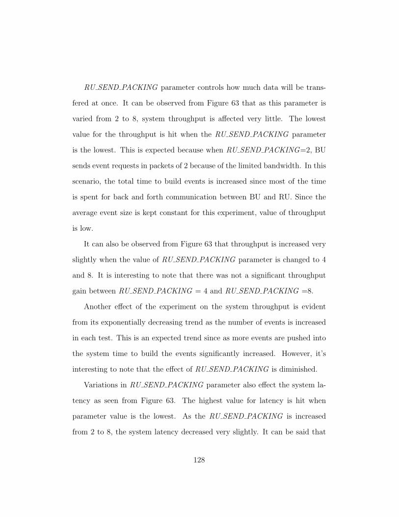
RU SEND PACKING parameter controls how much data will be trans-

fered at once. It can be observed from Figure 63 that as this parameter is

varied from 2 to 8, system throughput is affected very little. The lowest

value for the throughput is hit when the RU SEND PACKING parameter

is the lowest. This is expected because when RU SEND PACKING=2, BU

sends event requests in packets of 2 because of the limited bandwidth. In this

scenario, the total time to build events is increased since most of the time

is spent for back and forth communication between BU and RU. Since the

average event size is kept constant for this experiment, value of throughput

is low.

It can also be observed from Figure 63 that throughput is increased very

slightly when the value of RU SEND PACKING parameter is changed to 4

and 8. It is interesting to note that there was not a significant throughput

gain between RU SEND PACKING = 4 and RU SEND PACKING =8.

Another effect of the experiment on the system throughput is evident

from its exponentially decreasing trend as the number of events is increased

in each test. This is an expected trend since as more events are pushed into

the system time to build the events significantly increased. However, it’s

interesting to note that the effect of RU SEND PACKING is diminished.

Variations in RU SEND PACKING parameter also effect the system la-

tency as seen from Figure 63. The highest value for latency is hit when

parameter value is the lowest. As the RU SEND PACKING is increased

from 2 to 8, the system latency decreased very slightly. It can be said that

128

RU SEND PACKING parameter did not affect system latency in a signifi-

cant way. Latency trend is upwards since total time to build events is in-

creased by each test since the number events were fed into the system is

increased. It is also observed that there was not a significant latency gain

between RU SEND PACKING = 4 and RU SEND PACKING = 8.

RU SEND PACKING parameter plays a role in communication between

BU and RU as stated earlier. For this reason, it may also be interesting

to investigate the change in throughput and latency of BU with respect

to the variations in this parameter. Figure 64 shows BU throughput and

latency for all different values of the RU SEND PACKING parameter. It

can be observed that BU throughput increased as RU SEND PACKING is

increased. On the other hand, BU latency was affected very significantly in

response to the increase in RU SEND PACKING parameter. In addition to

decreasing to very low values, BU latency also shows stabilization against

increasing number of events.

Experiments with RU SEND PACKING parameter provides valuable in-

formation to the system designer. Based on these results, she can choose

to tune the system so that the parameter is set to at least 4. On the other

hand, based on performance requirements, she may choose to experiment in

a similar manner by feeding more events into the system and varying the

parameter value above 8.

129

Figure 64: BU Throughput and Latency

Another communication parameter is RU READOUT PACKING. A sim-

ilar experiment was conducted to see the effect of this parameter on perfor-

mance. Similar results were obtained but as a different observation, it’s

worthwhile to investigate the impact on RU latency. Figure 65. As expected

RU latency is at its highest level when RU READOUT PACKING is lowest.

When RU READOUT PACKING is increased, a significant decrease in RU

latency when RU READOUT PACKING is observed.

Comparison to Related Work

There are many performance analysis and performance testing approaches

in the literature. In this section, a brief discussion on the differences of the

approach described in Chapter II and implemented in this chapter to some

important work in the literature.

130

Figure 65: RU Latency

In [9], Liu and Gorton target the problem of predicting the performance

of a large-scale enterprise system before the implementation of the system.

They use an empirical approach to generate product-specific performance

profiles that help with prediction of performance of middleware technologies

such as CORBA, COM+ and J2EE. They focus on designing a test suite

characterizing the behavior and performance profile of a J2EE application

server product. In their approach, Liu and Gorton focus on testing the mid-

dleware in an isolated manner and do not concentrate on complex interactions

among applications and the middleware. The notion of a test case for Liu

and Gorton is a an application called “identity application” which is a very

basic application that will run on the middleware platform. It is a basic

application whose only methods are read and write which are responsible for

reading and incrementing the value field in a single table relational database,

131

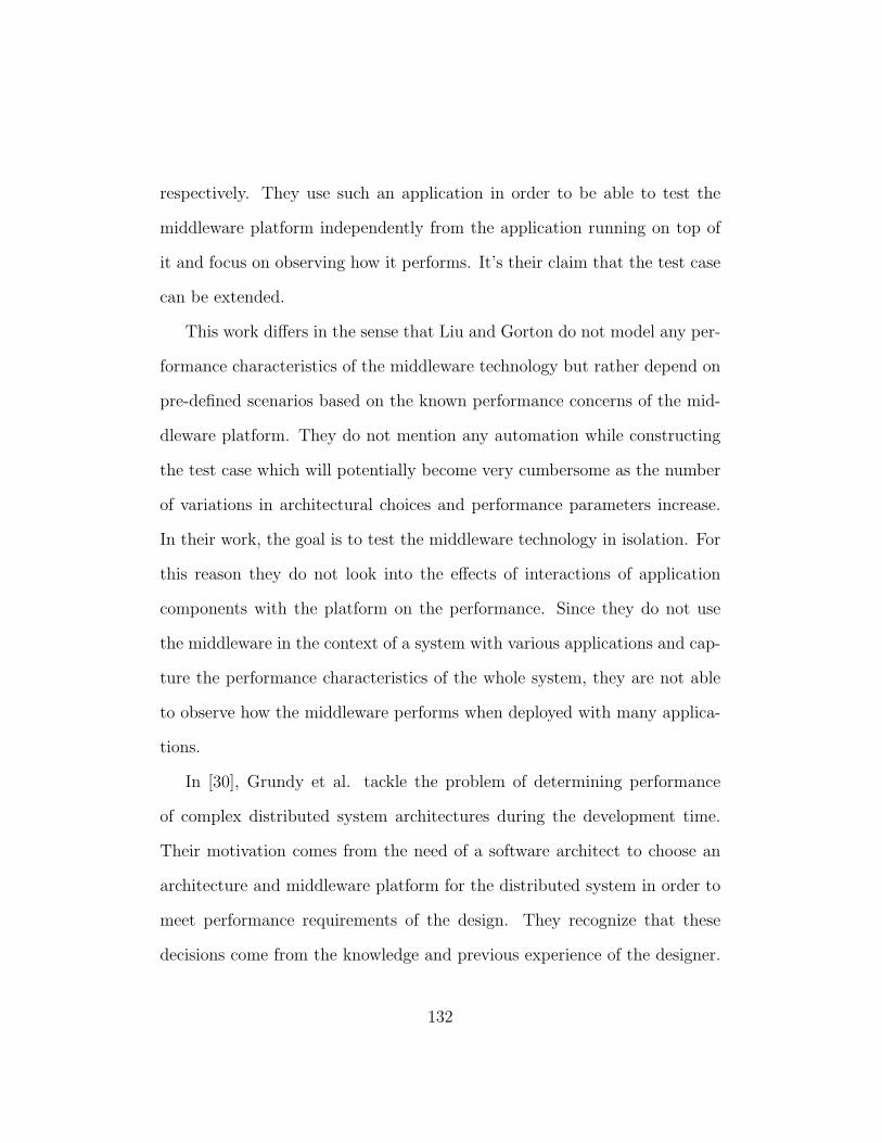
respectively. They use such an application in order to be able to test the

middleware platform independently from the application running on top of

it and focus on observing how it performs. It’s their claim that the test case

can be extended.

This work differs in the sense that Liu and Gorton do not model any per-

formance characteristics of the middleware technology but rather depend on

pre-defined scenarios based on the known performance concerns of the mid-

dleware platform. They do not mention any automation while constructing

the test case which will potentially become very cumbersome as the number

of variations in architectural choices and performance parameters increase.

In their work, the goal is to test the middleware technology in isolation. For

this reason they do not look into the effects of interactions of application

components with the platform on the performance. Since they do not use

the middleware in the context of a system with various applications and cap-

ture the performance characteristics of the whole system, they are not able

to observe how the middleware performs when deployed with many applica-

tions.

In [30], Grundy et al. tackle the problem of determining performance

of complex distributed system architectures during the development time.

Their motivation comes from the need of a software architect to choose an

architecture and middleware platform for the distributed system in order to

meet performance requirements of the design. They recognize that these

decisions come from the knowledge and previous experience of the designer.

132

They present a way and an integrated tool which enables the designer to

sketch a high-level description of the system and generates an executable

test bed which can be deployed on multiple client and server hosts.

In their approach, Grundy et al. model the system at the architectural

level and provide an architecture design modeling language called SoftArch

[30]. The metamodel for SoftArch provides the abstractions to model client,

server, database and host elements along with expected client, server and

database services. Properties such as request quantity and frequency, com-

plexity of database tables are requests, middleware protocol are also specified.

From this high-level descriptions, an executable test code is generated and

uploaded to the host machines.

This approach comes closer to the approach described in this thesis in the

sense that there is a model of the system from the architecture level and test

cases are automatically generated from these models. Grundy et al. mention

that “SoftArch client and server code annotations are usually used to capture

performance measures” but there is not an explicit description of how the

annotations are made and what is captured in those annotations. Moreover,

since their metamodel is from architecture level, the do not capture any data

flow and performance aspects of the system. Furthermore, they do not model

an entire system using the middleware in the architecture they specify. For

this reason, they are not able to determine the effect of interaction between

applications and middleware, and various configurations of applications on

the performance of the system. It is understood for their descriptions that the

133

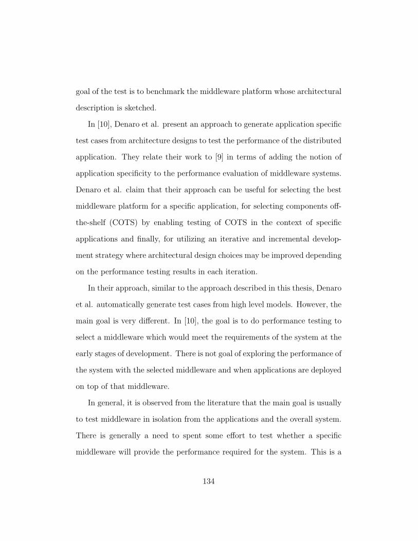
goal of the test is to benchmark the middleware platform whose architectural

description is sketched.

In [10], Denaro et al. present an approach to generate application specific

test cases from architecture designs to test the performance of the distributed

application. They relate their work to [9] in terms of adding the notion of

application specificity to the performance evaluation of middleware systems.

Denaro et al. claim that their approach can be useful for selecting the best

middleware platform for a specific application, for selecting components off-

the-shelf (COTS) by enabling testing of COTS in the context of specific

applications and finally, for utilizing an iterative and incremental develop-

ment strategy where architectural design choices may be improved depending

on the performance testing results in each iteration.

In their approach, similar to the approach described in this thesis, Denaro

et al. automatically generate test cases from high level models. However, the

main goal is very different. In [10], the goal is to do performance testing to

select a middleware which would meet the requirements of the system at the

early stages of development. There is not goal of exploring the performance of

the system with the selected middleware and when applications are deployed

on top of that middleware.

In general, it is observed from the literature that the main goal is usually

to test middleware in isolation from the applications and the overall system.

There is generally a need to spent some effort to test whether a specific

middleware will provide the performance required for the system. This is a

134

valid concern and an area to do performance testing. However, many of the

approaches do not go several steps further and attempt to model a whole

distributed middleware based system from performance perspective and try

to explore the performance of the system based on various performance char-

acteristics of systems components.

Furthermore, in model based performance testing approaches given in

this section, there is a need to model solely from performance point of view.

On the other hand, the approach described in this thesis, approaches mod-

eling the system from a more general model based development perspective

and supplementing the models with performance characteristics of the com-

ponents. If the goal is to just use another middleware to observe how it will

perform, it’s sufficient to plug in the model of that middleware at the de-

sired level of detail to observe the changes in the system performance. Using

this approach, the systems designer does not need to separate the concerns

of functional behavior and performance and is not forced to come up with

a separate performance model at the different level of detail using differ-

ent modeling constructs. Moreover, it’s possible to use this approach from

the beginning phase of development and incrementally improve the structure

and behavior models and never loose track of the performance record of the

system.

Finally, it can be said that the approach described in this thesis, makes an

important contribution with the parameterized (iterators, replicators, con-

nectors and sweepers) and hybrid (structural DSML models, and behavioral

135

DEVS models) modeling and test generation and execution approach intro-

duced.

Summary

In this chapter, implementation of the approach described in Chapter II

was described. Details of the system under test and application simulation

models were presented. It was shown that it’s possible to generate several

test cases from a single TSDML model for the CMS DAQ system.

Performance testing approach presented in this chapter focused on get-

ting performance information from a system during simulation run time and

applying that information to the system during design time. The imple-

mentation allowed investigating the impact of certain system parameters on

the system performance. The goal was not to come up with very realis-

tic performance numbers for the system under test. The goal was rather

to demonstrate that it’s possible to perform performance engineering on a

system using the model based approach described in Chapter II.

136

CHAPTER VI

CONCLUSION AND FUTURE WORK

A model based method to help build a distributed middleware based sys-

tem, capture its performance characteristics and perform performance testing

and/or performance engineering on it was introduced. The method consisted

of creating a domain specific modeling language for capturing the structure

and performance characteristics of the system, and creating a discrete event

based model to capture the behavior of the system. In order to model the

structure and performance aspect of the system, Model Integrated Comput-

ing (MIC) [7] and to model the behavior of the system Open DEVS modeling

formalism was used [2].

The methodology described in this thesis was applied to a high energy

physics system called CMS XDAQ and results from performance tests were

presented. Although the implementation was demonstrated on a physics

system, the method is general for distributed middleware based systems.

One way this is ensured is that the modeling approach consisted of a domain

specific modeling language for the domain of distributed middleware based

systems. As a part of this domain specific modeling language, modeling

constructs that are common to general set of distributed middleware based

systems. For example, all systems in this domain involve data flow and

deployment considerations and generic constructs for modeling such aspects

of the domain are provided. Furthermore, the domain specific modeling

137

language, called Test Series Definition Modeling Language, is not coupled

with the physics system that the implementation was demonstrated on.

Moreover, for modeling behavior of the system, the modeling and analysis

formalism for discrete event systems called Discrete Event System Specifi-

cation (DEVS) was used. Systems in the domain of distributed middleware

based systems can be described using this formalism independent of the im-

plementation described in this thesis.

Future Work

The approach described in this thesis can be improved in the future in

various ways. One obvious improvement would be to add more detail to the

domain specific modeling language to capture more details of the system.

For example, for the data flow aspect of the system, more details about the

networking aspect of application communication can be captured connections

between objects can be moved to different network lines. Similarly, a detailed

network switching system can be modeled to distribute the data coming in

to the system to different applications.

An interesting improvement can be made in the test design cycle of the

process. Even though the process of generating test cases are automated,

and a generative modeling approach is used to iterate over and replicate

certain elements of the system is possible, design of the actual experiment

is a manual effort. This effort requires deep knowledge of the system to be

138

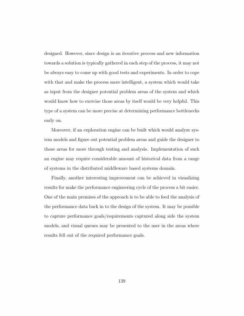
designed. However, since design is an iterative process and new information

towards a solution is typically gathered in each step of the process, it may not

be always easy to come up with good tests and experiments. In order to cope

with that and make the process more intelligent, a system which would take

as input from the designer potential problem areas of the system and which

would know how to exercise those areas by itself would be very helpful. This

type of a system can be more precise at determining performance bottlenecks

early on.

Moreover, if an exploration engine can be built which would analyze sys-

tem models and figure out potential problem areas and guide the designer to

those areas for more through testing and analysis. Implementation of such

an engine may require considerable amount of historical data from a range

of systems in the distributed middleware based systems domain.

Finally, another interesting improvement can be achieved in visualizing

results for make the performance engineering cycle of the process a bit easier.

One of the main premises of the approach is to be able to feed the analysis of

the performance data back in to the design of the system. It may be possible

to capture performance goals/requirements captured along side the system

models, and visual queues may be presented to the user in the areas where

results fell out of the required performance goals.

139

BIBLIOGRAPHY

[1] Philip A. Bernstein. Middleware an architecture for distributed systemservices. Communications of the ACM, 39:86–98, 1993.

[2] Devspp:c++ open source library of devs formalism,http://odevspp.sourceforge.net/.

[3] IEEE Std 610.12-1990. IEEE standard glossary of software engineeringterminology. 1990.

[4] E.J. Weyuker and F.I. Vokolos. Experience with performance testing ofsoftware systems: Issues, an approach and case study. Software Engi-neering, IEEE Transactions on, 26.

[5] Richard E. Schantz and Douglas C. Schmidt. Middleware for distributedsystems - evolving the common structure for network-centric applica-tions, July 30 2001.

[6] Jerry Zeyu Gao, H.-S. Jacob Tsao, and Ye Wu. Testing and QualityAssurance for Component-Based Software. Artech House Publishers,September 2003.

[7] Janos Sztipanovits and Gabor Karsai. Model-integrated computing.IEEE Computer, 30:110–112, April 1997.

[8] Bernard P. Zeigler. Theory of Modelling and Simulation. Krieger Pub-lishing Co., Inc., Melbourne, FL, USA, 1984.

[9] Yan Liu, Ian Gorton, Anna Liu, Ning Jiang, and Shiping Chen. Design-ing a test suite for empirically-based middleware performance prediction.In CRPIT ’02: Proceedings of the Fortieth International Conference onTools Pacific, pages 123–130, Darlinghurst, Australia, Australia, 2002.Australian Computer Society, Inc.

[10] Giovanni Denaro, Andrea Polini, and Wolfgang Emmerich. Early per-formance testing of distributed software applications. SIGSOFT Softw.Eng. Notes, 29(1):94–103, 2004.

140

[11] G. Denaro, A. Polini, and W. Emmerich. Performance testing of dis-tributed component architectures. Springer, 2005.

[12] Turker Keskinpala. Model based perofmrnace testing of distributed largescale systems. Area Paper, October 2006.

[13] Jack Greenfield, Keith Short, Steve Cook, and Stuart Kent. SoftwareFactories: Assembling Applications with Patterns, Models, Frameworks,and Tools. Wiley, August 2004.

[14] Akos Ledeczi, Miklos Maroti, Arpad Bakay, Greg Nordstrom, Jason Gar-rett, Chuck Thomasson, Jonathan Sprinkle, and Peter Volgyesi. Gme2000 users manual (v2.0), December 2001.

[15] Gme manual and user guide, version 7.0.

[16] A. Ledeczi, A. Bakay, M. Maroti, P. Volgyesi, G. Nordstrom, J. Sprin-kle, and G. Karsai. Composing domain-specific design environments.Computer, 34(11):44–51, 2001.

[17] Lawrence Chung, Brian A. Nixon, Eric Yu, and John Mylopoulos. Non-Functional Requirements in Software Engineering (THE KLUWER IN-TERNATIONAL SERIES IN SOFTWARE ENGINEERING Volume 5)(International Series in Software Engineering). Springer, October 1999.

[18] Connie U. Smith. Performance Engineering of Software Systems.Addison-Wesley Longman Publishing Co., Inc., Boston, MA, USA, 1990.

[19] C. U. Smith and L. G. Williams. Software performance engineering: Acase study including performance comparison with design alternatives.IEEE Trans. Softw. Eng., 19(7):720–741, 1993.

[20] R. Jain. The art of computer systems performance analysis: techniquesfor experimental design, measurement, simulation, and modeling. JohnWiley & Sons, Inc., New York, NY, USA, 1991.

[21] Simonetta Balsamo, Antinisca Di Marco, Paola Inverardi, and MartaSimeoni. Model-based performance prediction in software development:A survey. IEEE Transactions on Software Engineering, 30(5):295–310,2004.

141

[22] Rob Pooley. Software engineering and performance: a road-map. InICSE - Future of SE Track, pages 189–199, 2000.

[23] Dorina C. Petriu and Xin Wang. From uml descriptions of high-levelsoftware architectures to lqn performance models. In AGTIVE ’99:Proceedings of the International Workshop on Applications of GraphTransformations with Industrial Relevance, pages 47–62, London, UK,2000. Springer-Verlag.

[24] Steve J. H. Yang Ross A. W. Smith Jeffrey J. P. Tsai, Yaodong Bi.Distributed Real-Time Systems: Monitoring, Visualization, Debugging,and Analysis. Wiley-Interscience, July 1996.

[25] B. Beizer and J. Wiley. Black box testing: Techniques for functionaltesting of software and systems. IEEE Software, 13(5), 1996.

[26] Cms technical design report: Data acquisition and high-level trigger,December 2002.

[27] J. Gutleber, E. Cano, S. Cittolin, F. Meijers, L. Orsini, and D. Samyn.Architectural software support for processing clusters. 2000.

[28] Ru builder user manual.

[29] Boost c++ libraries, http://www.boost.org/.

[30] John C. Grundy, Yuhong Cai, and Anna Liu. Softarch/MTE: Gener-ating distributed system test-beds from high-level software architecturedescriptions. Autom. Softw. Eng, 12(1):5–39, 2001.

142