Model-Based Geostatistics for Prevalence Mapping in

Low-Resource Settings

Peter J Diggle and Emanuele Giorgi

(Lancaster Medical School, Lancaster University)

December 18, 2015

Abstract

In low-resource settings, prevalence mapping relies on empirical prevalence data from

a finite, often spatially sparse, set of surveys of communities within the region of interest,

possibly supplemented by remotely sensed images that can act as proxies for environ-

mental risk factors. A standard geostatistical model for data of this kind is a generalized

linear mixed model with binomial error distribution, logistic link and a combination of

explanatory variables and a Gaussian spatial stochastic process in the linear predictor.

In this paper, we first review statistical methods and software associated with this stan-

dard model, then consider several methodological extensions whose development has

been motivated by the requirements of specific applications. These include: methods for

combining randomised survey data with data from non-randomised, and therefore po-

tentially biased, surveys; spatio-temporal extensions; spatially structured zero-inflation.

Throughout, we illustrate the methods with disease mapping applications that have

arisen through our involvement with a range of African public health programmes.

Keywords: geostatistics; multiple surveys; prevalence; spatio-temporal models; zero-

inflation.

1

1 Introduction

The term “geostatistics” is typically used as a convenient shorthand for statistical models

and methods associated with analysing spatially discrete data relating to an unobserved spa-

tially continuous phenomenon. The name derives from its origins in the South African mining

industry (Krige, 1951) and its subsequent development by the late Georges Matheron and

colleagues in L’Ecole des Mines, Fontainebleau, France (Chiles & Delfiner, 2012). Geostatis-

tical methodology has since been applied in a wide range of scientific contexts, and is now

widely accepted as one of three main branches of spatial statistics (Cressie, 1993). The de-

scriptive phrase “model-based geostatistics” was coined by Diggle, Tawn & Moyeed (1998)

to mean the embedding of geostatistics within the general framework of statistical modelling

and likelihood-based inference as applied to geostatistical problems. In contrast, “classical”

Fontainebleau-style geostatistics has its own terminology and self-contained methodology, de-

veloped largely independently of the statistical mainstream.

Whether tackled through the model-based or classical approach, a typical feature of most

geostatistical problems is a focus on prediction rather than on parameter estimation. The

canonical geostatistical problem, expressed in the language of model-based geostatistics, is the

following. Data {(yi, xi) : i = 1, ..., n} are realised values of random variables Yi associated

with pre-specified locations xi ∈ A ⊂ IR2. The Yi are assumed to be statistically dependent

on an unobserved stochastic process, S = {S(x) : x ∈ IR2}, as expressed through a statistical

model [S, Y ] = [S][Y |S], where [·] means “the distribution of,” Y = (Y1, ..., Yn) and S =

{S(x1), ..., S(xn)}. What can be said about the realisation of S? The formal model-based

solution is the conditional distribution, [S|Y ] = [S|S][S|Y ], where [S|Y ] follows as a direct

application of Bayes’ theorem,

[S|Y ] = [S][Y |S]/

∫[S][Y |S]dS.

2

By far the most tractable case is the linear Gaussian model, for which S is a Gaussian process

and the Yi given S are conditionally independent, Yi|S ∼ N(S(xi), τ2). It follows that the

marginal distribution of Y , the conditional distribution [S|Y ] and the conditional distribution

[S|S] are all multivariate Normal.

Note that in the above formulation, no model is specified for the xi. We return to this

point in the discussion, but in the meantime the implicit assumption is that the xi are pre-

specified as part of the study-design or are located according to a process that is stochastically

independent of S. If X = (x1, ..., xn) is stochastic, a complete factorisation of the model for

the data is [S,X, Y ] = [S][X|S][Y |X,S]. Then, if [X|S] = [X] and the properties of [X] are

not of interest, it is legitimate to condition on [X] and so recover the previous formulation,

[S, Y ] = [S][Y |S].

Diggle, Moraga, Rowlingson & Taylor (2013) argue that the geostatistical label should be

applied more generally to scientific problems that involve predictive inference about an un-

observed spatial phenomenon S(x) using any form of incomplete information. This includes,

for example, predictive inference for the intensity of a Cox process (Cox, 1955), and inference

when X is both stochastic and dependent on S.

In this paper, we restrict our substantive scope to the problem of analysing data from spatially

referenced prevalence surveys. We also focus on prevalence mapping in low-resource countries

where registry data are lacking. We argue that in low-resource settings the sparsity of the

available data justifies a more strongly model-based approach than would be appropriate if

accurate registries were available.

2 The standard geostatistical model for prevalence data

In its most basic form, a prevalence survey consists of visiting communities at locations xi :

i = 1, ..., n distributed over a region of interest A and, in each community, sampling mi

3

individuals and recording whether each tests positive or negative for the disease of interest.

If p(x) denotes prevalence at location x, the standard sampling model for the resulting data

is binomial, Yi ∼ Bin(mi, p(xi)) for i = 1, ..., n. Linkage of the p(xi) at different locations

is usually desirable, and is essential if we wish to make inferences about p(x) at unsampled

locations x.

The simplest extension to the basic model is a binary regression model, for example a logistic

regression model of the form

log[p(xi)/{1− p(xi)}] = d(xi)′β, (1)

where d(xi) is a vector of explanatory variables associated with the location xi. This assumes

that the value of d(x) is available not only at the data-locations xi but also at any other

location x that is of interest. When extra-binomial variation is present, two further extensions

are possible. Firstly, a standard mixed effects model adds a random effect to the right-hand-

side of (1), to give

log[p(xi)/{1− p(xi)}] = d(xi)′β + Zi,

where the Zi are independent N(0, τ 2) variates. Secondly, if the context suggests that covariate-

adjusted prevalence should vary smoothly over the region of interest, we can add a spatially

correlated random effect, to give

log[p(xi)/{1− p(xi)}] = d(xi)′β + S(xi) + Zi, (2)

where S = {S(x) : x ∈ IR2} is a Gaussian process with mean zero, variance σ2 and correlation

function ρ(x, x′) = Corr{S(x), S(x′)}. We shall assume that the process S is stationary and

isotropic, hence Corr{S(x), S(x′)} = ρ(||x− x′||), where || · || denotes the Euclidean distance.

Amongst the various parametric families that have been proposed for ρ(u), Stein (1999) ad-

4

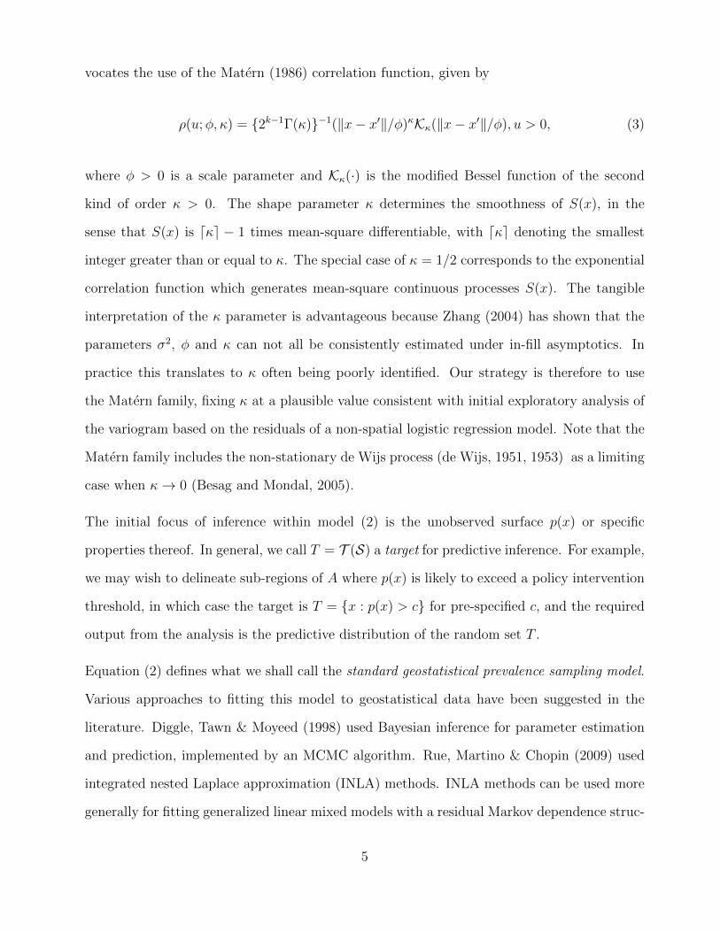
vocates the use of the Matern (1986) correlation function, given by

ρ(u;φ, κ) = {2k−1Γ(κ)}−1(‖x− x′‖/φ)κKκ(‖x− x′‖/φ), u > 0, (3)

where φ > 0 is a scale parameter and Kκ(·) is the modified Bessel function of the second

kind of order κ > 0. The shape parameter κ determines the smoothness of S(x), in the

sense that S(x) is dκe − 1 times mean-square differentiable, with dκe denoting the smallest

integer greater than or equal to κ. The special case of κ = 1/2 corresponds to the exponential

correlation function which generates mean-square continuous processes S(x). The tangible

interpretation of the κ parameter is advantageous because Zhang (2004) has shown that the

parameters σ2, φ and κ can not all be consistently estimated under in-fill asymptotics. In

practice this translates to κ often being poorly identified. Our strategy is therefore to use

the Matern family, fixing κ at a plausible value consistent with initial exploratory analysis of

the variogram based on the residuals of a non-spatial logistic regression model. Note that the

Matern family includes the non-stationary de Wijs process (de Wijs, 1951, 1953) as a limiting

case when κ→ 0 (Besag and Mondal, 2005).

The initial focus of inference within model (2) is the unobserved surface p(x) or specific

properties thereof. In general, we call T = T (S) a target for predictive inference. For example,

we may wish to delineate sub-regions of A where p(x) is likely to exceed a policy intervention

threshold, in which case the target is T = {x : p(x) > c} for pre-specified c, and the required

output from the analysis is the predictive distribution of the random set T .

Equation (2) defines what we shall call the standard geostatistical prevalence sampling model.

Various approaches to fitting this model to geostatistical data have been suggested in the

literature. Diggle, Tawn & Moyeed (1998) used Bayesian inference for parameter estimation

and prediction, implemented by an MCMC algorithm. Rue, Martino & Chopin (2009) used

integrated nested Laplace approximation (INLA) methods. INLA methods can be used more

generally for fitting generalized linear mixed models with a residual Markov dependence struc-

5

ture. Also, Lindgren, Rue & Lindstrm (2011) has shown that random field models can be

expressed as solutions to continuous domain stochastic partial differential equations (SPDEs).

This gives an explicit link between the parameters of each SPDE and the elements of the cor-

responding precision matrix in a spatially discrete basis-function representation. The practical

consequence of this is that INLA can be used for approximate inference on spatially contin-

uous Gaussian random fields using computationally fast methods based on spatially discrete

Markov random fields. The INLA methodology and its associated software yield accurate and

computationally fast approximations to the marginal posterior distributions of model param-

eters and to the marginal predictive distribution of S(x) at each element of a set of locations

x, but not to their joint predictive distribution. This limits INLA’s applicability to point-wise

targets T , whereas in many applications the targets T involves the complete process S or,

in practice, its restriction to a fine grid of locations to cover the region of interest; examples

include area-wide summaries of S(x), such as its spatial average or the proportion over a

specified threshold. In the application of Section 5, we give an example where the target is

the village-level average of malaria prevalence.

Giorgi & Diggle (2014) provide an R package for Monte Carlo maximum likelihood estima-

tion and plug-in prediction with an option to use a low-rank approximation to S for faster

computation with large data-sets. The low-rank method approximates S by S∗, where

S∗(x) =r∑

k=1

f(x− xk)Vk. (4)

In (4), the Vk are independent N(0, τ 2) variates associated with a pre-specified set of locations

xk and f(x) is a prescribed function, typically monotone non-increasing in ||x||. The covariance

function of S∗ is

Cov{S∗(x), S∗(x′)} = τ 2r∑

k=1

f(x− xk)f(x′ − xk), (5)

Low-rank specifications have been proposed as models in their right; see, for example, Higdon

(1998, 2002). We consider them as approximations to a limiting, full-rank process. Taking

6

the xk in (4) as the points of an increasingly fine regular lattice and scaling the function

f(·) commensurate with the lattice spacing gives a limiting, full-rank process with covariance

function

Cov{S∗(x), S∗(x′)} = τ 2∫

IR2f(x− u)f(x′ − u)du. (6)

From this perspective, the summation in (5) represents a quadrature approximation to the

integral in (6). As the scale of the spatial correlation increases, a smaller number of xk points

is required for an adequate approximation. In practice, we start with a computationally

convenient value for r which we then increase until the spatial predictions for a specific target

stabilise; Giorgi & Diggle (2014) give an example on a simulated data-set.

Gotway & Stroup (1997) suggest using generalized estimating equations (Liang & Zeger, 1986)

when scientific interest is focused on the regression parameters rather than on prediction of S.

However, in this approach the implicit target for inference is not the parameter vector β that

appears in (2), but rather the marginal regression parameter vector, β∗ say. The elements of

β∗ are smaller in absolute value than those of β by an amount that depends on τ 2, σ2 and

ρ(u).

Diggle et al. (2007) use the standard model (2), but without the mutually independent random

effects Zi, to construct predictive maps of the prevalence of Loa loa, a parasitic infection of

the eye, in an area of equatorial west Africa covering Cameroon and parts of its neighbouring

countries. Following Thomson et al. (2004) they include two remotely sensed covariates,

height above sea-level and the Normalised Digital Vegetation Index (NDVI), as proxies for

the ability of the disease vector, a particular species of Chrysops fly, to breed at each location.

As described in Thomson et al. (2004) and Diggle et al. (2007), Loa loa prevalence mapping

plays an important role in the implementation of a multi-national prophylactic mass-treatment

programme for the control of onchocerciasis (river blindness), the African Programme for

Onchocerciasis Control, APOC (WHO, 2012), following the recognition that a generally safe

filaricide medication, Ivermectin, could produce severe, occasionally fatal, adverse reactions

7

Figure 1: Predictive probability map of Loa loa prevalence in Cameroon and surroundingareas (adapted from Diggle et al. (2007)). Empirical prevalences at surveyed locations areindicated by size and colour coded dots.

in people heavily co-infected with onchocerciasis and Loa loa parasites. As a result, APOC

adopted the policy that in areas where Loa loa prevalence was greater than 20%, precautionary

measures should be taken before local administration of Ivermectin.

Diggle et al. (2007) mapped the minimum mean square error point predictor, E[p(x)|y] but

also argued that a more useful quantity was the point-wise predictive probability, q(x) say,

that p(x) exceeded 0.2, in line with APOC’s precautionary policy. In addition to addressing

directly the relevant practical problem, a map of q(x) conveys the uncertainty associated with

the resulting predictions. This map, here reproduced as Figure 1, identifies large areas that

almost certainly do and do not meet the policy-intervention criterion, but also delineates

large areas where the only honest answer is “don’t know,” indicating the need for further

investigation or, if practicalities dictate, taking an informed risk.

Other prevalence mapping applications of model-based geostatistics include: Claridge et al.

(2012) on liver fluke and bovine tuberculosis in the UK cattle herd; Clements et al. (2006)

on schistosomiasis in Tanzania; Diggle et al. (2002) on childhood malaria in the Gambia;

8

Gemperli et al. (2004) on infant mortality in Mali; Gething et al. (2012) on the world-wide

distribution of Plasmodium vivax; Hay et al. (2009) on the world-wide distribution of Plasmod-

ium falciparium; Kleinschmidt et al. (2001) on malaria incidence in Kwazuku Natal, South

Africa; Kleinschmidt et al. (2007) on HIV in South Africa; Soares Magalhaes & Clements

(2011) on anemia in preschool-aged children in West Africa; Raso et al. (2005) on schistoso-

miasis in Cote D’Ivoire; Pullan et al. (2011) on soil-transmitted infections in Kenya; Zoure

et al. (2014) on river blindness in the 20 participating countries of the African Programme for

Onchocerciasis control.

3 Computational details

In each of the applications to be described in Section 4 to 6, we use the Monte Carlo maximum

likelihood (MCML) method for parameter estimation. This fitting procedure can be used

under a very general modelling framework. Let Wi for i = 1, . . . , n denote a set of random

effects associated with Yi, following a joint multivariate Normal distribution with mean µ

and covariance matrix Σ. Assume that Yi conditionally on Wi are mutually independent

random variables with distributions f(·|Wi). The likelihood function for the vector of model

parameters θ is given by

L(θ) =

∫Rdim(W)

g(W, y; θ) dW

=

∫Rdim(W)

N(W ;µ,Σ)n∏i

f(yi|Wi) dW,

where dim(W ) denotes the dimension of W . Note, for example, that in the model used

in Section 6.1, the random effect associated with village i is a bivariate random variable,

Wi = {S(xi) + Zi, T (xi)}, hence dim(W ) = 2n with f(·|Wi) given by (14). Monte Carlo

methods are then used in order to approximate the above intractable integral using importance

sampling. As discussed in Giorgi & Diggle (2014), a convenient choice for the importance

9

sampling distribution is g(W, y; θ0) for some fixed θ0, which can be iteratively updated. With

this choice, a Markov chain Monte Carlo (MCMC) algorithm is then required for simulation

of Wi conditionally on yi under θ0. We use a Langevin-Hastings algorithm that updates the

transformed vector of random effects Σ−1/2(W − W ), where W and Σ are the mode and the

inverse of the negative Hessian at W of g(W, y; θ0).

4 Combining information from multiple surveys

In order to obtain good geographical coverage of the population of interest, it is often necessary

to combine information from multiple prevalence surveys. However, understanding the limita-

tions of the sampling design adopted in each survey is crucial in order to draw valid inferences

from a joint analysis of the data. In particular, non-randomized “convenience” surveys in

which data are gathered opportunistically, for example at schools, markets or hospital clinics,

may reach an unrepresentative sub-population or be biased in other ways. Nonetheless, con-

venience samples represent a tempting, low-cost alternative to random samples. A combined

analysis of data from randomised and convenience samples that estimates and adjusts for bias

can be more efficient than an analysis that considers only the data from randomised surveys.

In a non-spatial context, Hedt & Pagano (2011) propose a hybrid estimator of prevalence that

supplements information from random samples with convenience samples, and show that this

leads to more accurate prevalence estimates than those available from using only the data

from randomised surveys.

Giorgi et al. (2015) develop a multivariate generalized linear geostatistical model to account

for data-quality variation amongst spatially referenced prevalence surveys. They assume that

at least one of the available surveys is a “gold-standard” that delivers unbiased prevalence

estimates and for which the standard model (2) is appropriate. Bias in a “non gold-standard”

survey is then modelled using covariate information together with an additional, zero-mean

10

stationary Gaussian process B = {B(x) : x ∈ IR2}. The resulting model for a non-randomised

survey is

log[p(xi)/{1− p(xi)}] = d(xi)′β + S(xi) + Zi + {d(xi)

′δ +B(xi)}. (7)

Data from both the randomised and the non-randomised survey then contribute to inference

on the predictive target, d(x)′β + S(x).

4.1 Application: using school and community surveys to estimate

malaria prevalence in Nyanza Province, Kenya

We now show an application to malaria prevalence data from a community survey and a

school survey conducted in July 2010 in Rachuonyo South and Kisii Central Districts, Nyanza

Province, Kenya. In the community survey, all residents above the age of 6 months were

eligible for inclusion. A finger-prick blood sample was collected on each participant and

examined for presence/absence of malaria parasites by a rapid diagnostic test (RDT).

In the school survey, 46 out of 122 schools with at least 100 pupils were randomly selected using

an iterative process to limit the probability of selecting school with overlapping catchment

areas. All eligible children in attendance were included. In the community survey, residential

compounds lying within 600 meters of each school were randomly sampled and all eligible

residents in each sampled compound examined by the RDT. The design of the community

survey delivers an unbiased sample of residents from the catchment area of each school, whereas

the school survey is potentially biased by a plausible association between a child’s health

status and their attendance at school. More details on the survey procedures can be found in

Stevenson et al. (2013).

In our analysis, we extracted information on sampled individuals between the ages of 6 and 25

years in both surveys, as some adults have taken advantage of the introduction of free primary

education in Kenya. The community survey included 1430 individuals distributed over 740

11

compounds whilst the school survey included 4852 pupils distributed over 3791 compounds,

i.e. averages per compound of approximately 1.9 and 1.3 people, respectively. Figure 2 shows

the locations of the sampled compounds from both surveys.

For our joint analysis of the data from both surveys, we used exponential correlation func-

tions for both S(x) and B(x), with φ and ψ denoting the respective scale parameters. We

parameterise the respective variances of S(x), B(x) and Zi as σ2, ν2σ2 and ω2σ2.

For selection of significant explanatory variables we used ordinary logistic regression, retaining

variables with nominal p-values smaller than 5%. Table 1 gives the final set of explanatory

variables included in the geostatistical model. The “District” indicator variable accounts for

a known higher level of malaria risk in Rachuonoyo district. Socio-economic status (SES) is

an indicator of household wealth taking discrete values from 1 (poor) to 5 (wealthy).

Table 2 reports Monte Carlo maximum likelihood estimates and 95% confidence intervals

for the model parameters. The β-parameters reflect the district effect mentioned above as

well as confirming a lower risk of malaria associated with higher scores of SES and greater

age. The negative estimate of δ0 and its associated confidence interval indicate a significantly

lower malaria prevalence in individuals attending school than in the community at large.

The positive estimate and associated confidence interval for δ1 indicate that for individuals

attending school, the negative effect of age is less strong than in the community. Figure

3(a) shows point-wise predictions of B∗(x) = exp{B(x)}, which represents the unexplained

multiplicative spatial bias in the school survey for the odds of malaria at location x. Figure

3(b) maps the predictive probability, r(x) say, that B∗(x) lies outside the interval (0.9, 1.1),

r(x) = 1− P (0.9 < B∗(x) < 1.1|y) . (8)

The lowest value of r(x) is about 87%, indicating the presence of non-negligible spatially

structured bias throughout the study area. The joint analysis of the data from both surveys

allows us to remove the bias and so obtain more accurate predictions for S(x) than would be

12

Table 1: Explanatory variables used in the analysis of the Kenya malaria prevalence data.

Termβ0 Interceptβ1 Age in yearsβ2 District (=1 if “Rachuonyo”; =0 otherwise)β3 Socio-economic status (score from 1 to 5)δ0 Survey indicator, 1 if “school,” 0 if “community” (bias term)δ1 Age in years (bias term)

Table 2: Monte Carlo maximum likelihood estimates and corresponding 95% confidence in-tervals for the model fitted to the Kenya malaria prevalence data

Estimate 95% Confidence intervalβ0 -1.412 (-2.303, -0.521)β1 -0.141 (-0.174, -0.109)β2 2.006 (1.228, 2.785)β3 -0.121 (-0.169, -0.072)δ0 -0.761 (-1.354, -0.167)δ1 0.094 (0.046, 0.142)

log(σ2) 0.519 (0.048, 0.990)log(ν2) -1.264 (-1.738, -0.790)log(φ) -3.574 (-4.083, -3.064)log(ω2) -1.408 (-2.267, -0.550)log(ψ) -3.366 (-4.178, -2.553)

obtained using only the data from the community survey. Figure 4(a) shows a scatter plot

of the standard errors for S(x) obtained from the joint model for the school and community

surveys and from the model fitted to the community data only. Figure 4(b) shows that

locations for which the joint analysis produces a larger standard errors for S(x) correspond

to areas where no observations were made.

13

34.70 34.75 34.80 34.85 34.90 34.95 35.00

-0.55

-0.50

-0.45

-0.40

Longitude

Latitude

Figure 2: Geographical coordinates of the sampled compounds in the community (black dots)and school (grey traingles) surveys.

14

34.70 34.80 34.90 35.00

-0.55

-0.45

(a)

Longitude

Latitude

0.20.30.40.50.60.70.8

34.70 34.80 34.90 35.00

-0.55

-0.45

(b)

Longitude

Latitude

0.880.900.920.940.960.981.00

Figure 3: The predicted surfaces for B∗(x) (a) and r(x) (b).

15

0.4 0.6 0.8 1.0

0.4

0.6

0.8

1.0

1.2

(a)

Std. errors (community)

Std

. err

ors

(com

mun

ity +

sch

ool)

34.70 34.80 34.90 35.00

-0.60-0.55-0.50-0.45-0.40-0.35

(b)

Longitude

Latitude

Figure 4: (a) Scatterplot of the standard errors for S(x) using data from the communitysurvey only (x-axis) and using both community and school survey data. Points coloured blackor grey lie below or above the identity line y = x, respectively. (b) Prediction locations,coloured black or grey at locations where the prediction variance for S(x) is smaller or larger,respectively, when using the data from both the community and school surveys.

16

5 Analysing spatio-temporally referenced prevalence sur-

veys

In endemic disease settings where prevalence varies smoothly over time, joint analysis of data

from surveys collected at different times can also bring gains in efficiency. The modelling

framework in Giorgi et al. (2015) accommodates multiple surveys conducted at different,

discrete times. The extension of (7) to m surveys conducted at possibly different times is

log[pk(xi)/{1− pk(xi)}] = d(xik)′β + Sk(xi) + Zik +

I(k ∈ B){d(xik)′δ +Bk(xi)}, k = 1, ...,m (9)

where B denotes the indices of the non-randomised surveys, Cov{Sk(x), S ′k(x′)} = σ2αkk′ρ(x, x′)

and αkk′ = 1 if surveys k and k′ are taken at the same time, −1 < αkk′ < 1 otherwise.

A different design for monitoring endemic disease prevalence is the rolling indicator survey

(Roca-Feltrer et al., 2012). This consists of sampling members of a target population of

individuals or households more or less continuously over time, the order of sampling being

randomised. A natural model for the resulting data is a spatio-temporal version of (2),

log[p(xi, ti)/{1− p(xi, ti)}] = d(xi, ti)′β + S(xi, ti) + Zi, (10)

where now (xi, ti) denotes the location and time of the ith sample member. There is an exten-

sive literature on ways of specifying the covariance structure of a spatio-temporal Gaussian

process; see, for example, Gneiting & Guttorp (2010). For endemic diseases, a reasonable

working assumption is that the relative risk of disease at different times is the same at all

locations, and vice versa. This implies an additive formulation,

S(x, t) = S(x) + U(t), (11)

17

where S(x) and U(t) are independent spatial and temporal Gaussian processes, respectively.

5.1 Application: rolling malaria indicator survey in Chikwawa dis-

trict, Malawi, May 2010 to June 2013

We now analyse data from a rolling malaria indicator survey (rMIS) conducted in Chikwawa

District, Southern Malawi, from May 2010 to June 2013. In this rMIS, children under five

years were randomly selected in 50 villages covering an area of approximately 400 km2. Blood

samples were then collected and tested by RDT for malaria. The objectives of the analysis

are the following.

(i) interpolation of the spatio-temporal pattern of malaria prevalence for children under

twelve months;

(i) estimation of the reduction in prevalence and number of infected children through a

scale-up in the distribution of insecticide treated nets (ITN) and delivery of indoor

residual spraying (IRS), from the actual coverage to 100% coverage in each village.

A practical distinction between these two objectives is that the first can only use explanatory

variables that are available throughout the study-region, whereas the second can additionally

use explanatory variables associated with the sampled households.

5.1.1 Spatio-temporal interpolation of malaria prevalence

Let pj(xi, ti) denote the probability of having a positive RDT outcome for the j-th children in

the i-th household at time ti. Using the model defined by (10), the linear predictor assumes

18

the form

log[pj(xi, ti)/{1− pj(xi, ti)}] = β0 + β1dij + β2ti + β3 cos(2πti/12) + β4 sin(2πti/12) +

β5 cos(2πti/6) + β6 sin(2πti/6) + S(xi) + U(ti), (12)

where dij is a binary indicator that takes value 1 if the child is under twelve months and 0

otherwise. The linear combination of sine and cosine functions with periodicities of one year

and six months is used to model the seasonality of malaria. For both S(x) and U(t), we use

isotropic exponential correlation functions with scale parameters φ and ψ, respectively. We

use σ2 and ν2σ2 to denote the variance of S(x) and U(t), respectively.

Table 3 (Model 1) reports the MCML estimates of the model parameters; for the positive-

valued parameters σ2, φ, ν2 and ψ we applied a log-transformation to improve the quadratic

approximation to the log-likelihood. For the two sinusoidal curves, we also report their asso-

ciated amplitude,√β2i + β2

i+1, and phase, tan−1(βi/βi+1), where i = 3 and i = 5 correspond

to periodicities 12 and 6 months, respectively. As expected, the estimate of β1 indicates a

significantly lower risk of having a positive RDT outcome for children in the first year of life,

as newborns benefit from maternally acquired immunity that gradually fades.

We now generate prevalence predictions for four of the 50 villages in Chikwawa District. We

chose these four villages selectively to include areas of low and high risk for malaria. Let Ai

denote the convex hull obtained from the sampled locations of the i-th village. For a fixed

time t, we computed

pi(t) = |Ai|−1∫Ai

p(x, t) dx, for i = 1, . . . , 5 (13)

where dij is fixed at 1 for all x ∈ Ai and t = 1, 2, . . . , 38, where each integer identifies a

month, from May 2010 to June 2013. Also, p(x, t) is the mean of the predictive distribution

of prevalence at location x and month t. For each village, i, we approximated the intractable

19

Table 3: Monte Carlo Maximum Likelihood estimates for spatio-temporal models fitted to theMalawi malaria prevalence data. Model 1 is defined at equation(12). Model 2 includes threeadditional explanatory variables: ITN, IRS and SES.

Model 1 Model 2Term Estimate 95% Confidence interval Estimate 95% Confidence intervalβ0 4.210 (3.815, 4.605) 4.644 (4.099, 5.189)β1 -5.380 (-5.914, -4.847) -5.428 (-6.066, -4.789)β2 -0.067 (-0.083, -0.051) -0.072 (-0.090, -0.054)β3 -0.749 (-0.978, -0.521) -0.693 (-0.922, -0.465)β4 0.361 (0.134, 0.588) 0.160 (-0.070, 0.389)β5 -0.099 (-0.307, 0.109) -0.260 (-0.475, -0.045)β6 -0.168 (-0.391, 0.055) -0.062 (-0.286, 0.162)β7∗ - - -0.188 (-0.492, 0.117)

β8∗∗ - - -0.181 (-0.503, 0.141)

β9∗∗∗ - - -0.079 (-0.505, 0.347)

log(σ2) 0.899 (-0.011, 1.808) 0.971 (0.035, 1.906)log(φ) -3.624 (-4.852, -2.397) -4.463 (-5.769, -3.157)log(ν2) -3.282 (-4.199, -2.365) -3.118 (-4.059, -2.177)log(ψ) 0.882 (-0.170, 1.934) 1.118 (0.017, 2.218)√β23 + β2

4 0.832 (0.598, 1.065) 0.711 (0.480, 0.943)tan−1(β1/β2) 2.692 (2.012, 3.373) 2.915 (2.594, 3.234)√β25 + β2

6 0.195 (0.000, 0.424) 0.267 (0.047, 0.487)tan−1(β5/β6) -2.104 (-3.134, -1.068) -2.908 (-3.976, -1.840)

∗ ownership of at least one ITN; ∗∗ presence of IRS; ∗∗∗ SES (score from 1 to 5).

integral in (13) using a quadrature method based on a regular grid covering the corresponding

Ai. The results are shown in Figure 5, where each pi(t) is plotted against t; a declining trend

of RDT prevalence can be seen, with seasonal troughs and peaks around December-January

and April-May, respectively.

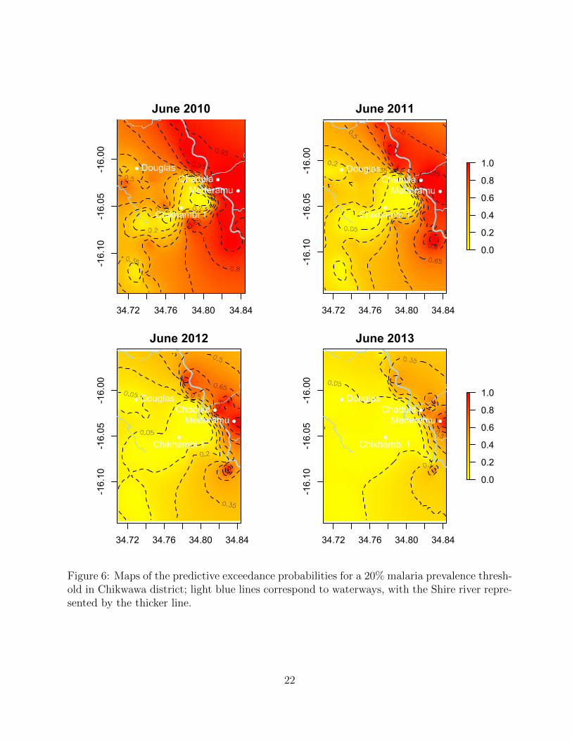
For any specified policy-relevant prevalence threshold p, a quantity of interest is the predictive

probability that the estimated prevalence p(x, t) exceeds p. In Figure 6, we map the exceedance

probabilities in June of each year for p = 0.2. Two areas of high and low prevalence are clearly

identified. The former corresponds approximately to a flooding area where the the presence

of local ponds also favours mosquito breeding.

20

Month

RD

T pr

eval

ence

M J S N J M M J S N J M M J S N J M M

0.00.20.40.60.81.0

Chikhambi 1DouglasChadulaMederamu

2010 2011 2012 2013

Figure 5: Estimated temporal trend of RDT prevalence for four villages in Chikwawa District.Figure 6 shows the location of each of these five villages.

5.1.2 Estimating the impact of scaling-up control interventions

The model (12) that we used to predict malaria prevalence throughout the study-region nec-

essarily excluded any covariate that was only available at the sampled locations. We now

propose a procedure to estimate community-wide prevalence and number of infected children

under a pre-defined control scenario, focusing on the effects of ownership of ITN and presence

of IRS, and adjusting for a measure of each household’s socio-economic status (SES, scored

from 1 to 5). We first fit a model with linear predictor of the same form in (12), but including

these three additional explanatory variables. The resulting parameter estimates are shown in

Table 3 (Model 2). We then use enumeration data to obtain, for each village, the total number

of children under five years and the number of households with at least one child under five

years, and proceed as follows.

(i) Allocate the number of children in each household.

(ii) Impute geographical coordinates, ownership of ITN, presence of IRS and remaining

explanatory variables for all unsampled children under the pre-defined control scenario.

(iii) Generate values for all the model parameters using the asymptotic distribution of the

21

34.72 34.76 34.80 34.84

-16.10

-16.05

-16.00

June 2010

Chikhambi 1

DouglasChadulaMederamu

34.72 34.76 34.80 34.84-16.10

-16.05

-16.00

June 2011

0.0

0.2

0.4

0.6

0.8

1.0

Chikhambi 1

DouglasChadulaMederamu

34.72 34.76 34.80 34.84

-16.10

-16.05

-16.00

June 2012

Chikhambi 1

DouglasChadulaMederamu

34.72 34.76 34.80 34.84

-16.10

-16.05

-16.00

June 2013

0.0

0.2

0.4

0.6

0.8

1.0

Chikhambi 1

DouglasChadulaMederamu

Figure 6: Maps of the predictive exceedance probabilities for a 20% malaria prevalence thresh-old in Chikwawa district; light blue lines correspond to waterways, with the Shire river repre-sented by the thicker line.

22

maximum likelihood estimator, i.e.

θ ∼ N(θ, I−1obs

)where θ is the vector of model parameters and Iobs is the observed Fisher information

as estimated by the negative Hessian of the Monte Carlo likelihood.

(iv) Generate predictive samples for each child’s infection status and compute the mean of

each sample as a point-estimate of the probability of infection for that child.

(v) For each village, estimate of the number of infected children as the sum of the estimated

child-specific probabilities of infection, and average these to estimate the village-level

prevalence.

In Step (ii), we imputed the locations of unsampled children by independent random sampling

from the uniform distribution over each village area Ai, defined as the convex hull of the

sampled households’ locations.

We repeat the above process N times and, for each village, compute summary statistics of the

N samples of estimated numbers of infected children and village-level prevalence. We applied

this procedure under two different scenarios for April 2013, the most recent peak in RDT

prevalence within the period covered by the data, as follows.

S1. Households having IRS and at least one ITN are equally distributed among sampled

and unsampled households.

S2. Every household, whether sampled or unsampled, has IRS and at least one ITN.

In scenario S1, we imputed age, ITN, IRS and SES by random sampling from the empirical

villlage-level distribution of the sampled households. In scenario S2, only SES and age need

23

0 2000 4000

Prevalence reduction0.2% - 1.2%1.2% - 2.2%2.2% - 3.2%3.2% - 4.2%4.2% - 5.2%

OpenCycleMap

0 2000 4000

Cases reduction0 - 23 - 45 - 67 - 89 - 10

OpenCycleMap

Figure 7: Estimated reduction in prevalence (left panel) and number of infected children (rightpanel) for each of the 50 villages in Chikwawa District, assuming a scale-up in the distributionof ITN and IRS to 100% coverage.

to be imputed as ITN and IRS are both present in every household. The differences between

estimated prevalences and between numbers of infected children under S2 and S1 are reported

in Figure 7. The main gains achieved by scenario S2 are in villages situated in the high

prevalence area to the east of the Shire river.

6 Spatially structured zero-inflation

The standard geostatistical model for prevalence data in (2) assumes binomial sampling vari-

ation around the true prevalence, with a latent risk surface that approaches, but does not

exactly reach, zero. However, empirical prevalence data often show an excess of zeros, i.e.

zero-inflation. For diseases that are environmentally driven, one explanation for this is that

some areas are fundamentally unsuitable for disease transmission. Hence, a zero prevalence

estimate in a particular community can be either a chance finding, or a necessary consequence

24

of the community being disease/infection-free. Ways of handling spatially structured zero-

inflation have been proposed in ecology (Agarwal et al., 2002) and in specific epidemiological

applications (Amek et al., 2011; Giardina et al., 2012). These approaches assume that the

zero-inflation can be explained by regressing on a limited set of measured risk factors. In this

extension to the standard geostatistical model (2) for spatially varying prevalence, p(x), the

distribution for the prevalence data Y conditional on S now takes the form of a mixture,

P (Yi = y|S(xi)) =

[1− π(xi)] + π(xi)Bin(0;mi, p(xi)) if y = 0

π(xi)Bin(y;m, p(xi)) if y > 0

(14)

where π(xi) ∈ (0, 1) denotes the probability that xi is suitable for transmission of the disease,

log[π(xi)/{1 − π(xi)}] = d(xi)′γ and Bin(y;m, p) denotes the probability mass function of a

binomial distribution with probability of success p and number of trials m. The modelled

prevalence at location x is p∗(x) = π(x)p(x).

An alternative way of specifying the conditional distribution of Y given S is given by the so

called “hurdle” model (Mullahy, 1986). In this case the mixture distribution for Y assumes

the form

P (Yi = y|S(xi)) =

1− π(xi) if y = 0

π(xi)Bin(y;m, p(xi))

1− Bin(0;m, p(xi))if y > 0

. (15)

In our view, (15) is unsuitable for disease mapping for the two following reasons. Firstly,

the model does not distinguish between observing no cases amongst sampled individuals as

a chance finding or as a necessary consequence of the entire community being disease-free.

Secondly, the model can generate unnatural patches of low prevalence around each sampled

location for which no cases are observed amongst sampled individuals.

A natural extension of the models in (14) and (15) that allows zero-inflation to depend on both

measured and unmeasured covariates can obtained as follows. Define an additional stationary

25

Gaussian process T (x) such that

log[π(xi)/{1− π(xi)}] = d(xi)′γ + T (xi). (16)

Further decompose the spatial processes S(x) and T (x) as

S(x) = U1(x) + V (x),

T (x) = U2(x) + V (x)

where U1(x), U2(x) and V (x) are independent Gaussian proccesses. In this formulation, V (x)

accounts for unmeasured factors that jointly affect the risk of the disease at a location x that

is suitable for transmission of the disease and the risk that x is itself suitable for transmission.

However, identification of all of the resulting parameters requires a large amount of data.

A pragmatic response is to assume that V (x) = 0 for all x, i.e. that S(x) and T (x) are

independent processes.

6.1 Application: river-blindness prevalence mapping

We now show an application to river-blindness prevalence data, previously analysed in Zoure

et al. (2014). Here, we restrict our analysis to three of the twenty APOC countries, namely

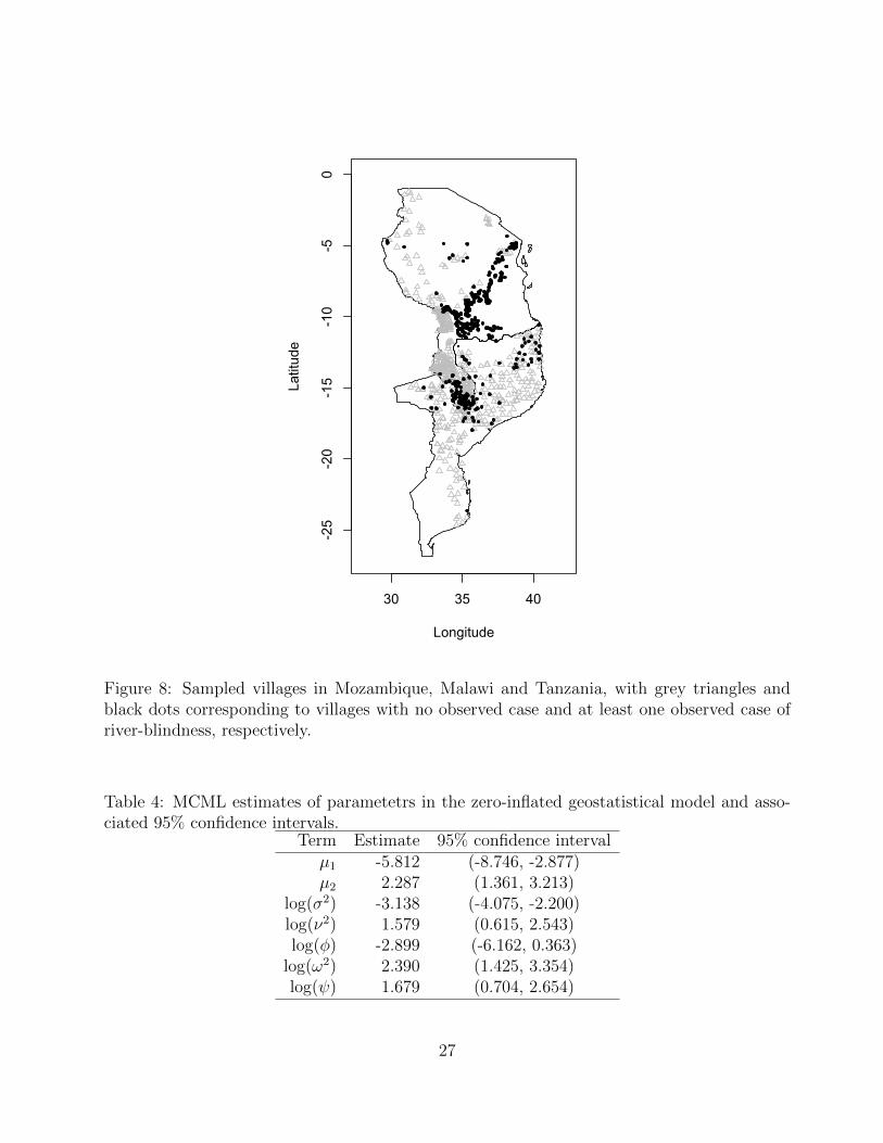
Mozambique, Malawi and Tanzania. Figure 8 shows the locations of the sampled villages in

the three countries. Grey triangles identify the 513 villages with no cases of river-blindness

amongst sampled individuals, black dots the 397 villages with at least one case.

We fit the model with conditional distribution for Y given by (14), and logistic link functions

(2) and (16) for p(x) and π(x), respectively. We also assume that S(x) and T (x) are indepen-

dent processes with covariance functions σ2 exp(−u/φ) and σ2ω2 exp(−u/ψ), respectively; we

denote the variance of the nugget effect Z by σ2ν2. We do include covariates, but simply fit

constant means µ1 and µ2 on the logit-scale of p(x) and π(x), respectively.

26

30 35 40

-25

-20

-15

-10

-50

Longitude

Latitude

Figure 8: Sampled villages in Mozambique, Malawi and Tanzania, with grey triangles andblack dots corresponding to villages with no observed case and at least one observed case ofriver-blindness, respectively.

Table 4: MCML estimates of parametetrs in the zero-inflated geostatistical model and asso-ciated 95% confidence intervals.

Term Estimate 95% confidence intervalµ1 -5.812 (-8.746, -2.877)µ2 2.287 (1.361, 3.213)

log(σ2) -3.138 (-4.075, -2.200)log(ν2) 1.579 (0.615, 2.543)log(φ) -2.899 (-6.162, 0.363)

log(ω2) 2.390 (1.425, 3.354)log(ψ) 1.679 (0.704, 2.654)

27

30 32 34 36 38 40

-25

-20

-15

-10

-5

(a)

-0.2

-0.1

0.0

0.1

0.2

30 32 34 36 38 40

-25

-20

-15

-10

-5

(b)

0.0

0.2

0.4

0.6

0.8

1.0

Figure 9: (a) Difference between predicted prevalences using the standard and zero-inflatedgeostatistical models. (b) Predicted surface π(x).

28

Table 4 shows the MCML estimates of the model parameters. The estimated scale of the

spatial correlation of T (x) is much larger than that of S(x). Also, the estimate of the noise-

to-signal ratio ν2 is substantial.

Figure 9(a) shows the difference between estimates of prevalence ps(x) and pz(x) based on the

standard and zero-inflated, geostatistical models, respectively; these range between plus and

minus 0.2. Figure 9(b) shows the estimated surface of π(x), and indicates that the central

and northern parts of Malawi are disease-free, whereas most of the reported zero cases in

Mozambique and Tanzania are more likely to be attributable to binomial sampling error.

7 Discussion

We have discussed four important issues that arise in prevalence mapping of tropical diseases,

namely: combining data from multiple surveys of different quality; spatio-temporal interpola-

tion of disease prevalence; assessment of the impact of control interventions; and accounting

for zero-inflation in empirical prevalences. For each issue we have presented an extension of

the standard geostatistical model and have described an application that we have encountered

through our involvement with public health programmes in Africa.

In all of our applications, we used the exponential correlation function for the process S. As

discussed in Section 2, this corresponds to the special case of a Matern correlation function

with smoothness parameter κ = 1/2. We did not find evidence against this assumption in any

of our applications. Additionally, in our experience, different choices for κ lead to only small

changes in estimated regression coefficients and the predicted prevalence surface. One reason

for this is that prevalence data are inherently imprecise owing to the inescapable element of

binomial sampling variation. In other application areas, where precise measurement data are

available, the choice between continuous non-differentiable (κ ≤ 1) and differentiable (κ > 1)

members of the Matern family may be more important. Our strategy of choosing between a

29

few values of κ, say κ = 0.5, 1.5 or 2.5, is a pragmatic approach acknowledging that κ is both

poorly identified and typically of limited scientific interest.

As outlined in Section 3, MCML is a useful and feasible computational technique that can be

used to fit a very broad class of generalized mixed models. Compared to techniques based on

analytical approximations of the likelihood function, such as the Laplace approximation (LA),

the MCML method is computationally more intensive. However, subject to computationaly

feasibility, it is more accurate and, especially in the case of small binomial denominators, can

provide more reliable inferences (Joe, 2008).

In the applications of Section 4.1 and Section 5.1, we considered extra-binomial variation at

household-level but not at individual-level within households. An extension of the standard

geostatistical model (2) that accounts for within-household random variation is

log{pij/(1− pij)} = α + [c′ijδ + Uij] + [d(xi)′β + S(xi) + Zi],

where i denotes household, j denotes individual within household, cij is a vector of individual-

specific explanatory variables with associated regression parameters δ and the Vij are mutually

independent, zero-mean, Normally distributed random effects. However, when the data con-

sists of empirical prevalences with small denominators, it is generally difficult to disentangle

the effects of Zi and Uij. For this reason we used the more pragmatic approach of setting

Uij = 0 for all i and j.

The results of Section 5.1.2 on the impact of scaling-up the distribution of ITN and IRS

to 100% coverage should be interpreted cautiously. The procedure that we used to obtain

estimates of prevalence and number of infected children under different scenarios does not

deal with the issue of causation. The control scenarios S1 and S2 represent virtual scenarios

under which coverage of ITN and IRS is assumed to follow a pre-defined pattern without

having any impact on other risk factors for malaria. In reality, a scale-up of ITN and IRS

coverage may influence other features of the process, for example the extent to which ITNs

30

are used correctly.

Under model (14) that accounts for zero-inflation, the risk surface can approach, but not reach,

zero. We are are currently working on two further extensions of the standard geostatistical

model. In the first of these, prevalence can reach zero but is constrained to do so smoothly.

The second allows discontinuities in risk between suitable and unsuitable areas of transmission.

Spatial discontinuities may seem artificial but can give a better fit to the data, especially

when the pattern of risk is highly non-linear. Statistical tools for automatic choice between

non-nested models are available from both frequentist and Bayesian perspectives, but our

preference is to reach agreement with a subject-matter expert on what qualitative features of

the model best reflect the behaviour of the underlying process.

Acknowledgements

We thank the following people for providing the data analysed in the paper and helpful

discussions: Dr. Gillian Stresman and Dr. Jennifer Stevenson (community and school-children

data); Dr. Anja Terlouw (rMIS data); Dr. Hans Remme (river blindness data).

Support was provided by the award of a UK Economic and Social Research Council PhD

studentship (ESRC Grant No.: ES/J500094/1) to Emanuele Giorgi and by The Farr Insti-

tute@HeRC. The Farr Institute@HeRC is supported by a 10-funder consortium: Arthritis Re-

search UK, the British Heart Foundation, Cancer Research UK, the Economic and Social Re-

search Council, the Engineering and Physical Sciences Research Council, the Medical Research

Council, the National Institute of Health Research, the National Institute for Social Care and

Health Research (Welsh Assembly Government), the Chief Scientist Office (Scottish Govern-

ment Health Directorates) and the Wellcome Trust (MRC Grant No.: MR/K006665/1).

31

References

Agarwal, D. K., Gelfand, A. E. & Citron-Pousty, S. (2002). Zero-inflated models

with application to spatial count data. Environmental and Ecological Statistics 9, 341–355.

Amek, N., Bayoh, N., Hamel, M., Lindblade, K. A., Gimnig, J., Laserson, K. F.,

Slutsker, L., Smith, T. & Vounatsou, P. (2011). Spatio-temporal modeling of sparse

geostatistical malaria sporozoite rate data using a zero inflated binomial model. Spatial and

Spatio-temporal Epidemiology 2, 283–290.

Besag, J. & Mondal, D. (2005). First-order intrinsic autoregressions and the de Wijs

process. Biometrika 92, 909–920.

Chiles, J.-P. & Delfiner, P. (2012). Geostatistics: Modelling Spatial Uncertainty. Wiley,

New York, 2nd ed.

Claridge, J., Diggle, P. J., McCann, C. M., Mulcahy, G., Flynn, R., McNair,

J., Strain, S., Welsh, M., Baylis, M. & Williams, D. J. L. (2012). Fasciola hep-

atica is associated with the failure to detect bovine tuberculosis in dairy cattle. Nature

Communications 3, 853.

Clements, A., Lwambo, N., Blair, L., Nyandindi, U., Kaatano, G., Kinung’hi,

S., Webster, J., Fenwick, A. & Brooker, S. (2006). Bayesian spatial analysis and

disease mapping: tools to enhance planning and implementation of a schistosomiasis control

programme in tanzania. Tropical Medicine and International Health 11, 490–503.

Cox, D. R. (1955). Some statistical methods connected with series of events. Journal of the

Royal Statistical Society, Series B 17, 129–164.

Cressie, N. (1993). Statistics for spatial data. Wiley, New York.

De Wijs, H. J. (1951). Statistics of ore distribution. Part I. Frequency distributions of assay

values. Journal of the Royal Netherlands Geological and Mining Society 13, 365–375.

32

De Wijs, H. J. (1953). Statistics of ore distribution. Part II. Theory of binomial distributions

applied to sampling and engineering problems. Journal of the Royal Netherlands Geological

and Mining Society 15, 12–24.

Diggle, P., Thomson, M., Christensen, O., Rowlingson, B., Obsomer, V., Gar-

don, J., Wanji, S., Takougang, I., Enyong, P., Kamgno, J., Remme, J., Boussi-

nesq, M. & Molyneux, D. (2007). Spatial modelling and the prediction of loa loa risk:

decision making under uncertainty. Annals of Tropical Medicine and Parasitology 101,

499–509.

Diggle, P. J., Moraga, P., Rowlingson, B. & Taylor, B. M. (2013). Spatial and

spatio-temporal log-Gaussian Cox processes: Extending the geostatistical paradigm. Sta-

tistical Science 28, 542–563.

Diggle, P. J., Moyeed, R., Rowlingson, B. & Thomson, M. (2002). Childhood malaria

in the Gambia: a case-study in model-based geostatistics. Journal of the Royal Statistical

Society, Series C 51, 493–506.

Diggle, P. J., Tawn, J. A. & Moyeed, R. A. (1998). Model-based geostatistics (with

discussion). Applied Statistics 47, 299–350.

Gemperli, A., Vounatsou, P., Kleinschmidt, I., Bagayoko, M., Lengeler, C. &

Smith, T. (2004). Spatial patterns of infant mortality in Mali: The effect of malaria

endemicity. American Journal of Epidemiology 159, 64–72.

Gething, P. W., Elyazar, I. R. F., Moyes, C. L., Smith, D. L., Battle, K. E.,

Guerra, C. A., Patil, A. P., Tatem, A. J., Howes, R. E., Myers, M. F., George,

D. B., Horby, P., Wertheim, H. F. L., Price, R. N., Meller, I., Baird, J. K. &

Hay, S. I. (2012). A long neglected world malaria map: Plasmodium vivax endemicity in

2010. PLoS Neglected Tropical Diseases 6, e1814.

33

Giardina, F., Gosoniu, L., Konate, L., Diouf, M. B., Perry, R., Gaye, O., Faye,

O. & Vounatsou, P. (2012). Estimating the burden of malaria in Senegal: Bayesian

zero-inflated binomial geostatistical modeling of the MIS 2008 data. PLoS ONE 7, e32625.

Giorgi, E. & Diggle, P. J. (2014). Prevmap: an R package for prevalence mapping.

Submitted.

Giorgi, E., Sesay, S. S. S., Terlouw, D. J. & Diggle, P. J. (2015). Combining data

from multiple spatially referenced prevalence surveys using generalized linear geostatistical

models. Journal of the Royal Statistical Society, Series A 178, 445–464.

Gneiting, T. & Guttorp, P. (2010). Continuous parameter spatio-temporal processes. In

Handbook of Spatial Statistics, A. E. Gelfand, P. J. Diggle, M. Fuentes & P. Guttorp, eds.

Boca Raton: Chapman and Hall/CRC Press, pp. 427–436.

Gotway, C. A. & Stroup, W. W. (1997). A generalized linear model approach to spa-

tial data analysis and prediction. Journal of Agricultural, Biological, and Environmental

Statistics 2, 157–178.

Hay, S. I., Guerra, C. A., Gething, P. W., Patil, A. P., Tatem, A. J., Noor,

A. M., Kabaria, C. W., Manh, B. H., Elyazar, I. R. F., Brooker, S., Smith,

D. L., Moyeed, R. A. & Snow, R. W. (2009). A world malaria map: Plasmodium

falciparum endemicity in 2007. PLoS Medicine 6, e1000048.

Hedt, B. L. & Pagano, M. (2011). Health indicators: Eliminating bias from convenience

sampling estimator. Statistics in Medicine 30, 560–568.

Higdon, D. (1998). A process-convolution approach to modeling temperatures in the North

Atlantic Ocean. Environmental and Ecological Statistics 5, 173–190.

Higdon, D. (2002). Space and space-time modeling using process convolutions. In Quantita-

34

tive methods for current environmental issues, C. W. Anderson, V. Barnett, P. C. Chatwin

& A. H. El-Shaarawi, eds. Springer-Verlag, New York, pp. 37–56.

Joe, H. (2008). Accuracy of laplace approximation for discrete response mixed models.

Computational Statistics & Data Analysis 52, 5066 – 5074.

Kleinschmidt, I., Pettifor, A., Morris, N., MacPhail, C. & Rees, H. (2007). Ge-

ographic distribution of human immunodeficiency virus in South Africa. The American

journal of tropical medicine and hygiene 77, 1163–1169.

Kleinschmidt, I., Sharp, B. L., Clarke, G. P. Y., Curtis, B. & Fraser, C. (2001).

Use of generalized linear mixed models in the spatial analysis of small-area malaria incidence

rates in Kwazulu Natal, South Africa. American Journal of Epidemiology 153, 1213–1221.

Krige, D. G. (1951). A statistical approach to some basiv mine valuation problems on the

witwatersrand. Journal of the Chemical, Metallurgical and Mining Society of South Africa

52, 119–139.

Liang, K. & Zeger, S. L. (1986). Longitudinal data analysis using generalized linear

models. Biometrika 73, 13–22.

Lindgren, F., Rue, H. & Lindstrm, J. (2011). An explicit link between gaussian fields

and gaussian markov random fields: the stochastic partial differential equation approach.

Journal of the Royal Statistical Society: Series B 73, 423–498.

Matern, B. (1986). Spatial Variation. Springer, Berlin, 2nd ed.

Mullahy, J. (1986). Specification and testing of some modified count data models. Journal

of Econometrics 33, 341–365.

Pullan, R. L., Gething, P. W., Smith, J. L., Mwandawiro, C. S., Sturrock, H.

J. W., Gitonga, C. W., Hay, S. I. & Brooker, S. (2011). Spatial modelling of soil-

35

transmitted helminth infections in Kenya: A disease control planning tool. PLoS Neglected

Tropical Diseases 5, e958.

Raso, G., Matthys, B., N’goran, E. K., Tanner, b., Vounatsou, P. & Utzinger,

J. (2005). Spatial risk prediction and mapping of schistosoma mansoni infections among

schoolchildren living in western Cote d’Ivoire. Parasitology 131, 97–108.

Roca-Feltrer, A., Lalloo, D. J., Phiri, K. & Terlouw, D. J. (2012). Rolling malaria

indicator surveys (rMIS): A potential district-level malaria monitoring and evaluation (M

& E) tool for program managers. American Journal of Tropical Medicine and Hygiene 86,

96–98.

Rue, H., Martino, S. & Chopin, N. (2009). Approximate Bayesian inference for latent

Gaussian models by using integrated nested laplace approximations. Journal of the Royal

Statistical Society, Series B 71, 319–392.

Soares Magalhaes, R. J. & Clements, A. C. A. (2011). Mapping the risk of anaemia in

preschool-age children: The contribution of malnutrition, malaria, and helminth infections

in West Africa. PLoS Medicine 8, e1000438.

Stein, M. (1999). Interpolation of Spatial Data: Some Theory for Kriging. Springer, New

York.

Stevenson, J. C., Stresman, G. H., Gitonga, C. W., Gillig, J., Owaga, C.,

Marube, E., Odongo, W., Okoth, A., China, P., Oriango, R., Brooker, S. J.,

Bousema, T., Drakeley, C. & Cox, J. (2013). Reliability of school surveys in estimat-

ing geographic variation in malaria transmission in the Western Kenyan highlands. PLoS

ONE 8, e77641.

Thomson, M., Obsomer, V., Kamgno, J., Gardon, J., Wanji, S., Takougang, I.,

Enyong, P., Remme, J., Molyneux, D. & Boussinesq, M. (2004). Mapping the

36

distribution of Loa loa in Cameroon in support of the African Programme for Onchocerciasis

Control. Filaria Journal 3, 7. DOI:10.1186/1475-2883-3-7.

WHO (2012). African Programme for Onchocerciasis Control: meeting of national onchocer-

ciasis task forces. Weekly epidemiological record 87, 493–508.

Zhang, H. (2004). Inconsistent estimation and asymptotically equal interpolations in model-

based geostatistics. Journal of the American Statistical Association 99, 250–261.

Zoure, Honorat, G. M., Noma, M., Tekle, Afework, H., Amazigo, U. V., Diggle,

P. J., Giorgi, E. & Remme, J. H. F. (2014). The geographic distribution of onchocer-

ciasis in the 20 participating countries of the african programme for onchocerciasis control:

(2) pre-control endemicity levels and estimated number infected. Parasites & Vectors 7.

37