MMT Elevation Servos

D. Clark

August/September 2008

Introduction

• Telescope Design History• Drive System Hardware• LM628 Servo System• Review of Compliantly-coupled

systems• Using Simulink and xPC

Target • Data Collection and Analysis

Tools with Custom Libraries for i/o Hardware and Simulink

• Control Design Methodology

• Elevation Controller Details:» Command preprocessor» Soft-start» Position/Velocity PID loops» Flexible mode filters» Disturbance decoupling» Gain fades for friction and disturbance decoupling

• Tracking data from archives• Recent windup problem• Proposed system

improvements• Final Thoughts

Telescope Design History

• FEA, and other design studies led to an inverted-Serrier truss design

• Friction drives selected with motor-shaft encoders and provision for on-axis tape encoders

• Mandate for commonality with VATT, LBT projects drove early selection of LM628-based controller

FEA Results – SG&H J. Antebi

Model Mode Frequency (Hz) Mode Shape

Overall Telescope 1 4.92 Azimuth torsion

″ 2 5.09 Side-to-side swaying

″ 3 5.25 Nodding in elevation

″ 4 8.17 Twist of f/5 secondary

OSS on rigid support 1 8.15 Twist of f/5 secondary

″ 2 11.7 Nodding in elevation

″ 3 15.8 Side-to-side swaying

″ 4 19.1 In-plane bending of forward frame

Yoke on rigid tower with OSS as a lumped mass

1 5.06 Azimuth torsion

2 5.66 Side-to-side swaying

3 7.14 Nodding in elevation

4 14.85 Side-to-side motion (higher mode)

Elevation Drive

• 2 friction-drive DC brush motors preloaded against a curved truss

• Heidenhain RON905 motor-shaft encoders

• Heidenhain LIDA105C tape encoders

• Inductosyn absolute encoder on-axis

• Copley Model 262 PWM amplifiers.

LM628 Controller

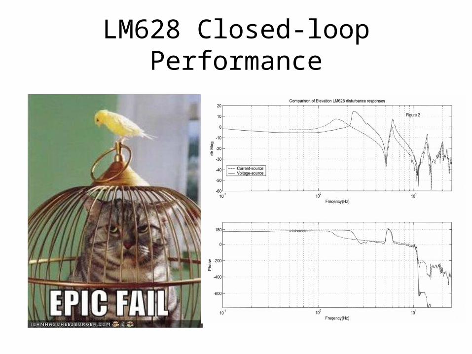
LM628 Closed-loop Performance

Compliantly-coupled Drives

Motor current divided by motor inertia, results in acceleration, which integrates once to velocity. Another integration gives the shaft position. The difference in the position of the motor and load winds up the spring, producing torque, and accelerates the load. The velocity differential likewise slows the motor and speeds up the load.

Compliantly Coupled Motor-Load Transfer Function

The Servo Development Cycle

Collect open-loop input/output data

Construct a mathematical model of the

system

Develop control strategies based on

simulation of the closed-loop system

Measure the closed-loop

system response

Results meet requirements?

Deploy controller

Chirp responses, slewing, tracking

No

Yes

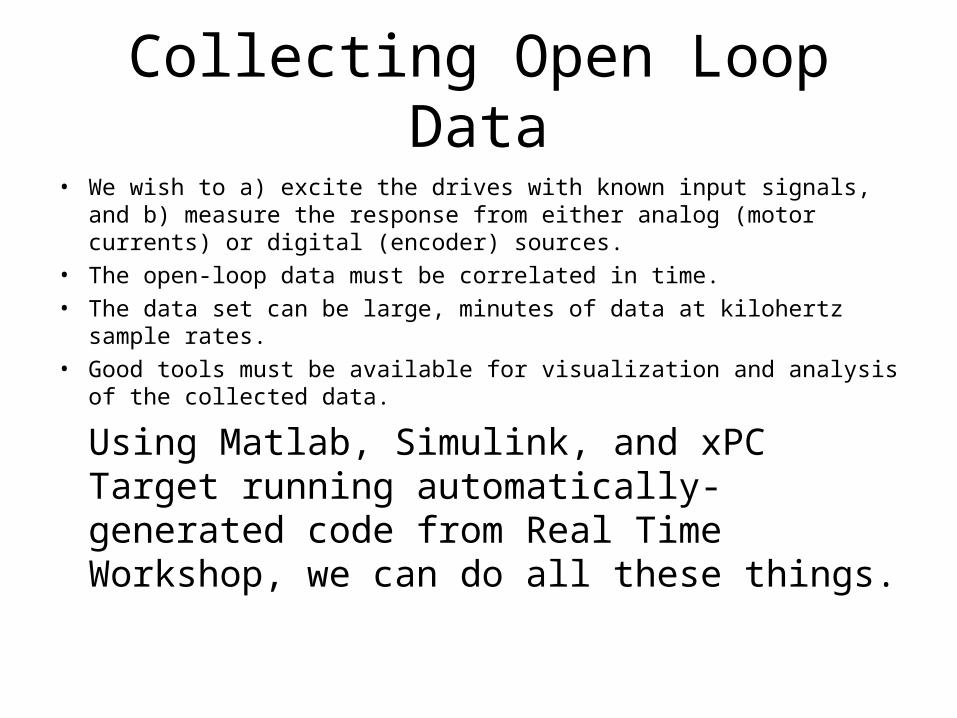
Collecting Open Loop Data

• We wish to a) excite the drives with known input signals, and b) measure the response from either analog (motor currents) or digital (encoder) sources.

• The open-loop data must be correlated in time.• The data set can be large, minutes of data at kilohertz sample rates.• Good tools must be available for visualization and analysis of the

collected data.

Using Matlab, Simulink, and xPC Target running automatically-generated code from Real Time Workshop, we can do all these things.

Introduction to xPC Target

• Think of Simulink as an “engine” to run C code.

• Simulink supports data flow into and out of specific code blocks via an S-function API.

• Simulink can either run the code in simulation mode, or generate an executable version with the help of Real Time Workshop. Soft targets are also available, as rapid-prototyping targets.

• xPC Target is a lightweight realtime kernel for control system prototyping, with tight integration into the Mathworks tool family.

Open Loop Data

Secondary Configurations and Open Loop Response

Modeling and Filter Design

PC Controller Block Diagram

Simplified xPC Controller

P7

P8

tape 2deg 1

-K-

tape 2deg

-K-

Terminator 6

Terminator 5

Terminator 4

Terminator 3

Terminator 2

Terminator 1

Step

Rate Feed Forward

In1 Out1

Position Encoder Handler

Encoder In

Abs In

Position Out

Latched Abs

Filtered Abs

PCI-DAC6703 DA

PCI-DAC6703Measurement

ComputingAnalog Output

1

PCI-60A

PCI-60ASBS

PCI IP Carrier

N-SampleEnable

10

MainLoopLim

Luenberger Observer and Disturbance Decoupling

Tape Position

Command

Feedback

DAC In

DistOut

IP-Quadrature

SBSIP-QuadratureEncoder Input

Goto 5

Reset

From 4

CommandValue

From 22

CommandValue

Elevation Axis Controller - VXWORKS type

Position command DegreesFF

Position command Degrees

Motor Position Degrees

Motor command (DAC volts )

DacOutLim

Create Absolute Angle

In1

In2

Out1

CPP/ no FIR Filter

Cmd

Initial

Out1

Absolute Encoders

IP-Unidig -24Absolute Encoder

Inputs

5-tap Median Filter

Input Output

W tape 50X

The Non-linear Command PreprocessorA nonlinear preprocessor smooths out the position command signal to avoid resonance excitation. Based on W. Gawronski’s work on the Deep Space Network antennas.

In the xPC Target version, this command can be a test signal or position demand over a network connection to a Java GUI. The command can also be set via the GUI to be a tracking command at an arbitrary velocity.

In the VxWorks version, the command is passed via an s-function that hooks to the legacy C code that runs the astronomy and operator GUIs.

In either case this is where all acceleration and velocity limits are applied. This avoids artificially limiting the control bandwidth by having them in the controller’s signal path.

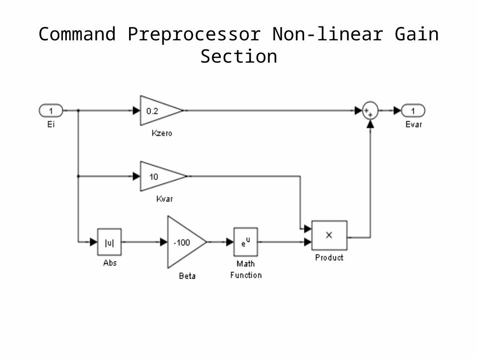
Command Preprocessor Non-linear Gain Section

Absolute Encoder Angle Processing and Position Encoder Handler

Out 1

1

To Deg Conversion

f(u)

S-Function Builder EncoderSynchronizer

encoder _sync

u0

y0

Data Type Conversion 2

Convert

In 2

2

In 1

1

Filtered Abs

3

Latched Abs

2

Position Out

1

SwitchSampleand Hold

In S/H

N-SampleEnable

6

Abs In

2

Encoder In

1

AbsEnc

InitialAbsEnc

AbsPlusTape

The raw coarse and fine encoder data (16 bits each) are meshed together and the resultant 25-bit angle is adjusted to form an absolute angle in degrees.

The absolute encoder position is passed to a transparent latch, where the tape encoder output, which starts at zero and is scaled to degrees is added. The position loop feedback is then absolute tape encoder position, in degrees.

Position and Velocity PID Loops

Motor command (DAC volts )

1

rateff gain

Krff

Velocity Controller

Velocity CMD (deg/s)

Velocity Estimate (deg)

TorqeCommand

SlowStart 1

In1 Out1

SlowStart

In1 Output

Position Controller

Position CMD (deg)

Position (deg)

Velocity CMD (rad)

N-SampleEnable

10

Rst

From

Reset

Flexible ModeCompensation

Unfiltered CMD Filtered CMD

EnabledSubsystem

In1 Out1

Motor PositionDegrees

3

Position command Degrees

2

Position command DegreesFF

1

The position command is differentiated and fed forward as a rate feedforward signal, while the feedback position goes to the position PID loop. Differentiation of the feedback provides the velocity estimate to the velocity loop, and the torque demand is filtered by the filter chain in the Flexible Mode Compensation subsystem. In addition, a reset signal and 10s soft-start blocks provide safe startup when the controller starts running.

PID Loops

Velocity Error

TorqeCommand

1

Velocity gain

Kv_damp

Velocity ControllerProportional gain

Kvp

Velocity ControllerIntegral gain 1

Kvd

Velocity ControllerIntegral gain

Kvi

LTI System

lead _z

Discrete-TimeIntegrator 1

K Ts

z-1

Velocity Estimate (deg )

2

Velocity CMD (deg /s)

1

Velocity CMD (rad )

1

derivative gain

Kd

Proportional gain

Kp

Product

Gain -scheduled Ki

Error_sig Ki_Var

From 23

Feedback

From 22

CommandValue

Discrete-TimeIntegrator 1

K Ts

z-1

DiscreteDifferentiator

numdd

dendd

Position (deg )

2

Position CMD (deg )

1

Both the position loop and velocity loop are straightforward PID, with gain scheduling on the position integral for friction compensation.

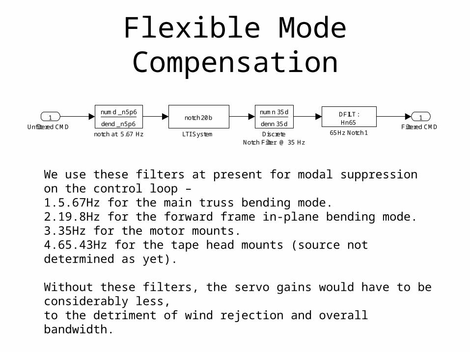
Flexible Mode Compensation

Filtered CMD

1

notch at 5.67 Hz

numd _n5p6

dend _n5p6

LTI System

notch 20 b

DiscreteNotch Filter @ 35 Hz

numn 35 d

denn 35 d65 Hz Notch 1

DFILT :Hn65

Unfiltered CMD

1

We use these filters at present for modal suppression on the control loop –1.5.67Hz for the main truss bending mode.2.19.8Hz for the forward frame in-plane bending mode.3.35Hz for the motor mounts.4.65.43Hz for the tape head mounts (source not determined as yet).

Without these filters, the servo gains would have to be considerably less, to the detriment of wind rejection and overall bandwidth.

Soft-start

Output1

Saturation 2

Product

From

Reset

Discrete-TimeIntegrator

K Ts

z-1Constant

1

1

Soft start is accomplished by integration of a constant, when Reset is not active. The resultant ramp signal is saturated at 1.0 to smoothly bring the signal input from zero to full value on the output of the soft-start subsystem.

Luenberger Observer and Disturbance Decoupling

DistOut

1

Unit Delay 1

z

1

Unit Delay

z

1

Ten Second Ramp

In1 Output

Saturation 2Product 1

Observer Compensator

In1 Out1

Observer

AltElRef

Gain -scheduled Kdd

Error_sig KddVar

DiscreteNotch Filter @ 5.56 Hz

numn 1d

denn 1d DAC In

4

Feedback

3

Command

2

Tape Position

1

Integral Gain and Disturbance Decoupling Gain Scheduling

KddVar

1

ProductMath

Function 1

eu

Gain

60

Constant 1

KddMax

Constant

KddMin

Beta

-1

Abs1

|u|

Error_sig

1

Ki _Var

1

ProductMath

Function 1

eu

Gain

360

Constant 1

Ki * 0.3

Constant

Ki

Beta

-0.02

Abs1

|u|

Error_sig

1

Remarkably similar, the position loop Integral gets scheduled larger when the absolute position error (command minus feedback) is small, and the disturbance decoupling likewise, over different error ranges.

Control Design Validation – Command Signal Path

Control Design Validation – Disturbance Rejection

Comparison of Wind-disturbed Tracking

Wind Shake is a Non-trivial Issue

Servo Progress Report #8 details this set of data, taken with a much earlier version of the xPC Target controller, shows that with the brakes set, the peak-to-peak motion of the drive arcs is still 0.83 arcseconds with winds in the 20s, and gusts to the low 30s. No doubt the motion at the other end of the telescope is proportionally larger, given the compliances and larger moment arm of the OSS.

Tracking Logs• We log tracking data for every object tracked during the night. A web interface makes

the data available for routine inspection of the tracking performance. Here is some data from July 2008. Logs can be found at: http://hacksaw.mmto.arizona.edu/plots/tracking/

• Tracking data can also be triggered on an ad-hoc basis by the operator/engineer.• Data are archived to disk and can be reduced via Matlab scripts written by myself for

detailed analysis – the web interface back-end is based on these.• There is certainly room for improvement in the logging facility:

1. Longer logging time (currently 120s for tracking data) at the full 1kHz servo rate.

2. Ensuring that the mini-server that handles uploading the logging data is robust and always running when data is queued.

3. Having good, correlated wind data for and a facility for quantifying wind angles and tracking error via database queries to build knowledge of best-, worst-, and median-case tracking quality. We recently re-located a wind sensor to improve the agreement of the wind sensors in different locations on the summit.

7/31/08 Collision

Windup Issue

Verification of Windup Cure

More Work to Do

Room for improvement exists in the elevation servo hardware and software:

• Optimize the Luenberger Observer/disturbance decoupling loops.

• Implement 1/T counting for smoother velocity measurements.

• Invest in better absolute encoders (Heidenhain 29-bit absolute units).

• Ensure that both tapes are perfectly square to the rotation axis and the head alignments (new West mount) are the best possible.

• Implement IK220 readout cards with online signal-quality adjustment for the tape encoders.

• Investigate stiffening the motor mounts to eliminate the underconstraint and lost motion.

• Azimuth and rotator axes could benefit from standardization and upgrade efforts, as well.

Final Thoughts• Issues in servo deployment have mainly to do with the wide gulf between the test

environment and deployment environment.• Formal testing and checklists, consistently applied, would help in having a uniform

approach to certification and deployment of controllers, and changes to the controller operation.

• A formal performance specification, other than the very vague one of 0.1 arcsecond RMS tracking over a 10-minute period from the early 6.5m Upgrade documentation, has never been produced. The recent MMT Council specification is extremely ambitious, and certain portions of it cannot be achieved with the telescope we have. Case in point: the AO top-end flexible mode specification can easily be disproven by setting the brakes and capturing all the flexible-mode frequency output from the hub. Since the top end is unencoded, even feedforward of accelerometers down to the drives can’t cure it because there is no motor bandwidth available at those frequencies.

• Followup and documentation from all tests should be done. It’s important to overlay results with one another, or with simulation results, to confirm the outputs are as expected. Further, the deployment environment should support all the same test modes as are available on the test system (e.g. chirp response closed- and open-loop, tracking and slewing, and simulated wind disturbance).

More Final Thoughts

• System behavior and “what-if” scenarios should be checked via simulation to ensure proper operation of the system. Using simulation as a tool allows testing to proceed without endangering people or equipment, and advantage should be taken of those tools.

• Software for both the controller and “other” parts, should always be tested and verified before release to the telescope. Modularization of the code, and testing via simulation, can help in this process. The Mathworks tool family supports several ways of generating reports, adding requirements to tests, and performing code-coverage testing.