MMAE 416 Prof. M. Vural - Illinois Institute of Technologymypages.iit.edu/~vural/RC Airplane Design.pdfMMAE 416 Prof. M. Vural ... trim the aircraft about its center of gravity

MMAE 416 Prof. M. Vural

1

ESTIMATING R/C MODEL AERODYNAMICS AND PERFORMANCE

Adapted from Dr. Leland M. Nicolai’s Write-up (Technical Fellow, Lockheed Martin Aeronautical Company)

by Dr. Murat Vural

(Illinois Institute of Technology) I OVERVIEW

The purpose of this document is to estimate the aerodynamics and performance of an R/C model.

The student needs to understand that the analysis and performance of the R/C model is

identical to a full scale airplane such as a Cessna 172. The only differences between the R/C model and the full scale airplane are the wing loading, Reynolds Number and the moments of inertia.

The R/C model wing loading is one to two orders of magnitude less than a full scale

airplane (because of the “square-cube law” … look it up). R/C models typically have wing loadings of 1-2 lb/ft2 (16-32 oz/ft2) whereas the full scale airplanes are greater than 10 (Cessna 172 is 12.6 lb/ft2). The impact is lower stall speeds and lower take-off and landing distances.

As a general guideline for model R/C airplanes: if the wing loading is under 10 oz/ft2, they will be suitable for the slow flying, gentle handling that you need in electric R/C airplanes used as basic trainers. From 10 to 20 oz/ft2 will include intermediate trainers, flying a little faster, having more power and being a little more demanding in terms of needing a bit more speed for landing and taking off. Above 25 oz/ft2 you begin to find the warbirds, military scale-type models, many of which fly wonderfully, but at the same time are not forgiving of letting the speed get too low while close to the ground.

The R/C model will typically have Reynolds Numbers less than 500,000 which gives

the wing a predominately laminar boundary layer. Full scale airplanes are greater than one million Reynolds Number and have turbulent boundary layer wings. The impact is that the full scale airplanes have higher maximum lift coefficients due to the turbulent boundary layer delaying flow separation over the wing better than the laminar boundary layer. The R/C models and the full scale airplanes are in a Reynolds Number region where the drag coefficients are about the same.

The R/C model will have much smaller moments of inertia than the full scale airplane.

The impact is that the time-to-double-amplitude t2 from a disturbance will be much shorter for the R/C model since t2 = fn (1/(moment of inertia)½ . The R/C pilot will have his hands full with a neutral or unstable model.


2

II DEFINITIONS LIFT: The aerodynamic force resolved in the direction normal to the free stream due to the integrated effect of the static pressures acting normal to the surfaces. DRAG: The aerodynamic force resolved in the direction parallel to the free stream due to (1) viscous shearing stresses, (2) integrated effect of the static pressures acting normal to the surfaces and (3) the influence of the trailing vortices, i.e., inviscid drag-due-to-lift. INVISCID DRAG-DUE-TO-LIFT: Usually called induced drag. The drag that results from the influence of trailing vortices (shed downstream of a lifting surface of finite aspect ratio) on the wing aerodynamic center. The influence is an impressed downwash at the wing aerodynamic center which induces a downward incline to the local flow. (Note: it is present in the absence of viscosity) VISCOUS DRAG-DUE-TO-LIFT: The drag that results due to the integrated effect of the static pressure acting normal to a surface resolved in the drag direction when an airfoil angle-of-attack is increased to generate lift. (Note: it is present without vortices) SKIN FRICTION DRAG: The drag on a body resulting from viscous shearing stress over its wetted surface. PRESSURE DRAG: Sometimes called form drag. The drag on a body resulting from the integrated effect of the static pressure acting normal to its surface resolved in the drag direction. INTERFERENCE DRAG: The increment in drag from bringing two bodies in proximity to each other. For example, the total drag of a wing-fuselage combination will usually be greater than the sum of the wing drag and fuselage drag independent of one another. PROFILE DRAG: Usually taken to mean the sum of the skin friction drag and the pressure drag for a two-dimensional airfoil. TRIM DRAG: The increment in drag resulting from the aerodynamic forces required to trim the aircraft about its center of gravity. Usually this takes the form of added drag-due-to-lift on the horizontal tail. BASE DRAG: The specific contribution to the pressure drag attributed to a separated boundary layer acting on an aft facing surface. WAVE DRAG: Limited to supersonic flow. This drag is a pressure drag resulting from noncancelling static pressure components on either side of a shock wave acting on the surface of the body from which the wave is emanating.


3

COOLING DRAG: The drag resulting from the momentum lost by the air that passes through the power plant installation (ie; heat exchanger) for purposes of cooling the engine, oil and etc. RAM DRAG: The drag resulting from the momentum lost by the air as it slows down to enter an inlet. AIRFOIL: The 2D wing shape in the X and Z axes. The airfoil gives the wing its basic angle-of-attack at zero lift (OL), maximum lift coefficient (Clmax), moment about the aerodynamic center (that point where Cm = 0), Cl,0 for minimum drag and viscous drag-due-to-lift. Two-dimensional airfoil test data is obtained in a wind tunnel by extending the wing span across the tunnel and preventing the formation of trailing vortices at the tip (essentially an infinite aspect ratio wing with zero induced drag). The 2D aerodynamic coefficients of lift, drag and moment are denoted by lower case letters (i.e.; Cl, Cd and Cm) REYNOLDS NUMBER: The Reynolds number is a major similarity parameter and is the ratio of the inertia forces to the viscous forces. The equation for Reynolds number is ⁄ Where = density (kg/m3) V = flight speed (m/s)

l = characteristic length such as wing/tail MAC (mean aerodynamic chord), fuselage length (m)

= coefficient of viscosity (kg/m/s) III APPROACH

We approximate the wing drag polar by the expression

, , ⋯⋯⋯⋯⋯⋯⋯ 1

The first term , is the parasite drag of wing and it is mainly due to skin-friction

and pressure distribution around the airfoil. This term is also referred to as minimum drag ( ). Student must note that minimum drag of the wing and airfoil is indistinguishably close to each other such that , , for all practical purposes.

The second term is the inviscid drag-due-to-lift (commonly referred to as induced

drag) corrected for non-elliptic lift distribution through span efficiency factor “e”. Span efficiency factor can be determined using inviscid vortex lattice codes such as AVL or XFLR5. The “e” for low speed, low sweep wings is typically 0.9 – 0.95 depending on the lift distribution.

Finally, the third term is viscous drag-due-to-lift (which is present even without tip

vortices), where “k” is the viscous factor = fn (LE radius, t/c, camber) and , is the for minimum wing drag.


4

The “k” term is difficult to estimate and is often omitted. However, for a more

accurate analysis it is usually determined from 2D airfoil test data (or airfoil analysis codes such as XFOIL, XFLR5, Profili, etc.) as described below. Here, the ClarkY airfoil is used as an example to demonstrate the process. The parameters , , k and , are determined from airfoil data as shown in Fig. 1. For 2D airfoil data, where induced drag does not exist, Eqn. (1) can be recast as

, , ⋯⋯⋯⋯⋯⋯⋯ 2 Drag polar for 2D airfoil data is fitted by the quadratic function of Eqn. (2) to find the

fitting parameters , , k and , as schematically shown in Fig. 1b.

Figure 1 ClarkY airfoil data at Re = 250,000 from XFLR5 analysis.

Cl,0

Cd,0

(a)

(b)


5

The student must note that fitting process shown in Fig. 1b must be limited to the

range where ∝ relationship is linear (see Fig. 1a), and the focus must be placed on the part of the drag polar that is most useful for the design purpose, i.e., positive lift side. From the fitting process just described above it is found that the best fit to 2D airfoil drag polar data is obtained for

, 0.0145; 0.0664; , 0.4

and the corresponding fitting curve of Eqn. (2) is shown in Fig, 1b with dashed line.

Transition from 2D airfoil data to 3D wing data is done by substituting the fitting

paramaters (obtained in previous step) in Eqn. (1). Thus, with the proper choice of span efficiency factor “e”, Eqn. (1) can be used to represent the drag polar of 3D wing as shown in Fig. 2. In the current example, span efficiency factor 0.95 is used for the best fit to wing data obtained from XFLR5 analysis. When such wing data is not available a proper value of “e” must be chosen depending on the span-wise lift distribution (which is governed by the aspect ratio and taper ratio of the wing).

Figure 2 ClarkY airfoil and wing data at Re = 250,000 from XFLR5 analysis.

IV AIRFOIL AND WING DATA

The 2D airfoil lift data also needs to be corrected for finite wing effects. These correction will be discussed below using the ClarkY airfoil as an example as shown in Figure 3. The ClarkY airfoil is a 11.71% thick cambered shape with its maximum thickness at 28% chord. (Some of the other airfoils typically used by the SAE Aero Design teams are the Selig 1223, Liebeck LD-X17A, and Wortman FX-74-CL5 1223).


6

The first thing the user needs to check is that the data is for the appropriate Reynolds

Number. If we assume a zero-altitude, standard day conditions and a flight speed of 15 m/s (~35.5 mph), the = 1.23 kg/m3 , = 1.789x10-5 kg/m/s, characteristic length of 0.25 m; the Reynolds Number is about 250,000. Thus the airfoil data of Fig. 3 will be good for a wing having a chord of about 0.25m (10").

Figure 3 ClarkY airfoil and wing data at Re = 250,000 from XFLR5 analysis.

From the airfoil data in Fig. 3 the section 1.4 can be determined for a 2D

∝ 12°. Student must notice (from Fig. 1a) that the airfoil has a nasty inverted stall at ∝ 7° (i.e.; the lower surface is separated). Since we do not plan on operating at negative this is OK.

The section lift data needs to be corrected for 3D, finite wing effects. The low speed

unswept finite wing lift curve slope can be estimated as follows for AR > 3:

∝ ∝

∝

2 √4⋯⋯⋯⋯⋯⋯⋯ 3

where ∝= section lift curve slope (typically 2 per radian for high Re numbers)

and wing aspect ratio = (span)2/wing area = ⁄

Note that ∝

tends to be less than 2 at low Re numbers. Figure 3 shows the

construction of a three dimensional AR = 5.2 wing lift curve using the 2D section (airfoil) lift curve slope. The ∝ is an anchor point for constructing the 3D wing lift characteristics since at ∝ the lift is zero and there is no correction to the 3D lift curve for the trailing vortices. Estimate the 3D wing lift curve slope for the model aspect ratio

.


7

using Eqn. (3) and draw it on the . ∝ as shown in Fig. 3. For large AR (i.e.; AR > 5) low speed, unswept wings, the wing 0.9 1.26. The 3D ∝ is approximated using the 2D stall characteristics and is about 14º.

V ESTIMATING MODEL DRAG Similar to the wing drag, we will approximate the aircraft drag polar by the

expression

, ⋯⋯⋯⋯⋯⋯⋯ 4

This expression is slightly different from Eqn. (1) in the first term. Here the CDo is

made up of the pressure and skin friction drag from the fuselage, wing, tails, landing gear, engine, etc. With the exception of the landing gear and engine, the CDo contributions are primarily skin friction since we take deliberate design actions to minimize separation pressure drag (i.e.; fairings, tapered aft bodies, high fineness ratio bodies, etc).

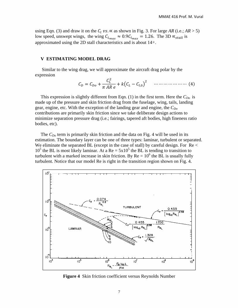
The CDo term is primarily skin friction and the data on Fig. 4 will be used in its

estimation. The boundary layer can be one of three types: laminar, turbulent or separated. We eliminate the separated BL (except in the case of stall) by careful design. For Re < 105 the BL is most likely laminar. At a Re = 5x105 the BL is tending to transition to turbulent with a marked increase in skin friction. By Re = 106 the BL is usually fully turbulent. Notice that our model Re is right in the transition region shown on Fig. 4.

Figure 4 Skin friction coefficient versus Reynolds Number


8

We will demonstrate the methodology by estimating the drag of a notional R/C model

with the following characteristics:

Configuration: Fuselage extending from electric motor at the nose to the tail section. Fuselage length = 50 in, Fuselage width = 5 in Wing AR = 5.2, Wing taper = 0 Wing area = SRef = 504 in2 (total planform area) Wing span = 51.2 in Landing gear: tail dragger (2 main gears and a rear tailwheel) Take-off weight w/o payload = 5 lb Item Planform Wetted Reference Area Area Length (in2) (in2) (in) Fuselage 170 680 50 Wing (exposed) 454 908 9.8 (MAC) Horiz Tail 75 150 5 (MAC)

Vert Tail 0 96 6 (MAC) Landing gear 10 24 na

Engine /mount 5 10 na

The drag coefficients for the model components are estimated as follows for an airspeed of 20 m/s = 44.7 mph (all based on SRef = 504 in2 ). Fuselage Re = 68,500*20*1.27 = 1,740,000, assume BL is turbulent Fuselage CDo = FFF Cf SWet/SRef (5)

Where FF is a form factor representing a pressure drag contribution. Form factors are empirically based and can be replaced with CFD or wind tunnel data. SWet is the wetted area of the component (fuselage) and the Cf is the skin friction coefficient of the component (fuselage) determined from Figure 4 (Cf = 0.0041).

FFF = 1 + 60/(FR)3 + 0.0025 FR (6)

For our model the FR = fuselage fineness ratio = fuselage length/diameter = 50/5 = 10 giving a FFF = 1.085 and a fuselage CDo = 0.0060

Wing Re = 68,500*20*0.249 = 341,000 Wing Cd,o = FFw Cf SWet/SRef (7)


9

Where FFw = [1 + (0.6/(x/c)m)*(t/c) + 100(t/c)4] (8) for a low speed, unswept wing, and (x/c)m is the maximum t/c location of the airfoil (0.28). This, FFw = 1.27 Since a wing Re = 341,000 could be either laminar or turbulent, we will calculate the minimum drag coefficient both ways and compare with the section Cd,o = 0.0145 obtained from XFLR5 (from Figure 1). If the BL is laminar, the wing Cf = 0.00227 and wing CDo = 0.00519. If the BL is turbulent, the wing Cf = 0.00579 and wing CDo = 0.01324. Thus, the wing boundary layer must be turbulent and we, will use wing CDo = 0.0145.

Horizontal Tail Re = 68,500*20*0.127 = 174,000

The Re = 174,000, therefore we’ll assume the BL is laminar. The tail (both horizontal and vertical) CDo equation is the same as for the wing. For NACA 0006 airfoil to be used in tail; t/c = 0.06 and (x/c)m = 0.30. Thus, the FFht = 1.1213, Cf = 0.0032, and horizontal tail CDo = 0.00107.

Vertical Tail

Re = 68,500*20*0.152 = 208,000 The Re = 208,000, therefore assume the BL is laminar. Thus, Cf = 0.0029. For a t/c = 0.06 and (x/c)m = 0.30, FFvt = 1.1213. These leads to vertical tail CDo = 0.00062. Note that CDo for horizontal and vertical tails can also be computed via XFLR5, and would probably give more realistic results.

Landing Gear

From ”Fluid Dynamic Drag” book (by S.F. Hoerner, 1965, page 13.14), experimental data suggest that a single strut and wheel has a CDo = 1.01 based upon the wheel’s frontal area. Thus, for a taildragger (3 inch diameter, 0.5 inch wide main wheels; and 1 inch diameter, 0.25 inch wide tail wheel) total landing gear CDo = (2)(1.01)(1.5)/504 + (1)(1.01)(0.25)/504 = 0.00651 based upon the wing reference area..

Engine

From ”Fluid Dynamic Drag” book (by S.F. Hoerner, 1965, page 13.4, Figure 13), experimental data suggest that the engine CDo = 0.34 based upon frontal area. For a 4 in2

frontal area the engine CDo = (0.34)(4)/504 = 0.0027 based upon the wing reference area..


10

Total CDo

The total CDo is the sum of all the components. Thus the total model CDo = 0.0060+0.0145+0.00107+0.00062+0.0065+0.0027 = 0.0314 based upon a wing reference area of 504 in2 . Note #1: As a sanity check of our CDo we compare it with a Cessna 172 which has a CDo = 0.0260 based upon a wing reference area of 175 ft2 . Note #2: The wing is the largest drag item due to its large wetted area. The second largest drag item is the landing gear which is the case for all full scale airplanes. This drag can be cut in half by putting wheel fairings over the wheels. Is it surprising that airplane designers go to the trouble of designing retractable landing gears?

Total Drag Expression

Recalling from earlier analysis that 0.95; 0.0664; , 0.4 The drag polar expression in Eqn. (4), i.e.,

,

becomes

0.0314 0.0644 0.0664 0.4 ⋯⋯ 9

The untrimmed (neglecting the horizontal tail drag-due-to lift) model drag polar and L/D are shown on Figure 5.

Figure 5 Notional model aircraft total drag polar and L/D.


11

VI ESTIMATING PERFORMANCE Takeoff The takeoff ground roll distance SG is the distance required to accelerate from V = 0 to a speed VTO, rotate to 0.8 CLmax and have L = W. The 0.8 CLmax is an accepted value to allow some margin for gusts, over rotation, maneuver, etc. Assuming a W = 6.5 lb (5.5 lb model and 1.0 lb payload), altitude = sea level (standard day) and a CLmax = 1.25 (from Figure 3) gives the following VTO

VTO = [2 W/(S 0.8 CLmax)]½ = 12.02 m/s = 27 mph

The takeoff acceleration will vary during the ground roll and is given by the following expression a = (g/W)[(T – D) - FC (W – L)] (10) where g = gravitational constant = 9.81 m/s2 and

FC = coefficient of rolling friction = 0.03 (typical value for a Cessna 172 on an average runway).

Note: A useful ground test is to measure the coefficient of rolling friction for your airplane. The testing is fairly simple using a fish scale to measure the rolling force for different loading conditions. The value for FC can increase dramatically if the landing gear is damaged, the wheels do not track straight or the take-off is in tall grass. The landing gear needs to be sturdy with large diameter wheels. A useful expression for the ground roll distance SG is given by the equation SG = VTO

2/(2 amean) (11) where amean = acceleration at 0.7 VTO

Using the notional model aircraft with the wing at 0º angle of incidence ( for minimum drag during the ground run) and data from Figures 3 and 5 gives Ground roll CL = 0.22 (from Figure 3) Ground roll CD = 0.037 (from Figure 5) CLTO = 0.8*CLmax = 1.00 @ = 11.5 (from Figure 3) The predicted thrust is assumed to be governed by the following expression derived from blade element theory:


12

∗ 12

∗ 21 1

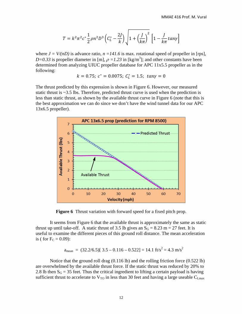
where J = V/(nD) is advance ratio, n =141.6 is max. rotational speed of propeller in [rps], D=0.33 is propeller diameter in [m], =1.23 in [kg/m3]; and other constants have been determined from analyzing UIUC propeller database for APC 11x5.5 propeller as in the following:

0.75; ∗ 0.0075; ∗ 1.5; 0 The thrust predicted by this expression is shown in Figure 6. However, our measured static thrust is ~3.5 lbs. Therefore, predicted thrust curve is used when the prediction is less than static thrust, as shown by the available thrust curve in Figure 6 (note that this is the best approximation we can do since we don’t have the wind tunnel data for our APC 13x6.5 propeller).

Figure 6 Thrust variation with forward speed for a fixed pitch prop. It seems from Figure 6 that the available thrust is approximately the same as static thrust up until take-off. A static thrust of 3.5 lb gives an SG = 8.23 m = 27 feet. It is useful to examine the different pieces of this ground roll distance. The mean acceleration is ( for FC = 0.09):

amean = (32.2/6.5)[ 3.5 – 0.116 – 0.522] = 14.1 ft/s2 = 4.3 m/s2

Notice that the ground roll drag (0.116 lb) and the rolling friction force (0.522 lb) are overwhelmed by the available thrust force. If the static thrust was reduced by 20% to 2.8 lb then SG = 35 feet. Thus the critical ingredient to lifting a certain payload is having sufficient thrust to accelerate to VTO in less than 30 feet and having a large useable CLmax


13

so that VTO is small. Having a headwind will reduce VTO which has a significant effect on SG due to the square of the VTO in the SG equation. After the ground roll, the aircraft rotates to 0.8 CLmax = 1.00 and lifts off. Note that this rotation will take a certain distance (typical rotation time is 1/3 second) and is part of the 30 feet takeoff distance limit. After liftoff the model accelerates and climbs to a safe altitude where the wing is reduced to ~ 4.5 (CL = 0.55 for max L/D) and the power reduced for a steady state L = W, T = D cruise. Maximum Level Flight Speed

The maximum level flight speed occurs when T = D at L = W as shown on Figure 7. For the notional model at L = W = 6.5 lb at sea level the maximum speed is 55 mph (or 24.5 m/s) where T = D ~ 0.87 lb. The drag (required thrust) curve is computed as follows: we first find the CL for L=W as a function of airspeed, then compute CD from drag polar (i.e., from Eqn. 9), and finally calculate the drag for corresponding airspeed.

Figure 7 Thrust available vs. thrust required (drag), and the determination of maximum level flight speed (Vmax).

Documents

MMAE 416 Prof. M. Vural - Illinois Institute of Technologymypages.iit.edu/~vural/RC Airplane Design.pdfMMAE 416 Prof. M. Vural ... trim the aircraft about its center of gravity