Embed Size (px)
Citation preview
Machine Learning Srihari
2
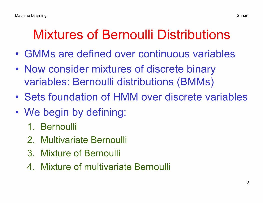
Mixtures of Bernoulli Distributions • GMMs are defined over continuous variables • Now consider mixtures of discrete binary
variables: Bernoulli distributions (BMMs) • Sets foundation of HMM over discrete variables • We begin by defining:
1. Bernoulli 2. Multivariate Bernoulli 3. Mixture of Bernoulli 4. Mixture of multivariate Bernoulli

Machine Learning Srihari
Bernoulli Distribution 1. A coin has a Bernoulli distribution
2. Each pixel of a binary image has a Bernoulli distribution.
– All D pixels together define a multivariate Bernoulli
distribution 3
p(x | µ) = µx(1 − µ)1−x
where x=0,1
Machine Learning Srihari
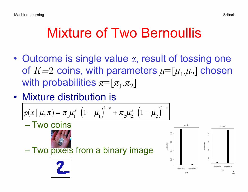
Mixture of Two Bernoullis
• Outcome is single value x, result of tossing one of K=2 coins, with parameters µ=[µ1,µ2] chosen with probabilities π=[π1,π2]
• Mixture distribution is
– Two coins
– Two pixels from a binary image
4
p(x | µ,π) = π
1µ
1x 1 − µ
1( )1−x+ π
2µ
2x 1 − µ
2( )1−x
Machine Learning Srihari
5
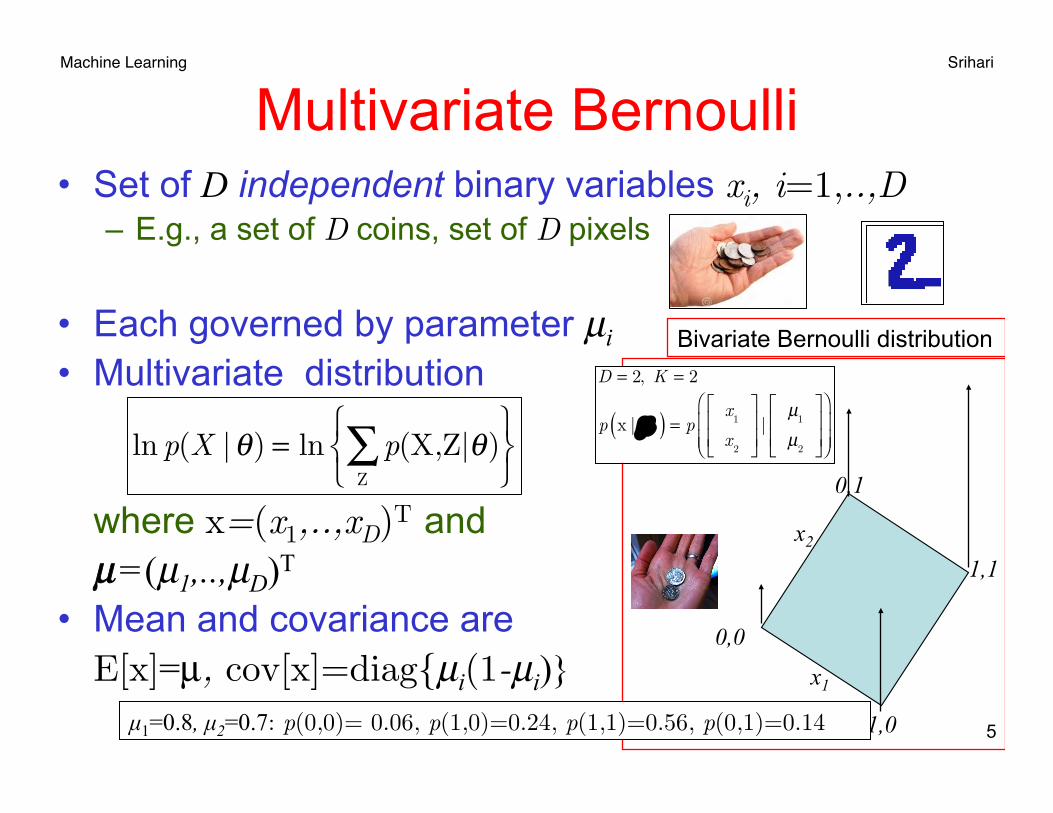
Multivariate Bernoulli • Set of D independent binary variables xi, i=1,..,D
– E.g., a set of D coins, set of D pixels
• Each governed by parameter µi • Multivariate distribution
where x=(x1,..,xD)T and µ =(µ1,..,µD)T
• Mean and covariance are E[x]=µ, cov[x]=diag{µi(1-µi)}
ln p(X |θ) = ln p(X,Z|θ)
Z∑⎧⎨
⎩
⎫⎬⎭
x1
x2
0,0
1,0
1,1
0,1
Bivariate Bernoulli distribution
µ1=0.8, µ2=0.7: p(0,0)= 0.06, p(1,0)=0.24, p(1,1)=0.56, p(0,1)=0.14
D = 2, K = 2
p x | µ( ) = px
1
x2
⎡
⎣⎢⎢
⎤
⎦⎥⎥|
µ1
µ2
⎡
⎣⎢⎢
⎤
⎦⎥⎥
⎛
⎝⎜⎜
⎞
⎠⎟⎟
Machine Learning Srihari
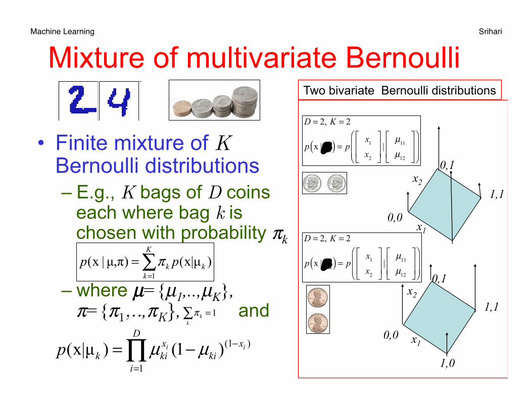
Mixture of multivariate Bernoulli
• Finite mixture of K Bernoulli distributions – E.g., K bags of D coins
each where bag k is chosen with probability πk
– where µ={µ1,..,µK}, π={π1,..,πK}, and
1(x |µ,π) (x|µ )
K
k kk
p pπ=
=∑
(1 )
1
(x|µ ) (1 )i i
Dx x
k ki kii
p µ µ −
=
= −∏ x1
x2
0,0
1,0
1,1
0,1
x1
x2
0,0
1,1
0,1
D = 2, K = 2
p x | µ1( ) = p x1x2
⎡
⎣⎢⎢
⎤
⎦⎥⎥|
µ11µ12
⎡
⎣⎢⎢
⎤
⎦⎥⎥
⎛
⎝⎜⎜
⎞
⎠⎟⎟
Two bivariate Bernoulli distributions
D = 2, K = 2
p x | µ2( ) = p x1x2
⎡
⎣⎢⎢
⎤
⎦⎥⎥|
µ11µ12
⎡
⎣⎢⎢
⎤
⎦⎥⎥
⎛
⎝⎜⎜
⎞
⎠⎟⎟
π kk∑ =1
Machine Learning Srihari
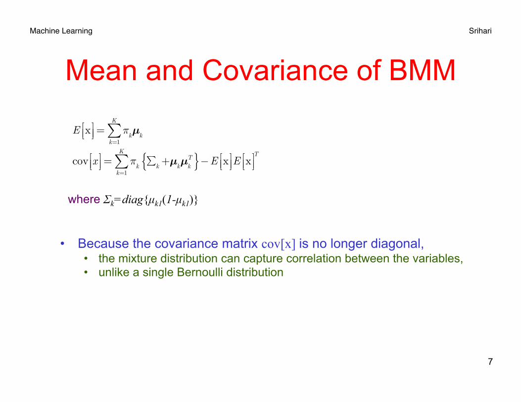
Mean and Covariance of BMM
7
E x⎡⎣⎢⎤⎦⎥ = π
kk=1
K
∑ µk
cov x⎡⎣⎢⎤⎦⎥ = π
kk=1
K
∑ ∑k
+µkµ
kT{ }−E x⎡⎣⎢
⎤⎦⎥E x⎡⎣⎢
⎤⎦⎥T
where Σk=diag{µk1(1-µk1)}
• Because the covariance matrix cov[x] is no longer diagonal, • the mixture distribution can capture correlation between the variables, • unlike a single Bernoulli distribution
Machine Learning Srihari
8
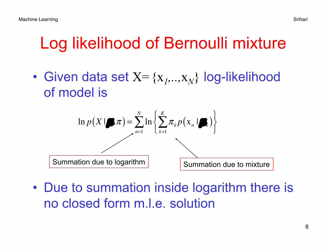
Log likelihood of Bernoulli mixture
• Given data set X={x1,..,xN} log-likelihood of model is
• Due to summation inside logarithm there is no closed form m.l.e. solution
Summation due to mixture Summation due to logarithm
ln p X | µ,π( ) = ln π k p xn | µk( )k=1
K
∑⎧⎨⎩
⎫⎬⎭n=1
N
∑

Machine Learning Srihari
9
To define EM, introduce latent variables
• One of K representation z = (z1,..zK)T
• Conditional distribution of x given the latent variable is
• Prior distribution for the latent variables is same as for GMM
• If we form product of p(x|z,µ) and p(z|µ) and marginalize over z, we recover
1
(x|z,µ) (x|µ ) k
Kz
kk
p p=
=∏
p z | π)( ) = π
k
zk
k=1
K
∏
1(x |µ,π) (x|µ )
K
k kk
p pπ=
=∑
Machine Learning Srihari
10
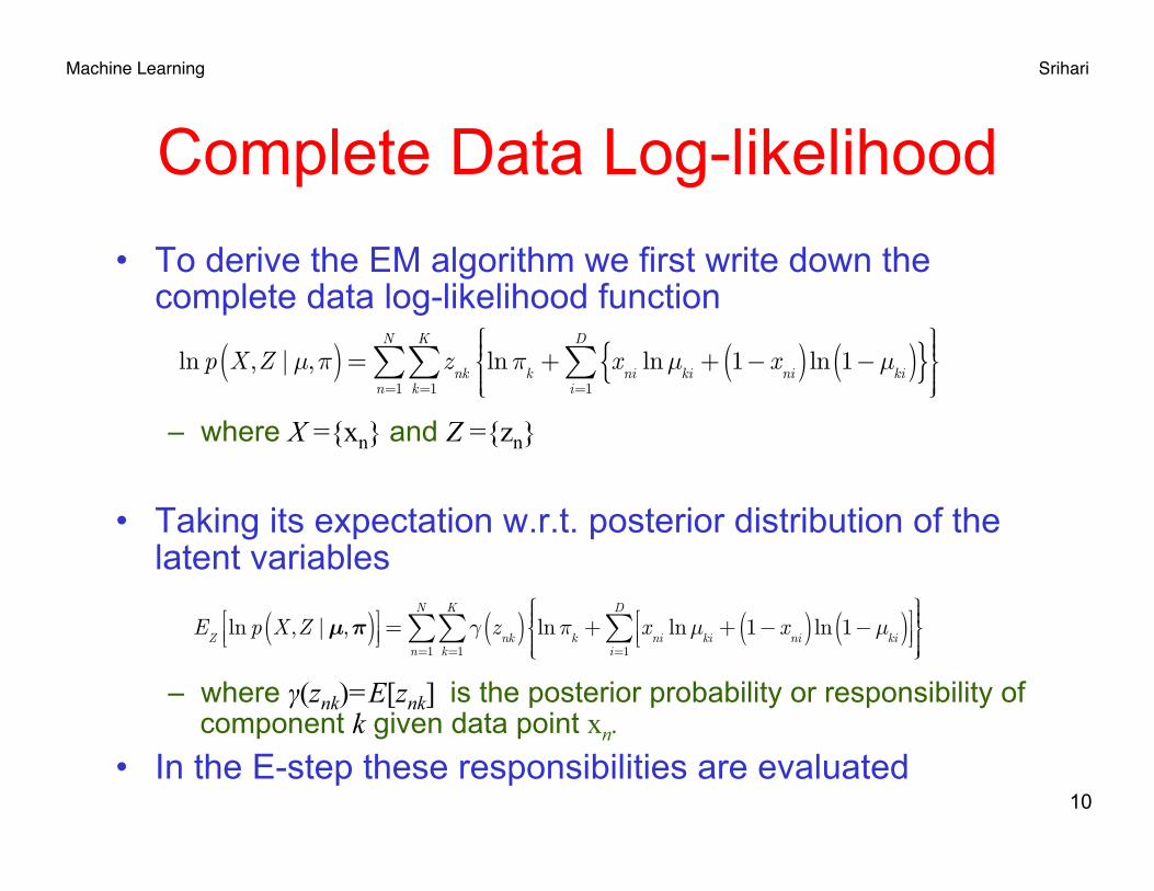
Complete Data Log-likelihood • To derive the EM algorithm we first write down the
complete data log-likelihood function
– where X ={xn} and Z ={zn}
• Taking its expectation w.r.t. posterior distribution of the latent variables
– where γ(znk)=E[znk] is the posterior probability or responsibility of component k given data point xn.
• In the E-step these responsibilities are evaluated
ln p X,Z | µ,π( ) = z
nkk=1
K
∑n=1
N
∑ lnπk
+ xni
lnµki
+ 1−xni( )ln 1−µ
ki( ){ }i=1
D
∑⎧⎨⎪⎪
⎩⎪⎪
⎫⎬⎪⎪
⎭⎪⎪
E
Zln p X,Z | µ,π( )⎡⎣⎢
⎤⎦⎥ = γ z
nk( )k=1
K
∑n=1
N
∑ lnπk
+ xni
lnµki
+ 1−xni( )ln 1−µ
ki( )⎡⎣⎢
⎤⎦⎥
i=1
D
∑⎧⎨⎪⎪
⎩⎪⎪
⎫⎬⎪⎪
⎭⎪⎪

Machine Learning Srihari
E-step: Evaluating Responsibilities • In the E step the responsibilities γ(znk)=E[znk]
are evaluated using Bayes theorem
• If we consider the sum over n in
– Responsibilities enter only through two terms
11
γ znk( ) = E z
nk⎡⎣⎢⎤⎦⎥ =
znkπ
kp x
n| µ
k( )⎡⎣⎢
⎤⎦⎥znk
znk
∑
πjp x
n| µ
j( )⎡⎣⎢
⎤⎦⎥znj
znj
∑
=π
kp x
n| µ
k( )π
jp x
n| µ
j( )j=1
K
∑
E
Zln p X,Z | µ,π( )⎡⎣⎢
⎤⎦⎥ = γ z
nk( )k=1
K
∑n=1
N
∑ lnπk
+ xni
lnµki
+ 1−xni( )ln 1−µ
ki( )⎡⎣⎢
⎤⎦⎥
i=1
D
∑⎧⎨⎪⎪
⎩⎪⎪
⎫⎬⎪⎪
⎭⎪⎪
Nk = γn=1
N
∑ znk( )
xk =1Nk
γn=1
N
∑ znk( )xn
Effective no. of data points associated with component k

Machine Learning Srihari
12
M-step • In the M step we maximize the expected complete data log-
likelihood wrt parameters µk and π• If we set the derivative of
– wrt µk equal to zero and rearrange the terms, we obtain
– Thus mean of component k is equal to weighted mean of data with weighting given by responsibilities of component k for the data points
• For maximization wrt πk, we use a Lagrangian to ensure – Following steps similar to GMM we get the reasonable result
E
Zln p X,Z | µ,π( )⎡⎣⎢
⎤⎦⎥ = γ z
nk( )k=1
K
∑n=1
N
∑ lnπk
+ xni
lnµki
+ 1−xni( )ln 1−µ
ki( )⎡⎣⎢
⎤⎦⎥
i=1
D
∑⎧⎨⎪⎪
⎩⎪⎪
⎫⎬⎪⎪
⎭⎪⎪
µk = xk
π kk∑ =1
π k =Nk
N
Machine Learning Srihari
No singularities in BMMs
• In contrast to GMMs no singularities with BMMs • Can be seen as follows
– Likelihood function is bounded above because 0 ≤ p(xn|µk) ≤ 1
– There exist singularities at which the likelihood function goes to zero
• But these will not be found by EM provided it is not initialized to a pathological starting point
– Because EM always increases value of likelihood function
13

Machine Learning Srihari
14
Illustrate BMM with Handwritten Digits
• Images turned to binary: set values >0.5 to 1, rest to 0
• Fit a data set of N = 600 digits, K=3 • 10 iterations of EM
• Given a set of unlabeled digits 2,3 and 4
• Mixing coefficients initialized with πk=1/K
Parameters µki were set to random values chosen uniformly in range (0.25,0.75) and normalized so that Σjµkj=1

Machine Learning Srihari
15
Result of BMM
Parameters µki for each of three components of mixture model (gray scale since mean for each pixel varies)
Using single multivariate Bernoulli and maximum likelihood amounts to averaging counts in each pixel
EM finds the three clusters corresponding to different digits

Machine Learning Srihari
16
Bayesian EM for Discrete Case • Conjugate prior of the parameters of Bernoulli is
given by the beta distribution • Beta prior is equivalent to introducing additional
effective observations of x • Also introduce priors into the Bernoulli mixture
model • Use EM to maximize posterior probability of
distribution • Can be extended to multinomial discrete
variables – Introduce Dirichlet priors over model parameters if
desired