Mixed thermo-elastohydrodynamic cam-tappet power loss in low speed emission cycle

W.W.F. Chong1, M. Teodorescu2,3 and H. Rahnejat1

1 Wolfson School of Mechanical & Manufacturing Engineering,

Loughborough University, Loughborough, UK 2 School of Engineering, Cranfield University, Cranfield, UK

3 Baskin School of Engineering, University of California at Santa Cruz,

Santa Cruz, USA

Abstract

The key driving forces in engine development are fuel efficiency and emission levels. These aspects are particularly poignant under vehicle idling or low crawling motions in typical city driving. Under these conditions the parasitic frictional losses are exacerbated and the emission levels are especially high. A key engine sub-system is the valve train system. Although it accounts for only 2-3% of the overall engine losses, it is the highest loaded conjunction in the engine, thus limiting the opportunity for lowering the lubricant bulk viscosity. The paper presents detailed tribology of cam-tappet contact, subjected to a mixed thermo-elastohydrodynamic regime of lubrication. In particular, the frictional behaviour of the conjunction is investigated under the stringent North American emission testing city cycle. Such a comprehensive approach has not hitherto been reported in literature. The predictions show good conformance with vehicle frictional assessments in industry. It further demonstrates that under the aforementioned cycle, highest power losses occur which are mainly as the result of lubricant film viscous shear at low sliding speeds and below the lubricant limiting Eyring shear stress.

Keywords: Cam-tappet contact, mixed Thermo-elastohydrodynamics, frictional power loss, low speed city cycle

Nomenclature

a : Contact footprint semi half-width

A : Apparent area of cam-tappet Hertzian contact

b : Cam width (footprint length)

',i ic c : Elemental damping factors

eic : Equivalent damping factor

E : Young’s modulus of elasticity

*E : Effective (reduced) modulus of elasticity of contact

bf : Boundary friction

Tf : Total friction force

vf : Viscous friction

h : Film thickness

0h : Undeformed gap

jψ : Geometrical acceleration

im : Elemental mass

ck : Thermal conductivity of the lubricant

',i ik k : Elemental stiffness

eik : Equivalent stiffness

p : Pressure

cp : Cavitation vaporisation pressure

P : Frictional power loss

R : Instantaneous cam radius of contact

Rb : Base circle radius of the cam

s : Instantaneous cam lift

t : Time

T : Average lubricant temperature in elemental contact strips

0T : Bulk (inlet) oil temperature

avu : Speed of entraining motion

aW : Load share of asperities

hW : Elastohydrodynamic reaction

iW : Total contact force

x : Direction of entraining motion

cx : Cavitation boundary (film rupture location)

iz : Displacement of masses

Z : Lubricant piezo-viscosity index

0α : Lubricant pressure-viscosity coefficient

β : Lubricant bulk modulus

0β : Lubricant temperature-viscosity coefficient

aβ : Average asperity tip radius

δ : Localised contact deflection

γ : Lubricant coefficient of thermal expansion

uΔ : Sliding velocity (2 avu for a stationary tappet)

TΔ : Lubricant temperature rise in elemental contact strips

η : Effective lubricant dynamic viscosity

0η : Lubricant dynamic viscosity at atmospheric pressure and ambient temperature

κ : Average asperity summit radius

sλ : Stribeck’s oil film parameter

θ : Fraction film content

ρ : Lubricant density

cρ : Lubricant density in the cavitated region

0ρ : Lubricant density at atmospheric pressure and ambient temperature

σ : Root mean square surface roughness of counterfaces

τ : Shear stress

0τ : Eyring shear stress

υ : Poisson’s ratio

ω : Cam rotational velocity

Ω : Under-relaxation factor

ψ : Cam angle

ζ : Asperity distribution per unit area

1. Introduction The downsizing philosophy in the development of new internal combustion (IC) engines is based upon high output power-to-weight ratio. The aim is to improve fuel efficiency and reduce hydrocarbon emissions, whilst still addressing the customer desire for maintaining or even improving upon the vehicle power. This trend is likely to continue as IC engines are expected to be the main source of propulsion in the short to medium term (5-10 years) for the road transport sector [1]. In the longer term, further downsized engines would likely form a part of a hybrid power system, for example as range-extenders [2,3]. Whilst this philosophy would have a direct effect on fuel consumption and thus emission levels, the main drawback is that much of the experience related to the existing “package” solutions is not readily transferrable to the new engine architectures. Deviation from the age old experience has already led to a plethora of unwanted problems, arising from a host of conflicting requirements. For example, high power-to-weight ratio often leads to NVH (noise, vibration and harshness) concerns [4,5]. This is an issue which was of little concern beyond simple crank balancing only a couple of decades ago. Higher cylinder pressures as the result of a trend towards diesel fuel or direct injection and turbo-charged gasoline engines have had significant cost implications, for example in terms of piston crown surface redesign and some structural integrity issues. Therefore, as improvements are made to the combustion processes with an ever reducing fuel intake, higher applied loads have resulted in the NVH and friction concerns. One of the historical problems with power generation, in general, has been the failure to achieve a systematic energy balance, or in other words produce an idealised conservative system. Thus, the transient imbalance between the input fuel energy and the useful work done invariably manifests itself in the form of heat and mechanical parasitic losses [4]. The latter is dominated by friction, but also increasingly through NVH. The characteristic responses of friction and NVH are also contradictory in nature. When a suitable design strives to palliate one, the problem with the other is often exacerbated. Consequently, detailed analysis of a systematic integrated multi-disciplinary nature is increasingly sought [6]. The current paper is confined to the analysis of a valve train system. Valve trains are good examples of systems where an integrated solution to inertial and flexible body dynamics (elastodynamics) is sought, together with kinematics of the cam-tappet contact, incorporating its complex tribology [7-11]. The tribology of the contact itself is subject to a transient regime of lubrication affected by shear of a thin film of lubricant as well as interaction of the contiguous surfaces. High generated contact pressures set a limit upon the dynamic performance of the system through contact fatigue spalling limit. Furthermore, friction and generated heat impose another limit on the wear performance of the interface and contribute to engine inefficiency. The cam-follower pair is usually the most loaded conjunction within the engine as well as accounting for as much as 2-3% of all the engine parasitic frictional losses.

Additionally, the contact is often starved and also subject to cavitation. This paper provides an integrated multi-physics multi-scale analysis and extends the work of Teodorescu et al [9,12] to include simplified thermal analysis as well as cavitation and starvation phenomena and thus includes their effects on friction.

2. Mathematical Model

2.1 Kinematics and Dynamics

The general framework of the dynamics’ model is based on the method described by Teodorescu et al [9].

a) Schematic view of the mechanism b) Equivalent model

Figure 1 : Dynamic model for the valve train system

The governing equations of motion are obtained, based on the Newton-Euler method as:

mizi + cei zi − zi−1( )− cei+1 zi+1 − zi( )+ kei zi − zi−1( )− kei+1 zi − zi−1( )+Wi = 0 (1)

where, 1,2i∈ and iW is the cam-tappet contact force. The equivalent spring stiffness terms, eik and damping coefficients, eic are obtained as follows:

( ) ( ) ( ) ( )' ' ' '1 1 1 1/ , / , when in contact

0, 0, no contactei i i i i ei i i i i

ei ei

k k k k k c c c c c

k c− − − −

⎧ = + = +⎪⎨

= =⎪⎩ (2)

where, 3 2 3 2 and e ek k c c= = and 1,2i∈ (figure 1)

Equations of motion (1) are solved by a step-by-step marching integration algorithm to obtain accelerations zi , velocities zi and displacements iz . It is clear that the contact force iW is required prior to the solution of equations of motion. This is obtained as:

i h aW W W= + (3)

where: hW is the elastohydrodynamic contact reaction and aW is the load share carried by the asperities:

cx

hW b pdx−∞

= ∫ (4)

Equation (4) assumes a fully flooded inlet boundary condition:

0 at p x= = −∞ (5)

The exit boundary is set at the lubricant film rupture point (cavitation vaporization boundary):

at c cp p x x= = (6)

The contact between the cam and the tappet is assumed to extend to the edges of the cam width, b.

The load share carried by the asperities is a function of the elastohydrodynamic film thickness, h and the composite roughness of the contiguous contacting surfaces, σ , thus the Stribeck oil film parameter,

shλσ

= . Now assuming a Gaussian distribution for the rough contacting

surfaces of the bounding solids (Greenwood and Tripp [13]):

( )a sσW π ζκσ E AF λκ

= 2 *5 2

8 2 ( )15

(7)

Where, *21

EEυ

=−

is the equivalent plane strain elastic modulus of cam and

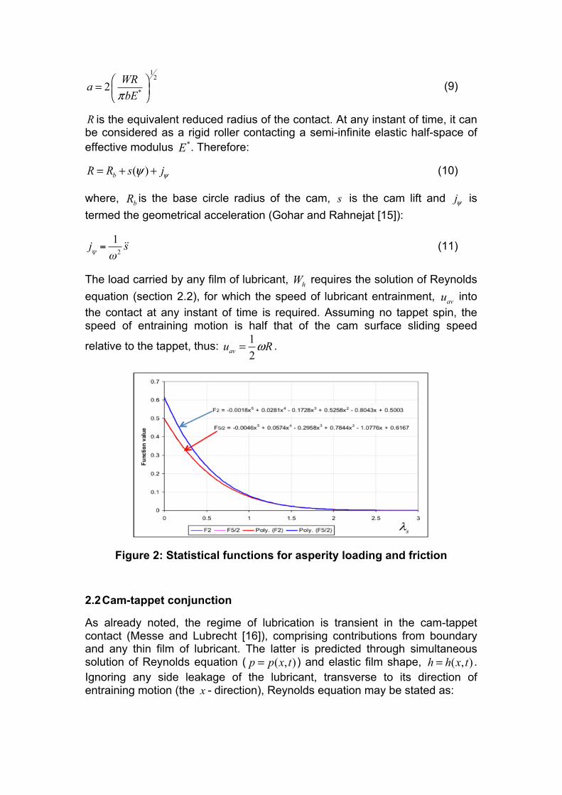
tappet combination, both made of Steel. The statistical function sF λ5 2( ) is fitted by a polynomial function in Teodorescu et al [9,12] and is shown in figure 2. The product ζκσ is the roughness parameter (Tabor [14]) and the

ratio σκ

is a measure of average roughness gradient (Gohar and Rahnejat

[15]). A is the apparent contact area, being a thin rectangular footprint of length b and width 2a , thus:

2A ab= (8)

where, a is calculated using Hertzian contact theory for an elastic line contact as:

12

*2 WRabEπ

⎛ ⎞= ⎜ ⎟⎝ ⎠ (9)

R is the equivalent reduced radius of the contact. At any instant of time, it can be considered as a rigid roller contacting a semi-infinite elastic half-space of effective modulus *E . Therefore:

( )bR R s jψψ= + + (10)

where, bR is the base circle radius of the cam, s is the cam lift and jψ is termed the geometrical acceleration (Gohar and Rahnejat [15]):

jψ =1ω 2s

(11)

The load carried by any film of lubricant, hW requires the solution of Reynolds equation (section 2.2), for which the speed of lubricant entrainment, avu into the contact at any instant of time is required. Assuming no tappet spin, the speed of entraining motion is half that of the cam surface sliding speed

relative to the tappet, thus: 12avu Rω= .

Figure 2: Statistical functions for asperity loading and friction

2.2 Cam-tappet conjunction

As already noted, the regime of lubrication is transient in the cam-tappet contact (Messe and Lubrecht [16]), comprising contributions from boundary and any thin film of lubricant. The latter is predicted through simultaneous solution of Reynolds equation ( ( , )p p x t= ) and elastic film shape, ( , )h h x t= . Ignoring any side leakage of the lubricant, transverse to its direction of entraining motion (the x - direction), Reynolds equation may be stated as:

( ) ( )3

12 avh p u h h

x x x tρ ρ ρη

⎛ ⎞∂ ∂ ∂ ∂⎧ ⎫= +⎨ ⎬⎜ ⎟∂ ∂ ∂ ∂⎩ ⎭⎝ ⎠ (12)

where, the ultimate term on the right hand side is the squeeze film effect, making for a transient analysis of the problem. The speed of entraining

motion, avu and the lubricant squeeze film velocity ht

∂∂

constitute the

instantaneous contact kinematics.

The elastic film shape is: 0 ( )h h s x δ= + + (13)

The instantaneous localized contact deflection is obtained through the solution of elasticity potential integral (Gohar and Rahnejat [15]),

( )1 * 01

1 ( )( )b p x dxx

E x xδ

π=

−∫ , which in discretized form becomes:

2

1

81 ln4

nh

i ij ijj

W RD pδπ=

⎛ ⎞= − ⎜ ⎟

⎝ ⎠∑ (14)

Solution of equations (12)-(14) with lubricant rheological state equations, described below provides the pressure distribution ( , )p x t at any instant of time (section 2.3). This is the approach used by Teodorescu et al [12] and Teodorescu [17].

Reynolds equation does not consider the conservation of mass flow through the cavitation region which is often formed at the trailing edge of the contact. The negative pressures induced by cavitation have a significant effect on the lubricant film thickness and consequently affect the generated viscous friction. In the cam- tappet conjunction, during inlet boundary reversals the formed cavitation region at the trailing edge of the contact becomes its inlet meniscus instantaneously, thus starving the contact of a reservoir of lubricant there. The pre-reversal cavitation leads to the starvation of the contact, reducing the film thickness, thus exacerbating boundary interactions [18]. This phenomenon has not hitherto been taken into account in any previous reported analysis of cam-tappet contact. To account for the effect of cavitation Elrod [19] proposed that the generated pressures are as the result of a fluid film which comprises some liquid lubricant content, θ . This implies that some fractional content of the fluid film may be due to vapour or gaseous content below the lubricant vaporization pressure, cp . Hence:

ln cp g pβ θ= + (15)

where, g is a switching function and β is the bulk modulus of the lubricant, hence:

1 Lubricant film, 10 Cavitation, 0 1

gθθ

⇒ ≥⎧= ⎨ ⇒ < <⎩

(16)

Therefore, when 0g = , a two phase flow below cavitation vaporization

pressure is implied. Now replacing for p from equation (15) into Reynolds equation (12):

( ) ( )3

12cav c c

h g u h hx x x t

ρ θβ ρ θ ρ θη

⎧ ⎫∂ ∂ ∂ ∂⎧ ⎫= +⎨ ⎬ ⎨ ⎬∂ ∂ ∂ ∂⎩ ⎭⎩ ⎭ (17)

It is clear that in the cavitated region, where: 0g = , the Poiseuille flow term on the right-hand side of equation (17) diminishes. The mass flow rate through the cavitation region is, therefore, a balance between the Couette flow due to fluid entrainment and any mutual approach or separation of contiguous surfaces (left-hand side of the equation, Chong et al [18]). 2.3 Lubricant rheological state Lubricant viscosity-pressure variation is predicted using Houpert’s equation [20]:

*

0peαη η= (18)

where, η is the effective viscosity of the lubricant at temperature T and pressure p , and:

0*

0 80

1 138ln 9.67 1 1138 1.98 10

S ZT pp T

α η−⎧ ⎫⎛ ⎞− ⎛ ⎞⎪ ⎪= + + −⎡ ⎤ ⎜ ⎟⎨ ⎬⎜ ⎟⎣ ⎦ ⎜ ⎟− ×⎝ ⎠⎝ ⎠⎪ ⎪⎩ ⎭

(19)

And:

[ ]( )0 00

090 0

138,

5.1 10 ln 9.67 ln 9.67T

Z S−

β −α= =× η + η +

(20)

Also: 0T T T= +Δ , where the rise in the lubricant temperature TΔ is obtained through solution of energy equation (section 2.4). The lubricant density variation with pressure and temperature is obtained as (Dowson and Higginson [21]):

( )9

0 9

0.6 101 11 1.7 10

p Tp

ρ ρ γ−

−

⎛ ⎞×= + − Δ⎜ ⎟+ ×⎝ ⎠ (21)

2.4 Thermal Analysis Viscous shear of a film of lubricant entrained into the conjunction generates friction and results in a rise in the temperature of the lubricant, TΔ . This rise in the lubricant temperature affects its viscosity and density. In particular, the viscosity of the lubricant is reduced, thus resulting in a thinner lubricant film

thickness. In this analysis, any temperature rise as the result of asperity interactions is considered to be localized to the region of their interactions and play a small role in the average temperature rise of the lubricant film. The heat generated by the lubricant flow is as the result of compressive heating of the lubricant as well as through viscous shear. The former is considered to be small compared with the latter in most elastohydrodynamic conjunctions. An order of magnitude analysis in the case of incompressible thin elastohydrodynamic films by Gohar and Rahnejat [15] has shown that compressive heating to be small compared with viscous shear heating. They have also shown that for thin elastohydrodynamic films the heat is carried away from the contact by conduction through the bounding solid surfaces (the cam and the tappet surfaces in this case). Retaining the contribution due to compressive and viscous shear heating, the energy equation is simplified to:

2 2

2av cp u Tu T kx x z

γ η∂ ∂ ∂⎛ ⎞+ = −⎜ ⎟∂ ∂ ∂⎝ ⎠ (22)

Karthikeyan et al [22] provide a simplified analytical solution for equation (22), assuming superposition of compressive and shear heating:

22av

av

au T hp hT ak u hph

ηγ

γ

⎧ ⎫+⎪ ⎪Δ = ⎨ ⎬−⎪ ⎪⎩ ⎭

(23)

where:

0

ηη η= . In this approach a number of other simplifying assumptions

have been made. Firstly, the temperature of the lubricant and the bounding surfaces are assumed to be the same at the inlet to the conjunction and the same as the bulk oil temperature of the engine. In practice, the temperatures of surfaces are higher than the bulk oil temperature at the nib of the contact and thus there is convection from them into the lubricant film there. This rises the temperature of the lubricant above that of the bulk oil temperature. Secondly, within the contact proper, the heat generated is conducted away through the bounding solids. The moving surface (in this case the cam surface) has usually a lower temperature than the lubricant film and a higher temperature than the stationary surface; the tappet. Inclusion of these effects would call for a more complex thermal balance model which should include side leakage of the lubricant (in the y direction), hence an analytical solution would lead to some small inaccuracies. Therefore, the current analysis should be regarded as a simplified thermal model. Equation (23) provides the average temperature in the contact strip of width 2a . To obtain the temperature distribution in the contact, this contact width may be discretised in the same manner as that used for the solution of average flow Reynolds equation (17) and the elasticity potential equation (14). In this case, the inlet temperature in any element of width xΔ is that of the average temperature of a preceding element, i.e. 1i i iT T T−= +Δ . Hence,

equation (23) is solved for each strip of b xΔ at any step of time (crank-angle position) as the cam-tappet contact proceeds in a transient manner. Hence, in equation (23): 2a x= Δ at any instant of time. 2.5 Friction Force

As already noted in the Introduction, prediction of friction is one of the main objectives of any analysis. With thin thermo-elastohydrodynamic films the regime of lubrication is often mixed. Thus, the generated friction is a combination of viscous shear of a thin film of lubricant as well as boundary contribution due to any interactions of asperity pairs on the bounding contiguous surfaces. The contact domain is discretised into a number of elements of area A b xΔ = Δ . The elemental friction can, therefore, be represented in a

differential form as:

T v bdf df df= + (24) where, the viscous friction acts over the lubricated area, which excludes the proportion of the area of an element which represents asperity contact, adA . Thus:

( )v adf dA dAτ= − (25) The shear of the thin film of lubricant formed between the surface asperities is

assumed to follow Newtonian behaviour: ( )( ) ( )avu xx h xητ = , mainly due to

fairly low surface velocities considered in the current analysis (see section 4). However, a thin adsorbed film of molecular dimensions is assumed to exist at the asperity tips (Johnson [23], Greenwood and Tripp [13]). These adsorbed films are subject to non-Newtonian shear (Briscoe and Evans [24] and Chong et al [25]). Thus, boundary friction contribution is obtained as:

0a

b aa

dWdf dAdA

τ ς⎛ ⎞

= +⎜ ⎟⎝ ⎠

(26)

where, 0τ is the Eyring shear stress of the lubricant, ς is the pressure coefficient for boundary shear strength of bounding surfaces and adW is the share of elemental contact load carried by the asperities (Greenwood and Tripp [13]):

( ) ( )2 *52

8 215a a

a

dW dA E fσπ ζβ σ λβ

= (27)

and: ( ) ( )222a adA dA fπ ζβ σ λ= (28)

where, the statistical functions ( )2f λ and ( )52f λ represent the effects of an

assumed Gaussian surface roughness distribution:

( ) ( )2

21 ' '2

snnf s e ds

λ

λ λπ

∞−= −∫ (29)

To expedite the calculation process, these statistical functions are represented by polynomial approximation as proposed by Teodorescu et al [12]. Finally, the total conjunctional friction becomes:

e

i

x

T Tx

f b df dx= ∫ (30)

3 Method of Solution

Vijayaraghavan and Keith [26] proposed the following convenient transformation for the left hand side of equation (17):

( )1g gx xθ θ∂ ∂= −∂ ∂

(31)

Equation (17) can now be written in non-dimensional form as:

( ) ( ) ( )3

1 xc c c

RH g H SX x X b

ρ θ θρ θρη

⎡ ⎤∂ ∂ ∂⎧ ⎫− =Ψ +⎨ ⎬⎢ ⎥∂ ∂ ∂⎩ ⎭⎣ ⎦ (32)

where, 2

hRHa

= , 1

av

hSu t

∂=∂

and 2

03

12 av xu Ra

ηβ

Ψ =

Equation (32) is solved in finite difference form together with non-dimensional forms of equations (13), (14), (18) and (21), using the Effective Influence Newton-Raphson (EIN) low relaxation method with Gauss-Seidel iterations as in Jalali-Vahid et al [27] and Chong et al [18]. For N discrete elements in the direction of entraining motion X:

1

,2

N

i j j ijJ p F

−

=

Δ = −∑ (33)

Where, iF is the residual term and the Jacobian is given as:

( ),i

i jj

FJgθ∂=

∂ (34)

Two convergence criteria are used. The first criterion is based on the fraction film content, θ as:

( )11 2710

k ki i

Nθ θ −

−−

≤∑ (35)

where, the superscript k is an iteration counter. If convergence is not attained, then under-relaxation is employed:

1k k ki i iθ θ θ−= +ΩΔ (36)

where, 1Ω < is an under-relaxation factor. Also:

( ), 1 1 , 1 1

,

k ki i i i i i ik

ii i

F J JJθ θ

θ − − + +− + Δ + ΔΔ = (37)

Once, the convergence criterion (35) is met for all the values of 1,i N= (N being 440 elements in the current analysis), elastohydrodynamic pressures are obtained from equation (15). Then, equations (4) and (7) are employed to obtain the instantaneous total contact load, k

iW from equation (3). This load is compared with that required to satisfy the equation of motion (1), for a given previous iterative value of valve acceleration zi

k−1 , velocity zik−1 and

displacement 1kiz− (i.e. 1k

iW− ). Hence:

1

1 0.01k ki i

ki

W WW

−

−

− < (38)

If the load convergence criterion is not met, the undeformed gap size, 0h is adjusted and the entire iterative process is repeated for any given time step:

10 0 1

kk k i

ki

Wh hW

ξ−

−

⎛ ⎞= ⎜ ⎟

⎝ ⎠ (39)

Where, ξ is damping factor. 4 Results and Discussion

The analysis carried out here concerns the intake valve of a typical cylinder of a 4 cylinder 2 litre diesel engine.. The engine has a bore size of 81 mm and a stroke of 88 mm. There are 4 valves per cylinder; 2 intake and 2 exhaust valves. The analysis is concerned with an intake valve train at the camshaft speed of 630 rpm. This speed represents vehicle crawling in traffic at low speed of 20-40 km/h. The simulated conditions reported here correspond to the North American emission cycle test. Figure 3 shows the variation in the lubricant speed of entraining motion into the contact during the cam event from the valve opening to its closure. The maximum cam lift is at the cam nose-to-tappet contact, designated by the crank-angle of 0o . Note that during the cam event, at the either sides of the cam nose contact there is momentary cessation of lubricant entrainment and a change of sense in the relative velocity of the surfaces. This cessation of lubricant entrainment constitutes thinning of the lubricant film, thus increasing the chance of boundary interactions. Although the phenomenon is short-lived, it constitutes the

instances where greater friction is encountered and also increases the likelihood of wear. The analysis described here concentrates on these regions, in particular during the cam lift event (crank-angle 90 to 0− o o). Here the inlet boundary reversal takes place around the crank-angle of 69.5− o (highlighted by the marked region in figure 3).

Figure 3: Cam lift and speed of entraining motion

Figure 4 shows the contact pressure distribution and film profile for cam transition from valve opening to the cam nose contact, which includes the inlet boundary reversal at the crank angle of 69.5− o. The results are for an inlet oil temperature of 80 Co . Note that the inlet boundary reverses in line with the direction of entrainment velocity shown in figure 3. The secondary pressure peak near the trailing edge of the contact gradually moves across as the direction of entrainment reverses. The contact pressure distribution has a more distinct secondary peak if an isothermal analysis is undertaken, as shown in all the figures. The spatial transition of the secondary pressure peak induces a localized wave front, which creates a moving dimple in the contact surface purely as a kinematic effect, inducing squeeze. This is in line with the observations of Kushwaha and Rahnejat [28], who described this as a squeeze caving phenomenon. The presence of a dimple enhances the lubricant film thickness and reduces the chance of direct boundary interactions. Some have attributed this phenomenon to be the result of thermal effect (Liu et al [29]). The results here show reduced magnitude of secondary pressure peak because of a lower rate of change of viscosity in the vicinity of the contact exit in the thermal contact. This, in turn, reduces the squeeze cave effect as well as decreasing the film thickness.

The simplified thermal model in the current analysis assumes the lubricant temperature and those of the adjacent boundary solids to remain the same. In practice, however, the temperature of the lubricant is higher than the bounding solids, with the moving surface (cam) having a higher temperature than the stationary surface (tappet). The temperature difference is nevertheless quite small and the main effect is from the inlet lubricant temperature, assumed to be that of the bulk oil temperature at the contact

inlet. The average temperature rise above the inlet temperature is shown in figure 5 for various assumed engine bulk oil temperatures. In general, the average temperature rise is quite small and the rise is proportional to the speed of entraining (i.e. viscous shear heating). Therefore, the temperature rise decreases in line with the entrainment velocity variation in figure 3. At the reversal (crank angle of 69.5− o), there is no rise in temperature, because there is momentary cessation of lubricant entrainment. It should be noted that any rise in contact temperature as the result of asperity interactions is ignored in the current analysis. After the inlet reversal, with the commencement of entrainment the lubricant temperature starts to rise again as shown by the the various temperature distributions in figure 6. It is interesting to note that the temperature rise is more notable at lower inlet temperatures, because it is dominated by the ratio h

η . With the same speed of entraining motion and the

applied load, any change in the film thickness is small compared with the variation in η , resulting in a larger change in TΔ . Physically, this finding corresponds to a higher temperature rise in the shear of lubricant film. The lower inlet temperature of 40 Co can represent start-up conditions (or the cold steady state test in the aforementioned emission cycle test), 100 120 C−o o ; the bulk oil temperature in steady engine running conditions (the hot steady state test) and 60 80 C−o o represents the transition period in between (the transient part of the emission test cycle).

(a) -69.5o (b) -68.5o

(c) -67o (d) -66o

(e) -64o

Figure 4: Pressure distribution and corresponding film thickness during inlet boundary reversal

Figure 5: Average lubricant temperature rise in the contact for different inlet temperatures

The minimum film thickness for various inlet temperatures is shown in figure 7. The film thickness reduces with temperature as expected, because of a reduction in the lubricant effective viscosity. Figure 6 shows that the oil film temperature rise in transit through the contact is actually quite low. This is because of the short transit time at any instant of time. Therefore, its viscosity is mainly affected by the inlet temperature. The reduction in the minimum film thickness at any given inlet temperature (figure 7) is because of the reducing speed of entraining motion prior to the inlet reversal at 069.5− cam angle. Thereafter, the speed of entraining motion increases (in the opposite sense) and with an assumed fully flooded inlet the minimum film thickness rises accordingly.

The lubricant is subject to fairly low shear rates because of the low engine speed, thus the sliding velocity in the contact. The viscous shear stress remains below its Eyring value for the lubricant used. The prevailing conditions fall into the Newtonian region in the traction map [15, 30] (figure 8). The ordinate in figure 8 is the speed or rolling viscosity parameter in the form

defined by Grubin [31]: * 0 0

'UURη α= , where for the results shown in the inset to

the figure for the current analysis, 0η η= (the effective viscosity at temperature

0T ), avU u= and 'R R= . The abscissa in the figure is an indication of piezo-viscous behaviour of the lubricant. Note that 1pα = is the demarcation boundary where hydrodynamic inlet pressures are deemed to merge into piezo-viscous lubricant behaviour, and p is the average Hertzian pressure,

1* 21

4WEpRL

π⎛ ⎞= ⎜ ⎟

⎝ ⎠ [15, 30].

(a) -68.5o (b) -67o

(c) -66o (d) -64o

Figure 6: Contact temperature distribution immediately post inlet reversal and at various engine bulk oil temperatures

Contact load (�80o to � 50o)

100

120

140

160

-80 -70 -60 -50

Con

tact

load

(N)

Crank Angle (o)

40oC60oC80oC100oC120oC

Figure 8: Contact load

Minimum film thickness (�80o to � 60o)

0

0.04

0.08

0.12

-80 -75 -70 -65 -60

Min

. Film

Thi

ckne

ss, h

(µm

)

Crank Angle (o)

40oC

60oC

80oC

100oC

120oC

(a) Isothermal analysis

0

0.04

0.08

0.12

-80 -75 -70 -65 -60

Min

. Film

Thi

ckne

ss, h

(µm

)

Crank Angle (o)

40oC

60oC

80oC

100oC

120oC

(b) Thermal analysis

Figure 9: Minimum film thickness

15

Figure 7: Minimum film thickness variation through inlet reversal at different bulk oil temperatures

(a) -80o to -69.5o

Figure 8: Traction behaviour of the lubricant during inlet reversal

It is important to note that lubricant at the tip of opposing asperities on the counterfaces is subject to non-Newtonian shear at the limiting Eyring shear stress (equation (26)). However, this occurs over a very small portion of the contact area and is only significant compared with viscous friction at or near inlet boundary reversals. Figure 9 shows the frictional power loss: TP f u= Δ during half a cam cycle (half the cam lift event). There is slightly greater power loss at higher lubricant temperature because of reduced lubricant viscosity, as well as more boundary interactions on account of a thinner film thickness.

Figure 9: Frictional power loss for half of a cam cycle

The engine power is approximately 1.5 kW under the simulated idling/low crawling speed conditions. For an engine cycle (one camshaft revolution) the maximum frictional power loss from the inlet cam-tappet contact is due to 4 cam event cycles, or approximately 45 W for the cold steady state emission cycle and 50 W for the hot part of the cycle. Therefore, the percentage frictional power loss for the steady state parts of the city cycle is approximately 3%. This is nearly twice the average valve train losses which include a combination of crawling city cycle and vehicle cruising condition as noted by Andersson [32].

5 Conclusion It is shown that the temperature rise in the cam-tappet contact is small compared with the inlet lubricant temperature, which is considered to be the bulk oil temperature in the engine. The reduced effective viscosity of the lubricant due to rising engine temperature promotes a thin film of lubricant few tenths of a micrometer. This promotes mixed elastohydrodynamic regime of lubrication. Simulations of cold and hot steady state low speed driving pertaining to the North American city emission testing cycle show frictional power losses approximately 3% of the engine power. Therefore, in line with expectations low speed city cycle shows poorer valve train efficiency and by implication emissions. An increase in the idling speed would improve the lubricant film thickness but result in higher fuel usage and thus poorer engine efficiency. Thus, any reduction in frictional power should be sought through use of boundary active lubricant species of low shear strength characteristics. The current model does not include the effect of friction modifier species, which is regarded as an area for future research. The conditions investigated here pertain to the low speed city cycle at very low throttle input. With higher partial or wide open throttle conditions higher contact forces result, yielding increased contact pressures and thin films which would lead to non-Newtonian lubricant traction (see the traction map of figure 8). Then, the solution for elastohydrodynamic contact should be based on Ree-Eyring form of Reynolds equation. Therefore, cam-tappet contact is subject to widely

varying conditions and those described in the current paper are concerned with a subset of these, prevalent in low speed city driving.

References

[1]- King, J. The King Review of Low Carbon Cars, The Stationery Office, HM Treasury, UK, ISBN-13: 978-1-84532-335-6

[2] Turner, J., Blake, D., Moore, J. et al “The Lotus Range Extender Engine”, SAE Int. J. Engines, 3(2), 2010, pp. 318-351

[3] Gage, T.B. and Bogdanoff, M.A., “Low-Emission Range Extender for Electric Vehicles”, SAE Trans., Pap. No. 972634, 1997

[4]- Rahnejat, H. Tribology and Dynamics of Engine and Powertrain: Fundamentals, Applications and Future Trends, Woodhead Publishing, 2010, Cambridge, ISBN 10: 1845693612 / 1-84569-361-2

[5]- Menday, M.T., Rahnejat, H. and Ebrahimi, M., “Clonk: An onomatopoeic response in torsional impact of automotive drivelines”, Proc. Instn. Mech. Engrs., Part D: J. Automobile Engng., 213(4), 1999, pp. 349-357 [6]- Boysal, A. and Rahnejat, H. “Torsional vibration analysis of a multi-body single cylinder internal combustion engine”, Appl. Math. Modelling, 21, 1997, pp. 481-493 [7]- Kushwaha, M., Rahnejat, H. and Jin, Z.M. “Valve-train dynamics: a simplified tribo-elasto-multi- body analysis”, Proc. Instn. Mech. Engrs., Part K: J. Multi-body Dyn., 214, 2000, pp. 95-108 [8]- McLaughlin, S. and Haque, I. “Development of a multi-body simulation model of a Winston Cup valvetrain to study valve bounce”, Proc. Instn. Mech. Engrs., Part K: J. Multi-body Dyn., 216, 2002, pp. 237-248 [9]- Teodorescu, M., Kushwaha, M., Rahnejat, H. and Taraza, D. “Elastodynamic transient analysis of a four-cylinder valvetrain system with camshaft flexibility”, Proc. Instn. Mech. Engrs., Part K: J. Multi-body Dyn., 219, 2005, pp. 13-25

[10]- Teodorescu, M., Votsios, V., Rahnejat, H. and Taraza, D. “Jounce and Impact in Cam-Tappet Conjunction Induced by the Elastodynamics of Valve train System”, Meccanica, 41(2), pp. 157-171, 2006

[11]- Guo, J., Zhang, W. and Zuo, D. “Investigation of dynamic characteristics of a valve train system”, Mechanism & Machine Theory, 46(12), 2011, pp. 1950-1969.

[12]- Teodorescu, M., Balakrishnan, S. and Rahnejat, H. “Integrated tribological analysis within a multi- physics approach to system dynamics”, Tribology and Interface Engineering Series (Elsevier), 48, 2005, pp. 725-737

[13]- Greenwood, J.A. and Tripp, J. H. “The contact of two nominally flat rough surfaces” Proc. Instn. Mech. Engrs., Part C: J. Mech. Engng. Sci.,185, 1971, pp.625–633

[14]- Tabor, D. “Surface forces and surface interactions”, J. Colloid & Interface Sci., 58(1), 1977, pp. 2-13 [15]- Gohar, R. and Rahnejat, H. Fundamentals of Tribology, Imperial College Press, London, 2008. [16]- Messe, S. and Lubrecht, A. A. “Transient elastohydrodynamic analysis of an overhead cam/tappet contact”, Proc. Instn. Mech. Engrs., Part J: J. Eng. Trib., 241(5), 2000, pp. 415–425 [17]- Teodorescu, M. “A multi-scale approach to analysis of valve train systems” in Rahnejat, H. (Ed.) Tribology and Dynamics of Engine and Powertrain: Fundamentals, Applications and Future Trends, Woodhead Publishing, 2010, Cambridge, ISBN 10: 1845693612 / 1-84569-361-2 [18]- Chong, W. W. F., Teodorescu, M. and Vaughan, N. D. “Cavitation induced starvation for piston-ring/liner tribological conjunction” Tribology International, 44(4), 2011, pp. 483–497

[19]- Elrod, H. G. “A cavitation algorithm”, Trans. ASME, J. Lubn Tech., 103, 1981, pp. 350–354, 1981

[20]- Houpert, L. “New results of traction force calculations in EHD contacts”, Trans. ASME, J Lubn. Tech., 107, 1985, pp. 241–248

[21]- Dowson, D. and Higginson, G.R. “A numerical solution to elasto-hydrodynamic problem”, J. Mech. Engng. Sci., 1(1), 1959, pp. 6-15

[22]- Karthikeyan, B. K., Teodorescu, M., Rahnejat, H. and Rothberg, S.J. “Thermoelastohydrodynamics of grease-lubricated concentrated point contacts”, Proc. Instn. Mech. Engrs., Part C: J. Mech. Engng. Sci., 224(3), 2010, pp. 683–695

[23]- Johnson, K.L. Contact Mechanics, Cambridge University Press, Cambridge, 1985

[24]- Briscoe B. J. and Evans D. C. B. “The shear properties of langmuir-blodgett layers”, Proc. Roy. Soc. London,. Series A; Math. and Phys. Sci., 380(1779), 1982, pp. 389–407

[25]- Chong, W. W. F., Teodorescu, M. and Rahnejat, H. “Effect of lubricant molecular rheology on formation and shear of ultra-thin surface films”, J. Phys, D: Appl. Phys., 44(16): 165302, 2011

[26]- Vijayaraghavan, D. and Keith Jr., T. G. “Development and evaluation of a cavitation algorithm”, Tribology Transactions, 32(2), 1989, pp. 225–233

[27]- Jalali-Vahid, D., Rahnejat, H., Jin, Z. M. and Dowson, D. “Transient analysis of isothermal elastohydrodynamic circular point contacts”, Proc. Instn. Mech. Engrs., Part C: J. Mech. Engng. Sci., 215, 2001, pp. 1159-1173

[28]- Kushwaha, M. and Rahnejat, H. “Transient concentrated finite line roller-to-race contact under combined entraining, tilting and squeeze film motions”, J. Phys., D: Appl. Phys., 37 (14), 2004, doi:10.1088/0022-3727/37/14/019

[29]- Liu, F., Yang, P., Jin, Z.M. and Dowson, D. “The response of thermal Newtonian and thermal non-Newtonian EHL to the vertical vibration of a roller”, Tribology Series: Transient Processes in Tribology, 43, 2003, pp. 179-187 [30]- Evans, C.R. and Johnson, K. L. “Regimes of traction in elastohydrodynamic lubrication” Proc. Instn. Mech. Engrs., Part C: J. Mech. Engng. Sci., 200 (5), 1986, pp. 313–324 [31]- Grubin, A.N. Contact stresses in toothed gears and worm gears, Book 30 CSRI for technology and Mechanical Engineering, DSRI Trans., 1949, Moscow [32]- Andersson, B.S. “Company's Perspective in Vehicle Tribology- Volvo”, Tribology Series (Elsevier), Vehicle Tribology, 18, 1991, pp. 503-506.