Embed Size (px)
Citation preview
Mixed Control Moment Gyro and MomentumWheel Attitude Control Strategies
C. Eugene Skelton II
Thesis submitted to the Faculty of theVirginia Polytechnic Institute and State University
in partial fulfillment of the requirements for the degree of
Master of Sciencein
Aerospace Engineering
Dr. Christopher Hall, Committee ChairDr. Fred Lutze, Committee Member
Dr. Craig Woolsey, Committee Member
November 21, 2003Blacksburg, Virginia
Keywords: Mixed Control Strategies, Control Moment Gyro, Momentum Wheel,Spacecraft Simulator, Attitude ControlCopyright 2003, C. Eugene Skelton II
Abstract
Mixed Control Moment Gyro and Momentum Wheel Attitude ControlStrategies
C. Eugene Skelton II
Attitude control laws that use control moment gyros (CMGs) and momentum wheels arederived with nonlinear techniques. The control laws command the CMGs to provide rapidangular acceleration and the momentum wheels to reject tracking and initial conditionerrors. Numerical simulations of derived control laws are compared. A trend analysis isperformed to examine the benefits of the derived controllers. We describe the design of aCMG built using commercial off-the-shelf (COTS) equipment. A mixed attitude controlstrategy is implemented on the spacecraft simulator at Virginia Tech.
Acknowledgments
I would like to thank my advisor, Dr. Chris Hall, for his support and patience whileI was coming up the learning curve of spacecraft dynamics and control. Dr. Hall of-fered excellent individual instruction, and should be commended for organizing an idealenvironment for cooperative learning in the lab.
Honeywell Aerospace deserves thanks for funding my research of mixed actuator attitudecontrol. It was their financial support that facilitated the design, construction, andimplementation of a CMG on the spacecraft simulator.
Special thanks goes to the graduate and undergraduate students of the Space SystemsSimulation Laboratory that helped machine, assemble, wire, code, and debug the space-craft simulator, Whorl-I. I would not have simulator results without their assistance.They are (in reverse alphabetical order): Matt VanDyke, Andrew Turner, Bret Street-man, Mike Shoemaker, Jana Schwartz, Marcus Pressl, Scott Lennox, and Cengiz Akinli.
iii
Contents
1 Introduction 1
1.1 Background . . . . . . . . . . . . . . . . . . . . . . . . . . . . . . . . . . 1
1.2 Research Overview . . . . . . . . . . . . . . . . . . . . . . . . . . . . . . 4
1.3 Outline of Thesis . . . . . . . . . . . . . . . . . . . . . . . . . . . . . . . 5
2 Literature Review 6
2.1 Momentum Exchange Devices . . . . . . . . . . . . . . . . . . . . . . . . 6
2.2 Effects of Attitude Representation on Lyapunov Control . . . . . . . . . 8
2.3 Mixed Control Strategies . . . . . . . . . . . . . . . . . . . . . . . . . . . 9
2.4 Spacecraft Simulators . . . . . . . . . . . . . . . . . . . . . . . . . . . . . 10
3 Kinematics and Dynamics 11
3.1 Kinematics . . . . . . . . . . . . . . . . . . . . . . . . . . . . . . . . . . 11
3.1.1 Modified Rodrigues Parameters . . . . . . . . . . . . . . . . . . . 11
3.2 Dynamics . . . . . . . . . . . . . . . . . . . . . . . . . . . . . . . . . . . 12
3.2.1 System Definition . . . . . . . . . . . . . . . . . . . . . . . . . . . 12
3.2.2 Moment of Inertia . . . . . . . . . . . . . . . . . . . . . . . . . . 14
3.2.3 Angular Momentum . . . . . . . . . . . . . . . . . . . . . . . . . 15
3.2.4 Gimbal Angles . . . . . . . . . . . . . . . . . . . . . . . . . . . . 17
3.2.5 Gimbal Momenta . . . . . . . . . . . . . . . . . . . . . . . . . . . 18
3.2.6 Spin Momenta . . . . . . . . . . . . . . . . . . . . . . . . . . . . . 19
3.3 Summary . . . . . . . . . . . . . . . . . . . . . . . . . . . . . . . . . . . 21
iv
4 Controllers 22
4.1 Nonlinear Control Techniques . . . . . . . . . . . . . . . . . . . . . . . . 23
4.1.1 Lyapunov Control Laws . . . . . . . . . . . . . . . . . . . . . . . 23
4.1.2 Feedback Linearization . . . . . . . . . . . . . . . . . . . . . . . . 23
4.2 Reference Motion . . . . . . . . . . . . . . . . . . . . . . . . . . . . . . . 24
4.3 Error States . . . . . . . . . . . . . . . . . . . . . . . . . . . . . . . . . . 24
4.4 Control Moment Gyro Feedback Control Law . . . . . . . . . . . . . . . 25
4.4.1 Singularity Avoidance . . . . . . . . . . . . . . . . . . . . . . . . 26
4.4.2 Singular Direction Avoidance . . . . . . . . . . . . . . . . . . . . 26
4.5 Control Strategy I: Open Loop Control Moment Gyro with Closed LoopMomentum Wheel Control . . . . . . . . . . . . . . . . . . . . . . . . . . 27
4.5.1 Momentum Wheel Lyapunov Control . . . . . . . . . . . . . . . . 28
4.5.2 Momentum Wheel Lyapunov Control with Constant Moment ofInertia Assumption . . . . . . . . . . . . . . . . . . . . . . . . . . 30
4.5.3 Momentum Wheel Lyapunov Control Without Knowledge of theCMGs . . . . . . . . . . . . . . . . . . . . . . . . . . . . . . . . . 30
4.5.4 Momentum Wheel Feedback Linearization . . . . . . . . . . . . . 31
4.5.5 One Open Loop CMG and Momentum Wheel Feedback Control . 32
4.6 Control Strategy II: Control Moment Gyro and Momentum Wheel ClosedLoop Control . . . . . . . . . . . . . . . . . . . . . . . . . . . . . . . . . 33
4.6.1 Parallel Control Moment Gyro and Momentum Wheel Control . . 33
4.6.2 Control Moment Gyro Closed Loop Control with Lyapunov Feed-forward Momentum Wheel Control . . . . . . . . . . . . . . . . . 34
4.7 Summary . . . . . . . . . . . . . . . . . . . . . . . . . . . . . . . . . . . 34
5 Numerical Simulation 36
5.1 System Parameters . . . . . . . . . . . . . . . . . . . . . . . . . . . . . . 37
5.2 Reference Motion . . . . . . . . . . . . . . . . . . . . . . . . . . . . . . . 37
5.3 Control Moment Gyro Gimbal Rate Steering Results . . . . . . . . . . . 39
5.4 Control Strategy I Results . . . . . . . . . . . . . . . . . . . . . . . . . . 39
v
5.4.1 Lyapunov Feedback Control . . . . . . . . . . . . . . . . . . . . . 40
5.4.2 Lyapunov Feedback Control Ignoring ∆I . . . . . . . . . . . . . 40
5.4.3 Lyapunov Feedback Control without CMG Knowledge . . . . . . 41
5.4.4 Momentum Wheel Feedback Linearization . . . . . . . . . . . . . 42
5.4.5 One CMG with Momentum Wheel Feedback Control . . . . . . . 42
5.5 Control Strategy II Results . . . . . . . . . . . . . . . . . . . . . . . . . . 44
5.5.1 Parallel CMG/Momentum Wheel Control . . . . . . . . . . . . . 44
5.5.2 Parallel CMG/Independant Momentum Wheel Control . . . . . . 45
5.5.3 CMG Feedback with Momentum Wheel Feedforward Control . . . 45
5.6 Trend Analysis . . . . . . . . . . . . . . . . . . . . . . . . . . . . . . . . 46
6 Virginia Tech Spacecraft Simulator 53
6.1 Whorl-I . . . . . . . . . . . . . . . . . . . . . . . . . . . . . . . . . . . . 53
6.2 CMG Design . . . . . . . . . . . . . . . . . . . . . . . . . . . . . . . . . 55
6.3 Test Results on Spacecraft Simulator . . . . . . . . . . . . . . . . . . . . 57
7 Conclusions 61
7.1 Summary . . . . . . . . . . . . . . . . . . . . . . . . . . . . . . . . . . . 61
7.2 Recommended Future Work . . . . . . . . . . . . . . . . . . . . . . . . . 62
A Trend Analysis Results without Initial Errors 67
Vita 70
vi
List of Figures
3.1 System with CMGs and Momentum Wheels . . . . . . . . . . . . . . . . 13
3.2 Control Moment Gyro . . . . . . . . . . . . . . . . . . . . . . . . . . . . 14
4.1 Control Organization for CMG Open Loop and Momentum Wheel ClosedLoop Control . . . . . . . . . . . . . . . . . . . . . . . . . . . . . . . . . 28
4.2 Control Organization for CMG and Momentum Wheel Closed Loop Control 33
4.3 Control Organization for CMG and Momentum Wheel Closed Loop Control 34
5.1 Reference Maneuver to be Tracked . . . . . . . . . . . . . . . . . . . . . . 38
5.2 Tracking Reference Body with CMG Feedback . . . . . . . . . . . . . . . 39
5.3 Tracking Reference Body with CMG Feedforward . . . . . . . . . . . . . . 40
5.4 Tracking Reference Body with CMG Feedforward and Momentum WheelLyapunov Feedback Control . . . . . . . . . . . . . . . . . . . . . . . . . 41
5.5 CMG Open Loop with Lyapunov Momentum Wheel Feedback NeglectingdI/dt . . . . . . . . . . . . . . . . . . . . . . . . . . . . . . . . . . . . . . 41
5.6 CMG Open Loop with Independent Lyapunov Momentum Wheel Feedback 42
5.7 CMG Feedforward and Momentum Wheel Feedback Linearization . . . . . 43
5.8 One Open Loop CMG with Lyapunov Momentum Wheel Feedback . . . . 43
5.9 Parallel CMG/Momentum Wheel Control . . . . . . . . . . . . . . . . . . 44
5.10 Parallel CMG/Independent Momentum Wheel Control . . . . . . . . . . 45
5.11 CMG Feedback with Momentum Wheel Feedforward Control . . . . . . . 46
5.12 Control Effort Quantity for CMG Open Loop with Lyapunov MomentumWheel Feedback Control . . . . . . . . . . . . . . . . . . . . . . . . . . . 48
vii
5.13 Control Effort Quantity for CMG Open Loop Control with MomentumWheel Feedback Linearization . . . . . . . . . . . . . . . . . . . . . . . . 48
5.14 Control Effort Quantity for Parallel CMG/Momentum Wheel Control . . 49
5.15 Control Effort Quantity for CMG Feedback Control with Momentum WheelFeedforward Control . . . . . . . . . . . . . . . . . . . . . . . . . . . . . 50
5.16 Maximum Control Torques for CMG Open Loop with Lyapunov Momen-tum Wheel Feedback Control . . . . . . . . . . . . . . . . . . . . . . . . . 50
5.17 Maximum Control Torques for CMG Open Loop Control with MomentumWheel Feedback Linearization . . . . . . . . . . . . . . . . . . . . . . . . 51
5.18 Maximum Control Torques for Parallel CMG/Momentum Wheel Control 51
5.19 Maximum Control Torques for CMG Feedback Control with MomentumWheel Feedforward Control . . . . . . . . . . . . . . . . . . . . . . . . . . 52
6.1 Virginia Tech’s Tabletop Spacecraft Attitude Control System Simulator . 54
6.2 Change in Angular Momentum from Gimballing . . . . . . . . . . . . . . 55
6.3 CMG Implemented on Virginia Tech Spacecraft Simulator . . . . . . . . 56
6.4 Simulator Angular Velocity and Attitude with CMG Actuation Only . . . 58
6.5 Simulator Angular Velocity and Attitude with Momentum Wheel ActuationOnly . . . . . . . . . . . . . . . . . . . . . . . . . . . . . . . . . . . . . . 58
6.6 Simulator Momentum Wheel Control Torques with Momentum Wheel Ac-tuation Only . . . . . . . . . . . . . . . . . . . . . . . . . . . . . . . . . . 59
6.7 Simulator Angular Velocity and Attitude with Mixed CMG and MomentumWheel Actuation . . . . . . . . . . . . . . . . . . . . . . . . . . . . . . . 60
6.8 Simulator Momentum Wheel Control Torques with CMG and MomentumWheel Actuation . . . . . . . . . . . . . . . . . . . . . . . . . . . . . . . 60
A.1 Control Effort Quantity for CMG Open Loop with Lyapunov MomentumWheel Feedback Control without Initial Errors . . . . . . . . . . . . . . . 67
A.2 Control Effort Quantity for CMG Open Loop Control with MomentumWheel Feedback Linearization without Initial Errors . . . . . . . . . . . . 68
A.3 Control Effort Quantity for Parallel CMG/Momentum Wheel Control with-out Initial Errors . . . . . . . . . . . . . . . . . . . . . . . . . . . . . . . 69
A.4 Control Effort Quantity for CMG Feedback Control with Momentum WheelFeedforward Control without Initial Errors . . . . . . . . . . . . . . . . . 69
viii
List of Tables
5.1 Spacecraft Parameters . . . . . . . . . . . . . . . . . . . . . . . . . . . . 37
5.2 Constants and Gains . . . . . . . . . . . . . . . . . . . . . . . . . . . . . 38
5.3 Reference Torque Magnitude and Duration . . . . . . . . . . . . . . . . . 47
6.1 Output Torque with Varying Gimbal Rates . . . . . . . . . . . . . . . . . 56
ix
1
Chapter 1
Introduction
1.1 Background
Spacecraft cover a broad range of missions with differing system requirements. Space-
craft range in size from picosats to space stations. Some spacecraft have autonomous
control, while others have no dynamic control. Spacecraft maneuverability is dependent
on mission requirements.
A common example of a spacecraft with an interesting mission is the Hubble Space Tele-
scope, which must maneuver to and hold an orientation in inertial space. Hubble uses
four reaction wheels and magnetic torquers for attitude control [1]. The time for reori-
entations is on the order of tens of minutes, an acceptable period for Hubble’s mission.
Certainly different missions dictate the acceptable period for a maneuver. A spacecraft
designed to intercept objects coming into the atmosphere might require the ability to
slew one half of a revolution in seconds and then track an object which is moving at
a high velocity. Such large slew, high-rate maneuvers can be achieved with differing
types of actuators, and possibly combinations of actuators. Strategies for maneuvers can
be adapted for attitude maintenance, that are needed because of aerodynamic, gravity
gradient, and solar wind perturbations.
Common actuators for applying torques are thrusters and magnetic torquers. Thrusters
provide torque on the spacecraft by expelling propellant. Magnetic torquers use the
earth’s magnetic field to generate torque on the spacecraft. There are limitations to both
thrusters and magnetic torquers.
Thrusters require propellant, which must be launched with the spacecraft at consider-
1.1 Background 2
able cost. The exhausted propellant can affect sensitive equipment such as optics. The
changing mass of the spacecraft, movement of the center of mass, and changing inertia
tensor, make control laws more complex. Attitude maintenance using thrusters requires
low impulse capability. Low thrust diminishes the rapid slewing ability of a spacecraft.
Advantages of magnetic torquers are that they have no moving components and they do
have replenishment power supply with solar power. However they typically provide small
torque which is not acceptable for rapid slewing. The magnetic field of the earth or any
primary body varies in strength and direction depending on orbital position, which adds
complexity to control derivation and modelling.
Other means of applying torque to a spacecraft involve momentum exchange devices such
as momentum wheels and control moment gyros. Momentum exchange devices work
through the conservation of angular momentum. Conservation of angular momentum
states that the angular momentum of a system without external torques is constant in
the inertial frame. From conservation of angular momentum we know that a body and
flywheel system has an angular momentum equal to the sum of its individual momenta,
and it is constant in the inertial frame for all time provided there are no external torques.
Changing the flywheel’s angular momentum will affect the body’s angular momentum and
vice versa. There are two common devices for angular momentum exchange, momentum
wheels and control moment gyros.
A momentum wheel consists of a flywheel that spins about a fixed axis in the body.
The flywheel is generally axisymmetric and spins about its axis of symmetry. Angular
momentum is exchanged between the flywheel spin axis and the body by applying a torque
with a motor. The acceleration of the body about the spin axis of the momentum wheel is
related to the change in angular momentum of the momentum wheel and the inertia of the
body about the momentum wheel spin axis. Typically there are four momentum wheels
mounted in such a way that there is redundancy for three-axis control. The maximum
acceleration of the body from the momentum wheel is limited by the maximum torque
of the motor.
The control moment gyro (CMG) is a momentum exchange device that can produce
large output torque on the body. A CMG has a flywheel that spins at a constant velocity
relative to the CMG frame. The spin axis of the flywheel can vary about a perpendicular
axis to its spin axis. We call this perpendicular axis the gimbal axis. Complex dynamic
derivations are used to find a relationship between the torque input to gimbal axis and
a desired output torque on the body. The rate of change of angular momentum between
the CMG and the body is dependent on the gimbal velocity. An unwanted result of
varying the spin axis of the flywheel is that there can be orientations where no output
1.1 Background 3
torque can be given in a certain direction; these orientations result in singularities in
the control laws. Typically singularities are avoided by either using a pyramid of four
CMGs or by deriving a controller that is “smart enough” to avoid singular orientations.
Concepts that use other actuators with CMGs or variable-speed CMGs have also been
explored for singularity avoidance.
The concept of mixed actuator attitude control attempts to take advantage of the strong
aspects of certain devices while using other devices to compensate for the weaknesses of
the first set devices. An example is the use of thrusters and momentum wheels [2], where
the thruster provide coarse rapid acceleration and the momentum wheels provide fine
tuning of attitude and angular velocity. Certainly there is the advantage of redundancy
with multiple attitude control actuators; however the price of redundancy is hardware,
launch cost, and control complexity.
The general problem that we address is spacecraft reorientation and high-speed tracking.
More generally the problem is determining the current attitude and angular velocity of
a body, determining a desired attitude and angular velocity, and determining the control
inputs to the devices that will drive the current attitude and angular velocity to the
desired. The means of solving for the inputs can be simple or complex depending on the
devices and initial error between the current and desired states. The control laws that
determine the inputs to the devices have been the subject of many studies.
Another way of thinking about the problem is to determine the path in state space to
get from the current to the desired attitude and angular velocity. The complexity of
path determination is dependent on the devices and the initial error. For any rotation an
Euler axis and Euler angle can be found to be the most direct path between the initial
and desired attitude. The minimum time reorientation is achieved by accelerating at
maximum torque about the Euler axis to half of the Euler angle, and then decelerating
at maximum torque to the desired attitude if the Euler axis is aligned with a principle
axis. The minimum time reorientation uses “bang-bang” control. In real spacecraft
the ability to apply maximum torque about any Euler axis is generally not possible.
Moreover, the off-diagonal terms of the inertia for a spacecraft will cause off-Euler axis
rotations about the Euler axis if the Euler axis does not coincide with a principal axis.
Common means of validating control laws are numerical simulation and implementa-
tion on a physical apparatus that reflects attributes of the real system to be controlled.
Numerical simulations are effective at demonstrating control concepts in an ideal envi-
ronment at minimal cost. For this research numerical simulations of a rigid body with
three CMGs and three momentum wheels are performed without the hardware cost of
each device. Spacecraft simulators are apparatuses for physical implementation that gen-
1.2 Research Overview 4
erally consist of a body with varying rotational and translational freedom. Simulators
can vary from single degree of rotational or translational freedom to full six degree of
freedom systems [3].
The purpose of this research is to explore the use of control moment gyros for rapid coarse
slewing maneuvers and momentum wheels for fine tuning of attitude and angular velocity.
The momentum wheels can adjust for initial condition errors, and tracking errors. The
effectiveness of derived control laws is measured by control effort, accuracy, and time
required for a maneuver. Numerical simulation and implementation on a spacecraft
simulator validate the derived control laws and strategies. ∗
1.2 Research Overview
The goal of this research is to develop control laws that use control moment gyros for
large reorientations or rapid tracking and momentum wheels for error rejection. Ford [4]
developed the equations of motion for a rigid body with gimballed momentum wheels.
Ford’s equations are modified to represent a rigid body with CMGs and momentum
wheels. Equations of motion of a virtual reference body are developed. A body fixed
reference frame in the virtual reference body defines the desired motion for tracking.
Control laws are developed that use angular velocity and attitude feedback for tracking
of a reference trajectory. Modified Rodrigues Parameters (MRPs) are used to describe
the attitude of the body and virtual reference frame. A Lyapunov control law introduced
in Ref. [5] and modified in Ref. [2] is expanded to account for the control moment gyros’
dynamics. A control strategy provides open loop actuation of the CMGs with closed
loop control from the momentum wheels, where the feedback control law may or may
not have knowledge of the CMG’s maneuvering. Various closed loop control laws that
use both CMGs and momentum wheels are developed.
A mathematical model of a rigid body with CMGs and momentum wheels is developed
to evaluate the effectiveness of control laws. The model has full rotational freedom.
Numerical simulation of the control laws are performed.
The control laws derived are tested on the Distributed Spacecraft Attitude Control Sys-
tems Simulator in the Space Systems Simulation Lab at Virginia Tech. A CMG was
designed, fabricated, assembled, tested, and integrated into the simulator with use of
commercial off-the-shelf (COTS) components. Large slew maneuvers are performed on
the simulator to illustrate the control strategy.
∗http://www.aoe.vt.edu/research/groups/sssl/
1.3 Outline of Thesis 5
1.3 Outline of Thesis
A review of the literature is presented in Chapter 2. Specific attention is given to studies
that use CMGs or momentum wheels for attitude control of spacecraft. Work directed
toward reorientations and mixed control strategies is presented. An overview of other
spacecraft simulators is presented.
In Chapter 3 we cover the kinematics and equations of motion for a rigid body with CMGs
and momentum wheels. The attitude representation is Modified Rodrigues Parameters.
The equations of motion are expressed in vector form. The control inputs are momentum
wheel spin axis torques and CMG gimbal axis torques.
Spacecraft reorientations and tracking are addressed in Chapter 4. Error functions for
attitude and angular velocity are defined. Lyapunov control laws are derived for reference
body tracking. A feedback linearization control law is developed for use with the momen-
tum wheels as error rejection. Other strategies that use CMGs and momentum wheels
together in feedback are presented, along with a CMG feedback and momentum wheel
feedforward control law. Several variations of the developed control laws are presented.
For each derived controller numerical simulation results are presented. The results are
shown in Chapter 5. A trend analysis of varying reorientation rates for selected control
laws is shown. A control effort quantification for the simulated control laws is presented.
Maximum control torques for differing reorientation rates and controllers are examined.
The control moment gyro designed, built, and tested from COTS equipment is reviewed
in Chapter 6. Reviews of the sizing of the CMG’s flywheel and actuators are shown. The
structure is briefly discussed. Chapter 6 also specifically reviews the Distributed Space-
craft Attitude Control System Simulator (DSACSS). Hardware limitations and spacecraft
simulator rotational freedom constraints prevent the derived controllers from direct im-
plementation on DSACSS. A control law presented in Section 4.5.5 is simplified to include
a single CMG and three orthogonal momentum wheels for testing on DSACSS. Simulator
results are presented in Chapter 6.
A summary of the research and conclusions of the results are presented in Chapter 7.
6
Chapter 2
Literature Review
In this chapter we present an overview of investigations that use momentum exchange
devices for attitude control. There have been many studies that effectively use momentum
wheels or CMGs for attitude control. Discussion of singularity avoidance is often included
with CMG attitude control studies. Mixed actuator attitude control strategy studies are
investigated. Spacecraft simulators are briefly covered with a reference to a thorough
review of spacecraft simulators.
2.1 Momentum Exchange Devices
Momentum exchange devices include momentum wheels and control moment gyros. Any
general body that contains a rotating axisymmetric body is called a gyrostat. The ax-
isymmetric body is a momentum wheel. Hughes [6] provided a complete derivation of
the dynamic equations for a gyrostat. Hall [7] extended Hughes’s derivation to include
multiple momentum wheels. Several studies have used momentum wheels for multiple
tasks, such as using momentum wheels for energy storage and attitude control [8, 9, 10].
Junkins et al. [11] used nonlinear adaptive control with three orthogonal momentum
wheels to provide near optimal reorientations of spacecraft. They proposed that open
loop commands could be derived while solving the inverse dynamics of the system. Mod-
ified Rodrigues Parameters were used for attitude representation.
The equations of motion are presented in a Newton-Euler derivation in Ref. [12] for a rigid
body with N CMGs. Feedback control laws using gimbal rates and gimbal accelerations
are formulated using Lyapunov theory. Specific attention was given to the gimbal rate
steering law presented in order to take advantage of the “torque amplification” factor
2.1 Momentum Exchange Devices 7
of the CMGs. Vadali et al. [13] showed that singularities can be avoided with certain
choices of the initial gimbal angles for a known maneuver. Vadali et al. [14, 15] presented
new methods for generation of open-loop and closed-loop CMG commands based on
Lyapunov control theory that used Euler angle and angular velocity errors as the states
for the controller.
Ford [4] derived a new form of the equations of motion for a rigid body with gimballed
momentum wheels that used a Newton-Euler approach. The equations contained the
gimbal axis and spin axis torques explicitly for the gimballed momentum wheels. Ford
showed that adding special restrictions to the equations of motion would result in the
equations of motion for a rigid body with either momentum wheels or control moment gy-
ros. Euler-Bernoulli appendages were added to the system equations using a Lagrangian
approach. Reorientation control laws with singularity avoidance were presented with
attention put toward not exciting the flexible appendages.
In Ref. [16] Ford and Hall used the equations developed in Ref. [4] for a rigid body with
single gimbal control moment gyros to modify the Singularity Robust Steering Law of
Ref. [12]. The modification used singular value decomposition to compute the pseudo
inverse in order to steer the CMGs away from singular configurations. Ford and Hall
proved that the torque error from singularity avoidance was always less with Singular
Direction Avoidance than with Singularity-Robust Steering Law [4, 16].
Rokui and Kalaycioglu [17] performed an input-output feedback linearization on the dy-
namics of a rigid body that used CMG gimbal accelerations. The system equations were
formed with Euler angles and angular momenta. A linear PID controller was imple-
mented in the linearized system for attitude control. The gimbal acceleration control
law was proven to cause the system to converge asymptotically; however the control law
produced undesirable jitter in the system.
The equations of motion and energy equations for a rigid body with variable speed control
moment gyros (VSCMGs) were derived by Schaub et al. in Ref. [18]. The primary
difference between Ref. [4] and Ref. [18] is that the equations did not specify the gimbal
motor torque explicitly as Ford did. The Lyapunov function presented by Tsiotras in
Ref. [5] is used to develop control laws for a rigid body with VSCMGs in Ref. [18]. Both
gimbal velocity and gimbal acceleration control laws are developed, with some attention
to singularity avoidance using the VSCMG with null motion for CMG reorientation. The
work of Ref. [18] was mainly an extension of Ref. [12].
Avanzini and de Metteis [19] adapted the CMG feedback control law of Ref. [12] into a
feedforward steering law. The concept was based on inverse simulation of the dynamics
to find the required gimbal angles and rates from a desired attitude. Gimbal torques
2.2 Effects of Attitude Representation on Lyapunov Control 8
were computed for open loop commands.
Heiberg et al. [20] showed that a Variable Periodic Disturbance Rejection Filter (VPDRF)
with CMG actuation suppressed non-linear disturbances. The disturbances originated
from small gimbal displacements or “CMG ripple” which was fed back through the control
loop resulting in a cascading disturbance. The VRDRF effectively rejected internal and
external disturbances.
In Ref. [21] Heiberg et al. focused on rapid reorientation for multiple-target acquisition
with CMG feedback control. A nonlinear control law was based on quaternion error
feedback, with consideration to actuator constraints such as saturation and bandwidth
limit.
Singh and Bossart [22] presented an exact feedback linearization of the roll, pitch, and
yaw rates for the Space Station with gravity torques that used CMGs. The resulting
closed loop system was linearly controllable; however the system was unstable for large
reorientations. The feedback linearization control law was suitable for slow maneuvers
like that of Space Station. The control law was not suitable for large rapid reorientations
because of kinematic singularities.
Research that used momentum exchange devices to control spacecraft attitude and track-
ing has been discussed. The referenced works used angular velocity and attitude for
states of their control laws. Different attitude representations in feedback control laws
are discussed in the next section.
2.2 Effects of Attitude Representation on Lyapunov
Control
The chosen attitude representation is related to the performance of controllers. Sin-
gularities and nonlinearities from certain attitude representations negatively affect the
control performance. Nonlinear control laws can perform linearly with certain attitude
representations, such as MRPs [5].
Various studies have used Lyapunov control laws with quaternions, Euler Angles, and
Modified Rodrigues Parameters for attitude feedback. Tsiotras [5] presented a Lyapunov
function that utilized the three-parameter set of Modified Rodrigues Parameters (MRPs)
for attitude feedback. The Lyapunov function led to linear feedback controllers that glob-
ally asymptotically stabilize the attitude. Many studies have since used this Lyapunov
function for attitude control using momentum exchange devices.
2.3 Mixed Control Strategies 9
Long [23] used Tsiotras’s MRPs Lyapunov function to derive momentum wheel actuated
control laws for spacecraft target tracking. The target that Long choose for reference
tracking was the sun vector.
Casasco and Radice [24] developed Lyapunov control laws that used either quaternion
or MRP feedback. A new linearized MRPs representation was introduced and used in a
Lyapunov control law effectively for small reorientations. Pointing constraint avoidance
was added to the derived controllers.
2.3 Mixed Control Strategies
Recently more attention has been directed toward using combinations of actuators for
attitude control. The concept of mixed actuator attitude control attempts to take ad-
vantage of the strengths of each individual type of actuator. The advantage of mixed
actuator control is that the undesirable characteristics of a type of actuator can be avoided
while taking advantage of their strengths. For example, Hall et al. [2] showed that using
thrusters to provide large torques for reorientation and momentum wheels for fine tuning
of attitude utilized the strengths of both actuators. The small torques required for atti-
tude tuning are not ideally produced by thrusters because of their discontinuous nature;
however momentum wheels are well suited for this role. In the same way momentum
wheels are not ideal for producing large output torques because the output torque is
directly related to the torque applied by the motor to the flywheel. Thrusters are better
suited for larger coarse output torques. Chen and Steyn [25] utilized the same logic of
Hall et al. [2, 9] to derive a mixed thruster and momentum wheel attitude control law.
The momentum wheels were driven by both open and closed loop quaternion and angular
velocity error control laws.
Roithmayr et al. [26] derived the equations of motion for a spacecraft with single gim-
bal control moment gyros and flywheels with Kane’s method. The gimbal frames of the
CMGs were assumed massless, unlike Ford’s derivation. Large reorientations were con-
sidered to be the burden of both types of actuators. The concept was that the control
torque required would be halved so that each type of actuator would act independently
with their sum meeting the overall torque requirements. We wish to take advantage of
the strengths of each actuator rather than simply distributing the burden.
The mixed combination of magnetic torquers and CMGs for attitude control was explored
by Lappas et al. [27]. The magnetic torquers were used for external disturbance rejection
and gimbal angle maintenance in order to avoid singularities and control constraints. Oh
and Vadali’s [12] CMG gimbal rate steering law was used for attitude control. The benefit
2.4 Spacecraft Simulators 10
of this configuration was that momentum dumping was addressed without additional
hardware. However, the attitude reorientation benefits from the ability to optimally
align the gimbal angles were marginal. Schaub and Junkins [28] used a similar approach
to configure optimally the gimbal angles of the CMG cluster. With null motion steering
laws derived for Variable Speed Control Moment Gyros or Gimballed Momentum Wheels
the gimbal angles can be rearranged away from singular configurations for improved CMG
feedback control performance.
Mixed actuator control laws have shown advantages over homogenous actuator control
laws in previous research. Numerical simulations were generally used to validate the
controllers. Spacecraft simulators were another method used to validate the derived
controllers.
2.4 Spacecraft Simulators
A spacecraft simulator is a device that can imitate the rotational or translational free-
dom of a real spacecraft. Implementation of control actuators on spacecraft simulators
for validation of control strategies has been performed since the beginning of the space
program [3]. Momentum exchange devices are readily used on spacecraft simulators
since they do not rely on the Space environment like thrusters and magnetic torques.
Honeywell Aerospace has developed an air bearing test bed which uses a pyramid config-
uration of single gimbal control moment gyros for attitude control algorithm testing [29].
References [30, 31] integrated double gimballed momentum wheels into an air bearing
spacecraft simulator for control validation. Reference [32] presents a constrained steering
law for a pyramid configuration of CMGs and the implementation on a spacecraft simu-
lator test bed. The simulator was a hanging structure mounted to a three-axis gimbal.
The derived control laws were demonstrated effectively on the simulator.
Spacecraft simulator systems have been developed at the Air Force Institute of Technol-
ogy [33], the University of Michigan [34], and the Georgia Institute of Technology [35].
A comprehensive look at spacecraft simulators from the beginning of the space program
to the present is presented by Schwartz et al. [3]. A description of the Distributed Space-
craft Attitude Control System Simulator being developed at Virginia Tech is included in
the article.
The works described in this chapter laid the ground work for this research. We now con-
sider the equations of motion for a spacecraft that uses CMGs and momentum wheels for
attitude actuation. Modified Rodrigues Parameters are used for attitude representation.
11
Chapter 3
Kinematics and Dynamics
Here we present the equations that describe a rigid body with CMGs and momentum
wheels. We use Modified Rodrigues Parameters (MRPs) to describe the kinematics. The
equations that describe the system and control axis momenta are derived from Euler’s
rotational equations by Ford [4]. Ford’s equations are modified to describe a rigid body
with N CMGs and M momentum wheels.
3.1 Kinematics
There are many common methods to describe the attitude reorientations such as Euler
Angles, Euler Axis/Angles, Euler Parameters (Quaternions), and Modified Rodrigues
Parameters. Euler’s Theorem states that any rotation about a single fixed point can be
described by a rotation about a fixed axis through that point. The axis and angle are
generally called the Euler axis and Euler angle, respectively. It is common to denote e as
the Euler axis and Φ as the Euler angle. For this research we choose to use MRPs because
singularities can be avoided with use of the shadow set. Also, with careful selection of a
Lyapunov function we can derive linear controllers with use of MRP identities [5].
3.1.1 Modified Rodrigues Parameters
The three element set of MRPs is defined as
σ = e tan(Φ/4) (3.1)
3.2 Dynamics 12
Singularities occur when Φ = 360n where n is an integer. Singularities are avoided with
use a shadow set of MRPs [36]
σS = − 1
σT σσ (3.2)
The shadow set replaces the original MRPs when σT σ > 1 to avoid singularities. The
magnitude of the MRP that switches to the shadow set is user defined. The conversion
from MRPs to a direction cosine matrix is
R = 1 +4(1− σT σ)
(1 + σT σ)2σ× +
8
(1 + σT σ)2(σ×)2 (3.3)
With knowledge of the angular velocity between two reference frames we can describe
the rotation between the two reference frames by integrating
σ = G(σ)ω (3.4)
where ω is the relative angular velocity of one frame with respect to the other frame and
G(σ) =1
2
(1 + σ× + σT σ− 1 + σT σ
21
)(3.5)
We have defined the kinematics as a function of the angular velocity. The equations of
motion allow us to find the angular velocity of the spacecraft. In the next section we
derive the equations of motion for a rigid body with N CMGs and M momentum wheels.
3.2 Dynamics
This section presents the derivation of the angular momentum of the system. The angular
momenta of the actuator control axes (gimbal axes for the CMGs and spin axes for the
momentum wheels) are developed. A Newton-Euler approach is taken to derive the
momenta. An equation for all of the gimbal angles of the CMGs is shown. A summary
of the equations of motion concludes this section. We start with the definition of the
system and inertias.
3.2.1 System Definition
Consider a rigid body with N control moment gyros (CMGs), and M momentum wheels.
The body is generally asymmetric. A body-fixed reference frame, Fb, has unit axes
3.2 Dynamics 13
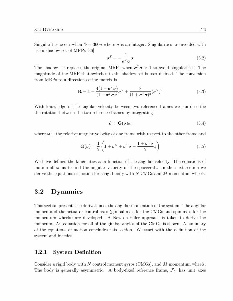
Figure 3.1: System with CMGs and Momentum Wheels
defined by (~b1, ~b2, ~b3)(see Figure 3.1). The body is free to rotate in the inertial reference
frame, FI . Each CMG has a reference frame, FGj(j = 1...N), with unit axes (~asj, ~atj, ~agj)
denoted spin, transverse, and gimbal axes, respectively (see Figure 3.2). The origin of
FGjis at the center of mass of the j -th CMG. The vector components of (~asj, ~atj, ~agj)
are assumed to be given in Fb. The unit vector ~agj is in the direction of the CMG gimbal
axis and fixed in Fb. The flywheel rotates at a constant relative velocity about the spin
axis which is orthogonal to the gimbal axis. The transverse axis is orthogonal to the
gimbal and spin axes. We denote the gimbal angle of the j -th CMG as δj. Given some
initial gimbal angle, δj0, the spin and transverse axes are
~asj(t) = cos(δj(t)− δj0)~asj(0)− sin(δj(t)− δj0)~atj(0) (3.6)
~atj(t) = sin(δj(t)− δj0)~asj(0) + cos(δj(t)− δj0)~atj(0) (3.7)
Using this notion we define a 3×N matrix, As, whose columns are ~asj such that
As = [~as1, ~as2, ..., ~asN ] (3.8)
Matrices At and Ag are defined in the same manner. The gimbal orientation matrix
Ag is constant, while As and At vary with gimbal angles. The relative angular velocity
of the j -th flywheel to its gimbal frame is Ωj~asj. An N × 1 matrix Ω is formed as
[Ω1, Ω2, ..., ΩN ]T . The angular velocity of FGjrelative to Fb is δj~agj. A matrix δ is
formed as [δ1, δ2, ..., δN ]T .
The momentum wheels are defined in a similar manner as the CMGs. Each momentum
wheel has a reference frame FWk(k = 1...M) whose 3 axis aligns with the spin axis. The
spin axis and thus the 3 axis of FWkis fixed in the body. The vector components of the
unit axes (~csk,~ctk,~cgk) are assumed to be given in Fb. We define a matrix
Cs = [~cs1,~cs2, ...,~csM ] (3.9)
3.2 Dynamics 14
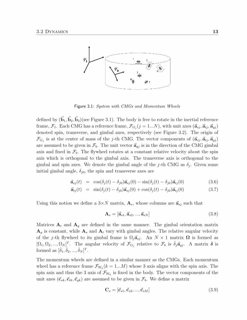
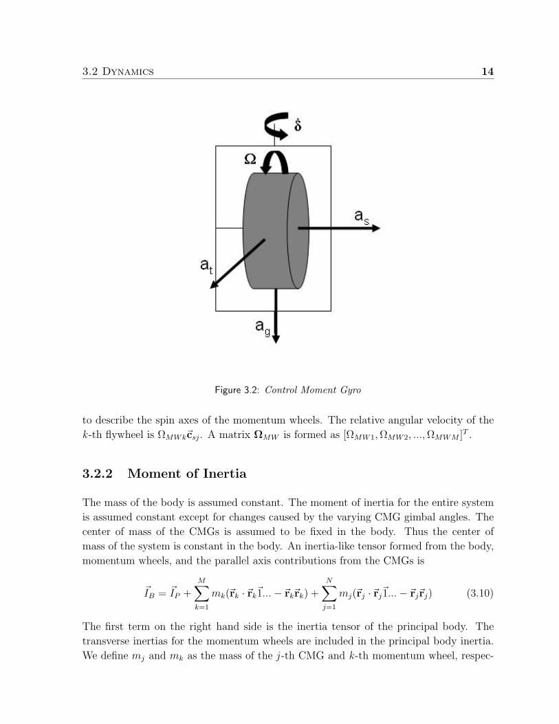
Figure 3.2: Control Moment Gyro
to describe the spin axes of the momentum wheels. The relative angular velocity of the
k -th flywheel is ΩMWk~csj. A matrix ΩMW is formed as [ΩMW1, ΩMW2, ..., ΩMWM ]T .
3.2.2 Moment of Inertia
The mass of the body is assumed constant. The moment of inertia for the entire system
is assumed constant except for changes caused by the varying CMG gimbal angles. The
center of mass of the CMGs is assumed to be fixed in the body. Thus the center of
mass of the system is constant in the body. An inertia-like tensor formed from the body,
momentum wheels, and the parallel axis contributions from the CMGs is
~IB = ~IP +M∑
k=1
mk(~rk ·~rk~1...−~rk~rk) +
N∑j=1
mj(~rj ·~rj~1...−~rj~rj) (3.10)
The first term on the right hand side is the inertia tensor of the principal body. The
transverse inertias for the momentum wheels are included in the principal body inertia.
We define mj and mk as the mass of the j -th CMG and k -th momentum wheel, respec-
3.2 Dynamics 15
tively. The vector from the center of mass of the system to the center of mass of the j -th
CMG is ~rj. The vector from the center of mass of the system to the center of mass of
the k -th momentum wheel is ~rk.
The inertia of the j -th CMG in FGj can be expressed as diag(Isj, Itj, Igj) where Isj, Itj,
Igj represent the spin axis inertia, transverse inertia, and gimbal axis inertia. Note that
the frame inertias are included. We wish to separate the inertia of the flywheel from the
inertia of the frame in the spin axis. We set Isj = Iswj + Isgj where Iswj is the inertia
of the flywheel and Isgj is the inertia of the CMG frame and motor about the spin axis.
We form a matrix
Isw = diag(Isw1, Isw2, ..., IswN) (3.11)
along with three more matrices Isg, It, and Ig which are formed in the same manner.
We form an additional matrix like the CMG flywheel inertia matrix for the momentum
wheels, IswMW = diag(IswMW1, IswMW2, ..., IswMWM). We represent the total inertia of
the system in FB as
I = IB + As(Isw + Isg)ATs + AtItA
Tt + AgIgA
Tg + CsIswMWCT
s (3.12)
where IB represents the tensor from Equation 3.10 in the body-fixed reference frame.
The inertias of the body, and the actuators have been defined. We use the inertias to
find the angular momentum of the system.
3.2.3 Angular Momentum
We assume that the center of mass of the system is an inertial origin. The angular
momentum of the body about its center of mass is
~h = ~IP · ~ω +N∑
j=1
~hCMGja +M∑
k=1
~hMWka (3.13)
where ~hCMGja and ~hMWka are the absolute angular momenta of the j -th CMG and the
k -th MW about their own center of mass, respectively. The absolute angular velocity of
FB is ~ω. The inertia of the whole system is ~I. The absolute angular momentum of the
j -th CMG is defined by~hCMGja = ~Ij · ~ωGji (3.14)
where ~Ij is the inertia tensor of the j -th CMG. The absolute angular velocity of FGj
is ~ωGji. Recall the assumption that the center of mass of the CMG is constant in FB.
Expressed in the body-fixed frame the absolute angular momentum of the j -th CMG is
hCMGja = Ij(ωbi + ωGjb) (3.15)
3.2 Dynamics 16
To simplify notation ω will be the angular velocity of Fb with respect to Fi. We separate
the absolute angular momentum into components in the spin, transverse, and gimbal
directions
hsja = IsjaTsjω + IsjΩj (3.16)
hgja = IgjaTgjω + Igj δj (3.17)
htja = ItjaTtjω (3.18)
The absolute angular momentum of the spin axis of the j -th CMG is split into
hsja = hswja + hsgja (3.19)
where hswa represents the absolute angular momentum of the flywheel about the spin
axis, and hsga the absolute angular momentum of the gimbal frame and motor about the
spin axis.
The absolute angular momentum of the k -th MW is defined as
~hkMWa = ~Ik · ~ωWki (3.20)
where ~ωWki is the absolute angular velocity of the momentum wheel. The spin axis
angular momentum of the k -th MW is an M × 1 matrix hswMWka.
The angular momentum of the system in the body-fixed frame is
h = IBω + Ashsa + Athta + Aghga + CshsMWa (3.21)
where we define hsa = [hs1a, ..., hsNa]T . We define hta, hga, and hsMWa in the same
manner.
We write the absolute angular momentum of the actuators as the sum of the angular
momentum due to the body’s angular velocity and the actuator’s relative angular velocity.
hswa = IswATs ω + hswr (3.22)
hsga = IsgATs ω + hsgr (3.23)
hta = ItATt ω + htr (3.24)
hga = IgATg ω + hgr (3.25)
hswMWa = IswMWCTs ω + hswMWr (3.26)
Notice that the CMGs are constrained to 2 degrees of freedom with respect to the body,
gimbal angle and flywheel spin, therefore
hsgr = htr = 0 (3.27)
3.2 Dynamics 17
The total angular momentum simplifies to
h = (IB + AtItATt + AsIsgA
Ts )ω + Ashswa + Aghga + CshswMWa (3.28)
The end goal is to determine equations that govern the angular momentum of the body
along with the angular momenta of the components of each CMG and momentum wheel.
An equation for the gimbal angle is also developed. From dynamics we know that the
absolute time derivative of any vector ~x in the inertial frame can be defined by the time
derivative of ~x in some frame FP plus the angular velocity of FP with respect to the
inertial frame crossed with the vector ~x. That is,[d~x
dt
]i
=
[d~x
dt
]P
+ ~ω× ~x (3.29)
The absolute time derivative of angular momentum in the inertial frame is
~h = ~v × ~p + ~ge (3.30)
where ~v and ~p are the linear velocity and momentum, respectively. The external torques
on the system are ~ge. Recall the assumption that the center of mass of the system is
translationally fixed in inertial space, therefore ~p = 0. The change in angular momentum
can be expressed in Fb as
h = −ω×h + ge (3.31)
where the superscript × refers to the skew symmetric matrix of the vector such as
ω× =
0 −ω3 ω2
ω3 0 −ω1
−ω2 ω1 0
(3.32)
We have defined the the angular momentum of the system. We now develop the equations
to describe the actuators. The torque inputs to the actuators are the control inputs for
the system. We start with the CMG gimbal angles.
3.2.4 Gimbal Angles
To develop the gimbal angles we start by substituting
hgr = IgjaTg ωGjb = Igj δj (3.33)
3.2 Dynamics 18
into the absolute angular momentum of the CMG about the gimbal axis Equation 3.25.
From the absolute gimbal angular momentum we have an integrable equation for gimbal
angle that is
δj = I−1gj hgja − aT
g ω (3.34)
A general way to write all N integrable equations for gimbal angles is
δ = I−1g hga −AT
g ω (3.35)
With an equation for gimbal angle defined we form matrices ∆c and ∆s where
∆c = diag(cos δ) (3.36)
∆s = diag(sin δ) (3.37)
where cos δ and sin δ are the cosine and sine of the of each term in δ. The initial gimbal
matrices are defined as As0 and At0. These matrices represent As and At when the
gimbal angles are at δj0. As a function of gimbal angle As and At are
As = As0∆c + At0∆
s (3.38)
At = −As0∆s + At0∆
c (3.39)
The time rate of change of As and At is
As = Atdiag(δ) (3.40)
At = −Asdiag(δ) (3.41)
The gimbal angles for all N CMGs have been defined. The CMG control input changes
the gimbal angle. We develop the gimbal momenta to define the control input to the
CMG.
3.2.5 Gimbal Momenta
We want to develop an equation that describes the gimbal angular momentum of the
j -th CMG. The gimbal axis is the control axis for the CMGs. The gimbal axis torque is
ggj = ~agj · ~gCMGj (3.42)
where ~gCMGj is the torque that the body exerts on the j -th CMG. We see that the
absolute angular momentum of the j -th CMG about the gimbal axis is
hgja = ~agj · ~hCMGj (3.43)
3.2 Dynamics 19
The time derivative of hgja is
hgja = ~agj · ~hCMGj + ggj (3.44)
where the time derivative of the unit vector ~agj is
~agj = ~ω× ~agj (3.45)
Using the vector identity (~a× ~b) · ~c = ~a · (~b× ~c), equation 3.44 can be rewritten as
hgja = ~ω · (~agj × ~hCMGj) + ggj (3.46)
We separate the gimbal and wheel angular momenta
~hCMGj = ~Igj · ~ωGji +~Iwj · (~ωGji + [Ωj, 0, 0]T ) (3.47)
where
~ωGji = δj~agj + ~ω (3.48)
~Iwj = Itj~1 + (Isj − Itj)~asj~asj (3.49)
Substituting into equation 3.46 leads to
hgja = ~ω · (~agj × (~Iwj · (Ωj~asj + δj~agj + ~ω) +~Ig · (δ~ag + ~ω))) + ggj (3.50)
which we can integrate to find the absolute angular momentum of the gimbal axis of the
j -th CMG.
To expand this equation for all gimbal angular momenta we write
hga = ~ω · (~Ag × (Ω~As + δ~Ag + ~ω) +~Ig · (δ~Ag + ~ω)) + gg (3.51)
This equation can be simplified as shown in Ref. [4] to
hga = diag((It − Isg)ATs ω− hswa)(A
Tt ω) + gg (3.52)
The equation for the CMGs gimbal axis angular momentum provides a useful means of
implementing control by keeping the gimbal axis torque term separate.
3.2.6 Spin Momenta
We define in order to find an equation that governs the flywheel spin axis momentum
g = ~cs · ~gw (3.53)
3.2 Dynamics 20
where ~gw is the torque that the body imparts on the flywheel. The scalar gMW represents
the axial torque on the flywheel. The absolute angular momentum of any flywheel in the
~cs direction is
hswa = ~cs · ~hwa (3.54)
where ~hwa is the absolute angular momentum of the flywheel. Differentiating gives
hswa = ~cs · ~hswa + ~cs · ~hswa (3.55)
The time derivative of the unit vector ~cs is
~cs = ~ω× ~cs (3.56)
The change in angular momentum of the flywheel can be rewritten as
hswa = (~ω× ~cs) · ~hswa + ~cs · ~hswa (3.57)
= ~ω · (~cs × ~hswa) + ~cs · ~gw (3.58)
= ~ω · ~cs ×~Isw · ~ωwa + g (3.59)
where
~ωwa = ~ω + Ω~cs (3.60)
is the absolute angular velocity of the flywheel. We write the flywheel inertia dyadic as
~Isw = It~1 + (Is − It)~cs~cs (3.61)
where It and Is are the transverse and spin inertias of the flywheel. Using the previous
two equations we can form the following equalities [6]
~ω · ~cs × ~ωwa = 0 (3.62)
~cs ×~Isw = It~csj × ~1 (3.63)
Equation 3.59 simplifies to describe the motion of the flywheel as
hswa = g (3.64)
We use the subscript MW to denote equations that describe the momentum wheels.
hswMWa = gMW (3.65)
for all M momentum wheels.
3.3 Summary 21
3.3 Summary
We have presented all 6 + 2N + M equations necessary to describe the motion of a rigid
body with N CMGs and M momentum wheels. They are
h = −ω×h + ge (3.66)
hswMWa = gMW (3.67)
hga = diag((It − (Isg + Isw))ATs ω− IswΩ)(AT
t ω) + gg (3.68)
δ = I−1g hga −AT
g ω (3.69)
σ = G(σ)ω (3.70)
where
h = (IB + AtItATt + AsIsgA
Ts )ω + Ashswa + Aghga + CshswMWa (3.71)
hswa = IswATs ω + IswΩ (3.72)
hga = IgATg ω + Igδ (3.73)
hswMWa = IswMWCTs ω + IswMWΩMW (3.74)
(3.75)
Equation 3.66 describes the angular momentum of the system. Equations 3.67 & 3.68
are the control axes for the momentum wheel and CMG, respectively. The CMG gimbal
angles are represented in Equation 3.69. The kinematics for the body-fixed reference
frame to the inertia reference frame are described by Equation 3.70. The equations of
motion are used in the derivations of control laws.
22
Chapter 4
Controllers
We wish to derive control strategies and control laws that will drive the spacecraft along a
reference motion. This chapter presents two control strategies. The purpose of the control
strategies is to take advantage of the torque amplification of the CMGs by allowing the
CMGs to provide the majority of the torque required for a given reorientation. The
momentum wheels correct for initial condition and tracking errors. Control Strategy I
uses the CMGs in open loop control to drive the spacecraft about a reference path, with
the momentum wheels implementing a closed loop control law to correct for tracking
errors. The momentum wheel control laws are derived through Lyapunov and feedback
linearization techniques. Control Strategy II uses both the CMGs and momentum wheels
in closed loop control. A control approach that uses both types of actuators in parallel is
presented. A pseudo-parallel control strategy that uses a CMG closed loop controller and
Euler integration of the state errors to provide a momentum wheel feedforward control
law is presented.
The chapter begins with a brief review of Lyapunov and feedback linearization control
techniques. A definition of the desired maneuver follows. The tracking errors, which
are the control states, are defined next. We review the gimbal rate steering law and
singularity robust modification of Oh and Vadali [12]. We discuss Singularity Direction
Avoidance presented in Refs. [4, 16] which is an improved singularity avoidance gimbal
rate steering law. Discussion of the control strategies and derivation of the momentum
wheel feedback control laws conclude the chapter.
4.1 Nonlinear Control Techniques 23
4.1 Nonlinear Control Techniques
Methods for linearly controlling a nonlinear system, such as linearization of the dynam-
ics, can perform effectively. However, the benefits of considering the nonlinear dynamics
can include increased robustness, control over a larger envelope of the dynamics, control
of linearly uncontrollable systems, and preservation of physical insight into the prob-
lem. Thus, we consider nonlinear control techniques. The nonlinear control techniques,
Lyapunov Direct and Feedback Linearization, are briefly reviewed.
4.1.1 Lyapunov Control Laws
The derivation of a Lyapunov control law is based on Lyapunov’s second method. Con-
sider a set of differential equations x = f(x) which describe a dynamic system. The state
x = y − yd is the difference between the desired and current state. The stability of the
system is analyzed by examining a scalar energy-like function of the state, V = V (x).
The desired state is globally asymptotically stable if
V (0) = 0 (4.1)
V (x) > 0 for x 6= 0 (4.2)
V (x) → ∞ for ‖x‖ → ∞ (4.3)
V (x) < 0 for x 6= 0 (4.4)
Lyapunov control laws use the inputs of the system to ensure that the conditions for
stability of the desired state are met. [37, 38]
4.1.2 Feedback Linearization
The purpose of feedback linearization is to use the inputs to cancel out the nonlinearities
of the system. Linear feedback control laws can then be applied to the system to provide
stability. For a continuously differentiable system x = f(x,u), where f(0,0) = 0, we
want to use a state feedback controller that stabilizes the system. Note that for a system
in the standard feedback linearization form,
x = Ax + Bβ−1(x)[u− α(x)] (4.5)
we can choose a control,
u = α(x) + β(x)ν (4.6)
4.2 Reference Motion 24
that makes the closed loop dynamics,
x = Ax + Bν (4.7)
linear. By setting ν = Kx, and choosing gain K such that A+BK is Hurwitz, the closed
loop system is made globally asymptotically stable. Systems that are not in the standard
form can be transformed with a change of state variables since the state equations of the
system are not unique. Details on the state variable transformation can be found in
Refs. [37, 38, 39].
4.2 Reference Motion
We now define the motion that we want the spacecraft to track. Consider a rigid reference
body that has a body-fixed reference frame FR. The center of mass of the reference body
is coincident with the origin of FR and is fixed in inertial space. The orientation of FR
with respect to the inertial reference frame FI is expressed by the direction cosine matrix
RRI and by a set of MRPs, σR. The equations that describe the motion of the reference
body are
hR = −ω×RIBωR + gR (4.8)
σR = G(σR)ωR (4.9)
where ωR is the absolute angular velocity of FR and gR is the external torque on the
reference body. Note that the reference body has the same inertia as the controlled body
but does not include the actuator inertias.
4.3 Error States
With the reference body and the spacecraft fully defined we can form the terms δσ and
δω [40],
δσ = σ− σR (4.10)
=(1− σT
RσR)σ− (1− σT σ)σR + 2σ×σR
1 + (σTRσR)(σT σ) + 2σT
Rσ(4.11)
δω = ω−RBRωR (4.12)
Using these equations we define
δh = h− IBRBRωR (4.13)
4.4 Control Moment Gyro Feedback Control Law 25
the difference between the angular momentum of the bodies, where RBR = R(δσ).
Substituting Equation 3.28 into δh and simplifying gives
δh = IBω + (AtItATt + AsIsgA
Ts )ω + Ashswa + Aghga (4.14)
+CshswMWa − IBRBRωR
= IBδω + (AtItATt + AsIsgA
Ts )ω + Ashswa + Aghga (4.15)
+CshswMWa
Taking the time derivative of Equation 4.13 yields
δh = h− IBdRBR
dtωR − IBRBRωR (4.16)
Hall et al. [2] showed that
IBdRBR
dtωR = IBω×δω (4.17)
Taking the time derivative of Equation 4.15 gives
δh = IBδω + Ashswa + Ashswa + Aghga + CshswMWa (4.18)
+(AtItATt + AtItA
Tt + AsIsgA
Ts + AsIsgA
Ts )ω + (AtItA
Tt + AsIsgA
Ts )ω
The state equations are the attitude and angular velocity error rates. We use Equa-
tion 4.18 and Equation 3.4 to express the states as
δσ = G(δσ)δω (4.19)
δω = I−1B [δh− Ashswa −Ashswa −Aghga − (AtItA
Tt + AsIsgA
Ts )ω (4.20)
−(AtItATt + AtItA
Tt + AsIsgA
Ts + AsIsgA
Ts )ω−CsgMW ]
The state equations are time invariant.
The error between the reference frame motion and the body-fixed motion has been de-
fined. We use the tracking error as the states of our nonlinear control laws. The remainder
of the chapter focuses on control laws that drive the tracking error to zero.
4.4 Control Moment Gyro Feedback Control Law
We use a gimbal rate steering law first presented by Oh and Vadali [12] to find the CMG
control maneuver for a large rapid slew. Presented in this notation the gimbal torques
are
gg = Igδ + IgATg ω− diag((It − Is)A
Ts ω− IswΩ)AT
t ω (4.21)
4.4 Control Moment Gyro Feedback Control Law 26
where
δ = kδ(δdes − δ) (4.22)
δdes = D†(k3δω + k4δσ− IBRBRωR − I−1B ω×(IBω + Ashswa + Aghga)) (4.23)
D = −Atdiag(IswΩ) (4.24)
+1/2[(as1aTt1 + at1a
Ts1)(ω + RBRωR) (as2a
Tt2 + at2a
Ts2)(ω + RBRωR)...
...(asNaTtN + atNaT
sN)(ω + RBRωR)](It − Is)
The † denotes the pseudo-inverse. The coefficients kδ, k3, and k4 are positive constant
scalars [4].
4.4.1 Singularity Avoidance
Special configurations of the CMG gimbal angles can result in singularities where the
CMG cluster cannot provide torque in a specified direction. To avoid singular configura-
tions we use a singularity-robust steering law [12]. For simplicity we rewrite equation 4.23
as
δdes = D†Lr (4.25)
Unreasonable gimbal rates are produced when D becomes close to singular. We modify
equation 4.25 to be
δdes = DT (DDT + α1)−1Lr (4.26)
where
α = α0 exp− det(DDT ) (4.27)
is a scalar parameter that increases as a singularity configuration is approached. The
coefficient α0 is a small constant [12].
4.4.2 Singular Direction Avoidance
An improvement to singularity-robust steering law [12] called Singular Direction Avoid-
ance was presented by Ford and Hall [4, 16]. Singular Direction Avoidance is based on
the singular value decomposition to compute the pseudo inverse in order to steer the
CMGs away from singular configurations. Ford and Hall proved that the torque error
from singularity avoidance was always less with Singular Direction Avoidance than with
singularity-robust steering law [4, 16].
We modify Equation 4.27 to be
α = α0 exp−kSDAσ233 (4.28)
4.5 Control Strategy I: Open Loop Control Moment Gyro with ClosedLoop Momentum Wheel Control 27
where
σ233 =
√3/NS(3, 3)/hswr (4.29)
The number of CMGs in the spacecraft is N . The matrix S is found through the singular
value decomposition problem. For the general m× n matrix D can be decomposed into
a product of three matrices
D = USVT (4.30)
where U is an m ×m unitary matrix,V is an n × n unitary matrix, and S is an m × n
diagonal matrix. Equation 4.26 becomes
δdes = VSUT Lr (4.31)
where
S = diag(1/S11, 1/S22, S33/(S233 + α)) (4.32)
We perform numerical simulations of Singular Direction Avoidance versus singularity-
robust to illustrate its benefits. For the majority of the simulations that involve mixed
attitude control strategies we use the singularity-robust steering law.
4.5 Control Strategy I: Open Loop Control Moment
Gyro with Closed Loop Momentum Wheel Con-
trol
The first strategy requires prerequisite knowledge of the reorientation or reference mo-
tion. Numerical simulation of the CMG gimbal rate steering law for the given reference
motion are performed. The gimbal angle, velocity, and acceleration for the maneuver
are found from the numerical simulation. The gimbal information is implemented on the
spacecraft in an open loop form. With zero initial condition error and perfect knowl-
edge of the system the open loop CMG maneuver will force the spacecraft along the
desired reference motion. However, initial condition errors, perturbations, and/or sys-
tem parameter uncertainty will cause the spacecraft to diverge from the reference motion.
Implementation of the derived momentum wheel feedback control laws correct for initial
condition errors and perturbations. Figure 4.1 shows a block diagram of the control strat-
egy. The ‘Reference Motion’ block symbolizes the angular velocity and attitude for the
desired maneuver. The ‘System’ block represents the spacecraft’s angular velocity and
attitude. The output of the system is the difference between the reference and system
angular velocity and attitude. The CMG gimbal information from the preprocessed ma-
neuver is passed to the spacecraft in open loop. The momentum wheel feedback control
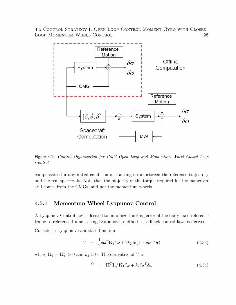
4.5 Control Strategy I: Open Loop Control Moment Gyro with ClosedLoop Momentum Wheel Control 28
Figure 4.1: Control Organization for CMG Open Loop and Momentum Wheel Closed LoopControl
compensates for any initial condition or tracking error between the reference trajectory
and the real spacecraft. Note that the majority of the torque required for the maneuver
still comes from the CMGs, and not the momentum wheels.
4.5.1 Momentum Wheel Lyapunov Control
A Lyapunov Control law is derived to minimize tracking error of the body fixed reference
frame to reference frame. Using Lyapunov’s method a feedback control laws is derived.
Consider a Lyapunov candidate function
V =1
2δωTK1δω + 2k2 ln(1 + δσT δσ) (4.33)
where K1 = KT1 > 0 and k2 > 0. The derivative of V is
V = HT I−1B K1δω + k2δσT δω (4.34)
4.5 Control Strategy I: Open Loop Control Moment Gyro with ClosedLoop Momentum Wheel Control 29
where
H = δh− Ashswa −Ashswa −CshswMWa −Aghga (4.35)
−(AtItATt + AtItA
Tt + AsIsgA
Ts + AsIsgA
Ts )ω
−(AtItATt + AsIsgA
Ts )ω
Equation 4.35 can be expanded to
H = −ω×((IB + AtItATt + AsIsgA
Ts )ω + Ashswa + Aghga (4.36)
+CshswMWa) + ge − IBω×δω− IBRBRI−1B [−ω×RIωR + gR]
−Ashswa −Asgw −CsgMW
−Ag(diag((It − Is)ATs ω− IswΩ)(AT
t ω) + gg)
−(AtItATt + AtItA
Tt + AsIsgA
Ts + AsIsgA
Ts )ω
−(AtItATt + AsIsgA
Ts )ω
With H in expanded form we identify the control torques for the system ge, gw, gg, and
gMW . The spin torque for a CMG to maintain a constant velocity of the flywheel about
its spin axis relative to the body is
gw = Isw(ATs ω + AT
s ω) (4.37)
For this problem we consider ge, gw, and gg as known parameters. With the gMW input
we can insure that the conditions for global asymptotic stability, Equations 4.1, 4.2, 4.3, 4.4,
are met.
By choosing K1 = IB equation 4.34 becomes
V = δωT (H + k2δσ) (4.38)
We choose the control torque gMW to be
CsgMW = δh− Ashswa −Asgw −Aghga − (AtItATt + AsIsgA
Ts )ω (4.39)
−(AtItATt + AtItA
Tt + AsIsgA
Ts + AsIsgA
Ts )ω
+k2δσ + k1δω
which yields
V = −k1δωT δω ≤ 0 (4.40)
since k1 > 0. From this result we see that
limt→∞
δω(t) = 0 (4.41)
4.5 Control Strategy I: Open Loop Control Moment Gyro with ClosedLoop Momentum Wheel Control 30
Substituting the control input Equation 4.39 into the state equation δω, we have
IBδω = −k2δσ− k1δω (4.42)
Due to Equation 4.41 we have
limt→∞
IBδω = − limt→∞
k2δσ (4.43)
so that δσ → 0. From Equation 4.19 we know that δσ → 0, therefore the limit of δσ is
a constant, thus
limt→0
δσ = 0 (4.44)
With LaSalle’s Invariance Principle [37], the attitude and angular velocity error due to
tracking with this control law is globally asymptotically stable.
4.5.2 Momentum Wheel Lyapunov Control with Constant Mo-
ment of Inertia Assumption
For most systems the change in inertia due to the CMGs is orders of magnitude smaller
than the system inertia. We can reduces the amount of computation required by the
controller if we assume that the change in the moment of inertia of the system due to
the CMGs is negligible. The state equations are
δσ = G(δσ)δω (4.45)
δω = I−1B [δh− Ashswa −Ashswa −Aghga − (AtItA
Tt + AsIsgA
Ts )ω (4.46)
−CsgMW ]
Using the Lyapunov candidate function of Equation 4.33 a control input of
CsgMW = δh− Ashswa −Asgw −Aghga − (AtItATt + AsIsgA
Ts )ω (4.47)
+k2δσ + k1δω
globally asymptotically stabilizes the desired state.
4.5.3 Momentum Wheel Lyapunov Control Without Knowl-
edge of the CMGs
To save computation time we consider the previous Lyapunov control laws without knowl-
edge of the CMGs. Equation 4.18 becomes
δh = IBδω + CshswMWa (4.48)
4.5 Control Strategy I: Open Loop Control Moment Gyro with ClosedLoop Momentum Wheel Control 31
The time derivative of the angular velocity error Equation 4.20 becomes
δω = I−1B [δh−CsgMW ] (4.49)
The candidate Lyapunov function remains in the same form as Equation 4.33 where
K1 = KT1 > 0 and k2 > 0. The time derivative of the candidate Lyapunov function is
V = δωT (δh−CshswMWa + k2δσ) (4.50)
where we have chosen K1 = IB. Clearly by choosing
CsgMW = δh + k2δσ + k1δω (4.51)
the system will be globally asymptotically stable given the previous LaSalle’s Invariance
Principal discussion.
4.5.4 Momentum Wheel Feedback Linearization
We now take a different approach to feedback control. For a certain class of nonlinear
systems we can use a change of variables and state feedback control that transforms the
nonlinear system into a linear system [37]. We investigate input-state linearization of
this nonlinear system.
We begin with the state equations 4.19 and 4.20 which we transform with
z1 = δσ (4.52)
z2 = G(δσ)δω = δσ (4.53)
The transformed state equations are
z1 = z2 (4.54)
z2 = Gδω + Gδω (4.55)
where G = G(δσ). Substitution of Equation 4.20 allows the state equations to be written
as
z1 = z2 (4.56)
z2 = Gδω + G(I−1B (δh− Ashswa −Ashswa −Aghga (4.57)
−(AtItATt + AtItA
Tt + AsIsgA
Ts + AsIsgA
Ts )ω
−(AtItATt + AsIsgA
Ts )ω−CsgMW )
4.5 Control Strategy I: Open Loop Control Moment Gyro with ClosedLoop Momentum Wheel Control 32
In this form we can choose CsgMW to cancel the nonlinear terms. We choose the mo-
mentum wheel control torques to be
CsgMW = δh− Ashswa −Ashswa −Aghga (4.58)
−(AtItATt + AtItA
Tt + AsIsgA
Ts + AsIsgA
Ts )ω
−(AtItATt + AsIsgA
Ts )ω + IBG−1(Gδω + ν)
where
ν = k5δω + k6δσ (4.59)
The constants k5 and k6 are positive. The system with control is
z =
[k6 0
0 k5G−1
]z (4.60)
With the linear closed loop system we can use linear stability analysis. From linear theory
we can guarantee asymptotic stability if the coefficient matrix is Hurwitz[37].
4.5.5 One Open Loop CMG and Momentum Wheel Feedback
Control
We now consider using one CMG to provide large torques about a single axis, while a
cluster of momentum wheels provide closed loop attitude control. Any of the previously
derived closed loop momentum wheel control laws can be used in this configuration since
the stability of the closed loop system comes from the momentum wheel control laws.
The advantage of this configuration is in the savings in physical hardware. The spacecraft
would not require the typical 3 or 4 CMG cluster for attitude control.
Since there is an open loop portion of the controller, prior knowledge of the reference
motion is still required. The calculation of the open loop CMG commands can be sim-
plified. The desired output torque from the CMG is about the transverse axis. The
output torque is IswΩ sin δ/∆t, where ∆t is the time to complete the gimbal angle. A
more detailed discussion of the CMG output torque is in Chapter 6.
For a given reference motion we choose the CMG maneuver such that the output torque
of the CMG provides much of the required torque for tracking. A simple example is
to use the CMG to provide torque for a principal axis slew of the spacecraft, while
the momentum wheel correct for the tracking errors. We use this example and actuator
configuration on the spacecraft simulator. The simulator results are presented in Chapter
6.
4.6 Control Strategy II: Control Moment Gyro and Momentum WheelClosed Loop Control 33
4.6 Control Strategy II: Control Moment Gyro and
Momentum Wheel Closed Loop Control
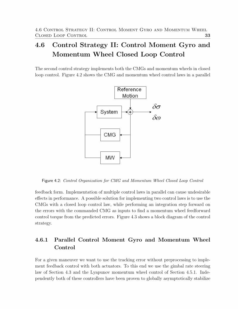
The second control strategy implements both the CMGs and momentum wheels in closed
loop control. Figure 4.2 shows the CMG and momentum wheel control laws in a parallel
Figure 4.2: Control Organization for CMG and Momentum Wheel Closed Loop Control
feedback form. Implementation of multiple control laws in parallel can cause undesirable
effects in performance. A possible solution for implementing two control laws is to use the
CMGs with a closed loop control law, while performing an integration step forward on
the errors with the commanded CMG as inputs to find a momentum wheel feedforward
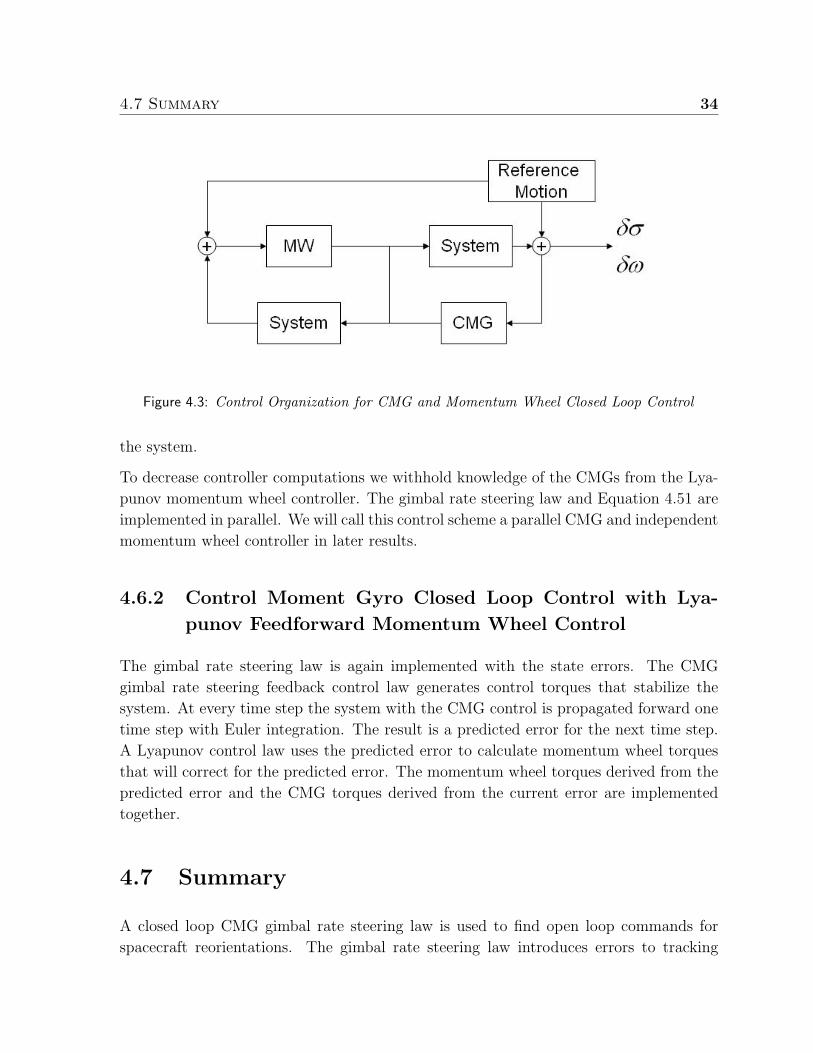
control torque from the predicted errors. Figure 4.3 shows a block diagram of the control
strategy.
4.6.1 Parallel Control Moment Gyro and Momentum Wheel
Control
For a given maneuver we want to use the tracking error without preprocessing to imple-
ment feedback control with both actuators. To this end we use the gimbal rate steering
law of Section 4.3 and the Lyapunov momentum wheel control of Section 4.5.1. Inde-
pendently both of these controllers have been proven to globally asymptotically stabilize
4.7 Summary 34
Figure 4.3: Control Organization for CMG and Momentum Wheel Closed Loop Control
the system.
To decrease controller computations we withhold knowledge of the CMGs from the Lya-
punov momentum wheel controller. The gimbal rate steering law and Equation 4.51 are
implemented in parallel. We will call this control scheme a parallel CMG and independent
momentum wheel controller in later results.
4.6.2 Control Moment Gyro Closed Loop Control with Lya-
punov Feedforward Momentum Wheel Control
The gimbal rate steering law is again implemented with the state errors. The CMG
gimbal rate steering feedback control law generates control torques that stabilize the
system. At every time step the system with the CMG control is propagated forward one
time step with Euler integration. The result is a predicted error for the next time step.
A Lyapunov control law uses the predicted error to calculate momentum wheel torques
that will correct for the predicted error. The momentum wheel torques derived from the
predicted error and the CMG torques derived from the current error are implemented
together.
4.7 Summary
A closed loop CMG gimbal rate steering law is used to find open loop commands for
spacecraft reorientations. The gimbal rate steering law introduces errors to tracking
4.7 Summary 35
by neglecting the effects of gimbal acceleration with the gimbal inertia. With perfect
knowledge of the system the tracking errors are minimal. Momentum wheel closed loop
control laws attempt to reject undesirable gimbal torques and initial condition errors.
Using the CMGs in open loop with prerequisite knowledge of the maneuver can be
restrictive on time and generally impractical for a real spacecraft. The open loop CMG
commands have to be stored in a table which the processor must continually query. Also
the maneuver must be preprocessed in order to calculate the open loop CMG commands.
Under ideal conditions the time lag between receiving a reference motion and execution of
the maneuver might be acceptable. However, the inherit slowness of this strategy might
make it unsuitable for mission goals that require large rapid slewing. A possible solution
is to simplify the preprocessing by reducing the number of CMGs. Aligning the output
torque of a single CMG to provide large slew torques with momentum wheel feedback
can reduce time lag.
With use of Euler integration of the system with knowledge of the gimbal control torques
to be applied, the attitude and angular velocity error can be predicted for the next
time step. Lyapunov momentum wheel control uses the predicted error to calculate the
required torques which are implemented in feedforward fashion.
36
Chapter 5
Numerical Simulation
We present the results of numerical simulations of the derived control laws for illus-
tration. We first present the reference motion to be tracked. The CMG gimbal rate
steering law demonstrates convergence without initial condition errors. We then show
how implementing the CMG maneuver from preprocessing with slight variations in initial
conditions make the system diverge (as expected) from the desired reference conditions.
Implementation of the closed loop momentum wheel control laws from Strategy I show
that tracking errors are rejected with minimal torques. Simulation results are shown for
the parallel CMG/independent momentum wheel and the CMG feedback/momentum
wheel feedforward control laws.
A trend analysis is performed to investigate the control effort variation with respect to
the reference slew rate. Two controllers from Control Strategy I and II are evaluated.
A quantification of the control effort required for a maneuver is presented. The control
effort-like-measure is compared for simulations with and without initial condition errors.
Plots of maximum control torques for each maneuver and controller with and without
initial condition errors illustrate the differences between the controllers.
For all the results the time units are seconds. The angular rate units are rad/sec. The
external and control torque units are N ·m.
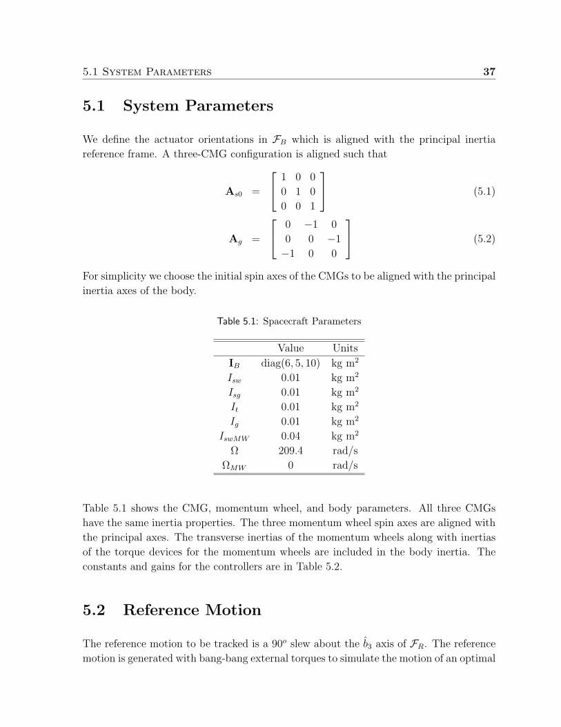
5.1 System Parameters 37
5.1 System Parameters
We define the actuator orientations in FB which is aligned with the principal inertia
reference frame. A three-CMG configuration is aligned such that
As0 =
1 0 0
0 1 0
0 0 1
(5.1)
Ag =
0 −1 0
0 0 −1
−1 0 0
(5.2)
For simplicity we choose the initial spin axes of the CMGs to be aligned with the principal
inertia axes of the body.
Table 5.1: Spacecraft Parameters
Value Units
IB diag(6, 5, 10) kg m2
Isw 0.01 kg m2
Isg 0.01 kg m2
It 0.01 kg m2
Ig 0.01 kg m2
IswMW 0.04 kg m2
Ω 209.4 rad/s
ΩMW 0 rad/s
Table 5.1 shows the CMG, momentum wheel, and body parameters. All three CMGs
have the same inertia properties. The three momentum wheel spin axes are aligned with
the principal axes. The transverse inertias of the momentum wheels along with inertias
of the torque devices for the momentum wheels are included in the body inertia. The
constants and gains for the controllers are in Table 5.2.
5.2 Reference Motion
The reference motion to be tracked is a 90o slew about the b3 axis of FR. The reference
motion is generated with bang-bang external torques to simulate the motion of an optimal
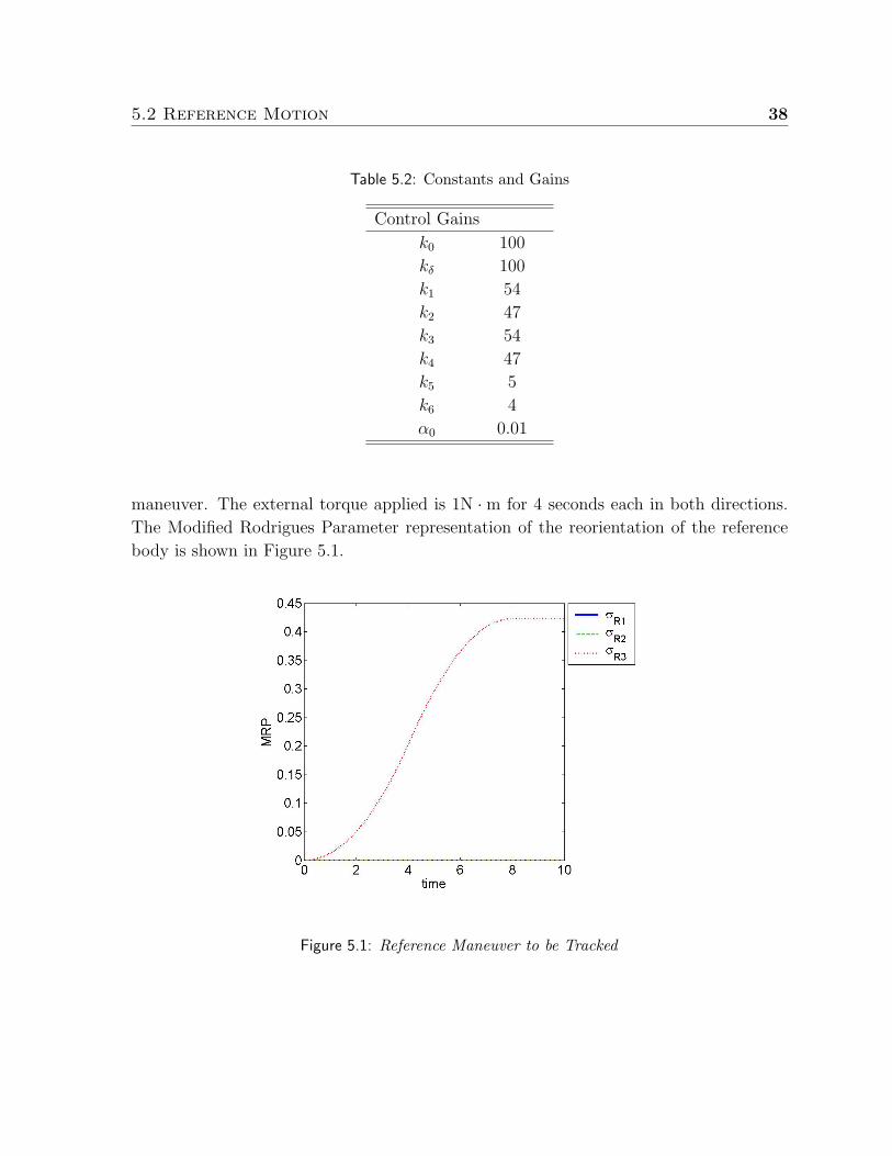
5.2 Reference Motion 38
Table 5.2: Constants and Gains
Control Gains
k0 100
kδ 100
k1 54
k2 47
k3 54
k4 47
k5 5
k6 4
α0 0.01
maneuver. The external torque applied is 1N ·m for 4 seconds each in both directions.
The Modified Rodrigues Parameter representation of the reorientation of the reference
body is shown in Figure 5.1.
Figure 5.1: Reference Maneuver to be Tracked
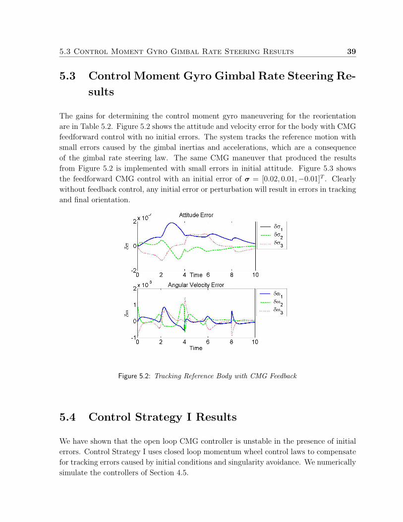
5.3 Control Moment Gyro Gimbal Rate Steering Results 39
5.3 Control Moment Gyro Gimbal Rate Steering Re-
sults
The gains for determining the control moment gyro maneuvering for the reorientation
are in Table 5.2. Figure 5.2 shows the attitude and velocity error for the body with CMG
feedforward control with no initial errors. The system tracks the reference motion with
small errors caused by the gimbal inertias and accelerations, which are a consequence
of the gimbal rate steering law. The same CMG maneuver that produced the results
from Figure 5.2 is implemented with small errors in initial attitude. Figure 5.3 shows
the feedforward CMG control with an initial error of σ = [0.02, 0.01,−0.01]T . Clearly
without feedback control, any initial error or perturbation will result in errors in tracking
and final orientation.
Figure 5.2: Tracking Reference Body with CMG Feedback
5.4 Control Strategy I Results
We have shown that the open loop CMG controller is unstable in the presence of initial
errors. Control Strategy I uses closed loop momentum wheel control laws to compensate
for tracking errors caused by initial conditions and singularity avoidance. We numerically
simulate the controllers of Section 4.5.
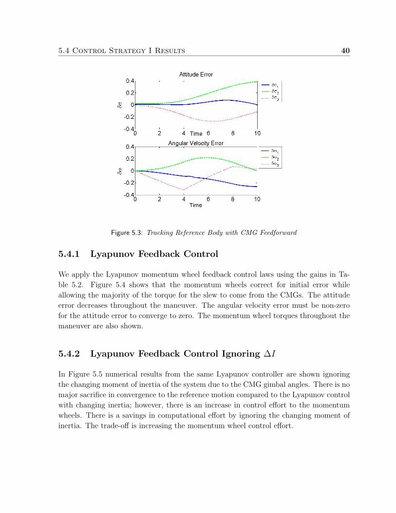
5.4 Control Strategy I Results 40
Figure 5.3: Tracking Reference Body with CMG Feedforward
5.4.1 Lyapunov Feedback Control
We apply the Lyapunov momentum wheel feedback control laws using the gains in Ta-
ble 5.2. Figure 5.4 shows that the momentum wheels correct for initial error while
allowing the majority of the torque for the slew to come from the CMGs. The attitude
error decreases throughout the maneuver. The angular velocity error must be non-zero
for the attitude error to converge to zero. The momentum wheel torques throughout the
maneuver are also shown.
5.4.2 Lyapunov Feedback Control Ignoring ∆I
In Figure 5.5 numerical results from the same Lyapunov controller are shown ignoring
the changing moment of inertia of the system due to the CMG gimbal angles. There is no
major sacrifice in convergence to the reference motion compared to the Lyapunov control
with changing inertia; however, there is an increase in control effort to the momentum
wheels. There is a savings in computational effort by ignoring the changing moment of
inertia. The trade-off is increasing the momentum wheel control effort.
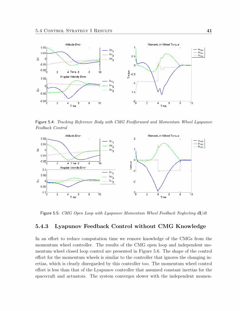
5.4 Control Strategy I Results 41
Figure 5.4: Tracking Reference Body with CMG Feedforward and Momentum Wheel LyapunovFeedback Control
Figure 5.5: CMG Open Loop with Lyapunov Momentum Wheel Feedback Neglecting dI/dt
5.4.3 Lyapunov Feedback Control without CMG Knowledge
In an effort to reduce computation time we remove knowledge of the CMGs from the
momentum wheel controller. The results of the CMG open loop and independent mo-
mentum wheel closed loop control are presented in Figure 5.6. The shape of the control
effort for the momentum wheels is similar to the controller that ignores the changing in-
ertias, which is clearly disregarded by this controller too. The momentum wheel control
effort is less than that of the Lyapunov controller that assumed constant inertias for the
spacecraft and actuators. The system converges slower with the independent momen-
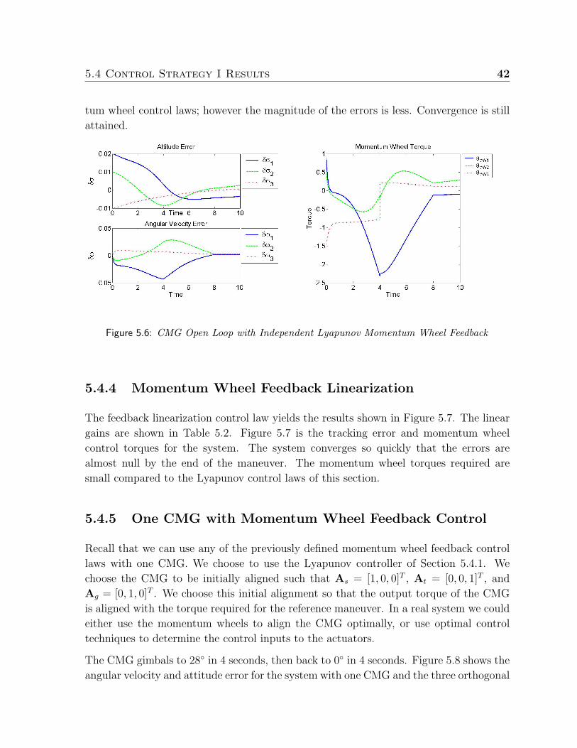
5.4 Control Strategy I Results 42
tum wheel control laws; however the magnitude of the errors is less. Convergence is still
attained.
Figure 5.6: CMG Open Loop with Independent Lyapunov Momentum Wheel Feedback
5.4.4 Momentum Wheel Feedback Linearization
The feedback linearization control law yields the results shown in Figure 5.7. The linear
gains are shown in Table 5.2. Figure 5.7 is the tracking error and momentum wheel
control torques for the system. The system converges so quickly that the errors are
almost null by the end of the maneuver. The momentum wheel torques required are
small compared to the Lyapunov control laws of this section.
5.4.5 One CMG with Momentum Wheel Feedback Control
Recall that we can use any of the previously defined momentum wheel feedback control
laws with one CMG. We choose to use the Lyapunov controller of Section 5.4.1. We
choose the CMG to be initially aligned such that As = [1, 0, 0]T , At = [0, 0, 1]T , and
Ag = [0, 1, 0]T . We choose this initial alignment so that the output torque of the CMG
is aligned with the torque required for the reference maneuver. In a real system we could
either use the momentum wheels to align the CMG optimally, or use optimal control
techniques to determine the control inputs to the actuators.
The CMG gimbals to 28 in 4 seconds, then back to 0 in 4 seconds. Figure 5.8 shows the
angular velocity and attitude error for the system with one CMG and the three orthogonal
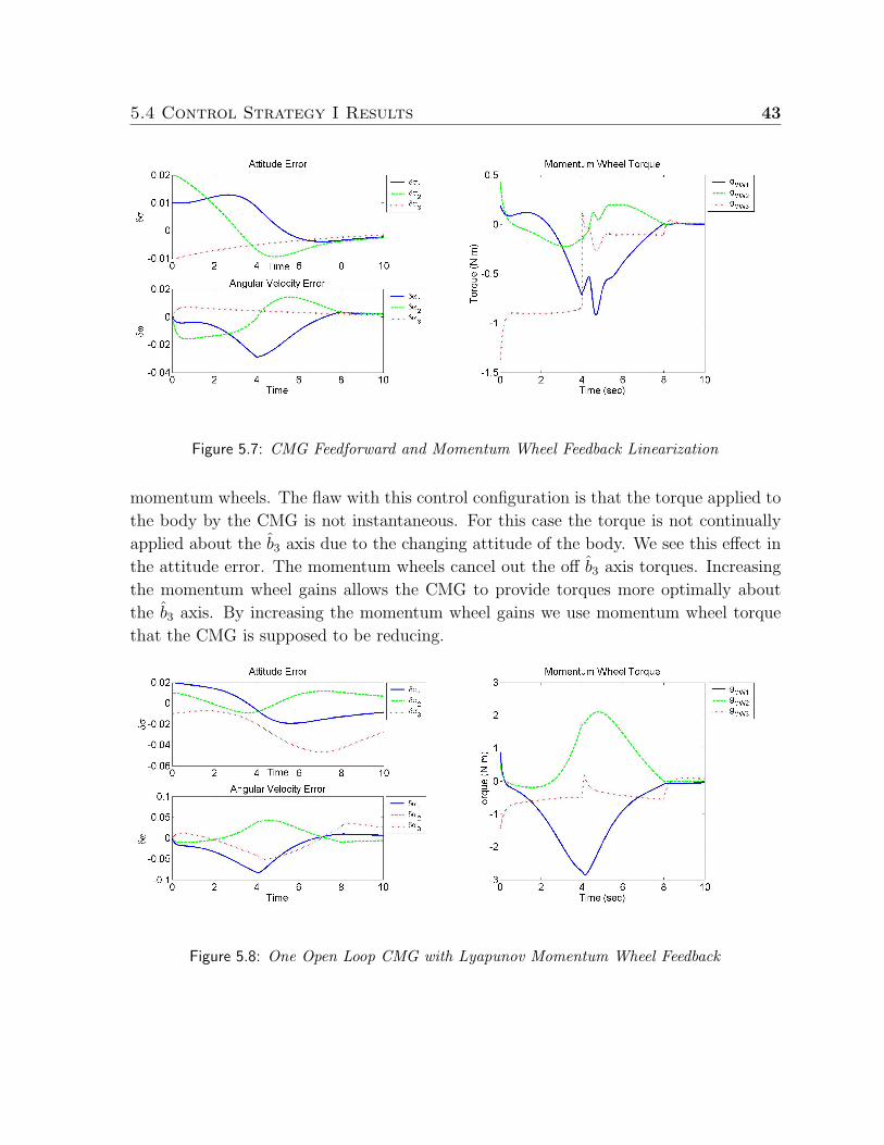
5.4 Control Strategy I Results 43
Figure 5.7: CMG Feedforward and Momentum Wheel Feedback Linearization
momentum wheels. The flaw with this control configuration is that the torque applied to
the body by the CMG is not instantaneous. For this case the torque is not continually
applied about the b3 axis due to the changing attitude of the body. We see this effect in
the attitude error. The momentum wheels cancel out the off b3 axis torques. Increasing
the momentum wheel gains allows the CMG to provide torques more optimally about
the b3 axis. By increasing the momentum wheel gains we use momentum wheel torque
that the CMG is supposed to be reducing.
Figure 5.8: One Open Loop CMG with Lyapunov Momentum Wheel Feedback
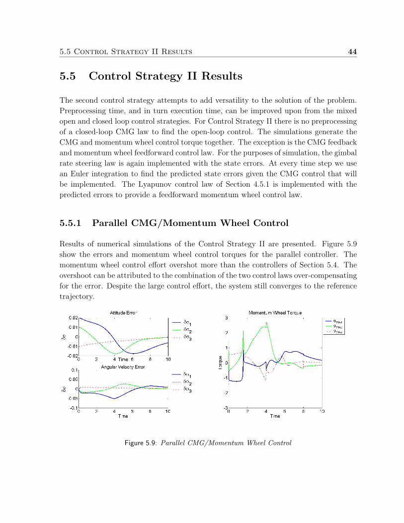
5.5 Control Strategy II Results 44
5.5 Control Strategy II Results
The second control strategy attempts to add versatility to the solution of the problem.
Preprocessing time, and in turn execution time, can be improved upon from the mixed
open and closed loop control strategies. For Control Strategy II there is no preprocessing
of a closed-loop CMG law to find the open-loop control. The simulations generate the
CMG and momentum wheel control torque together. The exception is the CMG feedback
and momentum wheel feedforward control law. For the purposes of simulation, the gimbal
rate steering law is again implemented with the state errors. At every time step we use
an Euler integration to find the predicted state errors given the CMG control that will
be implemented. The Lyapunov control law of Section 4.5.1 is implemented with the
predicted errors to provide a feedforward momentum wheel control law.
5.5.1 Parallel CMG/Momentum Wheel Control
Results of numerical simulations of the Control Strategy II are presented. Figure 5.9
show the errors and momentum wheel control torques for the parallel controller. The
momentum wheel control effort overshot more than the controllers of Section 5.4. The
overshoot can be attributed to the combination of the two control laws over-compensating
for the error. Despite the large control effort, the system still converges to the reference
trajectory.
Figure 5.9: Parallel CMG/Momentum Wheel Control
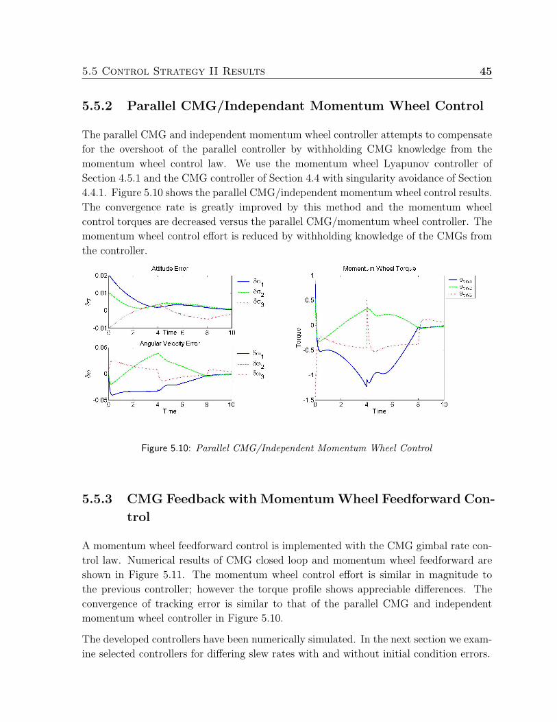
5.5 Control Strategy II Results 45
5.5.2 Parallel CMG/Independant Momentum Wheel Control
The parallel CMG and independent momentum wheel controller attempts to compensate
for the overshoot of the parallel controller by withholding CMG knowledge from the
momentum wheel control law. We use the momentum wheel Lyapunov controller of
Section 4.5.1 and the CMG controller of Section 4.4 with singularity avoidance of Section
4.4.1. Figure 5.10 shows the parallel CMG/independent momentum wheel control results.
The convergence rate is greatly improved by this method and the momentum wheel
control torques are decreased versus the parallel CMG/momentum wheel controller. The
momentum wheel control effort is reduced by withholding knowledge of the CMGs from
the controller.
Figure 5.10: Parallel CMG/Independent Momentum Wheel Control
5.5.3 CMG Feedback with Momentum Wheel Feedforward Con-
trol
A momentum wheel feedforward control is implemented with the CMG gimbal rate con-
trol law. Numerical results of CMG closed loop and momentum wheel feedforward are
shown in Figure 5.11. The momentum wheel control effort is similar in magnitude to
the previous controller; however the torque profile shows appreciable differences. The
convergence of tracking error is similar to that of the parallel CMG and independent
momentum wheel controller in Figure 5.10.
The developed controllers have been numerically simulated. In the next section we exam-
ine selected controllers for differing slew rates with and without initial condition errors.
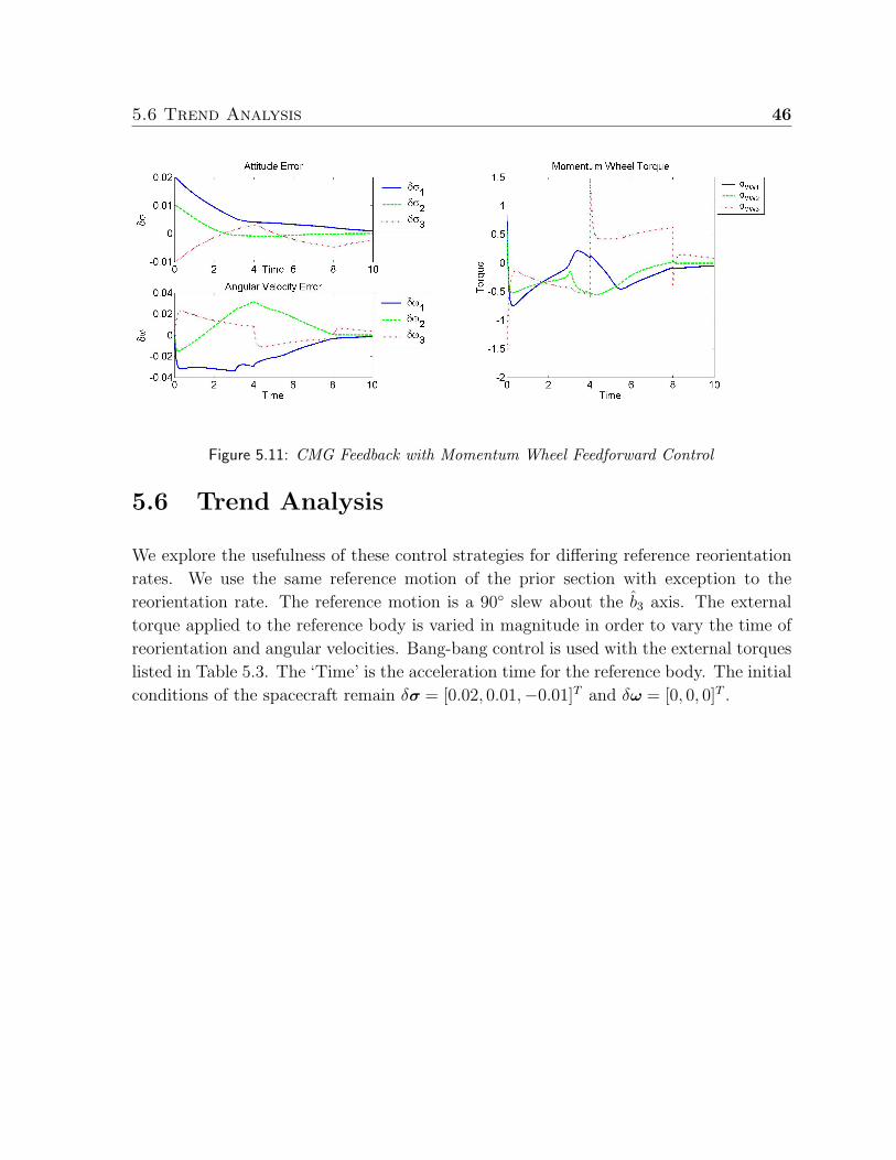
5.6 Trend Analysis 46
Figure 5.11: CMG Feedback with Momentum Wheel Feedforward Control
5.6 Trend Analysis
We explore the usefulness of these control strategies for differing reference reorientation
rates. We use the same reference motion of the prior section with exception to the
reorientation rate. The reference motion is a 90 slew about the b3 axis. The external
torque applied to the reference body is varied in magnitude in order to vary the time of
reorientation and angular velocities. Bang-bang control is used with the external torques
listed in Table 5.3. The ‘Time’ is the acceleration time for the reference body. The initial
conditions of the spacecraft remain δσ = [0.02, 0.01,−0.01]T and δω = [0, 0, 0]T .
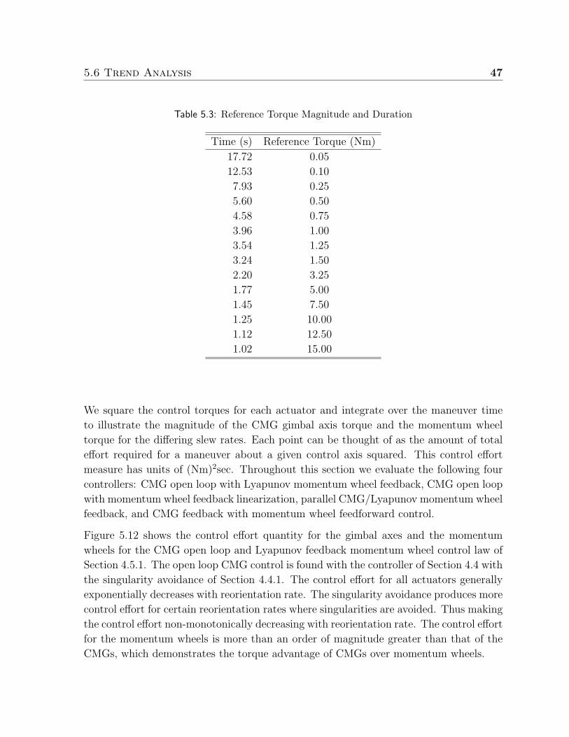
5.6 Trend Analysis 47
Table 5.3: Reference Torque Magnitude and Duration
Time (s) Reference Torque (Nm)
17.72 0.05
12.53 0.10
7.93 0.25
5.60 0.50
4.58 0.75
3.96 1.00
3.54 1.25
3.24 1.50
2.20 3.25
1.77 5.00
1.45 7.50
1.25 10.00
1.12 12.50
1.02 15.00
We square the control torques for each actuator and integrate over the maneuver time
to illustrate the magnitude of the CMG gimbal axis torque and the momentum wheel
torque for the differing slew rates. Each point can be thought of as the amount of total
effort required for a maneuver about a given control axis squared. This control effort
measure has units of (Nm)2sec. Throughout this section we evaluate the following four
controllers: CMG open loop with Lyapunov momentum wheel feedback, CMG open loop
with momentum wheel feedback linearization, parallel CMG/Lyapunov momentum wheel
feedback, and CMG feedback with momentum wheel feedforward control.
Figure 5.12 shows the control effort quantity for the gimbal axes and the momentum
wheels for the CMG open loop and Lyapunov feedback momentum wheel control law of
Section 4.5.1. The open loop CMG control is found with the controller of Section 4.4 with
the singularity avoidance of Section 4.4.1. The control effort for all actuators generally
exponentially decreases with reorientation rate. The singularity avoidance produces more
control effort for certain reorientation rates where singularities are avoided. Thus making
the control effort non-monotonically decreasing with reorientation rate. The control effort
for the momentum wheels is more than an order of magnitude greater than that of the
CMGs, which demonstrates the torque advantage of CMGs over momentum wheels.
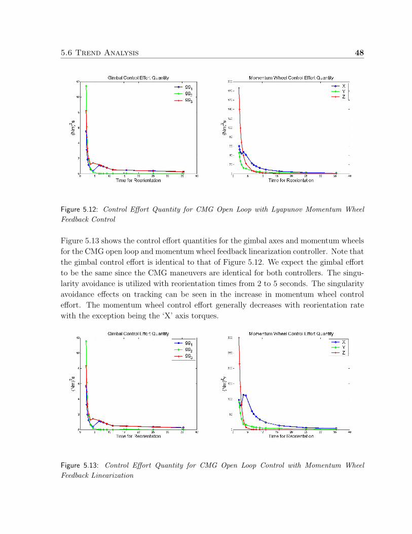
5.6 Trend Analysis 48
Figure 5.12: Control Effort Quantity for CMG Open Loop with Lyapunov Momentum WheelFeedback Control
Figure 5.13 shows the control effort quantities for the gimbal axes and momentum wheels
for the CMG open loop and momentum wheel feedback linearization controller. Note that
the gimbal control effort is identical to that of Figure 5.12. We expect the gimbal effort
to be the same since the CMG maneuvers are identical for both controllers. The singu-
larity avoidance is utilized with reorientation times from 2 to 5 seconds. The singularity
avoidance effects on tracking can be seen in the increase in momentum wheel control
effort. The momentum wheel control effort generally decreases with reorientation rate
with the exception being the ‘X’ axis torques.
Figure 5.13: Control Effort Quantity for CMG Open Loop Control with Momentum WheelFeedback Linearization
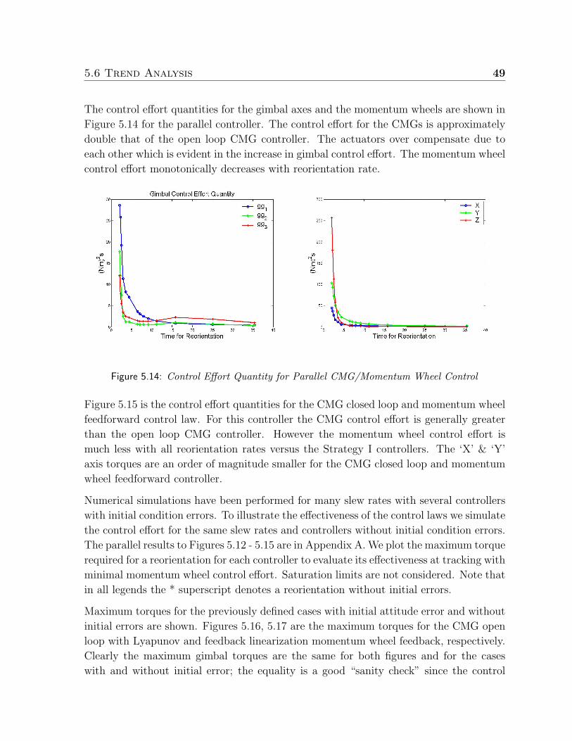
5.6 Trend Analysis 49
The control effort quantities for the gimbal axes and the momentum wheels are shown in
Figure 5.14 for the parallel controller. The control effort for the CMGs is approximately
double that of the open loop CMG controller. The actuators over compensate due to
each other which is evident in the increase in gimbal control effort. The momentum wheel
control effort monotonically decreases with reorientation rate.
Figure 5.14: Control Effort Quantity for Parallel CMG/Momentum Wheel Control
Figure 5.15 is the control effort quantities for the CMG closed loop and momentum wheel
feedforward control law. For this controller the CMG control effort is generally greater
than the open loop CMG controller. However the momentum wheel control effort is
much less with all reorientation rates versus the Strategy I controllers. The ‘X’ & ‘Y’
axis torques are an order of magnitude smaller for the CMG closed loop and momentum
wheel feedforward controller.
Numerical simulations have been performed for many slew rates with several controllers
with initial condition errors. To illustrate the effectiveness of the control laws we simulate
the control effort for the same slew rates and controllers without initial condition errors.
The parallel results to Figures 5.12 - 5.15 are in Appendix A. We plot the maximum torque
required for a reorientation for each controller to evaluate its effectiveness at tracking with
minimal momentum wheel control effort. Saturation limits are not considered. Note that
in all legends the * superscript denotes a reorientation without initial errors.
Maximum torques for the previously defined cases with initial attitude error and without
initial errors are shown. Figures 5.16, 5.17 are the maximum torques for the CMG open
loop with Lyapunov and feedback linearization momentum wheel feedback, respectively.
Clearly the maximum gimbal torques are the same for both figures and for the cases
with and without initial error; the equality is a good “sanity check” since the control
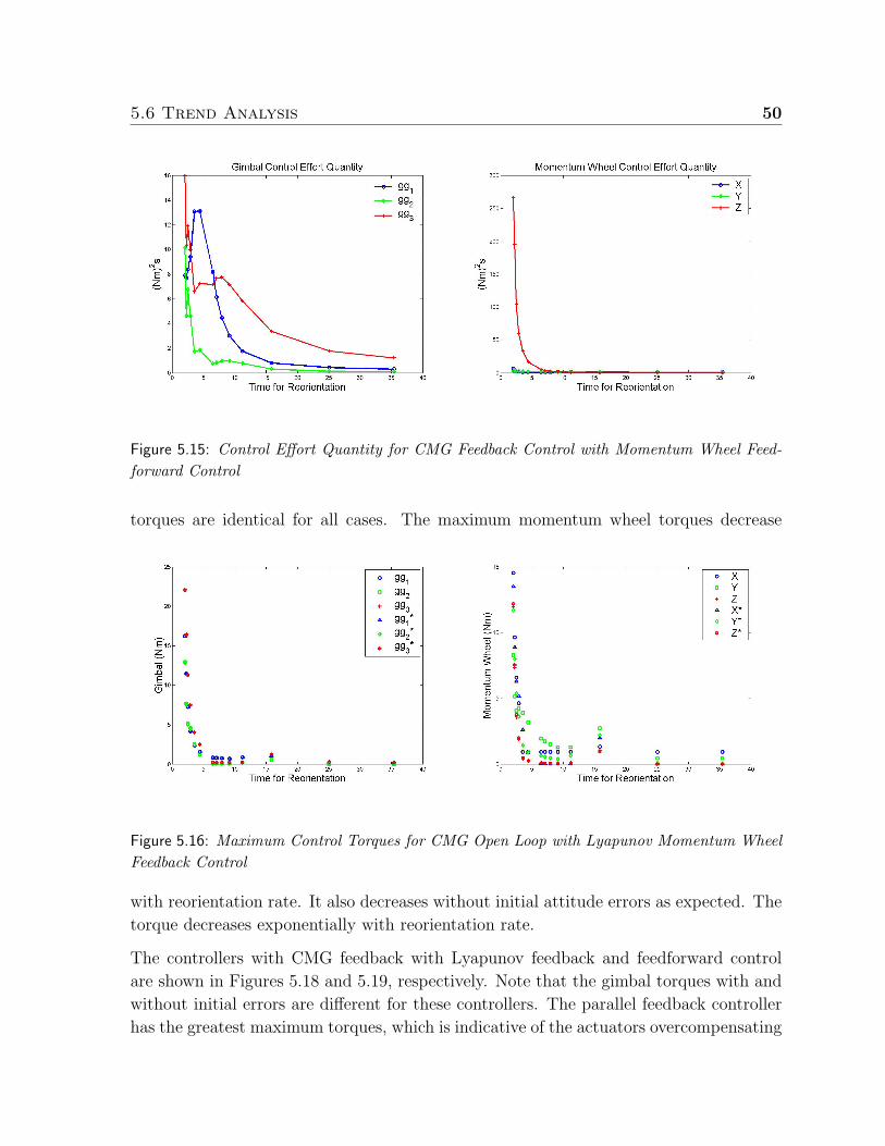
5.6 Trend Analysis 50
Figure 5.15: Control Effort Quantity for CMG Feedback Control with Momentum Wheel Feed-forward Control
torques are identical for all cases. The maximum momentum wheel torques decrease
Figure 5.16: Maximum Control Torques for CMG Open Loop with Lyapunov Momentum WheelFeedback Control
with reorientation rate. It also decreases without initial attitude errors as expected. The
torque decreases exponentially with reorientation rate.
The controllers with CMG feedback with Lyapunov feedback and feedforward control
are shown in Figures 5.18 and 5.19, respectively. Note that the gimbal torques with and
without initial errors are different for these controllers. The parallel feedback controller
has the greatest maximum torques, which is indicative of the actuators overcompensating
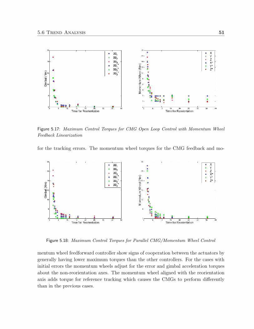
5.6 Trend Analysis 51
Figure 5.17: Maximum Control Torques for CMG Open Loop Control with Momentum WheelFeedback Linearization
for the tracking errors. The momentum wheel torques for the CMG feedback and mo-
Figure 5.18: Maximum Control Torques for Parallel CMG/Momentum Wheel Control
mentum wheel feedforward controller show signs of cooperation between the actuators by
generally having lower maximum torques than the other controllers. For the cases with
initial errors the momentum wheels adjust for the error and gimbal acceleration torques
about the non-reorientation axes. The momentum wheel aligned with the reorientation
axis adds torque for reference tracking which causes the CMGs to perform differently
than in the previous cases.
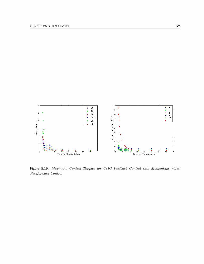
5.6 Trend Analysis 52
Figure 5.19: Maximum Control Torques for CMG Feedback Control with Momentum WheelFeedforward Control
53
Chapter 6
Virginia Tech Spacecraft Simulator
In this chapter we describe the spacecraft simulator at Virginia Tech, along with the
design of the single gimbal control moment gyro that is integrated on the simulator.
Sizing criteria for the CMG is discussed. The mixed actuator attitude control concept is
implemented with a single CMG and three momentum wheels. Results from simulator
testing are presented. The results verify the effectiveness of mixed actuator attitude
control. Sources of errors are presented.
6.1 Whorl-I
The ideal spherical air-bearing testbed would allow its payload unconstrained angular
motion in three axes. Actually providing this rotational freedom is difficult and in prac-
tice requires constraining payload volume. “Tabletop” style platforms, illustrated in
Figure 6.1, provide full freedom of spin in the yaw axis but pitch and roll motion are
typically constrained to angles of much less than ±90. The main structural deck of a
tabletop mounts to the flat face of a hemispherical bearing and components are attached
to this structure. Note that the yaw axis is defined to be nominally parallel to the gravity
vector.
The Virginia Tech Distributed Spacecraft Attitude Control System Simulator consists
of two air bearings from Space Electronics, Incorporated. Each can support a payload
of up to 300 lb. The tabletop platform provides full freedom in yaw and ±5 of tilt
in pitch and roll. As shown in Figure 6.1, the tabletop system, dubbed “Whorl-I”, is
complete. The primary structure is a 3 ft octagonal aluminum honeycomb plate. Large
components are mounted directly to threaded inserts installed in the honeycomb, and
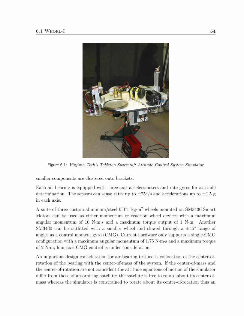
6.1 Whorl-I 54
Figure 6.1: Virginia Tech’s Tabletop Spacecraft Attitude Control System Simulator
smaller components are clustered onto brackets.
Each air bearing is equipped with three-axis accelerometers and rate gyros for attitude
determination. The sensors can sense rates up to ±75/s and accelerations up to ±1.5 g
in each axis.
A suite of three custom aluminum/steel 0.075 kg·m2 wheels mounted on SM3430 Smart
Motors can be used as either momentum or reaction wheel devices with a maximum
angular momentum of 10 N·m·s and a maximum torque output of 1 N·m. Another
SM3430 can be outfitted with a smaller wheel and slewed through a ±45 range of
angles as a control moment gyro (CMG). Current hardware only supports a single-CMG
configuration with a maximum angular momentum of 1.75 N·m·s and a maximum torque
of 2 N·m; four-axis CMG control is under consideration.
An important design consideration for air-bearing testbed is collocation of the center-of-
rotation of the bearing with the center-of-mass of the system. If the center-of-mass and
the center-of-rotation are not coincident the attitude equations of motion of the simulator
differ from those of an orbiting satellite: the satellite is free to rotate about its center-of-
mass whereas the simulator is constrained to rotate about its center-of-rotation thus an
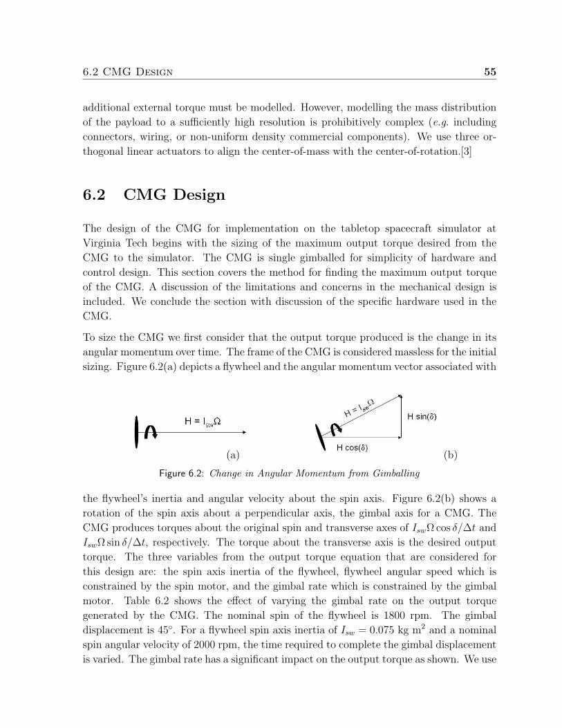
6.2 CMG Design 55
additional external torque must be modelled. However, modelling the mass distribution
of the payload to a sufficiently high resolution is prohibitively complex (e.g. including
connectors, wiring, or non-uniform density commercial components). We use three or-
thogonal linear actuators to align the center-of-mass with the center-of-rotation.[3]
6.2 CMG Design
The design of the CMG for implementation on the tabletop spacecraft simulator at
Virginia Tech begins with the sizing of the maximum output torque desired from the
CMG to the simulator. The CMG is single gimballed for simplicity of hardware and
control design. This section covers the method for finding the maximum output torque
of the CMG. A discussion of the limitations and concerns in the mechanical design is
included. We conclude the section with discussion of the specific hardware used in the
CMG.
To size the CMG we first consider that the output torque produced is the change in its
angular momentum over time. The frame of the CMG is considered massless for the initial
sizing. Figure 6.2(a) depicts a flywheel and the angular momentum vector associated with
(a) (b)
Figure 6.2: Change in Angular Momentum from Gimballing
the flywheel’s inertia and angular velocity about the spin axis. Figure 6.2(b) shows a
rotation of the spin axis about a perpendicular axis, the gimbal axis for a CMG. The
CMG produces torques about the original spin and transverse axes of IswΩ cos δ/∆t and
IswΩ sin δ/∆t, respectively. The torque about the transverse axis is the desired output
torque. The three variables from the output torque equation that are considered for
this design are: the spin axis inertia of the flywheel, flywheel angular speed which is
constrained by the spin motor, and the gimbal rate which is constrained by the gimbal
motor. Table 6.2 shows the effect of varying the gimbal rate on the output torque
generated by the CMG. The nominal spin of the flywheel is 1800 rpm. The gimbal
displacement is 45. For a flywheel spin axis inertia of Isw = 0.075 kg m2 and a nominal
spin angular velocity of 2000 rpm, the time required to complete the gimbal displacement
is varied. The gimbal rate has a significant impact on the output torque as shown. We use
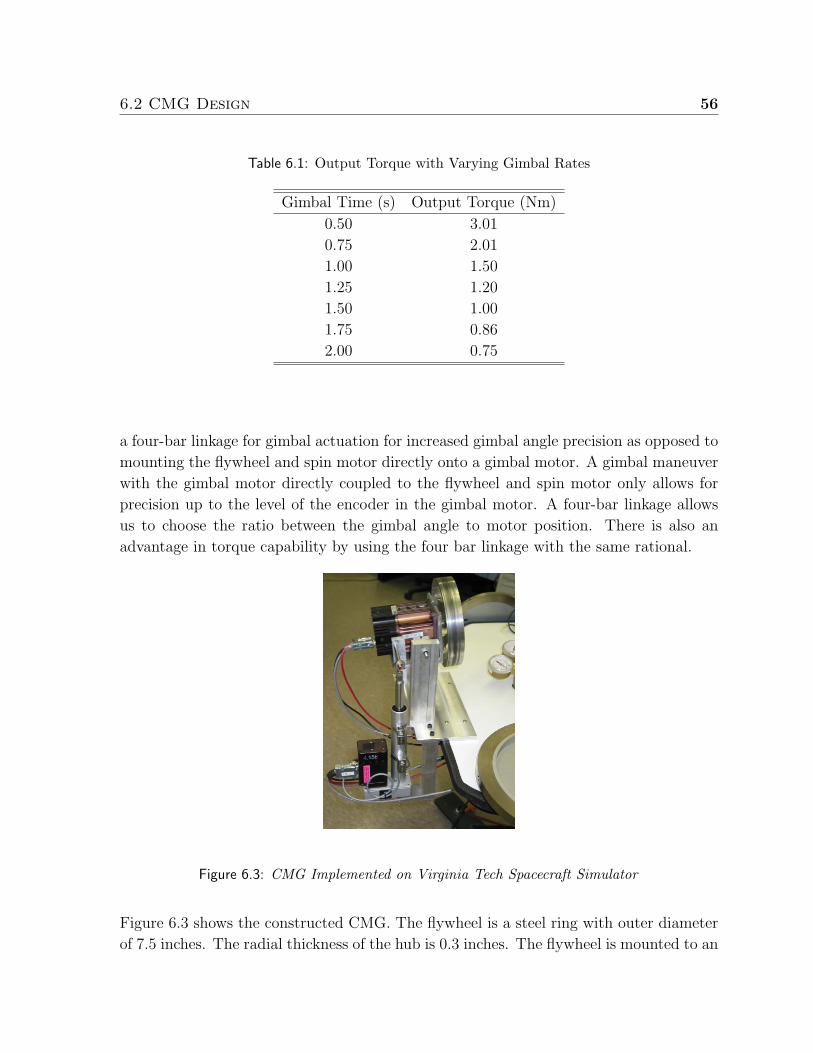
6.2 CMG Design 56
Table 6.1: Output Torque with Varying Gimbal Rates
Gimbal Time (s) Output Torque (Nm)
0.50 3.01
0.75 2.01
1.00 1.50
1.25 1.20
1.50 1.00
1.75 0.86
2.00 0.75
a four-bar linkage for gimbal actuation for increased gimbal angle precision as opposed to
mounting the flywheel and spin motor directly onto a gimbal motor. A gimbal maneuver
with the gimbal motor directly coupled to the flywheel and spin motor only allows for
precision up to the level of the encoder in the gimbal motor. A four-bar linkage allows
us to choose the ratio between the gimbal angle to motor position. There is also an
advantage in torque capability by using the four bar linkage with the same rational.
Figure 6.3: CMG Implemented on Virginia Tech Spacecraft Simulator
Figure 6.3 shows the constructed CMG. The flywheel is a steel ring with outer diameter
of 7.5 inches. The radial thickness of the hub is 0.3 inches. The flywheel is mounted to an
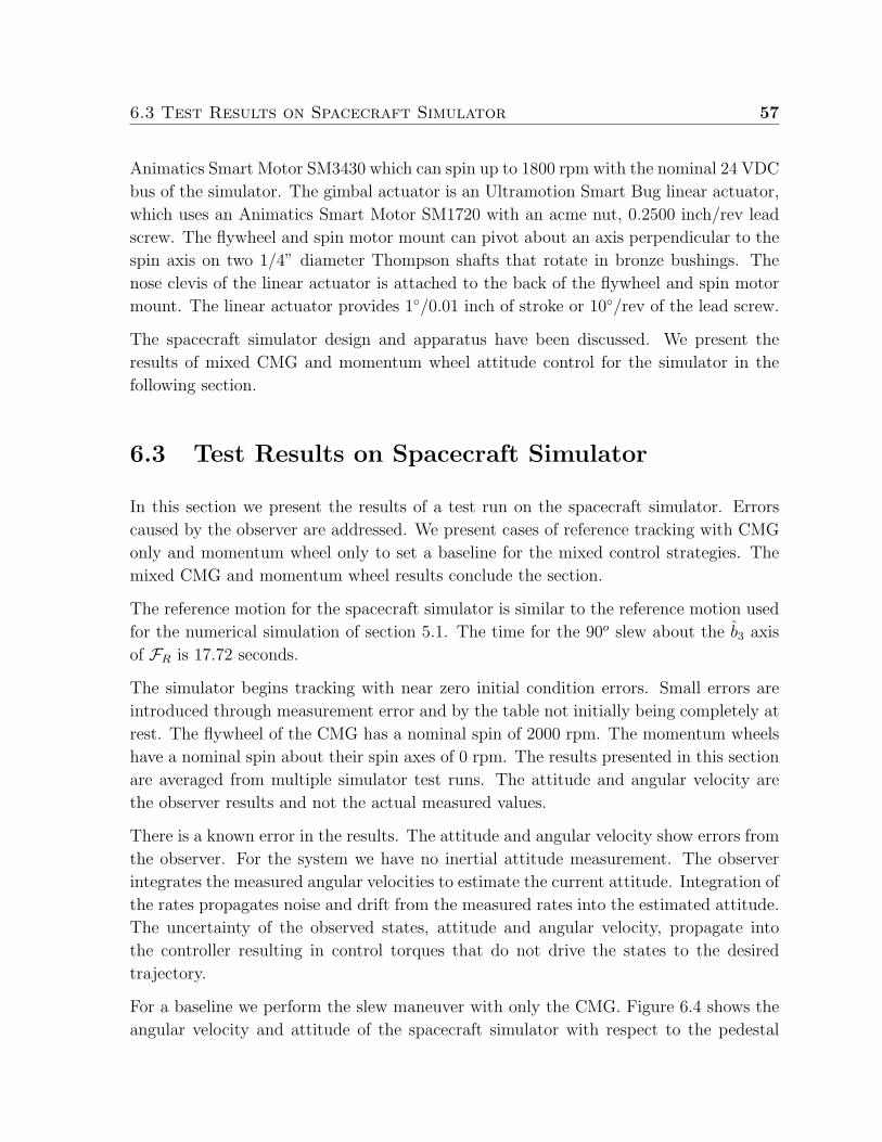
6.3 Test Results on Spacecraft Simulator 57
Animatics Smart Motor SM3430 which can spin up to 1800 rpm with the nominal 24 VDC
bus of the simulator. The gimbal actuator is an Ultramotion Smart Bug linear actuator,
which uses an Animatics Smart Motor SM1720 with an acme nut, 0.2500 inch/rev lead
screw. The flywheel and spin motor mount can pivot about an axis perpendicular to the
spin axis on two 1/4” diameter Thompson shafts that rotate in bronze bushings. The
nose clevis of the linear actuator is attached to the back of the flywheel and spin motor
mount. The linear actuator provides 1/0.01 inch of stroke or 10/rev of the lead screw.
The spacecraft simulator design and apparatus have been discussed. We present the
results of mixed CMG and momentum wheel attitude control for the simulator in the
following section.
6.3 Test Results on Spacecraft Simulator
In this section we present the results of a test run on the spacecraft simulator. Errors
caused by the observer are addressed. We present cases of reference tracking with CMG
only and momentum wheel only to set a baseline for the mixed control strategies. The
mixed CMG and momentum wheel results conclude the section.
The reference motion for the spacecraft simulator is similar to the reference motion used
for the numerical simulation of section 5.1. The time for the 90o slew about the b3 axis
of FR is 17.72 seconds.
The simulator begins tracking with near zero initial condition errors. Small errors are
introduced through measurement error and by the table not initially being completely at
rest. The flywheel of the CMG has a nominal spin of 2000 rpm. The momentum wheels
have a nominal spin about their spin axes of 0 rpm. The results presented in this section
are averaged from multiple simulator test runs. The attitude and angular velocity are
the observer results and not the actual measured values.
There is a known error in the results. The attitude and angular velocity show errors from
the observer. For the system we have no inertial attitude measurement. The observer
integrates the measured angular velocities to estimate the current attitude. Integration of
the rates propagates noise and drift from the measured rates into the estimated attitude.
The uncertainty of the observed states, attitude and angular velocity, propagate into
the controller resulting in control torques that do not drive the states to the desired
trajectory.
For a baseline we perform the slew maneuver with only the CMG. Figure 6.4 shows the
angular velocity and attitude of the spacecraft simulator with respect to the pedestal
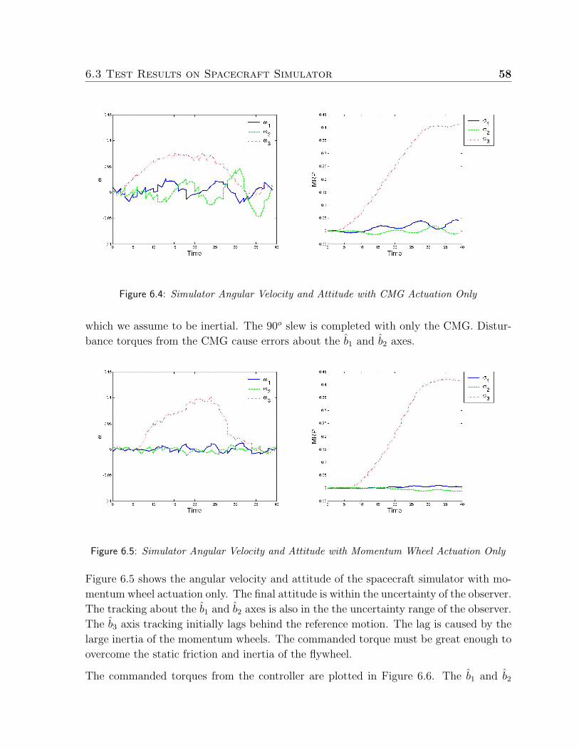
6.3 Test Results on Spacecraft Simulator 58
Figure 6.4: Simulator Angular Velocity and Attitude with CMG Actuation Only
which we assume to be inertial. The 90o slew is completed with only the CMG. Distur-
bance torques from the CMG cause errors about the b1 and b2 axes.
Figure 6.5: Simulator Angular Velocity and Attitude with Momentum Wheel Actuation Only
Figure 6.5 shows the angular velocity and attitude of the spacecraft simulator with mo-
mentum wheel actuation only. The final attitude is within the uncertainty of the observer.
The tracking about the b1 and b2 axes is also in the the uncertainty range of the observer.
The b3 axis tracking initially lags behind the reference motion. The lag is caused by the
large inertia of the momentum wheels. The commanded torque must be great enough to
overcome the static friction and inertia of the flywheel.
The commanded torques from the controller are plotted in Figure 6.6. The b1 and b2
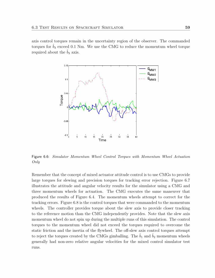
6.3 Test Results on Spacecraft Simulator 59
axis control torques remain in the uncertainty region of the observer. The commanded
torques for b3 exceed 0.1 Nm. We use the CMG to reduce the momentum wheel torque
required about the b3 axis.
Figure 6.6: Simulator Momentum Wheel Control Torques with Momentum Wheel ActuationOnly
Remember that the concept of mixed actuator attitude control is to use CMGs to provide
large torques for slewing and precision torques for tracking error rejection. Figure 6.7
illustrates the attitude and angular velocity results for the simulator using a CMG and
three momentum wheels for actuation. The CMG executes the same maneuver that
produced the results of Figure 6.4. The momentum wheels attempt to correct for the
tracking errors. Figure 6.8 is the control torques that were commanded to the momentum
wheels. The controller provides torque about the slew axis to provide closer tracking
to the reference motion than the CMG independently provides. Note that the slew axis
momentum wheel do not spin up during the multiple runs of this simulation. The control
torques to the momentum wheel did not exceed the torques required to overcome the
static friction and the inertia of the flywheel. The off-slew axis control torques attempt
to reject the torques created by the CMGs gimballing. The b1 and b2 momentum wheels
generally had non-zero relative angular velocities for the mixed control simulator test
runs.
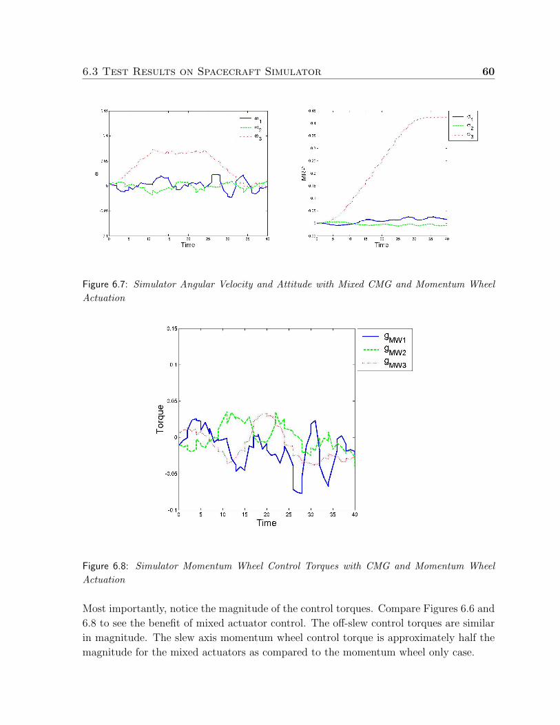
6.3 Test Results on Spacecraft Simulator 60
Figure 6.7: Simulator Angular Velocity and Attitude with Mixed CMG and Momentum WheelActuation
Figure 6.8: Simulator Momentum Wheel Control Torques with CMG and Momentum WheelActuation
Most importantly, notice the magnitude of the control torques. Compare Figures 6.6 and
6.8 to see the benefit of mixed actuator control. The off-slew control torques are similar
in magnitude. The slew axis momentum wheel control torque is approximately half the
magnitude for the mixed actuators as compared to the momentum wheel only case.
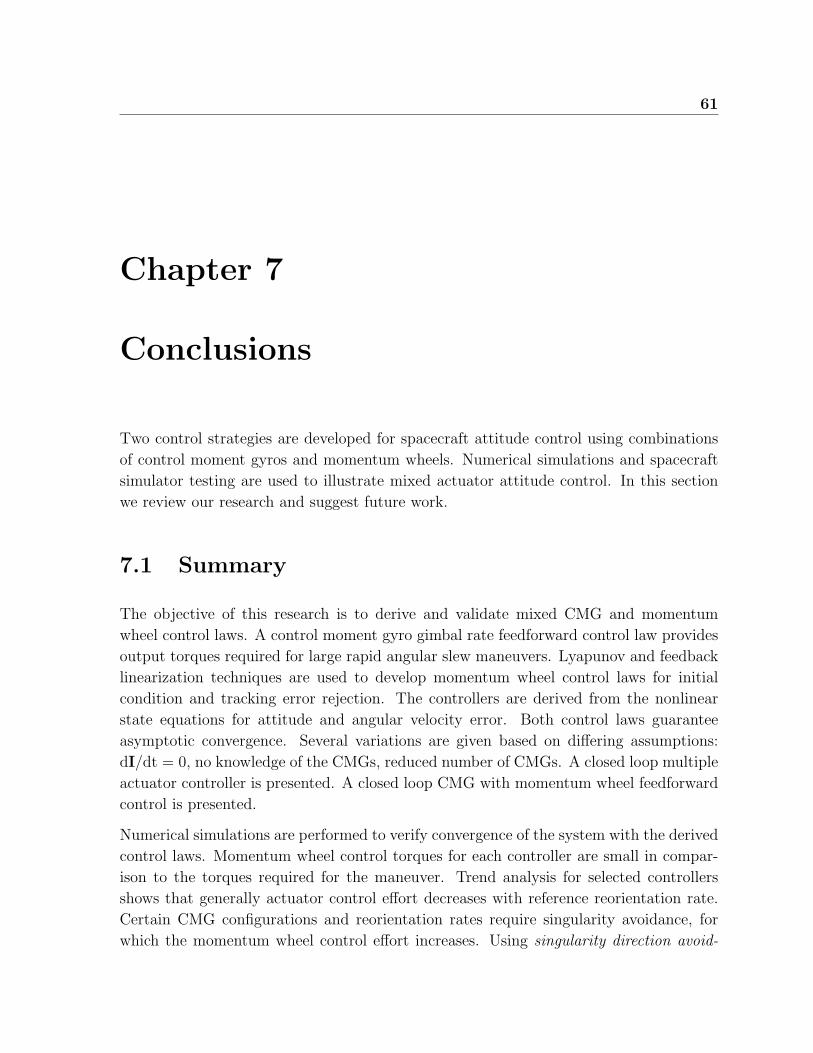
61
Chapter 7
Conclusions
Two control strategies are developed for spacecraft attitude control using combinations
of control moment gyros and momentum wheels. Numerical simulations and spacecraft
simulator testing are used to illustrate mixed actuator attitude control. In this section
we review our research and suggest future work.
7.1 Summary
The objective of this research is to derive and validate mixed CMG and momentum
wheel control laws. A control moment gyro gimbal rate feedforward control law provides
output torques required for large rapid angular slew maneuvers. Lyapunov and feedback
linearization techniques are used to develop momentum wheel control laws for initial
condition and tracking error rejection. The controllers are derived from the nonlinear
state equations for attitude and angular velocity error. Both control laws guarantee
asymptotic convergence. Several variations are given based on differing assumptions:
dI/dt = 0, no knowledge of the CMGs, reduced number of CMGs. A closed loop multiple
actuator controller is presented. A closed loop CMG with momentum wheel feedforward
control is presented.
Numerical simulations are performed to verify convergence of the system with the derived
control laws. Momentum wheel control torques for each controller are small in compar-
ison to the torques required for the maneuver. Trend analysis for selected controllers
shows that generally actuator control effort decreases with reference reorientation rate.
Certain CMG configurations and reorientation rates require singularity avoidance, for
which the momentum wheel control effort increases. Using singularity direction avoid-
7.2 Recommended Future Work 62
ance can reduce the tracking error and momentum wheel control effort that is caused by
avoiding CMG singular configurations.
Implementation of one CMG and three orthogonal momentum wheels on a spacecraft
simulator illustrated the mixed actuator attitude control concept. The spacecraft simu-
lator had tracking errors due to observer errors. Overall the controller showed promise.
7.2 Recommended Future Work
The focus of this research was to derive mixed CMG and momentum wheel attitude
controllers and prove that the derived controllers caused the system to converge to the
reference motion. The next step for the derived controllers is optimization of gain selec-
tion, and comparison between the controllers with optimal gains. For this purpose the
optimal gain solution would minimize control effort. Future work should include power
studies of mixed CMG and momentum wheel attitude control versus momentum wheel
control to verify the advantage of the mixed actuator attitude control concept.
The configuration of one CMG with a momentum wheel cluster, both in closed loop
control, seems promising. The problem is under-constrained, which will require optimal
control techniques to solve. Adapting previous null-motion solutions, such as in Ref. [16],
to one CMG with momentum wheels might provide a means of optimally configuring the
CMG.
63
Bibliography
[1] B. Wie, Q. Liu, and F. Bauer, “Classical and robust H∞ control redesign for the
Hubble Space Telescope,” Journal of Guidance, Control, and Dynamics, vol. 16,
no. 6, pp. 1069–1077, 1993.
[2] C. D. Hall, P. Tsiotras, and H. Shen, “Tracking rigid body motion using thrusters
and momentum wheels,” The Journal of the Astronautical Sciences, vol. 50, no. 3,
2002.
[3] J. L. Schwartz, M. A. Peck, and C. D. Hall, “Historical review of air-bearing space-
craft simulators,” Journal of Guidance, Control, and Dynamics, vol. 26, no. 4,
pp. 513–522, 2003.
[4] K. A. Ford, Reorientations of Flexible Spacecraft Using Momentum Exchange De-
vices. PhD thesis, Air Force Institute of Technology, Dayton, OH, 1997.
[5] P. Tsiotras, “Stabilization and optimality results for the attitude control problem,”
Journal of Guidance, Control, and Dynamics, vol. 19, pp. 772–779, July 1996.
[6] P. C. Hughes, Spacecraft Attitude Dynamics. New York, New York: John Wiley and
Sons, 1986.
[7] C. D. Hall, “Spinup dynamics of gyrostats,” Journal of Guidance, Control, and
Dynamics, vol. 18, no. 5, pp. 1177–1183, 1995.
[8] C. D. Hall, “High speed flywheels for integrated energy storage and attitude control,”
in Proceedings of the American Control Conference, (Albuquerque, NM), pp. 1894–
1898, June 1997.
[9] C. D. Hall, P. Tsiotras, and H. Shen, “Satellite attitude control and power track-
ing with momentum/energy wheels,” Journal of Guidance, Control, and Dynamics,
vol. 24, no. 1, pp. 23–34, 2001.
BIBLIOGRAPHY 64
[10] B. T. Costic, Energy Management and Attitude Control Strategies using Flywheels.
PhD thesis, Clemson University, 2001.
[11] J. L. Junkins, M. R. Akella, and R. D. Robinett, “Nonlinear adaptive control of
spacecraft maneuvers,” in Proceedings of the AIAA Guidance, Navigation, and Con-
trol Conference, no. 97-3480, (New Orleans, LA), August 1997.
[12] H. S. Oh and S. R. Vadali, “Feedback control and steering laws for spacecraft using
single gimbal control moment gyros,” Journal of the Astronautical Sciences, vol. 38,
pp. 183–203, April 1991.
[13] S. R. Vadali, H. S. Oh, and S. R. Walker, “Preferred gimbal angles for single gimbal
control moment gyros,” Journal of Guidance, Control, and Dynamics, vol. 13, no. 6,
pp. 1090–1095, 1990.
[14] S. R. Vadali and S. Krishnan, “Suboptimal command generation for control moment
gyroscopes and feedback control of spacecraft,” Journal of Guidance, Control, and
Dynamics, vol. 18, no. 6, pp. 1350–1354, 1995.
[15] B. R. Hoelscher and S. R. Vadali, “Optimal open-loop and feedback control using
single gimbal control moment gyroscopes,” The Journal of the Astronautical Sci-
ences, vol. 42, pp. 189–206, April 1994.
[16] K. A. Ford and C. D. Hall, “Singular direction avoidance steering for control-moment
gyros,” Journal of Guidance, Control, and Dynamics, vol. 23, pp. 648–656, July
2000.
[17] M. R. Rokui and S. Kalaycioglu, “Control moment gyro (CMG) based spacecraft
attitude control using feedback linearization control technique,” Advances in the
Astronautical Sciences, vol. 97, no. 1, pp. 983–997, 1997.
[18] H. Schaub, S. R. Vadali, and J. L. Junkins, “Feedback control law for variable speed
control moment gyros,” Journal of the Astronautical Sciences, vol. 46, pp. 307–328,
July 1998.
[19] G. Avanzini and G. de Matteis, “A local optimization technique for attitude mo-
tion tracking using control moment gyroscopes,” The Journal of the Astronautical
Sciences, vol. 50, no. 2, pp. 213–229, 2002.
[20] C. J. Heiberg, D. Bailey, and B. Wie, “Precision pointing control of agile spacecraft
using single gimbal control moment gyroscopes,” in Proceedings of the AIAA Guid-
ance, Navigation, and Control Conference, no. 97-3757, (New Orleans, LA), August
1997.
BIBLIOGRAPHY 65
[21] B. Wie, C. J. Heiberg, and D. Bailey, “Rapid multi-target acquisition and pointing
control of agile spacecraft,” in Proceedings of the AIAA Guidance, Navigation, and
Control Conference and Exhibit, no. 00-4546, (Denver, CO), August 2000.
[22] S. N. Singh and T. C. Bossart, “Exact feedback linearization and control of space
station using CMG,” IEEE Transactions on Automatic Control, vol. 38, pp. 184–187,
January 1993.
[23] M. R. Long, “Spacecraft attitude tracking control,” Master’s thesis, Virginia Tech,
Blacksburg, VA, 1999.
[24] M. Casasco and G. Radice, “Autonomous slew maneuvering and attitude control us-
ing the potential function method,” in Proceedings of the AAS/AIAA Astrodynamics
Specialists Conference, no. 03-612, (Big Sky, MT), August 2003.
[25] X. Chen and W. H. Steyn, “Robust combined eigenaxis slew maneuver,” in Pro-
ceedings of the AIAA Guidance, Navigation, and Control Conference and Exhibit,
no. 99-4048, (Portland, OR), August 1999.
[26] C. M. Roithmayr, C. D. Karlgaard, R. R. Kumar, H. Seywald, and D. M. Bose,
“Dynamics and control of attitude, power, and momentum for a spacecraft using
flywheels and control moment gyroscopes,” Langley Technical Report, no. 212178,
2003.
[27] V. Lappas, W. Steyn, and C. Underwood, “Control moment gyro gimbal angle
compensation using magnetic control during external disturbances,” in Proceedings
of the AIAA Guidance, Navigation, and Control Conference and Exhibit, no. 01-
4339, (Montreal, Canada), August 2001.
[28] H. Schaub and J. L. Junkins, “CMG singularity avoidance using VSCMG null mo-
tion,” in AIAA/AAS Astrodynamics Specialist Conference and Exhibit, no. 98-4388,
(Boston, MA), August 1998.
[29] M. A. Peck, L. Miller, A. Cavender, M. Gonzalez, and T. Hintz, “An airbearing-
based testbed for momentum control systems and spacecraft line of sight,” in Pro-
ceedings of the 13th AAS/AIAA Space Flight Mechanics Meeting, no. 03-127, (Ponce,
Puerto Rico), February 2003.
[30] J. J. Kalley and H. L. Mork, “Development and air bearing test of a double gimballed
momentum wheel attitude control system,” in AIAA Communications Satellite Sys-
tems Conference, (Las Angels, CA), April 1974.
BIBLIOGRAPHY 66
[31] A. Ramos, “Air bearing platform testing of a double-gimballed momentum wheel
attitude control system,” COMSAT Technical Review, vol. 5, pp. 53–72, 1975.
[32] H. Kurokawa, “Constrained steering law of pyramid type CMGs and ground tests,”
in Proceedings of the AIAA Guidance, Navigation, and Control Conference, no. 96-
3790, (San Diego, CA), July 1996.
[33] J. E. Colebank, R. D. Jones, G. R. Nagy, R. D. Pollak, and D. R. Mannebach,
“Simsat: A satellite simulator and experimental test bed for Air Force research,”
in Proceedings of the AIAA Space Technology Conference and Exposition, (Albu-
querque, NM), September 1999.
[34] S. Cho and N. H. McClamroch, “Feedback control of triaxial attitude control testbed
actuated by two proof mass devices,” in Proceedings of the 41th IEEE Conference
of Decision and Control, (Las Vegas, NV), December 2002.
[35] B. Kim, E. Velenis, P. Kriengsiri, and P. Tsiotras, “A spacecraft simulator for re-
search and education,” in Proceedings of the AIAA Guidance, Dynamics and Control
Conference, no. 01-367, (Reno, NV), pp. 897–914, 2001.
[36] M. D. Shuster, “A survey of attitude representations,” The Journal of the Astro-
nautical Sciences, vol. 41, no. 4, pp. 439–518, 1993.
[37] H. K. Khalil, Nonlinear Systems. New York, New York: Macmillian, 1992.
[38] S. Sastry, Nonlinear Systems. New York, New York: Springer, 1999.
[39] J. J. Slotine and W. Li, Applied Nonlinear Control. Englewood Cliffs, New Jersy:
Prentice Hall, 1991.
[40] H. Schaub and J. L. Junkins, “Matlab toolbox for rigid body kinematics,” Advances
in the Astronautical Sciences, vol. 102, pp. 549–560, 1999.
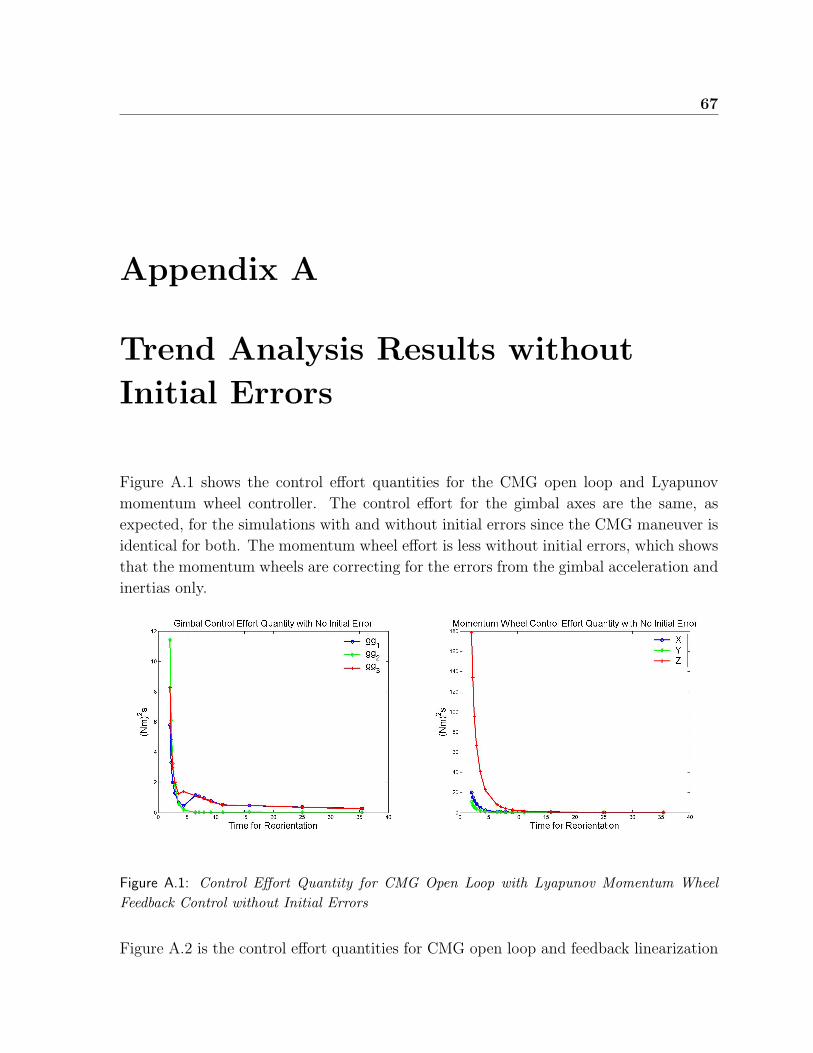
67
Appendix A
Trend Analysis Results without
Initial Errors
Figure A.1 shows the control effort quantities for the CMG open loop and Lyapunov
momentum wheel controller. The control effort for the gimbal axes are the same, as
expected, for the simulations with and without initial errors since the CMG maneuver is
identical for both. The momentum wheel effort is less without initial errors, which shows
that the momentum wheels are correcting for the errors from the gimbal acceleration and
inertias only.
Figure A.1: Control Effort Quantity for CMG Open Loop with Lyapunov Momentum WheelFeedback Control without Initial Errors
Figure A.2 is the control effort quantities for CMG open loop and feedback linearization
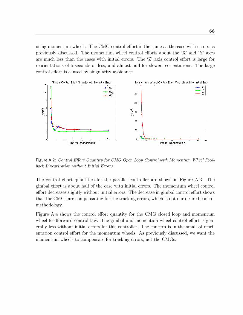
68
using momentum wheels. The CMG control effort is the same as the case with errors as
previously discussed. The momentum wheel control efforts about the ‘X’ and ‘Y’ axes
are much less than the cases with initial errors. The ‘Z’ axis control effort is large for
reorientations of 5 seconds or less, and almost null for slower reorientations. The large
control effort is caused by singularity avoidance.
Figure A.2: Control Effort Quantity for CMG Open Loop Control with Momentum Wheel Feed-back Linearization without Initial Errors
The control effort quantities for the parallel controller are shown in Figure A.3. The
gimbal effort is about half of the case with initial errors. The momentum wheel control
effort decreases slightly without initial errors. The decrease in gimbal control effort shows
that the CMGs are compensating for the tracking errors, which is not our desired control
methodology.
Figure A.4 shows the control effort quantity for the CMG closed loop and momentum
wheel feedforward control law. The gimbal and momentum wheel control effort is gen-
erally less without initial errors for this controller. The concern is in the small of reori-
entation control effort for the momentum wheels. As previously discussed, we want the
momentum wheels to compensate for tracking errors, not the CMGs.
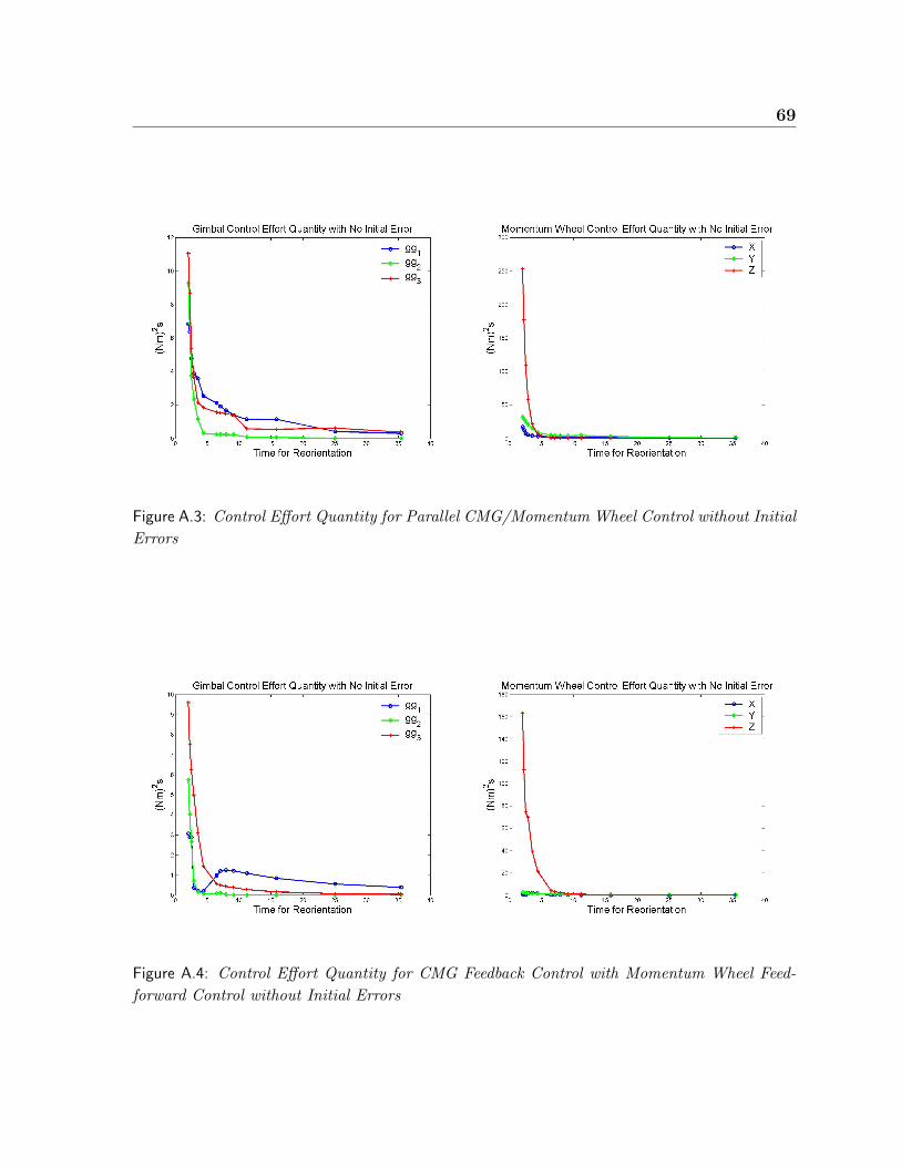
69
Figure A.3: Control Effort Quantity for Parallel CMG/Momentum Wheel Control without InitialErrors
Figure A.4: Control Effort Quantity for CMG Feedback Control with Momentum Wheel Feed-forward Control without Initial Errors
70
Vita
Claude Eugene Skelton II was born into an United States Air Force family in Okinawa,
Japan. He graduated from Westlake High School in 1996. In the fall of the same year
he began college at Virginia Polytechnic Institute & State University (Virginia Tech).
He funded his undergraduate career through constant employment, most semesters with
multiple jobs. Eugene graduated in May 2000 with a Bachelor of Science in Mechanical
Engineering. Eugene was employed in June 2000 by the AVX Corporation in Myrtle
Beach, SC as a Mechanical Engineer providing automated machine design.
With hopes of pursuing a more challenging career, he went back for graduate school
Virginia Tech in Aerospace Engineering. After a short time he found the Space Sys-
tems Simulation Laboratory where he conducted his research on mixed actuator attitude
control.
In September 2003 Eugene started with CENTRA Technology, Inc. in Arlington, Vir-
ginia. He currently is an Aerospace Engineering Systems Engineering and Technical
Analysis (SETA) support contractor for Defense Advanced Research Projects Agency
(DARPA) program managers.