Embed Size (px)
Citation preview

14.581 MIT PhD International Trade – Lecture 11: Heterogeneous Firms and Trade (Theory
part I) –
Dave Donaldson
Spring 2011

1
2
1
2
Today’s Plan
Introduction to “New New” Trade Theory
Melitz (Ecta, 2003)
Closed economy.
Open economy with variable and fixed trade costs.

’
1
2
3
4
5
“New New” Trade Theory What s wrong with previous theories?
• The 1990s saw a boom in the availability of micro-level data covering firms/plants. This changed many fields and Trade was no exception.
• Problem: both neoclassical and new trade theory are at odds with (or cannot account for) many micro-level facts that became apparent in this data:
Within a given industry, there is firm-level heterogeneity (eg inproductivity levels).
Fixed costs matter in export related decisions.
Within a given industry, more productive firms are more likely to export.
Trade liberalization leads to intra-industry reallocation across firms.
These reallocations are correlated with productivity and export status (so industry productivity can rise purely due to trade-driven selection).

1
2
“New New” Trade Theory What does Melitz (2003) do about it?
• Melitz (2003) develops a model featuring facts 1 and 2 that can explain facts 3, 4, and 5.
• This has been an extremely infiuential paper and modeling approach in both Trade and other fields (2,900 cites on Google Scholar!)
• Two building blocks:
Krugman (AER, 1980): CES, IRS technology, monopolistic competition.
Hopenhayn (Ecta, 1992): equilibrium model of entry and exit.
• From a normative point of view, Melitz (2003) may also provide new source of gains from trade if trade induces reallocation of labor from least to most productive firms (more on that later).
1
2
1
2
Today’s Plan
Introduction to “New New” Trade Theory
Melitz (Ecta, 2003)
Closed economy.
Open economy with variable and fixed trade costs.

� �
Melitz (2003) Demand
• Like in Krugman (1980), representative agent has CES preferences: �� � σ
σU = q (ω) σ−1 dω
σ−1
ω∈Ω
where σ > 1 is the elasticity of substitution (and let ρ ≡ (σ − 1)/σ). • Consumption and expenditures for each variety ω are given by
q (ω) = Qp (ω) −σ
(1)P
r (ω) = R
� p (ω)
�1−σ
(2)P
where: �� � 1 � P ≡
ω∈Ω p (ω)1−σ dω
1−σ
, R ≡ ω∈Ω
r (ω) , and Q ≡ R/P

Melitz (2003) Production
• Like in Krugman (1980), labor is the only factor of production • L ≡ total endowment, w = 1 ≡ wage
• Like in Krugman (1980), there are IRTS in production
l = f + q/ϕ (3)
• Like in Krugman (1980), monopolistic competition implies
1 p (ϕ) = (4)
ρϕ
• CES preferences with monopoly pricing, (2) and (4), imply
r (ϕ) = R (Pρϕ)σ−1 (5)
• These two assumptions, (3) and (4), further imply
π (ϕ) ≡ r (ϕ) − l (ϕ) = r (ϕ) − f
σ

1
2
3
� �
Melitz (2003) Production
Comments:• In (extremely common) cases where statistical agencies can’t collect firm-specific price defiators, higher productivity ϕ in the model also implies higher measured productivity:
lr ((
ϕ
ϕ
)
) = 1 ρ 1 −
l (f ϕ)
More productive firms produce more and earn higher revenues
q (ϕ1) �
ϕ1 �σ r (ϕ1)
� ϕ1 �σ−1
= and = q (ϕ2) ϕ2 r (ϕ2) ϕ2
ϕ can also be interpreted in terms of quality. This is isomorphic to a change in units of account, which would affect prices, but nothing else.

Melitz (2003) Aggregation
• By definition, the CES price index is given by: �� � 1
P = p (ω)1−σ dω 1−σ
ω∈Ω
• Since all firms with productivity ϕ charge the same price p (ϕ), we can rearrange the CES price index as: �� � 1
P =+∞ p (ϕ)1−σ Mµ (ϕ) d ϕ
1−σ
0
where:
• M ≡ mass of (surviving) firms in equilibrium.
• µ (ϕ) ≡ (conditional) pdf of firm-productivity levels in equilibrium.

1
2
Melitz (2003) Aggregation
• Combining the previous expression with monopoly pricing (4), we get
1 P = M 1−σ /ρ�ϕ
where �� +∞ � 1 �ϕ ≡
0 ϕσ−1 µ (ϕ) d ϕ
σ−1
• Conveniently, one can do the same for all aggregate variables
σ R = Mr (�ϕ) , Π = Mπ (ϕ�) , Q = M σ−1 q (�ϕ)
Comments:• These are the same aggregate variables we would get in a Krugman (1980) model with a mass M of identical firms with productivity �ϕ. But productivity �ϕ now is an endogenous variable which may respond to changes in trade cost, leading to aggregate productivity changes.

1
2
3
4
Melitz (2003) Entry and exit
• In order to determine how µ (ϕ) and �ϕ get determined in equilibrium, one needs to specify the entry and exit of firms.
• Timing is similar to Hopenhayn (1992):
There is a large pool of identical potential entrants deciding whether to become active or not.
Firms deciding to become active pay a fixed cost of entry fe > 0 and then get a productivity draw ϕ from a cdf G .
After observing their productivity draws, firms decide whether toremain active or not.
Firms deciding to remain active exit with a constant probability δ.

1
2
Melitz (2003) Aside: Pareto distributions
• In variations and extensions of Melitz (2003), most common assumption on the productivity distribution G (.) is Pareto: � �θϕ
G (ϕ) ≡ 1 − ϕ
for ϕ ≥ ϕ
g (ϕ) ≡ θϕθ ϕ−θ−1 for ϕ ≥ ϕ
• Pareto distributions have two advantages: Combined with CES, it delivers closed form solutions.
Distribution of firm sizes remains Pareto, which is not a bad approximation empirically (at least for the upper tail).
• But like CES, Pareto distributions will have very strong implications for equilibrium properties (more on this in a later lecture on ‘gravity models’).
� �
� �
Melitz (2003) Productivity cutoff
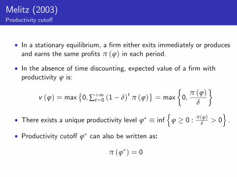
• In a stationary equilibrium, a firm either exits immediately or produces and earns the same profits π (ϕ) in each period.
• In the absence of time discounting, expected value of a firm with productivity ϕ is:
v (ϕ) = max � 0, ∑t
+=∞ 0 (1 − δ)t π (ϕ)
� = max 0,
π (δ
ϕ)
• There exists a unique productivity level ϕ∗ ≡ inf ϕ ≥ 0 : π(δϕ) > 0 .
• Productivity cutoff ϕ∗ can also be written as:
π (ϕ∗) = 0

�
Melitz (2003) Aggregate productivity
• Once we know ϕ∗, we can compute the pdf of firm-productivity levels among the active firms:
g (ϕ)
µ (ϕ) = 1−G (ϕ∗ ) if ϕ ≥ ϕ∗
0 if ϕ < ϕ∗
• Accordingly, the measure of aggregate productivity is given by: � 1 � +∞
� σ−11 �ϕ (ϕ∗) = ϕσ−1g (ϕ) d ϕ
1 − G (ϕ∗) ϕ∗

Melitz (2003) Free entry condition
• Let π ≡ Π/M denote average profits per period for surviving firms.
• Free entry requires the total expected value of profits to be equal to the fixed cost of entry:
π0 × G (ϕ∗) +
δ × [1 − G (ϕ∗)] = fe
• Free Entry Condition (FE):
δfeπ = (6)
1 − G (ϕ∗)
• Holding constant the fixed costs of entry, if firms are less likely to survive, they need to be compensated by higher average profits

� �
Melitz (2003) Zero cutoff profit condition
• Definition of ϕ∗ can be rearranged to obtain a second relationship between ϕ∗ and π.
• By definition of π, we know that
π = Π/M = π [�ϕ (ϕ∗)] π = fr [�ϕ (ϕ∗)] − 1⇔
σf
• By definition of ϕ∗, we know that
π (ϕ∗) = 0 r (ϕ∗) = σf⇔
• Two previous expressions imply ZCP condition: � r [�ϕ (ϕ∗)]
� ���ϕ (ϕ∗) �σ−1
�
π = f − 1 = f − 1 (7)r (ϕ∗) ϕ∗

Melitz (2003) Closed economy equilibrium
�
Melitz (2003) Aside: the shape of the ZCP schedule
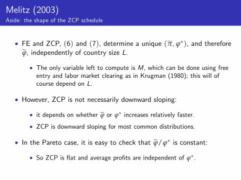
• FE and ZCP, (6) and (7), determine a unique (π, ϕ∗), and therefore ϕ, independently of country size L.
• The only variable left to compute is M, which can be done using free entry and labor market clearing as in Krugman (1980); this will of course depend on L.
• However, ZCP is not necessarily downward sloping:
• it depends on whether �ϕ or ϕ∗ increases relatively faster.
• ZCP is downward sloping for most common distributions.
• In the Pareto case, it is easy to check that �ϕ/ϕ∗ is constant:
• So ZCP is fiat and average profits are independent of ϕ∗.

Melitz (2003) Number of varieties and welfare (and openness to free trade)
• Free entry and labor market clearing imply
L = R = rM
• We can rearrange the previous expression
L LM = =
r σ (π + f )
• Like in Krugman (1980), welfare of a representative worker is given by
1 U = 1/P = M σ−1 ρ�ϕ
• Since �ϕ and π are independent of L, growth in country size (or openness to free trade) will also have the same impact as in Krugman (1980):
• welfare � because of � in total number of varieties in each country

1
2
1
2
Today’s Plan
Introduction to “New New” Trade Theory
Melitz (Ecta, 2003)
Closed economy.
Open economy with variable and fixed trade costs.

1
2
Melitz (2003) Open economy model
• In the absence of trade costs, we have seen that trade integration does not lead to any intra-industry reallocation (ie �ϕ is fixed).
• In order to move away from such (counterfactual) predictions, Melitz (2003) introduces two types of trade costs:
Iceberg trade costs: in order to sell 1 unit abroad, firms need to ship τ ≥ 1 units.
Fixed exporting costs: in order to export abroad, firms must incur an additional fixed cost fex (information, distribution, or regulation costs) after learning their productivity ϕ.
• In addition, Melitz (2003) assumes that c = 1, ..., n countries are symmetric so that wc = 1 in all countries.

Melitz (2003) Production
• Monopoly pricing now implies:
1 τ pd (ϕ) = , px (ϕ) =
ρϕ ρϕ
• Revenues in the domestic and export markets are:
rd (ϕ) = Rd [Pd ρϕ]σ−1 , rx (ϕ) = τ1−σRx [Px ρϕ]σ−1
• Note that by symmetry, we must have:
Pd = Px = P and Rd = Rx = R
• Let fx ≡ δfex . Profits in the domestic and export markets are:
πd (ϕ) = rd (ϕ) − f , πx (ϕ) =
rx (ϕ) − fxσ σ

� �
� �
� �
Melitz (2003) Productivity cutoffs
• Expected value of a firm with productivity ϕ is:
v (ϕ) = max � 0, ∑t
+=∞ 0 (1 − δ)t π (ϕ)
� = max 0,
π (δ
ϕ)
• But total profits of are now given by:
π (ϕ) = πd (ϕ) + max {0, πx (ϕ)}
Like in the closed economy, we let ϕ∗ ≡ inf ϕ ≥ 0 : π(ϕ) > 0 .•δ
In addition, we let ϕx ∗ ≡ inf ϕ ≥ ϕ∗ : πx
δ (ϕ) > 0 be the export •
cutoff.
• In order to have both exporters and non-exporters in equilibrium, ie ϕ∗ > ϕ∗, we assume that: x
τσ−1fx > f

Melitz (2003) Selection into exports
-
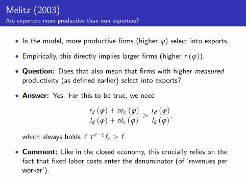
Melitz (2003) Are exporters more productive than non exporters?
• In the model, more productive firms (higher ϕ) select into exports.
• Empirically, this directly implies larger firms (higher r (ϕ)).
• Question: Does that also mean that firms with higher measured productivity (as defined earlier) select into exports?
• Answer: Yes. For this to be true, we need
rd (ϕ) + nrx (ϕ) rd (ϕ) ld (ϕ) + nlx (ϕ)
> ld (ϕ)
,
which always holds if τσ−1fx > f .
• Comment: Like in the closed economy, this crucially relies on the fact that fixed labor costs enter the denominator (of ‘revenues per worker’).
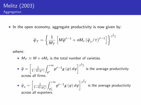
Melitz (2003) Aggregation
• In the open economy, aggregate productivity is now given by: � � �� 1 �ϕT = M1
TM �ϕσ−1 + nMx (�ϕx /τ)σ−1 σ−1
where:
• MT ≡ M + nMx is the total number of varieties. � � � 1 �ϕ = 1 +∞
ϕσ−1g (ϕ) d ϕσ−1
is the average productivity • 1−G (ϕ∗ ) ϕ∗
across all firms. � � +∞ �
σ−11 �ϕ = 1 ϕσ−1g (ϕ) d ϕ is the average productivity • x 1−G (ϕx
∗) ϕ∗x across all exporters.

Melitz (2003) Aggregation
• Once we know �ϕT , we can still compute all aggregate variables as:
1
P = MT 1−σ /ρ�ϕT ,
R = MT r (�ϕT ) ,
Π = MT π (ϕ�T ) , σ
Q = MT σ−1 q (�ϕT )
Comment:• • Like in the closed economy, there is a tight connection between welfare (1/P) and average productivity (�ϕT ).
• But in the open economy, this connection heavily relies on symmetry: welfare depends on the productivity of foreign, not domestic exporters.

Melitz (2003) Free entry condition
• The condition for free entry is unchanged.
• Free Entry Condition (FE):
δfeπ = (8)
1 − G (ϕ∗)
• The only difference is that average profits now depend on export profits as well:
π = πd (�ϕ) + npx πx (�ϕx ) where:
px = 1−G (ϕx ∗) is probability of exporting conditional on successful •
entry. 1−G (ϕ∗)

Melitz (2003) Zero cutoff profit condition
• By definition of the cut off productivity levels, we know that:
πd (ϕ∗) = 0 rd (ϕ
∗) = σf⇔
πx (ϕx ∗ ) = 0 ⇔ rx (ϕx
∗ ) = σfx
• This implies: � � 1 rx (ϕ∗ ) fx fx σ−1
x = ϕ∗ = ϕ∗τ rd (ϕ∗) f
⇔ x f
• By rearranging π as a function of ϕ∗, we get a new ZCP condition: �� �σ−1 � �� �σ−1 � �ϕ (ϕ∗) �ϕx (ϕ∗)π = f − 1 + npx fx − 1
ϕ∗ ϕ∗ (ϕ∗)x
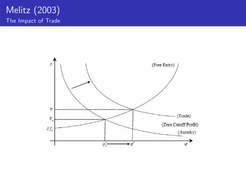
Melitz (2003) The Impact of Trade

Melitz (2003) The Impact of Trade
• In line with empirical evidence, exposure to trade forces the least productive firms to exit: ϕ∗ > ϕa
∗.
Intuition:• • For exporters: Profits � due to export opportunities, but � due to the entry of foreign firms in the domestic market (P �).
• For non-exporters: only the negative second effect is active.
Comments:• • The � in ϕ∗ is not a new source of gains from trade. It’s because there are gains from trade (P �) that ϕ∗ �increases.
• Welfare unambiguously � though number of domestic varieties �
R LM = = < Ma r σ (π + f + px nfx )
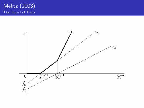
Melitz (2003) The Impact of Trade

Melitz (2003) The Impact of Trade
1
2
3
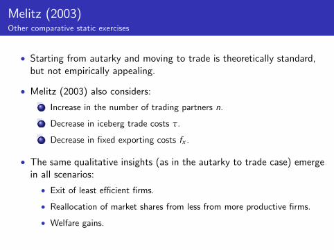
Melitz (2003) Other comparative static exercises
• Starting from autarky and moving to trade is theoretically standard, but not empirically appealing.
• Melitz (2003) also considers: Increase in the number of trading partners n.
Decrease in iceberg trade costs τ.
Decrease in fixed exporting costs fx .
• The same qualitative insights (as in the autarky to trade case) emerge in all scenarios:
Exit of least effi cient firms.•
• Reallocation of market shares from less from more productive firms.
• Welfare gains.
MIT OpenCourseWare http://ocw.mit.edu
14.581 International Economics I Spring 2011
For information about citing these materials or our Terms of Use, visit: http://ocw.mit.edu/terms.