Temporary trade and heterogeneous firms∗

Gábor Békés and Balázs MuraközyInstitute of Economics, HAS Budapest

19 December 2011

Abstract

Using Hungarian firm-transaction level export data, we show thatabout one third of firm-destination and about one half of firm-product-destination export spells are short-lived, or temporary, each year. This isin odds with theories where comparative advantage is stable and marketentry costs are sunk. We show how endogenous choice between variableand sunk cost trade technologies can explain the empirical importance andsome characteristics of temporary trade. We build a model in which thelikelihood of temporary trade depends on productivity and capital costof the firm as well as well-known gravity variables of destinations. Thesepredictions are borne out by the data; the likelihood of permanent trade,defined by a simple filter, rises with firm productivity, financial stability,proximity and GDP of destination countries.

Keywords: export, Hungary, trade instability, fixed costJEL: D40, F12CEFIG Working Paper 6, 2011 (new version)

1 Introduction

Most trade theories predict a stable export activity once comparative advantagejustifies it or once the sunk cost of such an activity is paid for. In particular,models of firm heterogeneity building on Melitz (2003) assume the existence ofa sunk cost related to the start of exporting. In extensions of the basic model 1 ,

∗Corresponding author: Balazs Murakozy: IE-HAS, 1112 Budaorsi ut 45, Budapest,Hungary. Email: murakozy@econ.core.hu. Acknowledgements: We wish to thank PeterHarasztosi for excellent research assistance. We are grateful for comments by GianmarcoOttaviano, Laszlo Halpern, Miklos Koren, Giulia Felice, Stefan Boeters and seminar partic-ipants in ERWIT/EFIGE Nottingham, ETSG Copenhagen, EEA Oslo, Uni Perugia, CEUBudapest, CPB Hague, IfW Kiel, Uni Bocconi. The authors gratefully acknowledge financialassistance from the European Firms in a Global Economy: Internal policies for external com-petitiveness (EFIGE)’, a collaborative project funded by the European Commission’s SeventhFramework Programme (contract number 225551). This work is part of the "Center for Firmsin the Global Economy (CEFIG)" network. The entire responsibility for errors and omissionsremains on us.

1Such as Helpman et al. (2004), Chaney (2008) Das et al. (2007), Arkolakis (2010), Eatonet al. (2011), Alessandria and Choi (2010)

1

sunk costs of exports are related to the export of certain products and to certaindestinations. As this sunk cost is an investment that can only be recovered froma stable stream of revenues, firms are expected to export a given product to agiven destination over a long period of time. In a simple dynamic interpretationof static sunk-cost based trade models, only dramatic shifts in demand or factorprices would lead to a halt of an export project.However, firms often export their products to a given destination for a short

period or in a series of short spells. We will call these unstable relationshipstemporary trade, while stable trade relartionships will be classified as permanenttrade.In our data for Hungary, about half the firm-destination-product specifictransactions is temporary in nature. Moreover, temporary trade appears atthe firm level as well; about a fifth of firms who ever sell abroad will exportin a temporary fashion only. Despite their high share in terms of number ofrelationships, we found that temporary trade transactions are typically muchsmaller in value than permanent trade; depending on the level of aggregationused, temporary transactions worth about 2-10% of total exports.This paper aims at putting unstable trade transactions in the limelight and

endeavors to reconcile theory with evidence. We show new evidence regardingthe pervasiveness of unstable trade relationships and build a simple model toexplain the high frequency of temporary trade relationships that we see in thedata.Why do we propose studying temporary trade which accounts for a small

fraction of aggregate trade volumes? Our work can help (i) understand patternsin disaggregate trade data, (ii) distinguish between existing trade theories, and(iii) inform policy. First, the high prevalence (i.e. large number) of small andshort-lived trade flows has long puzzled the profession (e.g. Eaton et al. (2011)),and we offer a simple and intuitive explanation. Second, ignoring the choice oftrading technology can lead empirical studies to overestimate the magnitude ofsunk costs. Third, trade policy may have to focus on promoting stable relation-ships as opposed to all export activities.Using balance sheet and customs transactions data on manufacturing firms

in Hungary, we study the stability of export spells at the firm-destination andthe firm-destination-product level. We classify each firm-destination trade flowas either permanent or temporary by introducing a simple trade relationshipstability filter. Permanent trade is an uninterrupted export spell that is atleast four years long, while temporary trade can be either a short spell or anon-continuous export relationship. Temporary trade is not limited to specificindustries or markets, and all types of firms trade temporarily over time.To explain the prevalence of temporary trade flows observed in our data, we

build a model of heterogeneous firms, extending the proposition of heterogeneityin entry costs at the firm level or demand at the country level. We model howfirms, facing uncertainty in terms of their future productivity, may endogenouslychoose between two different trade technologies. They may pay a large fee - sunkcost - up-front in return for lower costs later, or pay less now but more in eachfuture period. The endogenous choice between variable- and sunk-cost tradetechnologies can yield, for some firms and destinations, an equilibrium outcome

2

of temporary trade.This model is useful as it helps understand the seemingly erratic presence

of short spells, and provides an explanation for the small shipments present incross sectional datasets which were not well understood before. This is impor-tant as allowing firms to forgo the sunk cost of trade makes short spells quiteunderstandable - even without assuming very large and frequent productivityshocks. Hence, this model of trade technology choice will both better explainfirm export dynamics features presented in the data and offer an alternative tolearning models (e.g. Aeberhardt et al. (2009)). Furthermore, the model yieldsa number of predictions which can be matched with evidence from the data.We predict that the likelihood of permanent trade rises with firm performance,proximity and market size of destination countries.We test the specific predictions of our theory regarding determinants of tem-

porary trade, and find that our empirical results fall in line with the predictions.Using a random effect probit model, we show that the likelihood of temporarytrade rises with lower productivity, higher capital cost of the firm, greater dis-tance and larger GDP of destination countries, and that these are in line withour simple model. We extend the analysis to the firm-destination-product leveland find that product differentiation increases the probability of a permanenttrade relationship. Furthermore, we show that trade liberalization leads to anincrease of the extensive margin of both kinds of exporters, and leads to a morepositive effect on the intensive margin of permanent exporters.Our work can also inform how existing trade theories should be confronted

with the data. For example, inspired by models which assume that firms willpay an up-front sunk cost that will later be covered by export revenues, sev-eral empirical studies have estimated sunk costs of exporting to be significant(Bernard and Jensen (2004))2 . In fact, studies identifying sunk cost from thedifferent behavior and performance of exporting and non-exporting firms mayunderestimate the sunk cost as some exporters may have opted for the variablecost trade technology and not paid the sunk cost. Our framework can be usedto filter out temporary traders and estimate the model on those firms only thatdo pay a sunk cost.Finally, reducing trade costs for a limited period or providing one-off export

incentives may only lead to temporary exports without long term positive effects.At the same time, our model suggests that providing incentives in favor ofthe sunk cost based option is what may generate stable trade flows and longterm benefits. This matters for policy, because trade promotion spending oftentargets small firms and initially small volume export projects.This paper is organized as follows. In the section 2, we detail our dataset,

and present our definition of temporary and permanent trade relationships anddescribe the prevalence of temporary trade. Section 3 introduces the model

2 In a simulation of their model on French data, Eaton et al. (2011) find that fixed coststake 59 percent of gross profit in any destination. Roberts and Tybout (1997), Lawless (2010),Moxnes (2010). Furthermore, the availability of trading at a temporary fashion without a highup-front fee offers an alternative explanation to why Eaton et al. (2011) find a large numberof small transactions in the presence of high estimated sunk costs.

3

that links temporary trade to a choice of trade technology. Section 4 introducesthe evidence on temporary trade patterns and an extension to firm-destination-product level is discussed in 5. The last section concludes.

2 Data and description of temporary trade

This section first introduces our proposed trade relationship stability filter. Af-ter briefly presenting the dataset, we use our filter to show the prevalence oftemporary trade in terms of number of transactions, volume and dynamics overtime.

2.1 What is temporary trade?

The study of temporary trade is most closely associated with analyses on shortspells in trade. Some recent empirical papers emphasize the importance ofshort term relationships - mostly at a bilateral level. These relationships arenot only characteristics of small markets, like Hungary or Colombia but also oflarge economies such as the US and Germany. Besedes and Prusa (2006), forexample, show that the median duration of exporting a product is between twoand four years in the United States. Similarly, Nitsch (2009) shows that the samephenomenon can be observed in Germany - the majority of trade relationshipsexists for only one to three years. Eaton et al. (2011) look at firm-level tradeflows in Colombia, only to find a large importance of one-time exporters. Hessand Persson (2010), looking at the duration of EU imports at bilateral tradedata, find that even at national level, a large share of trade relationships areshort lived, and some stability in importing a product masks shifts in sourcecountries. Focusing at the product level Bernard et al. (2010) demonstratesthat in 1997, about quarter of output by stable (producing at least between1992 and 2002) firms comes from newly (within five years) added products andanother quarter of products will be lost within 5 years.Instead of looking at the duration of an export spell or churning of prod-

ucts, our aim is to classify each firm-destination trade flow in a year as eitherpermanent or temporary. To do that we introduce a simple trade relationshipstability filter, which will enable us to analyze the determinants of temporarytrade. The filter works as follows.First let us denote the value of a trade flow by firm i to market k at year t

as Rtik. Let t = t0 be the base year in which we would like to classify the activetrade relationships, i.e. those firm-destination combinations for which Rt0ik > 0.For each such i, k combination one can define a spell, St0ik , which denotes thenumber of consecutive years, including t, for which firm i exported to market k.Thus, if Rt0−2ik = 0;Rt0−1ik > 0;Rt0ik > 0 and Rt0+1ik = 0, then St0ik = 2. Based onthis, we say that firm i exports to market k in a permanent way if St0ik > θ, andthe export flow is temporary whenever St0ik ≤ θ, where θ is a positive integer. Inpractice, θ may represent a period long enough to include some longer than oneyear trade flows but short enough not to include stable trade relationships.

4

While this approach is arbitrary to some extent, we find it quite useful andstraightforward. It enables one to classify all trade flows in a cross section,and explain whether a flow is temporary by binary dependent variable meth-ods. We consider this as a more natural framework of analysis than for examplemodelling the length of the spells with duration models because of three rea-sons. First, as we will argue in the theory section, temporarily exporting firmsmay have chosen endogenously a different trading technology than permanentexporters, which motivates a binary rather then a continuous framework withrespect to time when modelling trade spells. Second, in duration modelling thechoice of the time period is a delicate issue: using all spells within a period, forexample, may lead to over-representation of short spells and various truncationproblems. Third, the interpretation of the results from our approach is quitestraightforward: the marginal effect shows how the probability that the flow ispermanent changes when the explanatory variable changes.In this paper, we will report most results with θ = 3, i.e. we require a

permanent trade flow to last at least four years. Note that for this exercise towork one needs data for years between t0 − θ and t0 + θ, because this enablesone to be sure whether each flow is at least θ + 1 year long. In this way, as wehave trade data until 2003, we will classify all trade relationships in t0 = 2000into either the temporary or permanent category. The choice of this year wasmotivated by the fact that post-communist transition and the most importantstructural changes in Hungarian economy already took place before 1997, thusthe observed dynamic nature of trade relationships is not a consequence oftransition. At the same time, this is an interesting period in time featuring agradual European integration process and a dynamic export-led growth.On the choice of the time window, four years of consecutive exporting is long

enough to be considered as permanent - in line with the results of Besedes andPrusa (2006), who estimate the duration of trade relationships and find thatthe survival rates decrease rapidly in the first 4-5 years (to about 45-50%), andremain reasonably stable afterwards. We consider this definition of temporarytrade relationship quite conservative. We have also experimented with otherdefinitions, in which temporary trade was somewhat more prevalent3 .Also, the method can be easily extended, with appropriate indexing, to other

levels of aggregation: the bilateral level, the firm level or the firm-product-destination level. In each case, one can classify all cross-sectional units in yeart0 based on the length of their respective spells.

2.2 The dataset

The dataset covers all export data from Hungary, for the 1992-2003 period. Thedata is structured at a firm-product-destination level with one observation inthe database being the export of a product j by firm i to country k in year t.

3According to an alternative definition, temporary trade is defined as a trade relationship,in which we can observe at least 1 positive value in a given 4-year period, but the cell isnot active for all four years. With this definition, 20-30 percent more relationships will beclassified as temporary. Results available on request.

5

The sample is long enough so that years that are pinned down for analysis (1995,2000) are followed by (at least) three years in sample as well as preceded by atleast three years. This creates a potentially balanced sample, where entry/exitobserved in the dataset is only generated by entry/exit from exporting.The dataset comes from a merger of two sources. Firm level balance sheet

and income statement data by APEH, the tax authority. Transaction level datacomes from the Customs statistics and contains information on transaction valueand quantity. This dataset consists of manufacturing firms and manufacturingproducts only. Thus, all information is related to direct export by a manufac-turing firm. The values of export are calculated as free on board.The product dimension of the dataset is disaggregated; it is broken down

to 6-digit Harmonized System (HS) level. We define a product as a 6-digitcategory, although using more aggregated (4-digit) categories does not changeour results. "Motor cars and vehicles for transporting persons" is an examplefor a 4-digit category, while "Other vehicles, spark-ignition engine of a cylindercapacity not exceeding 1,500 cc" is an example of 6-digit category.Data covers exports for 169 countries and over 700 HS6 product categories.Note that the Hungarian trade structure is close to EU countries as described

in Mayer and Ottaviano (2008) even if the concentration and role of large firmsis slightly higher in Hungary than in most EU countries. Hungary is one ofthe most open EU countries in terms of the number of trading firms and tradedvolume4 . Certain aspects of the data are comparable to previous findings on USand some European data (Baldwin and Harrigan (2011), Mayer and Ottaviano(2008)) These similarities with other countries suggest the generality of ourfindings.

2.3 Properties of temporary trade

This section will introduce some key description of the importance of temporarytrade regarding both its prevalence and volume and consider some key issues ofdynamics over time. In all three points, our results are based on using the traderelationship stability filter on Hungarian data.First, we have calculated the prevalence i.e. the (unweighted) share of

temporary trade flows in terms of number of relationships, which we present inTable 1. The main result is that about 32 percent of firm-destination exportrelationships was temporary in 2000. The share of temporary trade is even largerat the firm-product-destination level: 56.5 %.5 This shows that temporary tradeis not a curiosity: it is a robust fact of international trade.Because our definition is arbitrary to some extent, we have conducted a num-

ber of checks which confirmed that the share of temporary trade is similar when4For more on the Hungarian dataset and a set of descriptive statistics regarding trading

firms, see Békés et al. (2011).5As for the 56.5% of temporary relationships, 20pp are temporary transactions in perma-

nent products, 31.5% are temporary products by permanent firms and 5% of transactions arecarried out by temporary firms. From a destination angle, the share of temporary transactionsin permanent destinations is 39% and temporary destinations by permanent firms account for13% of all transactions.

6

Description Permanent Temporary Temp. shareFirm-destinationFull sample 11650 5434 31.81%Products >10 Mn USD* 6630 2279 25.58%Destinations>10 Bn USD* 11509 5242 31.29%Only EU25 8663 3425 28.33%Only non-EU25 2987 2009 40.21%Base year: 1995 5442 3540 39.41%4 year definition 9375 5666 37.67%FirmFull sample 3809 731 16.10%Firm-product destinationFull sample 29084 37790 56.51%*Product and destination categories are defined at aggregate level.

Table 1: Number of observations

we modify the sample or the filter. Indeed, we consider robustness checks alongfour dimensions: dropping nuisance (i.e. very small) deals, dropping far-awaycountries, changing the number of years and the base year. First, if we restrictthe sample only to significant trade flows, the figure is somewhat smaller, but itis still larger than 25 percent. Second, temporary trade is highly prevalent bothin the enlarged European Union and outside it. Note, however, that tempo-rary trade is more frequent for less important trade partners. (Hungary’s mostimportant export destinations are members of the enlarged EU). Third, withθ = 4, the share of temporary trade goes up to almost 40 percent. Fourth, in1995, a period of significant structural reforms, the share of temporary tradewas even higher, 37 percent. Our estimates are conservative as we droppedfirms that did not operate at every year during the seven-year window around2000, and all these firms are intrinsically temporary traders. Thus, one mayconclude that when looking at the number of trade relationships, temporarytrade is important at every level.Second, let us consider the volume i.e. the dollar value of trade. As a general

result, we show that the export value of firms-destination flows that are part ofa temporary relationship is rather small in dollar terms. The volume of firm-destination level is just 2% of total trade volume rising to 8.4% when adding theproduct margin, too. In terms of importance, we may drop the top 1% of firms,the large multinationals which are in many respects outliers in the economy. Forinstance, motor vehicle export of a major German multinational car companyto Germany alone accounts for 11% of total Hungarian direct export volumeby manufacturing firms. Taking the top 1% of relationships out or focusingon firms with less than 250 employees, the volume by temporary exporters (atdestination level) rises to almost 4%. At the firm-destination-product level, thevolume by temporary trade relationships is 8-10%.Third, we may consider further issues related to dynamics between 1995 and

7

Description level Full sample Less than 250 employees Without top 1%Firm-destination 1.86% 4.80% 3.86%Firm-product-level 4.50% 5.36% 5.19%Firm-product-destination-level 8.42% 10.71% 10.18%

Table 2: Value of temporary transactions in USD

2000. At the firm level, 27% of temporary firms in 1995 became permanentin 2000, 13,8% remained temporary while the rest exited from trade. At firm-destination level, while the share of exit is larger, the relative importance ofbecoming permanent exporter remains similar (see Table 13 in Appendix)A simple hypothesis based on the logic of learning models, in which firms

experiment in markets or learn from exporting would posit that firms tendto enter as temporary traders initially, and then, if they are successful, theyprobably become permanent traders or exit. However, comparing two periods(in our case, 2000 and 1995), we do not find evidence for this proposition. First, alarge share (58%) of new trade relationships in 2000 is established as permanent.Second, considering exporters in 2000, new traders are about equally likely tobecome permanent traders as former (in 1995) temporary traders (58.6% vs62.8%).In terms of dynamics, the contribution of temporary trade is rather small

with regards to new trade volume generated. As shown in the decompositionof trade growth between 1995 and 2000 in Table 14 (in Appendix), exit, entryand expansion of temporary traders was responsible for just 1.5% of total tradegrowth. Exit by temporary traders is small in value, and entry of new temporarytraders will more than offset it (2.78% vs 1.37%). Note that the most importantmargin had been the entry by new permanent traders (79.85%).

3 Modelling Temporary Trade

3.1 Relating to previous literature

As argued earlier, traditional trade models overlook the possibility of unstabletrade relationship as a mass phenomenon. However, we are not the first toargue that as firms face uncertainty, their trading activity may not be stable;this issue was analyzed both at the firm and at the firm-product level.Most recent advances in this literature keep the basic story of Melitz (2003)

and retain the assumption of a sunk cost related to the start of exporting. Inaddition, they allow for some sort of shocks, such as productivity, or per periodfixed cost, taste changes, or political and appropriation risk. In this short review,we aim at placing our approach in a set of recent advances, looking at sourcesof instability at the firm level first followed by an overview of points raised bydestination as well as product level models.A number of recent models provide a dynamic extension of the Melitz-model.

These models introduce more than one period, a per-period fixed cost and uncer-

8

tainty in the fixed cost or productivity. In these models firms are heterogeneousin terms of productivity, and uncertainty affects firms differently according totheir selected feature.A basic source of uncertainty is related to firms’overall productivity stem-

ming from human resources, technology or a change in the behavior of com-petitors. Such a shock would affect the firm’s general conduct, its decision toenter or exit foreign (or even domestic) markets. A similarly important sourceof uncertainty is shocks to the per-period fixed cost. In dynamic extensions ofthe Melitz model, this may be equivalent to a shock to firm productivity. Forinstance, in Segura-Cayuela and Vilarrubia (2008), firms pay a per period fixedcost, calculate the value of entry (into an export market) and decide. Here,given the option of waiting, higher uncertainty leads to fewer firm entries. Al-though not explicitly modelled in the paper, exit would take place if a shockto productivity is so large that it makes future payments of per period fixedcosts unlikely to be profitable. In Arkolakis (2010), different firms will choosedifferent marketing strategies owing to optimal value of marginal cost relatedto marketing spending which is negatively related to the number of additionalconsumers reached.Firm-destination level trade dynamics may be modelled in a similar way. If

uncertainty is modelled by a shock to the iceberg trade cost (i.e. ad valoremand not per period fixed costs), exit can also happen and it may be destination-specific. In line with this approach, Crozet et al. (2008) suggest that volatilemacroeconomic background (such as the exchange rate) will create large shocks,and some previously profitably exporting firms will suddenly exit. As exchangerate or political shocks are country specific, this type of uncertainty will un-equally affect a firm’s export to different countries.A second class of models derives trade dynamics from asymmetric informa-

tion or incomplete contracts rather than uncertainty about costs.If the attributes of a trading partner cannot be observed by an exporter

when they first meet, it can be optimal to ’test’potential foreign partners bystarting small. In the learning model of Rauch and Watson (2003), new entrantsshould only continue the relationship if the potential partner successfully stoodthis test. In this spirit, Besedes (2006) shows that initial size, risk and searchcosts play an important role in determining the duration of a trade relationship.Higher reliability and lower search costs lead to larger initial transactions andlonger duration. Furthermore, Araujo and Ornelas (2007) argue that in thepresence of incomplete contracts, starting in small makes sense, as it is a goodway to uncover reliability.In Aeberhardt et al. (2009) exporting requires the presence of a local distrib-

utor in each market, and it takes time to learn about the quality of distributors.Thus, the size of an export shipment of a firm to a destination grows as therelationship matures. In this model with learning, persistence is a consequenceof informational friction (i.e. lack of knowledge about distributors) rather thansunk costs. This approach de facto allows firms to invest less in the beginningand pay at every level once the reliability of distribution channel is revealed -i.e. there is a trade-off between the sunk cost and per-period costs.

9

Yet another approach is to consider firms being heterogeneous in terms ofcost structure. Differences in cost structure was endogenized in Arkolakis (2010),where firms may choose a marketing technology in a framework where costlyadvertising is needed to reach more and more consumers. In Arkolakis andMuendler (2010), firms first incur a broad market-entry cost and then an addi-tional fixed product-entry cost that is in line with the magnitude of the partic-ular overseas presence. Furthermore, these are related to product distribution(wholesale, storage, transportation, retail, etc.) in given markets. If the mar-ginal cost of adding a product in an already overtaken market is small, such acost structure may lead to high churning. In Eaton et al. (2011, p. 1454), fixedcost both depends on a firm (product)-destination specific shock and destinationspecific component which is common to all producers.So far we have only discussed firm-specific shocks while evidence from sev-

eral countries suggests a majority of export shipments being carried out bymultiproduct firms6 . Temporary trade at the firm-product level may come fromshocks, which are related to products and not result in the firm quitting fromexporting altogether.Multiproduct firm models extend the logic of dynamic Melitz models to

the firm-product level. In Bernard et al. (2010) each firm decides both entryand exit as well as in which product markets to participate. Firms enter byincurring a sunk entry cost and observe both their firm level initial productiv-ity, product-firm specific consumer taste parameters (also called expertise). Inthis framework, TFP raises the probability of producing yet another productand therefore, a firm’s product range is increasing in its productivity. At thesame time, TFP also determines overall profitability and hence entry and exitwith taste determining only the composition of the traded bundle. Bernardet al. (2011) extend their earlier model and allow for country-specific productattributes that vary across both products and countries.Another consequence of product or destination related shocks is the possi-

bility of sequential exporting as in Albornoz et al. (2010). In this model oflearning, a firm’s success in foreign markets is uncertain, but correlated acrossdestinations. This setup explains starting small as well as high exit rates of newexporters and, importantly, the rapid expansion of new destinations of survivingfirms. It implies that the likelihood of not exiting a market is correlated withnot exiting another one.Another angle is offered by Mayer et al. (2010), where firms export a product

mix based on their productivity. In conjunction with Eckel and Neary (2010),firms rank their products by their competence, and shocks as well as competitionwill affect product mix in an orderly rather than a random fashion. For ourperspective this means that there is likely to be a set of products that areexported in a rather stable manner and another set of volatile mix of products(or product-destination) further away from core competency.Overall, our approach combines the basic world view behind dynamic Melitz-

6For EU evidence, see Mayer and Ottaviano (2007), for US evidence see Bernard et al(2007). For descriptive statistics on multi-product firms in Hungary, see Békés et al. 2011.

10

type models with endogenous trade technology choice. In our case firms areheterogeneous and they face uncertainty in terms of their future productivityand they may choose from two trading technologies, paying a large fee - sunkcost - up-front in return for lower costs later or paying less now but more atevery period. This model of trade technology choice will both better explain firmexport dynamics features presented in data and offer an alternative to learningmodels.

3.2 A simple dynamic model

In this section we present a simple model to illustrate the idea of two types oftrading technologies. Our aims with this model are twofold. First, it illustratesthat short term exports may differ qualitatively from longer term exports be-cause firms exiting in the short run are more likely to use a technology we defineas variable cost trading technology. Second, the model illustrates that gravityaffects the choice of trading technologies: on larger markets a given firm is morelikely to choose what we define a sunk cost trade technology.We use a number of simplifying assumptions to make the model as tractable

as possible. Firms from the (small) home country develop a product, and maketheir export decision, and we focus on a cohort of firms which starts exportingin a given period. We assume that firms which develop the new product in eachperiod can enter the export market freely in latter periods to exclude real-optionvalue calculations.In the model, firms are heterogeneous with respect to their productivity (or

ability): firm i has a productivity φi, which is firm-specific but is common to allmarkets of the firm i. Countries are indexed by k = (1...K) and are endowedwith Lk units of labour that are supplied inelastically with zero disutility. Therepresentative consumer in each country derives utility from the consumptionof a continuum of l products that we normalize to the interval [0; 1]. Consumershave the traditional CES utility for the products.Consumption of goods in country k is a CES function of goods produced by

all countries’firms. There is monopolistic competition a la Dixit and Stiglitz(1977), and the equilibrium price of a product variety is a constant mark-upover marginal cost. Cost in turn depends on both firm ability and transportcost to the destination country k, τ ik. Our model follows an export decision ofa firm, i.e. starting to sell the product to a new market. The net revenue forfirm i from supplying country k is

rk(φi, τ ik) = (τ ik)1−σwkLk(ρPkφi)σ−1 (1)

where σ = 1/(1−ρ) is the elasticity of substitution across varieties, Lk is sizeof labour force in the destination country, wk is the wage level in the destinationcountry and Pk is the price index of destination country7 . We can assume that

7Most models assume the probability of an external "death by force majeure events"independent of productivity or attribute. Here we only consider firms that operate throughoutour period of interest and hence, disregard this option. Note that introducing such an optionwould not change results.

11

firm ability is distributed according a Pareto distribution with parameters m0

and κ > 1. For tractability, we also introduce ϕi ≡ φiσ−1.First we will describe the decision of firm i whether to export to market k.

For brevity, we will omit the destination country index, but we will index thevariables which may change in time by t.Our model has three periods. In period 1, a firm decides whether to start

exporting, picks one of the two available export technologies, and receives prof-its accordingly. At periods 2 and 3, the firm may decide to continue or haltexporting; we interpret period 2 as the short-term period and period 3 is thelong-term period.At the beginning of each period, firms face stochastic shocks to their pro-

ductivity: with probability p, their ϕ increases with a factor of d > 0, thusϕit+1 = dϕit, and with probability 1 − p productivity falls in a similar pro-portion: ϕit+1 = 1

dϕit. We also assume that firms discount their profits withδ1 > 0 and δ2 > 0 in period 2 and 3, respectively. (As periods can have adifferent expected length - i.e. long-term is likely to be longer than the shortterm -, we opted for this general approach rather than a more traditional useif δ and δ2.) We assume that, while the model is stochastic, all parameters arecommon knowledge for all firms.In the first period firms may choose between two trading options called

variable cost trade (VCT) technology and sunk cost trade (SCT) technology.Both kinds of firms have to pay a fixed cost in every period, which is normalizedto 1. The sunk cost technology also requires an up-front sunk cost investmentin period 1, S > 0, and its advantage is a low transportation cost, τ . VCTtechnology firms, on the other hand, do not have to pay a sunk entry cost, butthey do not have an established network, which results in larger transportationcost: it is (χ

1σ−1 )τ , where χ > 1, and χ

1σ−1 > 1. Note that we assume that the

transport cost depends on the elasticity of substitution across varieties, which,in this simplest form of the model, is just a constant. In the model extension insection 5, we will elaborate on the rationale for this formula.For simplicity, we assume that SCT firms, which have paid the sunk cost,

can always export with a transport cost of τ in period 3, even if the firm doesnot export in period 2. We also assume that compared to the stochastic shock,the transportation cost advantage is not too large: d > χ.

As it was shown previously, the export revenue of a firm, whenever it ex-ports, is a function of ϕit and the chosen trade technology. When exportingwith VCT technology, the revenue of the firm is determined by: RSCT (ϕit) ≡rk(φit, χ

1σ−1 τ) = 1

χ (τ)1−σwkLk(ρPk)σ−1ϕit. As now we only consider the prob-lem of firms on a specified market, we will denote R ≡ 1

χ (τ)1−σwkLk(ρPk)σ−1,and hence,

RV CT (ϕit) = Rϕit (2)

Note that RV CT (ϕit) is a positive linear function of ϕit. Also, revenue withSCT technology is higher than with VCT :

12

Figure 1: State of nature tree for VCT. RV,1 is revenue of VCT firm at firstperiod.

RSCT (ϕit) = χRϕi1 (3)

In what follows, we assume that sunk and fixed costs are constant acrossmarkets, while it follows from our specification that RSCT (ϕit) and R

V CT (ϕit)are increasing in market size. Finally, for simplicity, we assume that firmschoose to export when doing it leads to a profit of 0, and choose the sunk-cost technology whenever they are indifferent between the two kinds of exporttechnologies.Figure 1 shows an example for the mechanics of our model for VCT technology-

type firms with initial productivity just above the per period fixed cost. Inperiod 1, the firm observes its initial productivity ϕi1, from which it calculatesits RV CT (ϕi1) or RV,1 for short. The firm will export in this period if this islarger than 1 (denoted by the dash line in the figure), with a first period profit ofπV CTi1 = Rϕi1 − 1. In period 2, the firm will receive a shock: with probability pits export revenue increases to dRϕi1 and with probability 1−p, it will decreaseto 1

dRϕi1. As, the revenue in this latter case is below 1, the firm will exportonly after a positive shock in period 2 - as shown in the figure with revenuebeing below the dashed line. If, following a second period positive shock, thefirm receives a positive shock in the third period as well, its potential exportrevenue will increase to d2Rϕi1 with probability p, and fall back to Rϕi1 withprobability 1 − p; it will export in both cases. After a negative shock in thesecond period, on the other hand, it will only export after a positive first-periodshock.An important consequence of this setup is that the probability of exporting

in different periods and the expected export profit only depends on the value ofϕi1. If, as in Figure 1, 1 ≤ Rϕi1 < d, the firm will export with probability 1 in

13

Figure 2: State of nature tree for SCT. RS,1 is revenue of SCT firm at firstperiod.

period 1, p in period 2 and p2 + p(1− p) in period 3. Also, its expected profit,EΠV CT (ϕi1), is the discounted sum of expected profits in the three periods. If,however, initial productivity is somewhat larger, e.g. d ≤ Rϕi1 < d2 (whichwould mean that export revenue from initial productivity is higher relative to1), it will become profitable to export even after a bad shock in the secondperiod, and the firm will only exit in the third period after two bad shocks.For firms opting for the SCT technology, the setup is similar, save that they

pay a sunk cost in the beginning but the threshold of exporting becomes loweras their net revenue is higher for a given productivity level8 . This is shown forthe same firm in Figure 2 with first period revenue of RSCT (ϕi1) or RS,1 forshort. Note that while the fixed cost is unchanged, revenues are higher in theSCT case as defined in (3).In what follows, we characterize the behavior of VCT and SCT-type firms,

then show how firms choose the export technology and finally we formulate somepredictions.

8The model could be made explicitly dynamic (i.e. allowing firms to change their statusat some point) by substantial complications only. While this is subject to further research,let us refer the readers a set of different models (Buono et al. (2008), Albornoz et al. (2010)or Morales et al. (2011)) highlight dynamic aspects of moving around export markets as wellas becoming permanent while being temporary as well. Ruhl and Willis (2008) considersa dynamic discrete choice model with per-period market-level cost when a firm wishes tomaintain export market presence.

14

3.3 VCT technology firms

A VCT technology firm exports whenever its export revenue is not lower thanthe per-period fixed cost: Rϕit ≥ 1. We will calculate the exit rates and theexpected profitability for each ϕit to be able to predict the optimal tradingtechnology choice and the exit rate.Because of the discrete nature of the stochastic process in the model, the

expected profit is not a smooth function of ϕit. To handle this, it is usefulto classify the firms into three categories according to the first time they maystop exporting. Naturally, firms with Rϕi1 < 1 do not start exporting, andwe will not deal with them here. Second, as we have seen in Figure 1, firmswith 1 ≤ Rϕi1 < d stop exporting in period 2, as their potential export revenuemay sink under the fixed costs with probability 1 − p. Third, the potentialexport revenue of firms with d ≤ Rϕi1 < d2 is always higher than the fixedcost in period 2, but may stop exporting in period 3 after two bad shocks withprobability (1 − p)2. Finally, firms with a very high potential export revenue,i.e. Rϕi1 ≥ d2 always export in all three periods.To derive the expected profit from exporting, consider a firm for which 1/R ≤

ϕi1 < d/R. The export revenue of this firm is the discounted sum of exportrevenues in all periods and states of the world:

EΠV CT (ϕi1) = ARϕi1 −B (4)

whereA =[1 + δ1pd+ δ2p

2d2 + δ2p(1− p)]andB =

[1 + δ1p+ δ2p

2 + δ2p(1− p)].

Consider now a firm with higher productivity, where d/R ≤ ϕi1 < d2/R.This firm may only exit in the long run; and hence, the expected export profitincludes the second period revenue even after a bad shock before the secondperiod:

EΠV CT (ϕi1) = ARϕi1 −B + δ1(1− p)(

1

dRϕi1 − 1

)(5)

Note that the function is continuous in ϕi1 = d/R, because in that point thefirm is indifferent in period two after a bad shock.Finally, firms with the highest productivity always export. Accordingly,

their expected profit is

EΠV CT (ϕi1) = ARϕi1−B+δ1(1−p)(

1

dRϕi1 − 1

)+δ2(1−p)2

(1

d2Rϕi1 − 1

)(6)

This function is also continuous when ϕi1 = d2/R. Also, EΠV CT (ϕi1) is(weakly) convex in ϕi1, as an increase in ϕi1 has two positive effects: exportis profitable in more states of nature, and the profit increases from alreadyprofitable states of nature.

15

3.4 SCT technology firms

The problem of SCT technology firms is very similar to VCT-type firms:

EΠSCT (ϕi1) =

χARϕi1 −B − S if 1

χR ≤ ϕi1 <dχR

χARϕi1 −B + δ1(1− p)(1dχRϕi1 − 1

)− S if d

χR ≤ ϕi1 <d2

χR

χARϕi1 −B + δ1(1− p)(1dχRϕi1 − 1

)+

δ2(1− p)2(1d2χRϕi1 − 1

)− S if d2

χR ≤ ϕi1(7)

Similarly to EΠV CT (ϕi1), this function is continuous and increasing in ϕi1.Using these functions for VCT and SCT technology firms, the following

proposition shows that when comparing two firms with the same ϕi1 but withdifferent trading technologies, the VCT technology firm is more likely to exitearlier and hence, be classified as a temporary trader.

Proposition 1 For any given ϕi1 ≥ 1/R, the probability that an SCT technol-ogy firm exit in period 2 is not larger than the probability that a VCT-type firmexits.

Proof. Let us analyze the problem for different intervals. (i) When 1R ≤ ϕi1 <

dχR , the probability of exit in period 2 for both types of firms is 1 − p. (ii) IfdχR ≤ ϕi1 <

dR , the probability of exit in period 2 for an SCT technology firm is

0, while it is 1− p for VCT-type firms. (iii) if ϕi1 ≥ dR , neither firm type exits

in period 2.

3.5 Technology choice

Naturally, a firm chooses SCT technology whenever the expected profit fromit is higher than that from the VCT, i.e. EΠSCT (ϕi1) − EΠV CT (ϕi1) ≥ 0. Tocharacterize this choice, we analyze the behavior of the left-hand side of thisequation.First, we assume that the sunk cost is large enough to ensure that it is not

profitable to export with the sunk cost technology whenever it is not profitableto export with the variable cost technology. This means, that S > χA − B.The motivation for this assumption is that otherwise VCT would clearly bedominated by SCT for all firms.One consequence of this assumption is that, when ϕi1 < 1/R, it is not prof-

itable to export at all. For larger productivity draws, the following propositionholds.

Lemma 2 When ϕi1 ≥ 1/R, the EΠSCT (ϕi1)− EΠV CT (ϕi1) function is con-tinuous and (strictly) monotonically increasing. Also, lim

ϕi1→∞EΠSCT (ϕi1) −

EΠV CT (ϕi1) =∞.

16

Proof. The continuity is the consequence of the fact that the two expectedprofit functions are continuous.The monotonicity is also intuitive. As the function is the sum of two func-

tions which are linear in different intervals, it can also be represented in sucha way. Taken into account that 1 < χ < d, the endpoints of the relevantintervals for ϕi1 are 1/χR, 1/R, d/χR, d/R, d2/χR, d2/R. Differentiating theEΠSCT (ϕi1) − EΠV CT (ϕi1) function separately for each interval, we get posi-tive derivatives for all intervals.When ϕi1 ≥ d2/R, the function is (χ− 1)A(ϕi1)+δ1(1−p)

(1d (χ− 1)Rϕi1 − 1

)+

δ2(1− p)2(1d2 (χ− 1)Rϕi1 − 1

)− S. The last term is a constant, and the first

three terms are positive and positive linear functions of ϕi1, thus the limit ofthe EΠSCT (ϕi1)− EΠV CT (ϕi1) function is ∞.The intuition behind the monotonicity property is that there are two rein-

forcing effects when ϕi1 increases. First, it becomes profitable to export in moreand more branches of the tree in Figure 1. This means that the higher the ϕi1 ofSCT technology firms, the more states of nature they can enjoy their transportcost advantage in (assuming, that they have paid the sunk cost). Second, theprofit in branches where the firm already exports increases faster with the SCTtechnology because of the lower transport cost.The result regarding the limit property of EΠSCT (ϕi1)−EΠV CT (ϕi1) comes

from the fact that the only effect of productivity increase is that profits in eachbranch increase when ϕi1 ≥ d2/R, and both types of firms export at all branchesof the tree. Because of the transportation cost advantage, SCT technology firmsbenefit more from this advantage.The main consequence of these results is that there is a cut-off value, ϕ∗i1

such that all firms below this choose the VCT technology, and firms with ahigher export revenue potential choose the SCT technology:

Proposition 3 When S > χA−B, there is a cut-off ϕ∗i1,where EΠSCT (ϕ∗i1)−EΠV CT (ϕ∗i1) = S. All firms with 1/R ≤ ϕi1 < ϕ∗i1 choose the VCT technology,and firms with ϕi1 ≥ ϕ∗i1 choose the SCT technology.

Proof. As EΠSCT (ϕi1) − EΠV CT (ϕi1) is a strictly monotonously increasingcontinuous function when ϕi1 > 1/R, also EΠSCT (1/R) − EΠV CT (1/R) < 0when S > χA − B; and lim

ϕi1→∞EΠSCT (ϕi1) − EΠV CT (ϕi1) = ∞, there should

be one and only one ϕ∗i1, where EΠSCT (ϕi1)−EΠV CT (ϕi1) = S. For ϕi1 < ϕ∗i1,EΠSCT (ϕi1) − EΠV CT (ϕi1) < 0, thus it is more profitable to choose the VCTtechnology. Conversely, when ϕi1 ≥ ϕ∗i1, EΠSCT (ϕi1)− EΠV CT (ϕi1) ≥ 0, it ismore profitable to use the SCT technology.Given the cut-off ϕ∗i1, we can calculate the share of firms entering with

either type of technologies. According to our assumption, the distribution of

φi1 = ϕ1

σ−1i1 is Pareto with parameters with m0 and κ > 1. Without loss of

generality, we can assume that m0 = 1/R1

σ−1 , the lowest productivity exporter,because we are interested in the share of SCT firms across exporters ratherthan all firms. The share of firms entering with VCT technology is nV CT =

17

F (ϕ∗ 1σ−1

i1 ) = 1 −(

1

Rϕ∗ 1σ−1

i1

)κ, and naturally the share of firms entering with

the SCT technology is nSCT =

(1

Rϕ∗ 1σ−1

i1

)κ. Using this, we can calculate

the average φi1 for both kinds of firms: it isκϕ

∗ 1σ−1

i1

κ−1 for SCT-type firms and

1/Rκ

1−(1/Rϕ

∗ 1σ−1

i1

)κ κκ−1

(Rκ−1 − 1

ϕ∗ κ−1σ−1

i1

)for VCT-type firms.

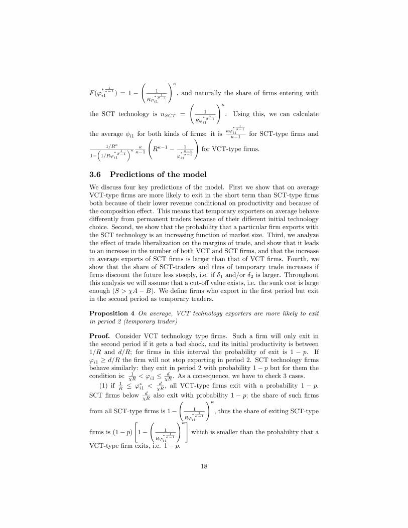
3.6 Predictions of the model

We discuss four key predictions of the model. First we show that on averageVCT-type firms are more likely to exit in the short term than SCT-type firmsboth because of their lower revenue conditional on productivity and because ofthe composition effect. This means that temporary exporters on average behavedifferently from permanent traders because of their different initial technologychoice. Second, we show that the probability that a particular firm exports withthe SCT technology is an increasing function of market size. Third, we analyzethe effect of trade liberalization on the margins of trade, and show that it leadsto an increase in the number of both VCT and SCT firms, and that the increasein average exports of SCT firms is larger than that of VCT firms. Fourth, weshow that the share of SCT-traders and thus of temporary trade increases iffirms discount the future less steeply, i.e. if δ1 and/or δ2 is larger. Throughoutthis analysis we will assume that a cut-off value exists, i.e. the sunk cost is largeenough (S > χA− B). We define firms who export in the first period but exitin the second period as temporary traders.

Proposition 4 On average, VCT technology exporters are more likely to exitin period 2 (temporary trader)

Proof. Consider VCT technology type firms. Such a firm will only exit inthe second period if it gets a bad shock, and its initial productivity is between1/R and d/R; for firms in this interval the probability of exit is 1 − p. Ifϕi1 ≥ d/R the firm will not stop exporting in period 2. SCT technology firmsbehave similarly: they exit in period 2 with probability 1− p but for them thecondition is: 1

χR < ϕi1 ≤ dχR . As a consequence, we have to check 3 cases.

(1) if 1R ≤ ϕ∗i1 <

dχR , all VCT-type firms exit with a probability 1 − p.

SCT firms below dχR also exit with probability 1 − p; the share of such firms

from all SCT-type firms is 1−(

1

Rϕ∗ 1σ−1

i1

)κ, thus the share of exiting SCT-type

firms is (1− p)[

1−(

1

Rϕ∗ 1σ−1

i1

)κ]which is smaller than the probability that a

VCT-type firm exits, i.e. 1− p.

18

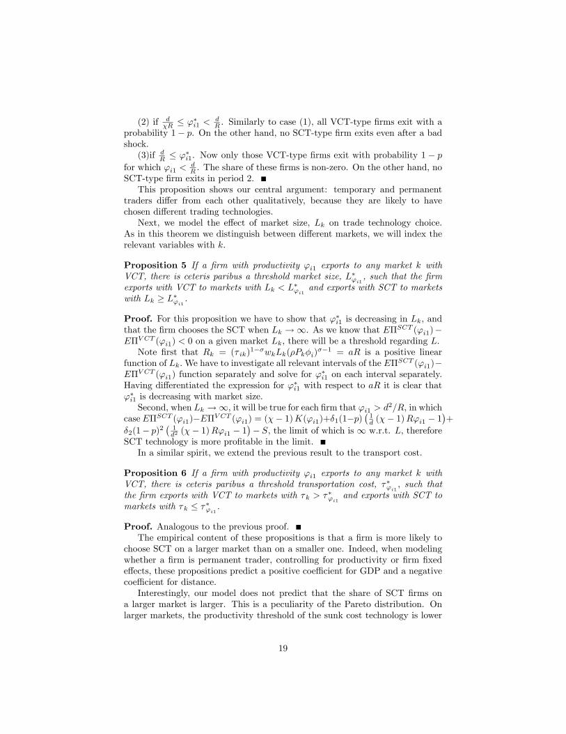
(2) if dχR ≤ ϕ∗i1 <

dR . Similarly to case (1), all VCT-type firms exit with a

probability 1− p. On the other hand, no SCT-type firm exits even after a badshock.(3)if d

R ≤ ϕ∗i1. Now only those VCT-type firms exit with probability 1 − pfor which ϕi1 <

dR . The share of these firms is non-zero. On the other hand, no

SCT-type firm exits in period 2.This proposition shows our central argument: temporary and permanent

traders differ from each other qualitatively, because they are likely to havechosen different trading technologies.Next, we model the effect of market size, Lk on trade technology choice.

As in this theorem we distinguish between different markets, we will index therelevant variables with k.

Proposition 5 If a firm with productivity ϕi1 exports to any market k withVCT, there is ceteris paribus a threshold market size, L∗ϕi1 , such that the firmexports with VCT to markets with Lk < L∗ϕi1 and exports with SCT to marketswith Lk ≥ L∗ϕi1 .

Proof. For this proposition we have to show that ϕ∗i1 is decreasing in Lk, andthat the firm chooses the SCT when Lk →∞. As we know that EΠSCT (ϕi1)−EΠV CT (ϕi1) < 0 on a given market Lk, there will be a threshold regarding L.

Note first that Rk = (τ ik)1−σwkLk(ρPkφi)σ−1 = aR is a positive linear

function of Lk.We have to investigate all relevant intervals of the EΠSCT (ϕi1)−EΠV CT (ϕi1) function separately and solve for ϕ

∗i1 on each interval separately.

Having differentiated the expression for ϕ∗i1 with respect to aR it is clear thatϕ∗i1 is decreasing with market size.Second, when Lk →∞, it will be true for each firm that ϕi1 > d2/R, in which

case EΠSCT (ϕi1)−EΠV CT (ϕi1) = (χ− 1)K(ϕi1)+δ1(1−p)(1d (χ− 1)Rϕi1 − 1

)+

δ2(1− p)2(1d2 (χ− 1)Rϕi1 − 1

)− S, the limit of which is ∞ w.r.t. L, therefore

SCT technology is more profitable in the limit.In a similar spirit, we extend the previous result to the transport cost.

Proposition 6 If a firm with productivity ϕi1 exports to any market k withVCT, there is ceteris paribus a threshold transportation cost, τ∗ϕi1 , such thatthe firm exports with VCT to markets with τk > τ∗ϕi1 and exports with SCT tomarkets with τk ≤ τ∗ϕi1 .

Proof. Analogous to the previous proof.The empirical content of these propositions is that a firm is more likely to

choose SCT on a larger market than on a smaller one. Indeed, when modelingwhether a firm is permanent trader, controlling for productivity or firm fixedeffects, these propositions predict a positive coeffi cient for GDP and a negativecoeffi cient for distance.Interestingly, our model does not predict that the share of SCT firms on

a larger market is larger. This is a peculiarity of the Pareto distribution. Onlarger markets, the productivity threshold of the sunk cost technology is lower

19

but so is the threshold for exporting at all. Because of the characteristics of thePareto distribution, the inflow of new exporters is exactly such that the shareof SCT firms remains unchanged relative to a smaller market.However, empirically it is true that the share of permanent traders is an

increasing function of market size without controlling for productivity or firmfixed effects. Our model would only provide this prediction with assuming someother productivity distribution function or ’tilting the table’ for the SCT inlarger markets, assuming for example that its transportation cost advantage isincreasing with market size.9

Based on the intuition of the previous results we may formulate a propositionabout the effect of trade liberalization on the different margins.

Proposition 7 Trade liberalization leads to an increase in the number of bothVCT and SCT exporters (extensive margin). Exports/firm (the intensive mar-gin) increases for SCT-type firms if σ > 2, and the growth of the intensivemargin is smaller for VCT-type firms than for SCT firms.

Proof. The threshold productivity of exporting, φ̂i1, (where firms are indifferentbetween exporting and exporting with the VCT) is given byA(τ ik)1−σwkLk(ρPkφ̂i1)

σ−1 ≡B. By taking logarithms of both sides and differentiating w.r.t transportation

cost yields ∂ ln φ̂i1∂ ln τ ik

= 1, thus, at the margin a 1 % decrease in transportationcost leads to a 1 percent decrease in the threshold. Similarly, differentiating thethreshold between the VCT and SCT technologies, ϕ∗i1, yields

∂ lnϕ∗i1∂ ln τ ik

= 1. Tak-ing into account the properties of the Pareto distribution, this means that thenumber of VCT and SCT firms increases in the same proportion at the marginas a result of trade liberalization.Consider now the intensive margin of SCT firms. There are two effects

here. First, all previous SCT-type firms export more by −∂ ln(τ ik)1−σ

∂ ln τ ik= (σ −

1)ε percent. Second, the threshold falls by ε = ∂ ln τ ik percent, leading to acomposition effect which has a negative effect on the intensive margin, reducingthe average productivity by ε percent. When σ = 2, the revenue is a linearfunction of productivity, hence the two effects are equal: the intensive margindoes not change. When σ > 2, however, higher productivity firms have a largerweight in average revenue than in the average productivity, thus a decrease of εin average productivity as a consequence of the change in the threshold leads toa smaller proportional decrease in average revenue. As a result, when σ > 2, theintensive margin increases as a consequence of trade liberalization - and notethat in most estimates σ is estimated to be around 510 .Consider now VCT firms. Here there is a third effect as well: the highest

productivity formerly VCT firms become SCT firms, which has a negative effect

9Another such ’trick’would be to assume that there is no transportation cost for SCT-firms. While it is a completely realistic assumption in the export vs. FDI choice in Helpmanet al. (2004), here it seems less attractive.10For example, Lai and Trefler (2002) estimates σ for several countries and models and finds

σ to be between 4.7 and 7.2.

20

on average productivity and revenues. Thus the increase in the intensive marginis smaller for VCT firms than for SCT firms.The logic of the extensive margin result is straightforward: the decrease

in trade cost makes both exporting in general and SCT trade in particularmore impressive. For small changes and Pareto distribution the number offirms exporting with both technologies increases in similar proportions. Thelogic of the intensive margin result is that for SCT-type firms, when σ is largeenough, the increase in the exports of the most productive firms is larger thanthe composition effect coming from some less productive firms switching to theSCT technology. In case of VCT firms, however, there are two compositioneffects: some less productive firms become exporters and the most productiveof these firms become SCT firms. Note, that if σ is large, it is easily possiblethat the intensive margin of these firms decreases.Finally, we turn to the question of the discount factor, and show that the

larger it is (i.e. the less steeply a firm discounts future), the higher the shareof permanent traders is. The intuition of this result is clear: the lower discountdecreases the return of investing into the SCT technology.

Proposition 8 The share of SCT-type traders is increasing in δ1 and δ2. Also,the share of temporary traders is a non-decreasing function of δ1 and δ2.

Proof. As S does not depend on the discount factors, it is enough to show that(i) EΠSCT (1/R)−EΠV CT (1/R) is smaller when the discount factors are smaller,and that (ii) the derivative of EΠSCT (ϕi1)− EΠV CT (ϕi1) is non-increasing inthe discount factors. These together mean that, with some abuse of notation,if δ1 < δ′1, for all Ri1, EΠSCT (ϕi1, δ1) − EΠV CT (ϕi1, δ1) ≥ EΠSCT (ϕi1, δ

′1) −

EΠV CT (ϕi1, δ′1), and the same is true for δ2 < δ′2. From this one can conclude

that ϕ∗i1 is a non-increasing function of the discount factors. Because of Propo-sition 1 this also means that the share of temporary traders is a non-decreasingfunction of the discount factors.(i) EΠSCT (1)−EΠV CT (1) = (χ− 1)R(1 + δ1pd+ δ2

[p2d2 + p(1− p)

])−S.

Differentiating this w.r.t. δ1 yields (χ − 1)Rpd > 0. Differentiating w.r.t δ2yields (χ− 1)R

[p2d2 + p(1− p)

]> 0.

(ii) The proof comes from calculating the derivatives of EΠSCT (ϕi1) −EΠV CT (ϕi1) for each interval.

4 Empirical evidence

The model presented earlier considers a firm starting to export and exiting basedon its technology choice and productivity shocks. However, as trade technologychoice - in contrast with trade spells - is not observable in our database, we usethe trade relationship stability filter introduced in section 2 to test predictions.This cross-section tool, based on a seven-year panel dataset, allows us to considerall trading firms and not only those who start trading at a given base year.As we have shown that there is a strong connection between trade technologychoice and the length of trade flows, we are convinced that showing that our

21

predictions describe well the difference between permanent and temporary tradewill provide empirical support to our framework.This section presents evidence regarding trade patterns. We have four pre-

dictions generated from the model.(E1) More productive firms are more likely to trade at permanent fashion,

controlling for market characteristics (Proposition 3)(E2) Trade with larger and closer markets are more likely to be permanent,

controlling for firm characteristics. (Propositions 6 and 5)(E3) Firms with higher capital cost (i.e higher discount rate) are, ceteris

paribus, more likely to trade temporary. (Proposition 8)(E4) Trade liberalization leads to increasing in extensive margins of both

kinds of exporters, and leads to a more positive effect on the intensive marginof permanent exporters. (Proposition 7)We will test these hypotheses by modelling the probability that a firm-

destination relationship is permanent in nature. We first present the empiricalstrategy based on the model outlined in the previous section. This is followedby results and some robustness checks. Finally we extend our setup to discusseffects of trade liberalization.

4.1 Empirical model

The model in the previous section allowed us making predictions regarding thelikelihood of temporary trade as a function of a set of firm, destination and firm-destination variables. We estimate the probability that a trade relationship byfirm i to country k is permanent in nature as:

Pr(Tik) = F (α+ β′Fi + γ′Mk + µi + λk + εik) (8)

where Fi refers to firm level characteristics (ability, capital cost) andMj in-cludes destination market features (size, distance), µi are firm level fixed effects,and λk are destination-level random effects.Our left hand side variable Tik = 1 if a relationship is permanent, and Tik = 0

if temporary.To investigate (8) we estimate linear probability and probit models with

destination-level random effects and different sets of fixed effects. Motivatedby the methodology in Harrigan and Deng (2008) and Mayer et al. (2010), weopt for this approach to allow for using transaction level approach as well asproduct and/or firm level fixed effects as a control for heterogeneity.In terms of measurement, productivity (or ability) is proxied by Total Factor

Productivity or TFP, firm size, export to total sales share and a dummy is usedfor multi-product firms. GDP and GDP per capita are all measured in logs at astandard fashion. Transport cost is simply measured by distance with data fromCEPII. Further, we use industry dummies at two-digit nace level. For detailson variables, see Table 7 in the Appendix.Capital cost is proxied by credit risk and we chose an index used by banks to

assess credit risks suggested by BIS (2006) and investigated by Forlani (2010).

22

The Solvency Ratio (SR) is the ratio of net assets of the firm plus long-termdebts to total assets plus leftover stock. It measures the ability of a firm toservice its debt and to accomplish long-term development11 . The higher theratio of internal and secured funding, the smaller the likelihood of paymentproblems, and hence, the lower the capital cost for the firm.

SR = Equity + Reserves + Profits +LT debtTotal Assets + Stock of goods

Another cause for lower capital cost would be sales to take place within amultinational group where the internal funding may be cheaper and the sunkcost of exporting set lower. Unfortunately, the data is unable to detect withingroup sales, i.e. when Audi Hungary exports to its German parent or anothersubsidiary in Spain. We use a foreign ownership dummy, which may be con-sidered as a proxy to presence of within group sales, and hence, should implya greater likelihood of permanent trade. Of course, foreign share being bothrelated to within group sales and cost of capital may be hardly disentangled.As introduced in section 3, firms are assumed to avoid a sudden death shock.

In terms of empirical exercise, we omitted firms who exported in 2000 but either(i) were born after 1996 or (ii) exited before 2004. Thus, all firms studied wereoperating during our 7-year window of 1997-2003. As a result, we excluded27.3% of firms which corresponds to 20.3% of relationships (for details, see Table9 in Appendix). Given that all these firms are intrinsically temporary traders,our results regarding the importance of temporary trade are conservative.Next, we present our baseline results and some robustness checks.

4.2 Results

To test predictions E1-E3, we estimated (8) using a random effect probit model.Table 3 presents the results. The first column includes the key variables, produc-tivity (TFP), credit cost (solvency ratio) as well as the gravity variables: GDP(total GDP and GDP per capita) and transport cost (distance). All coeffi cientspresented are marginal effects.Evidence is in line with model predictions. Baseline results (column 1) sug-

gest that more productive and better financed firms are more likely to tradeat a permanent level. In terms of export markets, market size (total GDP)is positively correlated with the probability to export at a permanent fashion,while high trade cost (proxied by distance) acts as hindrance. In the extendedmodel (column 2) control variables are added to better model firm ability. Size,export share and product scope (proxied by a multi-product dummy) all entersignificantly with the expected positive sign while other results hardly change.One may argue that the success of trade affects firm size or productivity,

creating a simultaneity problem. To solve this, instead of values for 2000, weused values for 1997 in the third column - with no apparent difference (column3). Finally, to test separately for firm specific or destination specific variables,

11As an alternative, in line with BIS, we used the Financial Independence Index (FII), whichis simple net assets (equity, reserves, profits) to the total assets - with no affect on results.

23

(1) (2) (3) (4) (5)VARIABLES Probit Probit Probit, Lag Lin.prob Lin.probGDP (ln) 0.119*** 0.134*** 0.119*** 0.053*** 0.071***

(0.013) (0.015) (0.013) (0.008) (0.008)GDP pcapita (ln) 0.108*** 0.100*** 0.090*** 0.018 0.022

(0.023) (0.027) (0.024) (0.013) (0.015)Distance (ln) -0.258*** -0.336*** -0.252*** -0.119*** -0.145***

(0.017) (0.021) (0.018) (0.008) (0.010)TFP 0.218*** 0.056*** 0.180*** 0.015**

(0.011) (0.013) (0.013) (0.006)Solvency Ratio 0.125*** 0.186*** 0.084*** 0.061***

(0.033) (0.035) (0.031) (0.010)Foreign-owned, D 0.085*** 0.025***

(0.025) (0.009)Export share 0.650*** 0.201***

(0.036) (0.031)No. employees 0.131*** 0.040***

(0.008) (0.002)Multi-product firm, D 0.630*** 0.232***

(0.088) (0.041)Fixed effects Nace2 Nace2 Nace2 Nace2 FirmObservations 16 660 16 633 13 674 16 633 17 084R-squared 0.05( a ) 0.09( a ) 0.04( a ) 0.12 0.09Number of dest 169 169 167 169 169log likelihood 9660 9167 7748

(a) Pseudo R squared is noted for Probit models

Robust standard errors in parentheses *** p<0.01, ** p<0.05, * p<0.1

Table 3: Firm-destination level random effect probit and linear probability mod-els, dependent variable: T=1 if relationship permanent, 0 if temporary

24

destination and firm fixed effects were introduced in a linear probability model.Results remained unchanged (columns 4 and 5).To see economic impact, we evaluate the basic probit model at sample means

(see Table 7 in the Appendix for values). At those values, the probability to be apermanent exporter is 74.4%. One standard deviation increase in productivityraises this probability by 2.4 percentage points. If the GDP of a destinationrises by one standard deviation, the probability to export there at a permanentfashion rises by 2.5 pp. Similarly, a one standard deviation increase in per capitaincome has an effect of 0.7pp.Several robustness checks have been carried out regarding firm scope, prod-

uct size and destination importance, see section 7.3 and Table 12 in the Ap-pendix. Our results were robust to excluding a large number of unimportantdestination markets, small shipments and single-product firms.

4.3 Margins of trade

In this subsection we test our predictions (E4) about the effects of trade lib-eralization. As Hungary underwent significant liberalization between 1995 and2000, we have chosen these two dates to compare the intensive and extensivemargins of permanent and temporary trade flows. For this, we simply calculatedthe number of firm-destination export flows separately for total, temporary andpermanent trade as a measure for the extensive margin, and divided total tradevolume with this to yield a proxy for the intensive margin. Table 4 present thechange in intensive and extensive margins between 1995 and 2000.The results are in line with our predictions. First, and most importantly,

the reaction to trade liberalization of temporary and permanent trade is differ-ent. Second, both extensive margins increased, but this increase was larger forpermanent trade. (While our model predicted both temporary and permanentextensive margins to increase, it does not predict a greater increase of tempo-rary trade; this may be a consequence of the Pareto distribution function, asdiscussed earlier.) Third, while the intensive margin of permanent trade in-creased by 25 %, it decreased by a similar amount for temporary trade. Thisis very much in line with our prediction that trade liberalization leads to entryof less productive exporters, and to a switch by the most productive temporaryexporters to permanent trade.Our results have some consequences for empirical work. Simple extensive-

intensive margin calculations can be misleading as a result of different compo-sition effects and the qualitative difference between short- and long-term trade.One possible solution for this is to use a similar filter to distinguish between thedynamics of permanent and temporary trade.

5 Extension to transaction level

So far we have taken the simplified view of looking at firm-destination levelmodels. However, most product creation and destruction happens within firms

25

Margin Decomposed factor 2000 vs 1995Total mfg firms’trade Volume (m USD) 162.1%Extensive margin Number of relationships 89.7%Intensive margin Average size ( ’000 USD) 38.2%Permanent mfg firms’trade Volume (m USD) 169.2%Extensive margin Number of relationships 114.0%Intensive margin Average size ( ’000 USD) 25.8%Temporary mfg firms’trade Volume (m USD) 9.7%Extensive margin Number of relationships 52.5%Intensive margin Average size ( ’000 USD) -28.1%

Table 4: Decomposing the extensive and intensive margin with the filter

(Broda and Weinstein (2010), Bernard et al. (2010)). This phenomenon maybe observed in our case, we find that 56.5% of all firm-destination-productrelationships are temporary.Before turning to firm-destination-product level analyses, note that tempo-

rary trade is highly prevalent across products or broad economic categories.Table 5 shows the shares of various types of trade relationships by two classifi-cation methods. It presents categories where temporary trade is the most andleast frequently present.First, relationships were grouped by the products and aggregated up to the

2-digit level of Harmonised Systems (HS2). This is the level that describes broadindustries such as textiles or metals. As shown in the table, temporary tradeis highly prevalent in all categories despite considerable heterogeneity. Thisconfirms that temporary trade is not an industry specific phenomenon.

Most prevalent Least prevalentHS2 Animal products 78% Plastics, rubbers 46%BEC Cat 7: other 75% Cat 2: ind. supplies 50%

Table 5: Share of temporary trade by good categories. Figures come fromnational aggregates.

Second, we considered the UN’s Broad Economic Categories (BEC), a clas-sification which groups tradable goods by the main end use. Temporary tradeturns out to be highly prevalent in all categories, especially capital goods andraw materials. This suggests that temporary trade is present in all steps of theproduction process from raw materials to consumer goods.

As shown by Table 11 (in the Appendix), for most industries (at two-digitlevel), the share of permanent trade ranges around 40%. However, there are alsosome differences between sectors with 30% permanent relationship share (trans-port vehicles and electrical equipment/computers) and sectors with 50% share(basic metals, chemicals). This is related to both firm features and product com-position. Industries differ in firm size and ownership and both these variablesaffect trade stability. Actual product diversity (heterogeneity) within a product

26

category (basic metal vs electrical equipment) matters as well (see next section).Industrial differences explain about 1.6% of variation in temporary-permanenttrade when firm level controls are applied as in Table 3.While differences across product and industry categories prevail, it is im-

portant to note that temporary trade is not a feature for a particular group ofproducts.

5.1 Transaction level setup

Our model can easily be extended to the transaction, i.e. firm-destination-product level. This time the decision of firm i may be exporting a specificproduct j for the first time or exporting product j to a specific new destinationk. In this case, the sunk cost of doing so must be contrasted to other cost factors(as in Bernard et al. (2010)). The net revenue now also depends on the productfeature and σj , the elasticity of substitution in the CES function, which mayvary by product characteristics as well.

The transport cost under VCT technology is assumed to be factor χ1

σj−1 ofthe transport cost under SCT. Thus, the difference between VCT and SCT

depends on σj . As a higher σj implies more product homogeneity and χ1

σj−1

is negatively related to σj , the more differentiated a product, the larger thedifference between transport cost with VCT and SCT technologies.This assumption is based on the idea that transport cost is made up of two

components: haulage and distribution/retail. Haulage depends on the weight ofthe product and is irrelevant for the choice of trade technology. However, distri-bution and retail, both in terms of actual transport and marketing costs, dependon how special products are. Transporting bulk products such as wheat is likelyto take place in a very standardized fashion using simple warehouses. Differen-tiated products, instead, will be shipped via multi-modal transport routes, withits specifications being frequently checked on site. When investing in a traderelationship, a methodology may be devised whereby some specifications andtesting framework are given at the beginning. Thus, this latter component willdiffer in terms of trade technology choice; variable trade cost technology implieshigher per unit costs than sunk cost technology.As a consequence, a new prediction from model suggests that:(E5) Products with higher sunk cost relative to fixed and variable trade

costs (heterogeneous goods) are more likely be traded permanently.To estimate the role of product specificity, we simply build on the three

categories suggested by Rauch (1999): heterogeneous, homogeneous and quotedpriced goods. As a proxy to relative costs, we introduce a dummy for the Rauchindex of heterogeneity, which equals 1 if the good is classified as heterogeneous,and 0 otherwise.At the transaction level, we can test for some further potential differences

not directly related to our model.First, given the nature of product and destination specific fixed costs, a

firm shall find it cheaper to sell a product in a country if it knows the market

27

(other products are sold there) or it has experience (it sells the product in othermarkets). In other words, permanent trade is more likely in key products (thatare sold at several markets) and key markets (where several product categoriesare sold).Second, there are several other product-level explanations for an unstable

trade relationship. Most importantly, firms do actually export "unusual" items:fixed assets or inventories12 . These goods are likely to have not even beenproduced by the firm, but instead had been purchased earlier as inputs to thefirm. Our data suggest that asset and inventory sales is responsible for morethan 22% of temporary trade transactions, while its importance at permanenttrade transactions is just 2.2% - one-tenth of the value for temporary trade.We created two variables to capture assets and inventories (that are not coreproducts of the firm).Third, there may be items that are too large to be sold every year. Aircraft,

ships or telecommunication network equipment may be exported infrequently13 .Lumpy export of these items would be picked up as temporary trade - as an ’onand off’pattern. Hence, we distinguish the most valuable (highest unit value)items from all products by defining a dummy if the unit value of a particularitem is within the highest 10% of values within the product category.We estimate the probability that the relationship of firm i supplying product

j to country k is permanent:

Pr(Tijk) = F (α+ β′Fi + γ′Mik + δ′Pij + µi + ϑj + λk + εijk) (9)

where Fi, Mik are the same as before, Pij stands for product (and firm-product) features (e.g. heterogeneity), µi represents firm fixed effects, ϑj prod-uct fixed effects and λk destination random effects. In all regressions, we con-trol for possible differences in costs according to use of goods, relying on UN’sBroad economic category dummies (Consumer, Capital, Parts, Intermediates,Raw materials, other). Our left hand side variable is now Tijk = 1 if a transac-tion (firm-destination-product) level relationship is permanent, and Tijk = 0 iftemporary.The model is estimated with a linear probability model with destination

random effects.

5.2 Transaction level results

Table 6 presents results from the transaction level specification using linearprobability model with destination random effects. The first two columns in-clude 4-digit NACE industry dummies, the third column has HS6 product fixedeffects, the fourth firm fixed effects and the fifth has firm-product specific fixedeffects.12Regarding trade of assets and inventories, details are available on request.13Armenter and Koren (2010) notes that in 2005 the biggest US shipments categories in-

cluded aircraft ($42 million), spacecraft ($5 million), tanker ships ($15 million) and floatingdrilling platforms ($5 million).

28

First of all, results confirm earlier results from firm-destination level analysis(column 1). More productive firms with lower capital costs are more likely totrade a product at a permanent fashion. Further, gravity variables remainimportant when product heterogeneity is allowed.Then, the positive and significant coeffi cient of Rauch differentiated product

dummy suggests that products, of which trade is expected to be more costlyor contract-intensive are likely to be exported at a more permanent fashion.By the same token, products that are unlikely to be the actual product of thefirm (assets and inventories) are indeed more likely to be traded at temporaryfashion. Finally, key products (i.e. products that are sold in more than justthe actual market) and key markets (i.e. destinations where the firm sells morethan just the actual product) are more likely to be permanently traded.All these results are confirmed when firm level controls are added (in column

2). The random (destination) effect linear probability is extended by productfixed effects (column 3) and firm fixed effects (column 4). As a final test ongravity variables firm-product fixed effects are introduced (column 5). Keyresults on GDP and distance as well as firms size or export share as proxyto ability remain unchanged. TFP looses all its effect when extra controls areadded (columns 2,3) confirming a close relationship between measured TFP andproduct mix (Altomonte and Békés (2010)).

6 Conclusions

This paper defined a trade relationship stability filter and used it to tell aparttwo distinct export strategies: permanent and temporary trade. Our theoreticalcontribution was to allow heterogeneous firms to choose between sunk cost andvariable cost trade technologies. In a simple model with endogenous technologychoice we provided a number of predictions which were matched with evidencefrom Hungarian data. We showed that temporary trade is highly prevalent interms of number of relationships at every layer of firm-product-destination leveltrade relationships. Trade relationships in more specialized products by moreproductive firms with lower capital cost, to larger and closer destinations aremore likely to be stable. Three suggestions may be drawn from our analysis.First, sunk cost models work very well for a large share of export volume.

At the same time, allowing firms to extract less from an export sale but avoidpaying a large one-off cost, can make the large number of short spells quiteunderstandable - even without assuming very large and frequent productivityshocks. This observation can reconcile evidence of both large estimated sunkcost, intensive exit and re-entry and a large number of small shipments.Second, our results suggest that a policy change such as trade liberalization

will affect the margins of trade differently for permanent traders and temporarytraders. As a result, distinction between these groups contributes to a betterforecast of impacts of large shocks on the extensive margin, and even betterestimates of reallocation.Third, when policy aims at boosting exports in search for positive external-

29

(1) (2) (3) (4) (5)Lin. prob Lin. prob Lin. prob Lin. prob Lin. prob

GDP (ln) 0.029*** 0.028*** 0.047*** 0.040*** 0.068***(0.006) (0.006) (0.006) (0.006) (0.010)

GDP per capita (ln) 0.041*** 0.040*** 0.004 0.013 -0.001(0.013) (0.012) (0.014) (0.011) (0.017)

Distance (ln) -0.068*** -0.073*** -0.101*** -0.079*** -0.117***(0.008) (0.008) (0.008) (0.008) (0.009)

TFP 0.019*** -0.006 -0.005(0.005) (0.006) (0.006)

Solvency Ratio 0.034*** 0.036*** 0.042***(0.010) (0.010) (0.008)

Foreign-owned, D 0.040*** 0.047***(0.008) (0.008)

Export share 0.108*** 0.084***(0.022) (0.023)

Number of employees 0.017*** 0.012***(0.003) (0.003)

Multi-product firms, D 0.014 0.013(0.045) (0.038)

Rauch diff. good, D 0.028 0.032* 0.032*(0.019) (0.018) (0.017)

High value items, D -0.089*** -0.093*** -0.057***(0.023) (0.023) (0.022)

Assets, D -0.199*** -0.201*** -0.177*** -0.121***(0.023) (0.021) (0.011) (0.018)

Inventories, D -0.060** -0.075*** -0.084*** -0.168***(0.025) (0.023) (0.013) (0.012)

Key product (D) 0.244*** 0.231*** 0.184*** 0.265***(0.016) (0.016) (0.016) (0.016)

Key market (D) 0.025*** 0.003 0.036*** 0.061*** 0.180***(0.008) (0.010) (0.010) (0.009) (0.009)

Fixed effects NACE4 NACE4 Prod Firm Firm-ProdObservations 65 385 65 312 65 312 66 911 66 911R-squared 0.108 0.116 0.0717 0.0796 0.0840Number of dest 169 169 169 169 169BEC Dummies included. Robust standard errors in parentheses

** p<0.01, ** p<0.05, * p<0.1

Table 6: Firm-destination-product level random effect linear probability model,dependent variable: T=1 if relationship permanent, 0 if temporary

30

ities (employment, learning, spillovers, tax revenue etc.), considering our setup,it can chose among reducing the sunk cost (S),reducing the transport cost (τ)or increasing the discount factor (δ). While all may be considered as measuresboosting trade, in our setup they will have different consequences. Reducingthe transport cost will affect the net revenue for supplying a good to a givencountry. As we have shown (in prediction E4), this leads to an increase in thenumber of both VCT and SCT exporters (extensive margin), while the intensivemargin increases mainly for SCT-type firms. Instead, if policy-makers cut thesunk cost it will make permanent trade relatively more likely and create a morestable trade flow. Finally, if policy decreases the discount factor (eg. improveprovision of capital, improve foresight and predictability of institutions) morefirms will choose the SCT and hence, export at a permanent fashion. Thus, inour model, it is the reduction of the sunk cost of trade as well as improvementof financial conditions that make more permanent traders.

31

References

Aeberhardt, R., I. Buono, and H. Fadinger (2009). Learning and the dynamicsof exporting: Theory and evidence from french firms. Vienna EconomicsPapers 1006, Uni Vienna.

Albornoz, F., H. F. C. Pardo, G. Corcos, and E. Ornelas (2010). Sequentialexporting. Discussion papers, Department of Economics, University ofBirmingham.

Altomonte, C. and G. Békés (2010). Trade complexity and productivity.WP 12, CEFiG.

Araujo, L. and E. Ornelas (2007). Trust-based trade. Discussion Papers 820,CEP.

Arkolakis, C. (2010). Market penetration costs and the new consumers marginin international trade. 118 (6), 1151—1199.

Arkolakis, C. and M.-A. Muendler (2010). The extensive margin of exportingproducts: A firm-level analysis. NBER Working Papers 16641, NationalBureau of Economic Research, Inc.

Armenter, R. and M. Koren (2010). A balls-and-bins model of trade. DP7783, CEPR.

Baldwin, R. and J. Harrigan (2011). Zeros, quality and space: Trade theoryand trade evidence. American Economic Journal: Microeconomics, 3 (2),60—88.

Békés, G., P. Harasztosi, and B. Muraközy (2011). Firms and productsin international trade: Data and patterns for hungary. Economic Sys-tems 35 (1), 4—24.

Bernard, A. and B. J. Jensen (2004). Why some firms export. The Review ofEconomics and Statistics 86 (2).

Bernard, A. B., S. J. Redding, and P. K. Schott (2010). Multiple-productfirms and product switching. American Economic Review 100 (1), 70—97.

Bernard, A. B., S. J. Redding, and P. K. Schott (2011). Multi-product firmsand trade liberalization. Quarterly Journal of Economics forthcoming.

Besedes, T. (2006). A search cost perspective on duration of trade. Review ofInternational Economics 15 (5), 835—849.

Besedes, T. and T. J. Prusa (2006). Ins, outs, and the duration of trade.Canadian Journal of Economics 39 (1), 266—295.

BIS (2006). International Convergence of Capital Measurement and CapitalStandards: A Revised Framework - Comprehensive Version. Basel: Bankfor International Settlements.

Broda, C. and D. E. Weinstein (2010). Product creation and destruction: Ev-idence and price implications. American Economic Review 100 (3 (June)),691—723.

32

Buono, I., H. Fadinger, and S. Berger (2008). The micro dynamics of export-ing: Evidence from french firms. University of München.

Chaney, T. (2008). Distorted gravity: The intensive and extensive margins ofinternational trade. American Economic Review 98 (4), 1707—1721.

Crozet, M., P. Koenig, and V. Rebeyrol (2008). Exporting to insecure mar-kets: A firm-level analysis. Working paper 2008-13, CEPII.

Das, S., M. J. Roberts, and J. R. Tybout (2007). Market entry costs, producerheterogeneity, and export dynamics. Econometrica 75 (3 (May)), 837—873.

Dixit, A. and J. E. Stiglitz (1977). Monopolistic competition and optimumproduct diversity. American Economic Review 67, 297—308.

Eaton, J., S. Kortum, and F. Kramarz (2011). An anatomy of internationaltrade: Evidence from french firms. Econometrica 79 (5), 1453—1498.

Eckel, C. and J. P. Neary (2010). Multi-product firms and flexible manufac-turing in the global economy. Review of Economic Studies 77 (1), 188—217.

Forlani, E. (2010). Liquidity constraints and firms export activity. Develop-ment Working Papers 291/April, Centro Studi Luca dÁgliano, Universityof Milano.

Harrigan, J. and H. Deng (2008). China’s local comparative advantage. WP13963, NBER.

Helpman, E., M. Melitz, and S. Yeaple (2004). Export versus fdi with het-erogenous firms. American Economic Review 94 (1), 300—316.

Hess, W. and M. Persson (2010). Exploring the duration of eu imports. Work-ing Paper Series 849/Aug, Research Institute of Industrial Economics.

Lai, H. and D. Trefler (2002). The gains from trade with monopolistic com-petition: Specification, estimation, and mis-specification. NBER WorkingPapers 9169, National Bureau of Economic Research, Inc.

Lawless, M. (2010). Geography and firm exports: new evidence on the natureof sunk costs. Review of World Economics 146 (4), 691—707.

Mayer, T., M. J. Melitz, and G. I. Ottaviano (2010). Market size, competitionand the product mix of exporters. Research series 2010-202 (Oct), NationalBank of Belgium.

Mayer, T. and G. Ottaviano (2008). The happy few: The internationalisa-tion of european firms. Intereconomics: Review of European EconomicPolicy 43 (3), 135—148.

Melitz, M. J. (2003). The impact of trade in intra-industry reallocations andaggregate industry productivity. Econometrica 71 (6), 1695—1725.

Morales, E., G. Sheu, and A. Zahler (2011). Estimating a structural model ofexport entry. Harvard University.

Moxnes, A. (2010). Are sunk costs in exporting country specific? CanadianJournal of Economics 43 (2), 467—493.

33

Nitsch, V. (2009). Die another day: Duration in german import trade. Reviewof World Economics 145 (1), 133—154.

Olley, S. G. and A. Pakes (1996). The dynamics of productivity in the telecom-munications equipment industry. Econometrica 64 (6) 64 (6), 1263—1298.

Rauch, J. E. (1999). Networks versus markets in international trade. Journalof International Economics 48 (1), 7—35.

Rauch, J. E. and J. Watson (2003). Starting small in an unfamiliar environ-ment. International Journal of Industrial Organization 21 (7), 1021—1042.

Roberts, M. J. and J. R. Tybout (1997). The decision to export in colom-bia: An emprical model of entry with sunk cost. American EconomicReview 87 (4), 545—64.

Ruhl, K. and J. L. Willis (2008). New exporter dynamics. NYU Stern.

Segura-Cayuela, R. and J. M. Vilarrubia (2008). Uncertainty and entry intoexport markets. Banco de Espana Working Papers 0811, Banco de Espana.

34

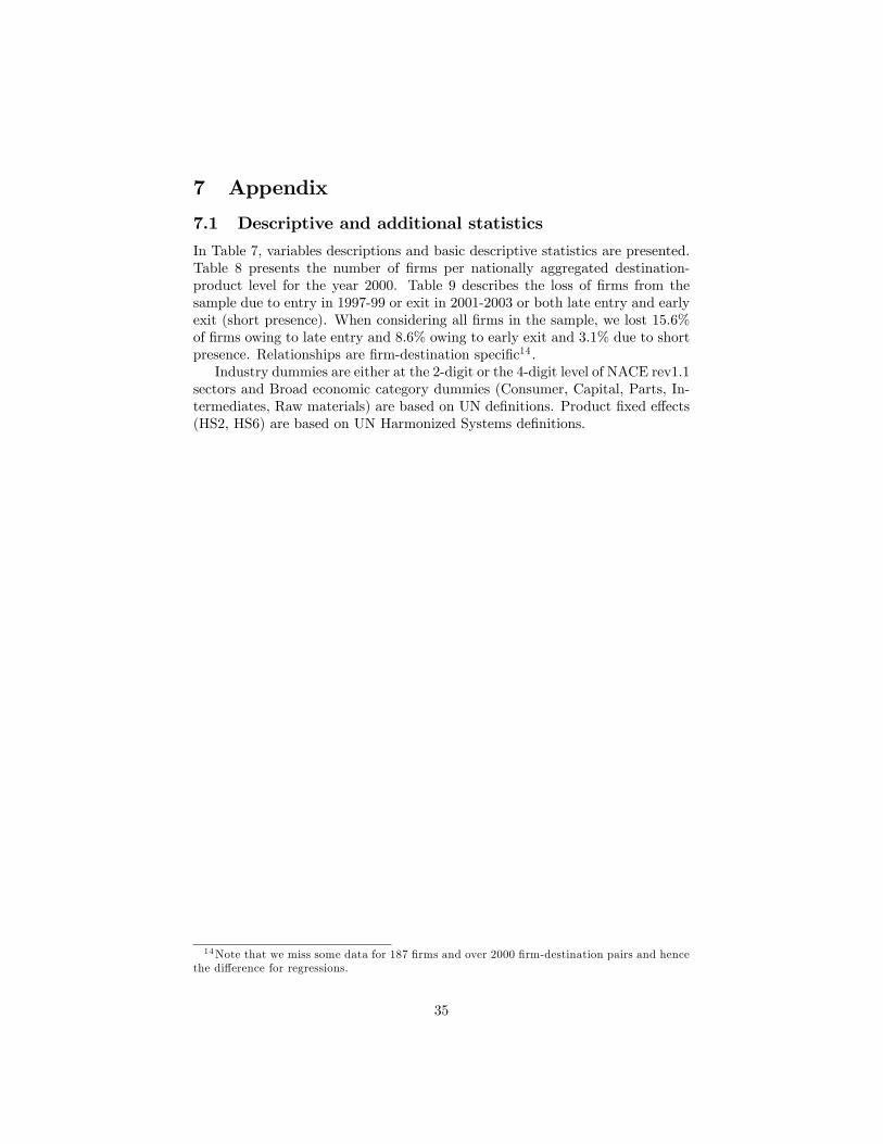
7 Appendix

7.1 Descriptive and additional statistics

In Table 7, variables descriptions and basic descriptive statistics are presented.Table 8 presents the number of firms per nationally aggregated destination-product level for the year 2000. Table 9 describes the loss of firms from thesample due to entry in 1997-99 or exit in 2001-2003 or both late entry and earlyexit (short presence). When considering all firms in the sample, we lost 15.6%of firms owing to late entry and 8.6% owing to early exit and 3.1% due to shortpresence. Relationships are firm-destination specific14 .Industry dummies are either at the 2-digit or the 4-digit level of NACE rev1.1

sectors and Broad economic category dummies (Consumer, Capital, Parts, In-termediates, Raw materials) are based on UN definitions. Product fixed effects(HS2, HS6) are based on UN Harmonized Systems definitions.

14Note that we miss some data for 187 firms and over 2000 firm-destination pairs and hencethe difference for regressions.

35

At the firm levelVariable Description N. Obs Mean SDFirm-destination levelTFP Total Factor Productivity is measured by

a modified Olley and Pakes (1996) definedin Altomonte and Békés (2010)

4405 0.589 1.051

Number ofemployees

Number of employees comes from the bal-ance sheet, includes all full time employees,and is in logs

4454 103.2 402.3

Export tosales

Export to total sales share is defined bybalance sheet of the firm.

4540 0.409 0.382

Multiproductd

Multiproduct dummy equals to 1 if thefirm sells more than one HS6 product tothe same country.

4540 0.950 0.220

Multi-destinationd

Multi-destination dummy equals to 1 if thefirm sells the same product to more thanone country

4540 0.824 0.381

Foreign d Foreign ownership is defined by adummy=1 if non-domestic residents holdmore than 10% of equity.

4540 0.400 0.490

Solvency Ra-tio

The Solvency Ratio (SR) is the ratio of netassets of the firm (equity, reserves, profits)plus long-term debts to total assets plusleftover stock (intermediate inputs and un-sold final output). It is defined in relativeterms to industry median.

4471 -0.078 0.541

Firm-destination levelLn Distance Distance (CEPII) 17084 6.907 1.003Ln GDP GDP (overall) 17084 19.522 1.604LnGDP/capita

GDP/capita 17084 9.616 0.756

Firm-product-destination levelRauch hetero-geneity

Rauch index of heterogeneity (dummy, 1 ifheterogeneous products, 0 for wholesale orreference priced), conservative measure isused. See Rauch (1999)

66911 0.888 0.315

Same prod,other count

Firm exports the same product to differentcountry (dummy)

66911 0.542 0.498

Same count,other prod

Firm exports other products to the samecountry (dummy)

66911 0.878 0.327

Large item d Large items are defined as products whoseunit value is above 90% of product rangeaverage. Unit values are defined as USDvolume over units given for the actual HS6product category.

66911 0.020 0.140

Asset d Assets are exported capital goods, when 66911 0.037 0.188Inventory d Inventories are exported intermediate

goods, when the profile of the firm is notthe production of such goods. Thesearelikely to have been inventories such asparts, raw materials.

66911 0.085 0.279

Table 7: Variables - descriptive stats

36

No of firms/cell No. Cells Percent1 15938 25.1%2 8982 14.1%3 6276 9.9%4 4432 6.9%5 3275 5.1%6 2616 4.1%7 2499 3.9%8 1600 2.5%9 1746 2.7%10 1530 2.4%More 14483 22.8%

Table 8: Number of observations

Firms RelationshipsLate entry 939 2633Early exit 518 2023

Short presence 184 393Not in sample 1641 5049In sample 4540 19754Total 6187 24803

Table 9: Share of temporary trade by good categories

37

(1) (2) (3) (4)Model Probit Probit Probit Lin.probTFP 0.064*** 0.015*** 0.019*** 0.016**

(0.007) (0.004) (0.004) (0.006)Export share in sales 0.211*** 0.216*** 0.236***

(0.013) (0.014) (0.014)N. of employees (log) 0.033*** 0.037*** 0.039***

(0.003) (0.003) (0.003)Multi-product firms (Dummy) 0.194*** 0.206*** 0.341***

(0.033) (0.036) (0.032)Solvency Ratio 0.013 0.019*** 0.020** 0.039***

(0.011) (0.007) (0.008) (0.013)Foreign-owned (Dummy) 0.024*** 0.026*** 0.013

(0.008) (0.008) (0.010)Sector dummies Nace2 Nace2 Nace4 Nace2Observations 4 353 4 335 3 986 4 335(Pseudo) R-squared 0.0926 0.312 0.340 0.237Log-likelihood -1670 -1255 -1162Robust standard errors in parentheses

*** p<0.01, ** p<0.05, * p<0.1

Table 10: Linear Probability and Probit models, dependent variable: T=1 iffirm is permanent trader, 0 if temporary

7.2 Firm level results

The model introduced in section 3.2 can be simplified by assuming that there isonly one market and there are no destination specific shocks. Thus, firms maybe permanent or temporary exporters as such. We have seen that even at thisaggregated level, there is quite some variation.We estimate firm i export status:

Pr(Ti) = F (α+ β′Fi + µi + εi) (10)

where Fi refers to firm level characteristics (ability, capital cost) and µi areindustry dummies, respectively. Our left hand side variable Ti = 1 if a firm ispermanent exporter, and Ti = 0 if temporary exporter.To measure the effect of firm level variables, we both use probit and linear

probability models, only to see very little difference. Firm level results confirmthat the key question is the impact of firm ability and cost of capital: Firmsare more likely to be permanent traders when more productive and have lowercapital cost.

38

nace Industry Sh. of perm.trade15 Food, beverages & tobacco 34%17 Textiles 44%18 Wearing apparel; fur 44%19 Leather, footwear 42%20 Wood and wood products 42%21 Pulp, paper and paper products 35%22 Publishing, printing 35%24 Chemicals and chemical products 55%25 Rubber and plastic products 47%26 Other non-metallic mineral products 50%27 Basic metals 52%28 Fabricated metal products, exc. machinery 38%29 Machinery and equipment 37%30 Offi ce machinery and computers 32%31 Electrical machinery and apparatus 47%32 Radio, television and comm. equipment 36%33 Medical, precision and optical instruments 45%34 Motor vehicles, trailers and semi-trailers 45%35 Other transport equipment 25%36 Furniture; manufacturing n.e.c. 44%

Table 11: Share of temporary trade by industries, firm-destination-product

7.3 Robustness test

We have carried out several robustness tests to the baseline results presented insection 4.2. After repeating the baseline specification (Base), we first presentthe possible impact of nuisance items, as we omitted small shipments worth lessthan 10.000USD (labelled as Non_small). This has somewhat reduced the sizeof coeffi cients but has not qualitatively affected results. Second, we dropped "ex-otic" destinations, keeping the 100 most important markets only (Top100 ).Theresults are basically unchanged from the baseline model, suggesting that it isnot far-away, peculiar locations that drive results.Third, we divided our sample into exports by single (SProd) and multi-

product (MProd) firms. There is a fairly small number of relationships of single-product firms at this level of aggregation. While firm level variables show limitedvariation, GDP and distance matters even within single product firms.

39

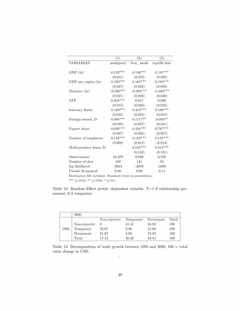
(1) (2) (3)VARIABLES multiprod Non_small top100 dest

GDP (ln) 0.133*** 0.156*** 0.131***(0.015) (0.019) (0.029)

GDP per capita (ln) 0.100*** 0.165*** 0.184***(0.027) (0.033) (0.058)

Distance (ln) -0.336*** -0.394*** -0.363***(0.021) (0.026) (0.040)

TFP 0.054*** 0.017 0.036(0.013) (0.020) (0.022)

Solvency Ratio 0.188*** 0.314*** 0.186***(0.035) (0.053) (0.055)

Foreign-owned, D 0.088*** 0.111*** 0.094**(0.025) (0.037) (0.041)

Export share 0.638*** 0.494*** 0.787***(0.037) (0.056) (0.057)

Number of employees 0.133*** 0.134*** 0.155***(0.008) (0.012) (0.013)

Multi-product firms, D 0.545*** 0.814***(0.142) (0.131)

Observations 16,379 9,899 6,750Number of dest 169 145 50log likelihood -9024 -3959 -3395Pseudo R-squared 0,08 0,08 0,11Destination RE included. Standard errors in parentheses,

*** p<0.01, ** p<0.05, * p<0.1

Table 12: Random Effect probit, dependent variable: T=1 if relationship per-manent, 0 if temporary

2000Non-exporter Temporary Permanent Total

Non-exporter 0 41.41 58.59 1001995 Temporary 76.07 8.86 15.00 100

Permanent 21.07 2.99 75.94 100Total 17.13 26.36 56.51 100

Table 13: Decomposition of trade growth between 1995 and 2000, 100 = totalvalue change in USD.

.

40

2000Non-exporter Temporary Permanent

Non-exporter 2.78 79.851995 Temporary -1.37 0.06 1.06

Permanent -4.60 -0.17 22.39

Table 14: Contributions to trade growth volume (1995 -2000), firm-destinationlevel

41