Misspecification Testing in a Class of

Conditional Distributional Models

Christoph Rothe and Dominik Wied∗

Columbia University and TU Dortmund

This Version: September 28, 2012

Abstract

We propose a specification test for a wide range of parametric models for the

conditional distribution function of an outcome variable given a vector of covari-

ates. The test is based on the Cramer-von Mises distance between an unrestricted

estimate of the joint distribution function of the data, and a restricted estimate

that imposes the structure implied by the model. The procedure is straightforward

to implement, is consistent against fixed alternatives, has non-trivial power against

local deviations of order n−1/2 from the null hypothesis, and does not require the

choice of smoothing parameters. In an empirical application, we use our test to

study the validity of various models for the conditional distribution of wages in the

US.

Keywords: Cramer-von Mises Distance, Quantile Regression, Distributional Regres-

sion, Location-Scale Model, Bootstrap, Wage Distribution

∗Christoph Rothe, Columbia University, Department of Economics, 420 W 118th St, New York, NY10027, USA. Email: cr2690@columbia.edu. Dominik Wied, TU Dortmund, Fakultat Statistik, CDI-Gebaude, D-44221 Dortmund, Germany. Email: wied@statistik.tu-dortmund.de. We would like tothank the associate editor, the referees, Roger Koenker and Blaise Melly for helpful comments. Financialsupport by Deutsche Forschungsgemeinschaft (SFB 823, project A1) is gratefully acknowledged.

1

1. Introduction

In this paper, we propose a general principle to construct omnibus specification test for

a wide range of parametric models for a conditional distribution function. For Y ∈ R an

outcome variable and X ∈ RK a vector of covariates, our interest is in testing the validity

of a model that asserts that there exists a possibly function-valued parameter θ such that

Pr(Y ≤ y|X = x) = F (y|x, θ) for all (y, x) ∈ Z, (1.1)

where F (·|·, θ) is a known function and Z denotes the support of Z = (Y,X). We refer

to any such specification as a conditional distributional model (CDM). The alternative

hypothesis is that equation (1.1) is violated for at least one value (y, x) ∈ Z. Allowing

unknown parameters to be function-valued is important in this setting, and constitutes

one of the main innovations of our approach. We also discuss an extension of our proce-

dure that allows to test the hypothesis in (1.1) for all (y, x) in some set S ⊂ Z chosen by

the analyst. Through an appropriate choice of S, one can test whether the parametric

model provides an adequate fit over a particular range of the conditional distribution

function, such as e.g. the area below or above the conditional median.

Our general setting covers a wide range of CDMs that are of great importance in

empirical applications. The leading example is certainly the linear quantile regression

model (Koenker and Bassett, 1978; Koenker, 2005), which implies a linear structure for

the inverse of the conditional CDF, namely that F−1(τ |x, θ) = x′θ(τ) for some functional

parameter θ(·) that is strictly increasing in each of its components. Nonlinear versions of

quantile regression could be considered as well. Another example is the linear location-

scale shift model (Koenker and Xiao, 2002), under which F−1(τ |x, θ) = x′β + x′γQϵ(τ),

with Qϵ a univariate quantile function and θ(·) = (β, γ,Qϵ(·)). Our setting also covers

the distributional regression model (Foresi and Peracchi, 1995), where the conditional

CDF is modeled by a series of binary response models with varying “cutoffs”. That is,

the conditional CDF is specified as F (y|x, θ) = Λ (x′θ(y)) , where Λ is a known strictly

2

increasing link function such as e.g. the logistic or standard normal distribution function,

and θ(·) is again a function-valued parameter. This class of models has recently received

considerable attention in the econometrics literature (e.g. Chernozhukov et al., 2009;

Koenker, 2010; Fortin et al., 2011; Rothe, 2011).

Our test is an extension of the method proposed by Andrews (1997) in the context

of parametric models indexed by finite dimensional parameters. The basic idea is to

compare an unrestricted estimate of the joint distribution function of Y and X to a

restricted estimate that imposes the structure implied by the CDM. For example, to test

the validity of the linear quantile regression model we would first obtain an estimate

of the conditional CDF of Y given X by inverting the estimated conditional quantile

function, and then transform this object into an estimate of the joint CDF of (Y,X)

by “integrating up” the conditioning argument. This restricted CDF estimate can then

be compared to the joint empirical distribution function of the data, which is the most

natural unrestricted estimate.

Our test statistic is a Cramer-von Mises type measure of distance between the two

above-mentioned objects, and is therefore called a Generalized Conditional Cramer-von

Mises (GCCM) test. We reject the null hypothesis that the parametric model is correctly

specified whenever this distance is “too large”. Since our test statistic is not asymptoti-

cally pivotal, critical values cannot be tabulated, but can be obtained via the bootstrap.

While our test is thus computationally somewhat involved, it is straightforward to im-

plement and has a number of attractive theoretical properties: It is consistent against all

fixed alternatives, has non-trivial power against local deviations from the null hypothe-

sis of order n−1/2 (where n denotes the sample size), and does not require the choice of

smoothing parameters.

The correct specification of CDMs of the type considered in this paper is critical

in many areas of applied statistics. In economics, for example, such specifications are

employed extensively to study differentials in the distribution of wages between two

time periods, or two subgroups of a particular population (see e.g. Machado and Mata,

3

2005,Chernozhukov et al., 2009 or Rothe, 2011). From a statistical point of view, these

methods first obtain an estimate of the conditional CDF of Y given X. In a second step,

this function is integrated over the conditioning argument with respect to another CDF,

whose exact form depends on the particular application, yielding a new univariate dis-

tribution function. As a final step, features of this new distribution function, such as its

mean or quantiles, are computed. Our concern is the implementation of the first step of

this procedure. For example, the Machado and Mata (2005) decomposition relies on the

assumption that the entire conditional distribution of wages given observable individual

characteristics can be described by a linear quantile regression model. If this assump-

tion is violated, the method can potentially lead to inappropriate conclusions (see Rothe,

2010, for some simulation evidence). From a practitioner’s point of view, misspecification

is a serious concern in this context, as the conditional quantiles of the wage distribution

are e.g. known to be extremely flat in the vicinity of the legal minimum wage, and might

thus not be described adequately by a linear specification in this region (Chernozhukov

et al., 2009). Our testing procedure can be used to formally investigate this issue.

As an additional contribution, our paper provides some empirical evidence on the

last point: using US data from the Current Population Survey, we show that typical

specifications of linear location-scale models and linear quantile regressions containing

a rich set of covariates are frequently rejected by our GCCM test even for small and

moderate sample sizes. On the other hand, we find that the distributional regression

model, which has thus far received only limited interest in the literature, typically cannot

be rejected in such settings.

There exists an extensive literature on specification testing in parametric models for

the conditional expectation function (see e.g. Bierens, 1990, Hardle and Mammen, 1993,

Bierens and Ploberger, 1997, Stute, 1997 and Horowitz and Spokoiny, 2001), and for

the conditional quantile function at one particular quantile, such as the median (see

e.g. Zheng, 1998, Bierens and Ginther, 2001, Horowitz and Spokoiny, 2002, He and Zhu,

2003, and Whang, 2006). In comparison, the related problem of testing the validity

4

of a model for the entire conditional distribution function that we study in this paper

has received much less attention. Andrews (1997) proposes a test for CDMs indexed

by finite-dimensional parameters. Koenker and Machado (1999) and Koenker and Xiao

(2002) consider specification testing in a quantile regression context, and propose tests for

e.g. the validity of the location-scale model, but not the validity of the quantile regression

model itself. Galvao et al. (2011) test for threshold effects in linear quantile regression in a

time series context. Escanciano and Velasco (2010) and Escanciano and Goh (2010) both

propose testing procedures for the null hypothesis that a conditional quantile restriction

is valid over a range of quantiles in different settings, that both include the usual quantile

regression model with independent observations as a special case. We are not aware of

any paper that provides a general approach to testing the validity of CDMs indexed by

possibly function-valued parameters.

2. Testing General Conditional Distributional Models

2.1. Testing Problem. We observe an outcome variable Yi ∈ R and a vector of

explanatory variables Xi ∈ RK for i = 1, . . . , n. The cumulative distribution function

(CDF) of Zi = (Yi, Xi) and Xi are denoted by H and G, respectively. We assume

throughout the paper that the data points are independent and identically distributed.

Our aim is to test the validity of certain classes of parametric specifications for the

conditional CDF F of Yi given Xi. Let F be the class of all conditional distribution

functions on the support of Y given X that satisfy certain weak regularity conditions

given below, and consider a CDM

F0 = {F (·|·, θ) for some θ ∈ B(U ,Θ)} ⊂ F ,

i.e. a family of conditional distribution functions indexed by a (potentially) functional

parameter θ taking values in B(U ,Θ), the class of mappings u 7→ θ(u) such that θ(u) ∈

Θ ⊂ Rp for u ∈ U ⊂ R. The hypothesis that we want to test is that F coincides with an

5

element of F0:

H0 : F (y|x) = F (y|x, θ) for some θ ∈ B(U ,Θ) and all (y, x) ∈ Z (2.1)

vs. H1 : F (y|x) = F (y|x, θ) for all θ ∈ B(U ,Θ) and some (y, x) ∈ Z. (2.2)

This paper proposes a testing procedure of the problem in (2.1)–(2.2) for CDMs in

which the true value of the functional parameter is identified under the null hypothesis

through a moment condition. Specifically, let ψ : Z × Θ × U 7→ Rp be a uniformly

integrable function whose exact form depends on F0, and suppose that for every u ∈ U

the equation

Ψ(θ, u) := E (ψ(Z, θ, u)) = 0 (2.3)

has a unique solution θ0(u). We assume that under the null hypothesis any value

θ ∈ B(U ,Θ) of the functional parameter that satisfies F (y|x) = F (y|x, θ) for all (y, x) ∈ Z

also satisfies θ(u) = θ0(u) for all u ∈ U . The moment condition (2.3) thus uniquely de-

termines the value of the “true” functional parameter. Under the alternative, θ0 remains

well-defined as the solution to (2.3), and can thus be thought of as a pseudo-true value

of the functional parameter in this case. General results on estimation and inference in

this class of models are derived in Chernozhukov et al. (2009). We discuss in Section 4

how a large class of empirically relevant specifications fits into this framework.

2.2. Test Statistic. To motivate a test statistic for the problem in (2.1)–(2.2), note

that, following the above discussion, our null hypothesis can be equivalently stated as

F (y|x) = F (y|x, θ0) for all (y, x) ∈ RK+1, (2.4)

with θ0(u) the unique solution to (2.3). This holds because F (·|·, θ0) is the only element

of F0 that is a potential candidate value for the true conditional CDF F of Yi given

6

Xi by assumption. Since F (y|x) = E(I{Y ≤ y}|X = x), where I{a ≤ b} denotes the

indicator for the event that each component of a is weakly smaller than the corresponding

component of b, equation (2.4) is a restriction on the conditional moments of Y given

X, that can be transformed into a restriction on unconditional moments without loss

of information by “integrating up” with respect to the marginal distribution G of the

conditioning variable X. Writing

H(y, x) =

∫F (y|t)I{t ≤ x}dG(t) and H0(y, x) =

∫F (y|t, θ0)I{t ≤ x}dG(t)

for the joint CDF of (Y,X) and another CDF that imposes the structure implied by the

CDM, respectively, it follows from Billingsley (1995, Theorem 16.10(iii)) that our testing

problem (2.1)–(2.2) can be restated as

H0 : H(y, x) = H0(y, x) for all (y, x) ∈ RK+1

vs. H1 : H(y, x) = H0(y, x) for some (y, x) ∈ RK+1.

Of course, the idea to transform conditional moment restrictions into unconditional ones

is not new in the literature on specification testing. It is used for example by Stute (1997)

in the context of testing parametric specifications of conditional expectation functions.

Given the above representation of the testing problem, we propose to construct a

specification test for the CDM F0 based on a Cramer-von Mises type measure of distance

between estimates H and H0, scaled by the sample size. Specifically, the test statistic Tn

is defined as

Tn = n

∫(Hn(y, x)− H0

n(y, x))2dHn(y, x) =

n∑i=1

(Hn(Yi, Xi)− H0n(Yi, Xi))

2,

7

where

Hn(y, x) = n−1

n∑i=1

I{Yi ≤ y}I{Xi ≤ x} and

H0n(y, x) = n−1

n∑i=1

Fn(y|Xi)I{Xi ≤ x},

with Fn(y|x) = F (y|x, θn) a parametric estimate of F based on an estimate θn of θ0. Here

we take θn to be an approximate Z-estimator satisfying

∥Ψn(θn(u), u)∥ = infθ∈Θ

∥Ψn(θ, u)∥+ ηn (2.5)

for some (possibly random) variable ηn = op(n−1/2) and every u ∈ U . The function

Ψn(θ, u) := n−1∑n

i=1 ψ(Zi, θ, u) is the sample analogue of the moment condition in (2.3).

This approach is feasible for all examples we consider in this paper.

Under general conditions described in the following section, the random process

(y, x) 7→ Hn(y, x) − H0n(y, x) converges to zero in probability under the null hypothe-

sis, and to a non-zero probability limit under the alternative. Large realizations of Tn

thus indicate a possible violation of the null. Since our testing principle shares some

similarities with the Conditional Kolmogorov test in Andrews (1997), we refer to our test

in the following as a Generalized Conditional Cramer-von Mises (GCCM) test. The rea-

son for departing from Andrews (1997) with respect to the distance measure is that our

simulation experiments suggested that Cramer-von Mises type statistics have somewhat

better power properties than those based on the Kolmogorov distance.

2.3. Bootstrap Critical Values. As we show in more detail below, for most common

CDMs the asymptotic null distribution of Tn is non-pivotal and depends on the data

generating process in a complex fashion. We therefore propose to obtain critical values for

our test via a semiparametric bootstrap procedure. Such a procedure is computationally

expensive but convenient from a practical point of view, since it avoids the complicated

8

problem of estimating null distribution of Tn directly. While the approach cannot be

expected to yield any higher-order improvements over a standard large sample test, one

could of course always improve the level accuracy by using a form of the iterated bootstrap

(see e.g. Hall, 1986 or Beran, 1988).

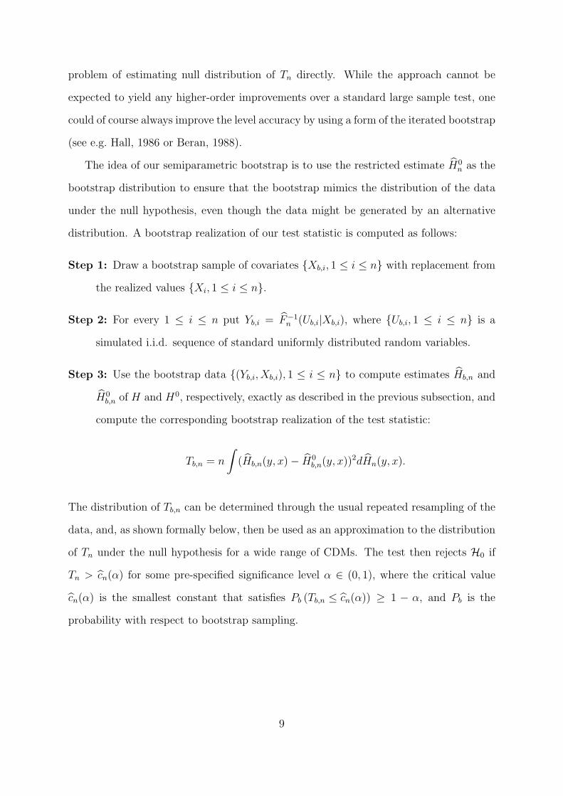
The idea of our semiparametric bootstrap is to use the restricted estimate H0n as the

bootstrap distribution to ensure that the bootstrap mimics the distribution of the data

under the null hypothesis, even though the data might be generated by an alternative

distribution. A bootstrap realization of our test statistic is computed as follows:

Step 1: Draw a bootstrap sample of covariates {Xb,i, 1 ≤ i ≤ n} with replacement from

the realized values {Xi, 1 ≤ i ≤ n}.

Step 2: For every 1 ≤ i ≤ n put Yb,i = F−1n (Ub,i|Xb,i), where {Ub,i, 1 ≤ i ≤ n} is a

simulated i.i.d. sequence of standard uniformly distributed random variables.

Step 3: Use the bootstrap data {(Yb,i, Xb,i), 1 ≤ i ≤ n} to compute estimates Hb,n and

H0b,n of H and H0, respectively, exactly as described in the previous subsection, and

compute the corresponding bootstrap realization of the test statistic:

Tb,n = n

∫(Hb,n(y, x)− H0

b,n(y, x))2dHn(y, x).

The distribution of Tb,n can be determined through the usual repeated resampling of the

data, and, as shown formally below, then be used as an approximation to the distribution

of Tn under the null hypothesis for a wide range of CDMs. The test then rejects H0 if

Tn > cn(α) for some pre-specified significance level α ∈ (0, 1), where the critical value

cn(α) is the smallest constant that satisfies Pb (Tb,n ≤ cn(α)) ≥ 1 − α, and Pb is the

probability with respect to bootstrap sampling.

9

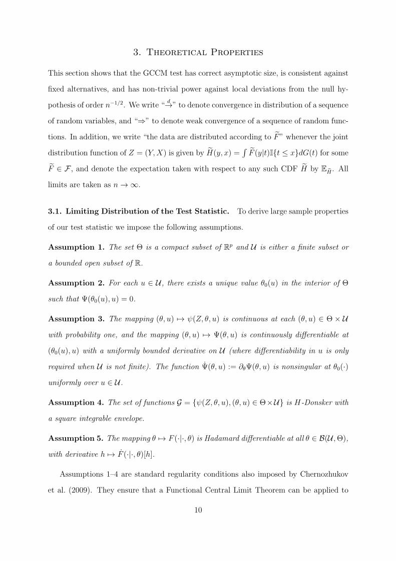
3. Theoretical Properties

This section shows that the GCCM test has correct asymptotic size, is consistent against

fixed alternatives, and has non-trivial power against local deviations from the null hy-

pothesis of order n−1/2. We write “d→” to denote convergence in distribution of a sequence

of random variables, and “⇒” to denote weak convergence of a sequence of random func-

tions. In addition, we write “the data are distributed according to F” whenever the joint

distribution function of Z = (Y,X) is given by H(y, x) =∫F (y|t)I{t ≤ x}dG(t) for some

F ∈ F , and denote the expectation taken with respect to any such CDF H by EH . All

limits are taken as n→ ∞.

3.1. Limiting Distribution of the Test Statistic. To derive large sample properties

of our test statistic we impose the following assumptions.

Assumption 1. The set Θ is a compact subset of Rp and U is either a finite subset or

a bounded open subset of R.

Assumption 2. For each u ∈ U , there exists a unique value θ0(u) in the interior of Θ

such that Ψ(θ0(u), u) = 0.

Assumption 3. The mapping (θ, u) 7→ ψ(Z, θ, u) is continuous at each (θ, u) ∈ Θ × U

with probability one, and the mapping (θ, u) 7→ Ψ(θ, u) is continuously differentiable at

(θ0(u), u) with a uniformly bounded derivative on U (where differentiability in u is only

required when U is not finite). The function Ψ(θ, u) := ∂θΨ(θ, u) is nonsingular at θ0(·)

uniformly over u ∈ U .

Assumption 4. The set of functions G = {ψ(Z, θ, u), (θ, u) ∈ Θ×U} is H-Donsker with

a square integrable envelope.

Assumption 5. The mapping θ 7→ F (·|·, θ) is Hadamard differentiable at all θ ∈ B(U ,Θ),

with derivative h 7→ F (·|·, θ)[h].

Assumptions 1–4 are standard regularity conditions also imposed by Chernozhukov

et al. (2009). They ensure that a Functional Central Limit Theorem can be applied to

10

the Z-estimator process u 7→√n(θn(u)−θ0(u)). Assumption 5 is a smoothness condition

that can be verified directly in applications. Together with the Functional Delta Method,

it implies that the restricted CDF estimator process (y, x) 7→√n(H0

n(y, x) − H0(y, x))

also converges to a Gaussian limit process G2. This convergence can be shown to be

jointly with that of the empirical CDF process (y, x) 7→√n(Hn(y, x)−H(y, x)) to an H-

Brownian Bridge G1. The limiting distribution of our test statistic Tn then follows from

an application of the continuous mapping theorem, and from the fact that the functions

H and H0 coincide under the null hypothesis, but differ on a set with positive probability

under the alternative.

Theorem 1. Under Assumption 1–5, the following statements hold.

i) Under the null hypothesis, i.e. when the data are distributed according to some F

that satisfies (2.1),

Tnd→∫

(G1(y, x)−G2(y, x))2 dH(y, x),

where G = (G1,G2) is a bivariate mean zero Gaussian process given in the Appendix.

ii) Under any fixed alternative, i.e. when the data are distributed according to some F

that satisfies (2.2),

limn→∞

P (Tn > c) → 1 for all constants c > 0.

3.2. Local Alternatives. This section derives the limiting distribution of our test

statistic under a sequence of local alternatives that shrink towards an element of F0 at

rate n−1/2, where n denotes the sample size. That is, the conditional distribution function

of Y given X is given by

Qn(y|x) = (1− δ/√n)F ∗(y|x) + (δ/

√n)Q(y|x), (3.1)

11

where F ∗ is a CDF such that F ∗(y|x) = F (y|x, θ) for some θ ∈ B(U ,Θ) and all (y, x) ∈ Z,

Q is a CDF such that Q(y|x) = F (y|x, θ) for all θ ∈ B(U ,Θ) and some (y, x) ∈ Z, and

δ ≤ n1/2 is some constant, satisfying the following assumption.

Assumption 6. The sequence Hn(y, x) =∫Qn(y|t)I{t ≤ x}dG(t) of distribution func-

tions implied by the local alternative Qn given in (3.1) is contiguous to the distribution

function H∗(y, x) =∫F ∗(y|t)I{t ≤ x}dG(t) implied by F ∗.

The requirement that the local alternatives are contiguous to the limiting distribution

function is standard when analyzing local power properties. When the conditional distri-

bution functions F ∗ and Q admit conditional density functions f ∗ and q with respect to

the same σ-finite measure (e.g. the Lebesgue measure), respectively, a sufficient condition

for contiguity is that sup{(x,y):f∗(y|x)>0} q(y|x)/f ∗(y|x) <∞. Intuitively, this would be the

case when Q has lighter tails than F ∗. See Rothe and Wied (2012) for a formal proof.

The following theorem shows that under local alternatives of the form (3.1) the

limiting distribution of Tn contains an additional deterministic shift function ensur-

ing non-trivial local power of the test. To describe this function, define ΨQ(θ, u) =

EQ (ψ(Z, θ, u)) and Ψ∗(θ, u) = EF ∗ (ψ(Z, θ, u)), and let θQ and θ∗ be the functions satis-

fying ΨQ(θQ(u), u) = 0 and Ψ∗(θ∗(u), u) = 0 for all u ∈ U , respectively.

Theorem 2. Under Assumption 1–6, and if the data are distributed according to a local

alternative Qn as given in (3.1),

Tnd→∫

(G1(y, x)−G2(y, x) + µ(y, x))2 dH(y, x).

where µ(y, x) = δ∫(Q(y|t) − F (y|t, θ∗) + F (y|t, θ∗)[h])I{t ≤ x}dG(t) and the function h

is given by h(u) = ∂θ′ΨF ∗(θ∗(u), u)−1ΨQ(θ∗(u), u).

Note that the function F ∗ to which the local alternative Qn shrinks can be chosen

as F (·|·, θQ), the probability limit of the estimator Fn under Q. In this case, we have

12

ΨQ(θ∗(u), u) = 0 for all u ∈ U , and hence the drift term in Theorem 2 simplifies to

µ(y, x) = δ

∫(Q(y|t)− F (y|t, θ∗)) I{t ≤ x}dG(t),

which is proportional to the difference between the joint CDFs implied by Q and F ∗.

3.3. Validity of the Bootstrap. As a final step, we establish asymptotic validity of

the critical values obtained via the bootstrap procedure described in Section 2.3. This

does not require any further assumptions. Under the null hypothesis, Assumptions 1–

5 ensure that the bootstrap consistently estimates the limiting distribution of the test

statistic Tn, and hence consistently estimates the true critical values. Under any fixed

alternative, the bootstrap critical values can be shown to be bounded in probability.

Together with Theorem 1(ii), this implies that our test is consistent. Finally, since

contiguity preserves convergence in probability, it follows from Assumption 6 that under

any local alternative the bootstrap critical values converge to the same value as under

the null hypothesis. We can thus deduce from Anderson’s Lemma that our test has

non-trivial local power. The following theorem formalizes these arguments.

Theorem 3. Under Assumption 1–6, the following statements hold for any α ∈ (0, 1):

i) Under the null hypothesis, i.e. when the data are distributed according to some CDF

F that satisfies (2.1), we have that

limn→∞

P (Tn > cn(α)) = α.

ii) Under any fixed alternative, i.e. when the data are distributed according to some CDF

F that satisfies (2.2), we have that

limn→∞

P (Tn > cn(α)) = 1.

iii) Under any local alternative, i.e. when the data are distributed according to some

13

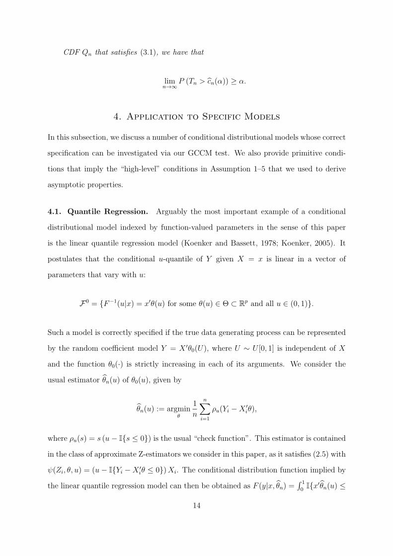
CDF Qn that satisfies (3.1), we have that

limn→∞

P (Tn > cn(α)) ≥ α.

4. Application to Specific Models

In this subsection, we discuss a number of conditional distributional models whose correct

specification can be investigated via our GCCM test. We also provide primitive condi-

tions that imply the “high-level” conditions in Assumption 1–5 that we used to derive

asymptotic properties.

4.1. Quantile Regression. Arguably the most important example of a conditional

distributional model indexed by function-valued parameters in the sense of this paper

is the linear quantile regression model (Koenker and Bassett, 1978; Koenker, 2005). It

postulates that the conditional u-quantile of Y given X = x is linear in a vector of

parameters that vary with u:

F0 = {F−1(u|x) = x′θ(u) for some θ(u) ∈ Θ ⊂ Rp and all u ∈ (0, 1)}.

Such a model is correctly specified if the true data generating process can be represented

by the random coefficient model Y = X ′θ0(U), where U ∼ U [0, 1] is independent of X

and the function θ0(·) is strictly increasing in each of its arguments. We consider the

usual estimator θn(u) of θ0(u), given by

θn(u) := argminθ

1

n

n∑i=1

ρu(Yi −X ′iθ),

where ρu(s) = s (u− I{s ≤ 0}) is the usual “check function”. This estimator is contained

in the class of approximate Z-estimators we consider in this paper, as it satisfies (2.5) with

ψ(Zi, θ, u) = (u− I{Yi −X ′iθ ≤ 0})Xi. The conditional distribution function implied by

the linear quantile regression model can then be obtained as F (y|x, θn) =∫ 1

0I{x′θn(u) ≤

14

y}du. Note that F (y|x, θn) is monotone in y by construction for every x, even if the

estimated quantile curve u 7→ x′θn(u) is not. The test statistic Tn can then be computed

in a straightforward fashion. Our asymptotic analysis in Section 3 applies to the linear

quantile regression example under the conditions of the following theorem.

Theorem 4. Suppose that (i) the distribution function F (·|X) admits a density function

f(·|X) that is continuous, bounded and bounded away from zero at X ′θ0(u), uniformly

over u ∈ U = (0, 1), almost surely. (ii) The matrix E(XX ′) is finite and of full rank,

(iii) the parameter θ0(·) solving E (ψ (Z, θ0(u), u)) = 0 is such that θ0(u) is in the interior

of the parameter space Θ for every u ∈ (0, 1). Then Assumption 1–5 hold for the linear

quantile regression model with F (y|x, θ)[h(·)] = −f(y|x)x′ [h (F (y|x, θ))].

The role of the conditions in Theorem 4, which are standard in the literature, is

essentially ensure that the moment condition E (ψ (Z, θ0(u), u)) = 0 has a unique solution

θ0(u) for every u ∈ U , and that the process u 7→√n(θn(u)−θ0(u) converges to a Gaussian

limit under both the null hypothesis and the alternative. Note that our Theorem imposes

strong conditions on the distribution of Y given X in order to ensure that Assumption 1–

5 hold with U = (0, 1). If it is unreasonable to assume that f(·|X) is uniformly bounded

away from zero (e.g. because the support of Y is unbounded), one could still test the

validity of the linear quantile regression model for u ∈ (ϵ, 1− ϵ) for some ϵ > 0 by using

an extension of our test described in Section 5 below.

4.2. Location Shift and Location-Scale Shift Models. The testing procedures

proposed in this paper can also be used to assess the validity of various special cases of

quantile regression. A leading example is the linear location-scale shift model

F0 = {F−1(u|x) = x′β + x′γQϵ(u) for some

θ(u) = (β, γ,Qϵ(u)) ∈ R2p+1 and all u ∈ (0, 1)}, (4.1)

15

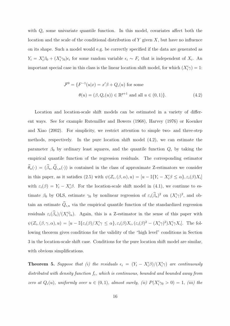
with Qϵ some univariate quantile function. In this model, covariates affect both the

location and the scale of the conditional distribution of Y given X, but have no influence

on its shape. Such a model would e.g. be correctly specified if the data are generated as

Yi = X ′iβ0 + (X ′

iγ0)ϵi for some random variable ϵi ∼ Fε that is independent of Xi. An

important special case in this class is the linear location shift model, for which (X ′iγ) = 1:

F0 = {F−1(u|x) = x′β +Qϵ(u) for some

θ(u) = (β,Qϵ(u)) ∈ Rp+1 and all u ∈ (0, 1)}. (4.2)

Location and location-scale shift models can be estimated in a variety of differ-

ent ways. See for example Rutemiller and Bowers (1968), Harvey (1976) or Koenker

and Xiao (2002). For simplicity, we restrict attention to simple two- and three-step

methods, respectively. In the pure location shift model (4.2), we can estimate the

parameter β0 by ordinary least squares, and the quantile function Qϵ by taking the

empirical quantile function of the regression residuals. The corresponding estimator

θn(·) = (βn, Qϵ,n(·)) is contained in the class of approximate Z-estimators we consider

in this paper, as it satisfies (2.5) with ψ(Zi, (β, α), u) = [u − I{Yi − X ′iβ ≤ α}, εi(β)Xi]

with εi(β) = Yi − X ′iβ. For the location-scale shift model in (4.1), we continue to es-

timate β0 by OLS, estimate γ0 by nonlinear regression of εi(βn)2 on (X ′

iγ)2, and ob-

tain an estimate Qϵ,n via the empirical quantile function of the standardized regression

residuals εi(βn)/(X′iγn). Again, this is a Z-estimator in the sense of this paper with

ψ(Zi, (β, γ, α), u) = [u − I{εi(β)/X ′iγ ≤ α}, εi(β)Xi, (εi(β)

2 − (X ′iγ)

2)X ′iγXi]. The fol-

lowing theorem gives conditions for the validity of the “high level” conditions in Section

3 in the location-scale shift case. Conditions for the pure location shift model are similar,

with obvious simplifications.

Theorem 5. Suppose that (i) the residuals ϵi = (Yi − X ′iβ)/(X

′iγ) are continuously

distributed with density function fϵ, which is continuous, bounded and bounded away from

zero at Qϵ(u), uniformly over u ∈ (0, 1), almost surely, (ii) P (X ′iγ0 > 0) = 1, (iii) the

16

matrix E(XX ′) is finite and of full rank, (iv) E(Y 2) is finite, and (v) the parameter θ0(·) =

(β0, γ0, Qϵ(·)) solving E (ψ (Z, θ0(u), u)) = 0 is such that θ0(u) is in the interior of the

parameter space Θ for every u ∈ (0, 1). Then Assumption 1–5 hold for the linear location-

scale shift model with F (y|x, θ)[h(·)] = −fϵ((y − x′β)/(x′γ))(x′β + x′γQϵ(h(F (y|x, θ)))).

4.3. Distributional Regression. Another class of CDMs covered by our framework

are so-called distributional regression models, which were introduced by Foresi and Per-

acchi (1995). These models have recently received considerable interest in the economics

literature, as they conveniently allow to model certain features of conditional wage distri-

butions, such as nonlinearities around the level of the minimum wage (e.g. Chernozhukov

et al., 2009; Rothe, 2011). The basic idea is to directly model the conditional CDF of

Y given X through a family of binary response models for the event that the dependent

variable Y exceeds some threshold y ∈ R. More specifically the model is given by

F0 = {F (y|x) = Λ(x′θ(y)) for some θ(y) ∈ Θ ⊂ Rp and all y ∈ R}, (4.3)

where Λ(·) is a known strictly increasing link function, e.g. the logistic or standard normal

distribution function, or simply the identity function. Distributional regression models

can differ substantially from a classical quantile regression model using the same set of

covariates, and no class of models is more general than the other. Both classes, however,

contain the location shift model as special case. See Koenker (2010) for some theoretical

comparisons of the two approaches in this context. An advantage of distributional regres-

sion relative to quantile regression is that it does not require the dependent variable to

be continuously distributed, which can be an important in certain empirical applications.

Since for every threshold value y ∈ R the distributional regression model resembles a

standard binary response model, it can be fitted the same way one would e.g. proceed with

a logistic regression. A natural estimator for the functional parameter θ0(·) is the “point-

wise” maximum likelihood estimator θn(·), which solves the equation ∥Ψn(θn(y), y)∥ =

0, with Ψn(θ, y) := n−1∑n

i=1 ψ(Zi, θ, y) and ψ(Zi, θ, y) = (Λ(X ′iθ) (1− Λ(X ′

iθ)))−1 ×

17

(Λ(X ′iθ)− I{Yi ≤ y})λ(X ′

iθ)Xi the usual score function, and λ the derivative of Λ. The

estimated conditional CDF of Y given X is then given by Fn(y|x) = Λ(x′θn(y)), and

the test statistic Tn is straightforward to compute from this expression. The following

theorem gives conditions for the distributional regression model to satisfy the “high level”

conditions in Section 3.

Theorem 6. Suppose that (i) the support Y of Y is either a finite set or a bounded open

subset of R, (ii) the distribution function F (·|X) admits a density function f(·|X) that is

continuous, bounded and bounded away from zero at all y ∈ Y, almost surely, (iii) the ma-

trix E(XX ′) is finite and of full rank, (iv) the parameter θ0(·) solving E (ψ (Z, θ0(y), y)) =

0 is such that θ0(y) is in the interior of the parameter space Θ for every y ∈ Y, and (v)

the quantity Λ(X ′θ) is bounded away from zero and one uniformly over θ ∈ Θ, almost

surely. Then Assumption 1–5 hold for the distributional regression model in (4.3) with

F (y|x, θ)[h(·)] = (∂Λ (x, θ(y)) /∂θ′)[h(y)].

5. Extension: Testing over a Subset of the Support

In some applications, it is not only interesting to test the validity of a CDM for the

entire conditional CDF, but also its adequacy over some range of the conditional distri-

bution. For example, for models formulated in terms of conditional quantiles, one might

be interested in whether the model is correctly specified for all conditional u-quantiles

with u ∈ (uL, uU) and 0 < uL < uU < 1. Another question that might be of interest is

whether the parametric model correctly describes the conditional CDF on the subset of

the support where Y and/or some components of X takes values in a particular interval.

To accommodate such settings, we can consider the following generalization of our testing

problem (2.1)–(2.2):

H0 : F (y|x) = F (y|x, θ) for some θ ∈ B(U ,Θ) and all (y, x) ∈ S (5.1)

vs. H1 : F (y|x) = F (y|x, θ) for all θ ∈ B(U ,Θ) and some (y, x) ∈ S (5.2)

18

for some suitably chosen closed and connected set S ⊂ Z. The two above-mentioned

examples correspond to choosing S = {(y, x) : F−1(uL|x) ≤ y ≤ F−1(uU |x)} for 0 < uL <

uU < 1, and S = {(y, x) : yL ≤ y ≤ yU , xL ≤ x ≤ xU} for some −∞ ≤ yL < yU ≤ ∞ and

−∞ ≤ xL < xU ≤ ∞, respectively. Of course, other choices of S are possible as well.

Our GCCM test can be adapted to the modified testing problem in (5.1)–(5.2) as

follows. First, it might be necessary to modify the function ψ such that θn remains

consistent for a population value θ0 satisfying F (y|x) = F (y|x, θ0) for all (y, x) ∈ S

under the null hypothesis. The details of this step critically depend on the type of CDM

under consideration, and also the exact form of the set S. It is therefore difficult to give

a general recipe. For example, when testing the linear quantile regression specification

and S = {(y, x) : y ≥ yL} for some constant yL ∈ R one could e.g. work with the

censored quantile regression estimator of Powell (1986). Second, one has to redefine the

test statistic such that the difference Hn(y, x)− H0n(y, x) is only evaluated over S. This

can be accomplished by simply putting

Tn = n

∫S

(Hn(y, x)− H0n(y, x))

2dHn(y, x) =n∑

i=1

I{(Yi, Xi) ∈ S}(Hn(y, x)− H0n(y, x))

2.

Third, one has to modify the bootstrap sampling scheme in order to impose the new null

hypothesis (5.1). To do so, one can obtain a bootstrap data set {(Yb,i, Xb,i), 1 ≤ i ≤ n}

by i.i.d. sampling from the CDF H∗n, where

H∗n(y, x) =

Hn(y, x) if (y, x) /∈ S

H0n(y, x) if (y, x) ∈ S,

and proceed as before with the new data set. Theoretical properties analogous to those

derived in Section 3 can be established for the modified testing procedure using the same

type of arguments. If the set S is unknown, it can be replaced in the steps outlined

above by some consistent estimate Sn. It can be shown that this does not affect the

test’s asymptotic properties as long as Sn satisfies the weak regularity condition that

19

n−1∑n

i=1(I{(Yi, Xi) ∈ Sn} − I{(Yi, Xi) ∈ S}) p→ 0.

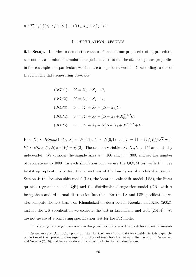
6. Simulation Results

6.1. Setup. In order to demonstrate the usefulness of our proposed testing procedure,

we conduct a number of simulation experiments to assess the size and power properties

in finite samples. In particular, we simulate a dependent variable Y according to one of

the following data generating processes:

(DGP1): Y = X1 +X2 + U,

(DGP2): Y = X1 +X2 + V,

(DGP3): Y = X1 +X2 + (.5 +X1)U,

(DGP4): Y = X1 +X2 + (.5 +X1 +X22 )

1/2U,

(DGP5): Y = X1 +X2 + .2(.5 +X1 +X22 )

3/2 + U.

Here X1 ∼ Binom(1, .5), X2 ∼ N(0, 1), U ∼ N(0, 1) and V = (1 − 2V ∗1 )V

∗2 /

√8 with

V ∗1 ∼ Binom(1, .5) and V ∗

2 = χ2(2). The random variables X1, X2, U and V are mutually

independet. We consider the sample sizes n = 100 and n = 300, and set the number

of replications to 1000. In each simulation run, we use the GCCM test with B = 199

bootstrap replications to test the correctness of the four types of models discussed in

Section 4: the location shift model (LS), the location-scale shift model (LSS), the linear

quantile regression model (QR) and the distributional regression model (DR) with Λ

being the standard normal distribution function. For the LS and LSS specification, we

also compute the test based on Khmaladzation described in Koenker and Xiao (2002);

and for the QR specification we consider the test in Escanciano and Goh (2010)1. We

are not aware of a competing specification test for the DR model.

Our data generating processes are designed is such a way that a different set of models

1Escanciano and Goh (2010) point out that for the case of i.i.d. data we consider in this paper theproperties of their procedure are superior to those of tests based on subsampling, as e.g. in Escancianoand Velasco (2010), and hence we do not consider the latter for our simulations

20

is correctly specified in each of them. DGP1 is a simple location shift model with normally

distributed errors, and hence all four specifications are correct in this case. DGP2 is again

a simple location shift model, but now the errors follow a mixture of a “positive” and a

“negative” χ2 distribution with 2 degrees of freedom (normalized to have unit variance).

We consider this DGP to investigate if our test of the DR specification is able to ”pick

up” a misspecified link function. DGP3 is a location-scale shift model, and thus the LSS

and QR model are correct, whereas the LS and DR specification are not. Finally, under

DGP4 and DGP5 all four models considered for this simulation study are misspecified.

6.2. Results. In Table 1 we show the empirical rejection probabilities of our GCCM

test and the competing procedures for the nominal levels of 5% and 10%. The GCCM

tests generally exhibit good size properties, with rejection rates close to the nominal levels

under correct specification. The same is true for Escanciano and Goh’s (2010) test of the

QR specification. In contrast, the tests for the LS and LSS specification from Koenker

and Xiao (2002) seem to be slightly conservative, particularly for n = 100. In terms of

power, our GCCM-QR test exhibits properties which are roughly on par with those of the

test in Escanciano and Goh (2010). The GCCM-LS exhibits rejection rates substantially

above those of the corresponding test from Koenker and Xiao (2002). The behavior of

the GCCM-LSS test under DGP4 and DGP5 is somewhat peculiar in our simulations,

in the sense that it exhibits rejection rates that are substantially below those of the

GCCM-QR test, even though one is testing a more restrictive hypothesis in these cases.

We conjecture that this is a small sample phenomenon due to the fact that under both

DPG4 and DGP5 the error terms tend to contain some large outliers. This causes some

instability in the least squares estimates of the scale parameters γ0, which in turn leads

to a loss of power. On the other hand, quantile regression is well-known to be robust

against outliers, which seems to be the reason that the corresponding test exhibits better

properties in this case. However, our GCCM-LSS still dominates the corresponding test

from Koenker and Xiao (2002) in terms of power. Finally, the GCCM-DR test is e.g.

21

Tab

le1:

Sim

ulation

Results:

Empirical

Rejection

Frequencies

oftheGeneralizedConditionalCramer

vanMises

(GCCM)TestandSeveral

Com

petingProceduresforCorrect

Specification

ofvariou

sCDMs.

GCCM-LS

GCCM-LSS

GCCM-Q

RGCCM-D

RKX-LS

KX-LSS

EG-Q

R

n=

100

10%

5%10

%5%

10%

5%

10%

5%

10%

5%

10%

5%

10%

5%

DGP1

0.093

0.048

0.095

0.047

0.098

0.045

0.155

0.060

0.067

0.035

0.036

0.017

0.106

0.058

DGP2

0.085

0.033

0.067

0.021

0.087

0.044

0.353

0.207

0.069

0.037

0.045

0.023

0.123

0.066

DGP3

0.829

0.669

0.031

0.010

0.096

0.041

0.908

0.813

0.082

0.047

0.114

0.060

0.101

0.058

DGP4

0.404

0.239

0.136

0.063

0.319

0.199

0.691

0.552

0.097

0.049

0.065

0.031

0.252

0.136

DGP5

0.874

0.746

0.383

0.307

0.913

0.818

0.894

0.813

0.055

0.027

0.052

0.020

0.913

0.827

n=

300

10%

5%10

%5%

10%

5%

10%

5%

10%

5%

10%

5%

10%

5%

DGP1

0.109

0.056

0.113

0.061

0.099

0.057

0.109

0.057

0.107

0.039

0.064

0.023

0.098

0.039

DGP2

0.096

0.043

0.093

0.042

0.105

0.049

0.501

0.321

0.066

0.024

0.051

0.028

0.106

0.055

DGP3

1.000

0.997

0.033

0.007

0.106

0.052

1.000

0.999

0.336

0.231

0.177

0.109

0.101

0.065

DGP4

0.847

0.679

0.419

0.282

0.753

0.584

0.958

0.885

0.147

0.076

0.109

0.064

0.721

0.504

DGP5

1.000

0.997

0.267

0.261

1.000

1.000

0.999

0.994

0.099

0.050

0.086

0.047

1.000

1.000

GCCM

denotes

ourGeneralized

Con

ditional

Cramer

vanMises

test,KX

theKoenker

andXiao(2002)specificationtest

basedonKhmal-

adzation

,an

dEG

thebootstrapspecification

test

forquan

tile

regressionin

EscancianoandGoh(2010).

Suffixes

denote

themodel

being

tested:location

shift(L

S),

location

-scale

shift(L

SS),

quantile

regression(Q

R)ordistributionalregression(D

R).

Leftcolumnspecifies

the

truedatageneratingprocess,as

described

inthemain

text.

22

able to pick up the misspecified link function in DGP2 even for n = 100, and produces

rejection rates under DGP4 which are substantially higher than that of the GCCM-QR

test. In summary, the (certainly limited) simulation evidence suggest that our GCCM

tests have good finite sample properties even in relatively small samples, and compare

favorably to their respective relevant competitors.

7. Empirical Application

In this section, we use our GCCM test to assess the validity of various commonly used

models for the conditional distribution of wages given certain individual characteristics.

As pointed out in the introduction, such models play an important role in the literature

on decomposing counterfactual distributions (Fortin et al., 2011). There are doubts,

however, that standard models like linear quantile regression are able to capture some

important features of conditional wage distributions, such as e.g. the irregular behavior

around the minimum wage. Our results shed some light on this important empirical issue.

We use a data set constructed from the 1988 wave of the Current Population Sur-

vey (CPS), an extensive survey of US households. The same data is used in DiNardo

et al. (1996), to which we refer for details of its construction. It contains information

on 74,661 males that were employed in the relevant period, including the hourly wage,

years of education, years of potential labor market experience, and indicator variables for

union coverage, race, marital status, part-time status, living in a Standard Metropolitan

Statistical Area (SMSA), type of occupation (2 levels), and the industry in which the

worker is employed (20 levels). As in the previous subsection, we consider the location

shift model (LS), the location-scale sift model (LSS), the linear quantile regression model

(QR), and the distributional regression model (DR) using the normal CDF as a link

function. We test the correct specification of each model with log hourly wage as the de-

pendent variable, and the following three different subsets of the explanatory variables,

respectively:

• Specification 1: union coverage, education, experience.

23

• Specification 2: all variables in Covariates 1, experience (squared), education

interacted with experience, martial status, part-time status, race, SMSA.

• Specification 3: all variables in Covariates 2, occupation, industry.

Given the large sample size, we would expect all specifications to be rejected by the

data, since every statistical model is at best a reasonable approximation to the true data

generating mechanism. However, this would not directly imply that such specifications

result in misleading conclusions, as in large samples our GCCM test should be able to

pick up deviations from the null hypothesis even if they are not of economically significant

magnitude. On the other hand, we should be concerned if flexible models using many

covariates would be rejected even in small samples. We therefore conduct a simulation

experiment, where in each run we test the validity of various conditional distributional

models using Specification 1–3, respectively, for random subsamples of the data of size

n = 500 and n = 2000.

In Table 2, we report the empirical rejection probabilities from 1000 replications of

the simulation experiment described above. We can see that when using Specification

1 and 2 none of the four models we consider leads to an adequate fit of the conditional

wage distribution. All empirical rejection rates are close to one for both sample sizes in

case of Specification 1. For Specification 2, we observe rejection rates between about 22%

and 66% at the nominal 5% level for n = 500, with the lowest rates coming from the DR

model. For n = 2000, the QR model (or one of its special cases) are rejected in almost

all runs at the 5% level, while rejection rates for the DR model are somewhat lower at

about 55%. For the most extensive Specification 3, rejection rates for all specifications

are around or below the respective nominal level for n = 500. When moving to n = 2000,

rejection rates for the QR model rise to about 37% at the 5% nominal level. The LSS

and LS models are rejected at a similar or higher rate, respectively. On the other hand,

rejection rates for the DR model remain around the respective nominal level in this case.

Our simulation results in the previous subsection suggest that this last finding should

24

Table 2: Empirical Application: Empirical Rejection Frequencies of the Generalized Conditional

Cramer van Mises (GCCM) Test for Correct Specification of various CDMs.

GCCM-LS GCCM-LSS GCCM-QR GCCM-DR

n = 500 10% 5% 10% 5% 10% 5% 10% 5%

Specification 1 1.000 0.992 0.961 0.936 0.997 0.975 0.992 0.975

Specification 2 0.837 0.661 0.549 0.397 0.691 0.520 0.352 0.211

Specification 3 0.129 0.070 0.070 0.029 0.088 0.029 0.029 0.009

n = 2000 10% 5% 10% 5% 10% 5% 10% 5%

Specification 1 1.000 1.000 0.997 0.997 1.000 1.000 1.000 1.000

Specification 2 1.000 0.997 0.947 0.921 0.994 0.983 0.789 0.556

Specification 3 0.760 0.592 0.507 0.323 0.538 0.369 0.136 0.067

GCCM denotes our Generalized Conditional Cramer van Mises test. Suffixes denote the spec-

ification being tested: location shift (LS), location-scale shift (LSS), quantile regression (QR)

or distributional regression (DR). Left column specifies the set of explanatory variables used,

as described in the main text.

not be due to a lack of power of our test under the DR specification. The class of

distributional regression models might thus be more adequate to capture the particular

features of conditional wage distributions, such as e.g. the nonlinearities close to the legal

minimum wage level.

Remark 1. A particular feature of the CPS data is that the empirical distribution of

hourly wages contains a number of mass points, since many workers are paid a “round”

amount of dollars, or at least report it in the survey. Since the linear quantile regression

model implies a strictly increasing conditional CDF, it is not able to reproduce such

patterns. In order to check whether our high rejection rates are simply due to this issue, we

repeated the above empirical exercise with the following modification: First, we computed

the rank of each individual in the distribution of wages, breaking ties at random. Second,

we replaced the observed wage by the quantile of a smoothed version of the empirical

distribution of wages (obtained by linear interpolation of jump points) corresponding

to the individual’s rank. The results of our empirical exercise remained qualitatively

unchanged using the modified data set, and are hence not reported for brevity. There are

no theoretical issues related to mass points in the distribution of outcomes when using

the class of distributional regression models, which was also confirmed in our simulation.

25

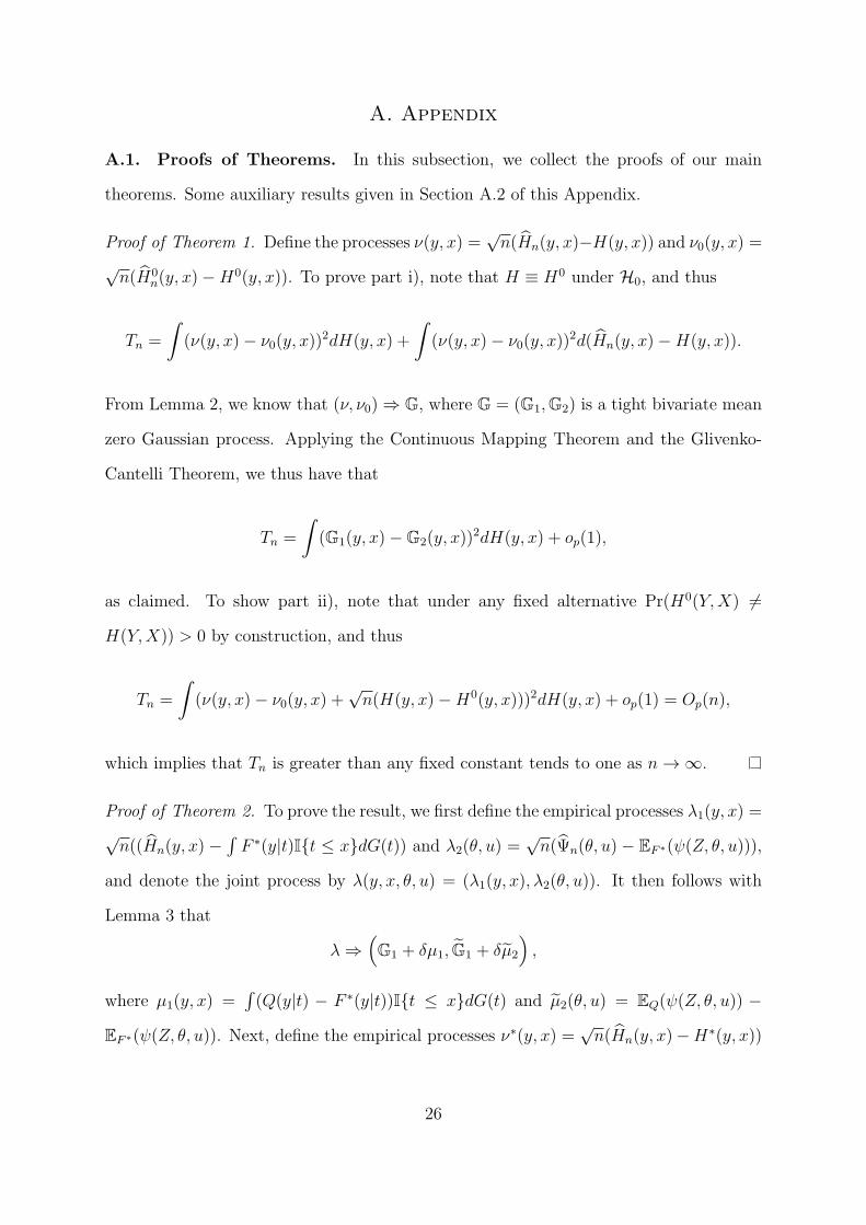
A. Appendix

A.1. Proofs of Theorems. In this subsection, we collect the proofs of our main

theorems. Some auxiliary results given in Section A.2 of this Appendix.

Proof of Theorem 1. Define the processes ν(y, x) =√n(Hn(y, x)−H(y, x)) and ν0(y, x) =

√n(H0

n(y, x)−H0(y, x)). To prove part i), note that H ≡ H0 under H0, and thus

Tn =

∫(ν(y, x)− ν0(y, x))

2dH(y, x) +

∫(ν(y, x)− ν0(y, x))

2d(Hn(y, x)−H(y, x)).

From Lemma 2, we know that (ν, ν0) ⇒ G, where G = (G1,G2) is a tight bivariate mean

zero Gaussian process. Applying the Continuous Mapping Theorem and the Glivenko-

Cantelli Theorem, we thus have that

Tn =

∫(G1(y, x)−G2(y, x))

2dH(y, x) + op(1),

as claimed. To show part ii), note that under any fixed alternative Pr(H0(Y,X) =

H(Y,X)) > 0 by construction, and thus

Tn =

∫(ν(y, x)− ν0(y, x) +

√n(H(y, x)−H0(y, x)))2dH(y, x) + op(1) = Op(n),

which implies that Tn is greater than any fixed constant tends to one as n→ ∞.

Proof of Theorem 2. To prove the result, we first define the empirical processes λ1(y, x) =

√n((Hn(y, x)−

∫F ∗(y|t)I{t ≤ x}dG(t)) and λ2(θ, u) =

√n(Ψn(θ, u)− EF ∗(ψ(Z, θ, u))),

and denote the joint process by λ(y, x, θ, u) = (λ1(y, x), λ2(θ, u)). It then follows with

Lemma 3 that

λ⇒(G1 + δµ1, G1 + δµ2

),

where µ1(y, x) =∫(Q(y|t) − F ∗(y|t))I{t ≤ x}dG(t) and µ2(θ, u) = EQ(ψ(Z, θ, u)) −

EF ∗(ψ(Z, θ, u)). Next, define the empirical processes ν∗(y, x) =√n(Hn(y, x)−H∗(y, x))

26

and ν∗0(y, x) =√n(H0

n(y, x) − H∗(y, x)), with H∗(y, x) =∫F ∗(y|t)I{t ≤ x}dG(t). Pro-

ceeding in the same way as in the proof of Lemma 2, we find that

(ν, ν0) ⇒ (G1 + δµ1,G2 + δµ2),

where µ2(y, x) =∫F (y|t)[h]I{t ≤ x}dG(t) and h(u) = ∂θ′ΨF ∗(θ∗(u), u)

−1ΨQ(θ∗(u), u).

The statement of the Theorem then follows from the continuous mapping theorem, in

the same way as in the proof of Theorem 1.

Proof of Theorem 3. To prove part i) let c(α) be the “true” critical value satisfying

P (Tn > c(α)) = α + o(1). Then it follows from Lemma 4 that cn(α) = c(α) + op(1).

This implies that Tn and Tn = Tn − (cn(α)− c(α)) converge to the same limiting distri-

bution as n→ ∞, and hence we have that P (Tn > cn(α)) = α + o(1) as claimed.

To prove part ii), note that by Lemma 4 the bootstrap critical value c(α) is bounded

in probability under fixed alternatives. Thus for any ϵ > 0 there exists a constant M

such that P (cn(α) > M) < ϵ+ o(1). Using elementary inequalities, we also have that

P (Tn ≤ cn(α)) = P (Tn ≤ cn(α), Tn ≤M) + P (Tn ≤ cn(α), Tn > M)

≤ P (Tn ≤M) + P (cn(α) > M).

From Theorem 1(ii), we know that P (Tn ≤M) = o(1), and thus P (Tn ≤ cn(α)) < ϵ+o(1),

which implies the statement of the theorem since ϵ can be chosen arbitrarily small.

To show part iii), define c(α) as in the proof of part i), i.e. the α-quantile of the

limiting distribution of the test statistic Tn under the null hypothesis. Using Anderson’s

Lemma, we find that

P

(∫(G1(y, x)−G2(y, x) + µ(y, x))2 dH(y, x) > c(α)

)≥ P

(∫(G1(y, x)−G2(y, x))

2 dH(y, x) > c(α)

)= α,

27

because the Gaussian process G1−G2 has mean zero (see also Andrews (1997, p. 1114)).

Under a local alternative, we therefore have that P (Tn > c(α)) ≥ α+ o(1). Furthermore,

we have already shown in part i) that P (Tn > cn(α)) = P (Tn > c(α)) + o(1) under the

null hypothesis. By using contiguity arguments, this can also shown to be true under the

local alternative, see e.g. the proof of Corollary 2.1 in Bickel and Ren (2001).

Proof of Theorem 4–6. This follows by straightforward applications of results in Cher-

nozhukov et al. (2009, Section 5 and Appendix D).

A.2. Auxiliary Results. In this subsection, we collect a number of auxiliary results

used in the proofs of our main results above.

Lemma 1. Define the empirical processes ν(y, x) =√n(Hn(y, x)−H(y, x)) and w(θ, u) =

√n(Ψn(θ, u)−Ψ(θ, u)). Then, under either the null hypothesis or a fixed alternative, and

Assumptions 1-6, it holds that (v, w) ⇒ G in l∞(Z × Θ × U), where G = (G1, G2) is a

tight bivariate mean zero Gaussian process. Moreover, the bootstrap procedure in Section

2.3 consistently estimates the law of G.

Proof. This lemma is a minor generalization of Lemma 13 in Chernozhukov et al. (2009),

and can thus be proven in the same way.

Lemma 2. Let either the null hypothesis or a fixed alternative, and Assumptions 1-6

be true. Define the empirical processes ν(y, x) =√n(Hn(y, x)−H(y, x)) and ν0(y, x) =

√n(H0

n(y, x) − H0(y, x)). Then it holds that (ν, ν0) ⇒ G in l∞(Z × Z), where G =

(G1,G2) is a tight bivariate mean zero Gaussian process.

Proof. Under either the null hypothesis or a fixed alternative, it follows from our Lemma

1 and Lemma 11 in Chernozhukov et al. (2009) that

√n(Hn(·, ·)−H(·, ·), θn(·)− θ0(·)) ⇒ (G1(·, ·),−Ψ−1

θ0(·),·[G2(θ0(·), ·)])

28

in ℓ∞(Z)× ℓ∞(U). Next, it follows from Assumption 5 that

√n(Fn(y|x)− F (y|x)) ⇒ −F (y|x, θ0)[Ψ−1

θ0(·),·[G2(θ0(·), ·)]] =: G∗2(y, x).

The statement of the Lemma then follows directly from Hadamard differentiability of

the mapping (A,B) 7→∫A(·, t)I{t ≤ ·}dB(t), and the Functional Delta Method. In

particular, for the second component G2 of the joint limiting process we have that

G2(y, x) =

∫F (y|t)I{t ≤ x}dG1(∞, t) +

∫G∗

2(y, t)I{t ≤ x}dG(t),

which follows from the Hadamard differential of (A,B) 7→∫A(·)I{t ≤ ·}dB(t).

Lemma 3. Suppose the data are distributed according to a local alternative Qn sat-

isfying Assumption 7. Define the processes vn(y, x) =√n(Hn(y, x) − Hn(y, x)) and

wn(θ, u) =√n(Ψn(θ, u) − Ψn(θ, u)), where Hn(y, x) =

∫Qn(y|t)I{t ≤ x}dG(t) and

Ψn(θ, u) = EQn(ψ(Z, θ, u)). Then it holds (vn, wn) ⇒ G in l∞(Z × Θ × U), where the

limiting process G has the same properties as the one in Lemma 1.

Proof. This follows by an application of Lemma 2.8.7 in Van der Vaart and Wellner

(1996), using the fact that by Assumption 4, Qn is the linear combination of two measures

under which the function class G is Donsker with a square integrable envelope.

Lemma 4. Define the bootstrap empirical processes νb(y, x) =√n(Hb,n(y, x)− H0

n(y, x))

and νb,0(y, x) =√n(H0

b,n(y, x)− H0n(y, x)). Then it holds under either the null hypothesis

or a fixed alternative that (νb, νb,0) ⇒ Gb, where Gb = (Gb1,Gb2) is a tight bivariate mean

zero Gaussian process whose distribution coincides with that of the process G in Lemma 1

under the null hypothesis.

Proof. This follows from Lemma 1 and the Functional Delta Method for the bootstrap

(Van der Vaart and Wellner, 1996, Theorem 3.9.11)

29

References

Andrews, D. (1997): “A conditional Kolmogorov test,” Econometrica, 65, 1097–1128.

Beran, R. (1988): “Prepivoting test statistics: a bootstrap view of asymptotic refine-

ments,” Journal of the American Statistical Association, 687–697.

Bickel, P. and J.-J. Ren (2001): “The bootstrap in hypothesis testings,” Lecture

Notes-Monograph Series, 36, 91–112.

Bierens, H. (1990): “A consistent conditional moment test of functional form,” Econo-

metrica, 1443–1458.

Bierens, H. and D. Ginther (2001): “Integrated conditional moment testing of quan-

tile regression models,” Empirical Economics, 26, 307–324.

Bierens, H. and W. Ploberger (1997): “Asymptotic theory of integrated conditional

moment tests,” Econometrica, 65, 1129–1151.

Billingsley, P. (1995): Probability and measure, Wiley.

Chernozhukov, V., I. Fernandez-Val, and B. Melly (2009): “Inference on Coun-

terfactual Distributions,” Working Paper.

DiNardo, J., N. Fortin, and T. Lemieux (1996): “Labor market institutions and

the distribution of wages, 1973-1992: A semiparametric approach,” Econometrica, 64,

1001–1044.

Escanciano, J. and C. Goh (2010): “Specification Analysis of Structural Quantile

Regression Models,” Working Papers.

Escanciano, J. and C. Velasco (2010): “Specification tests of parametric dynamic

conditional quantiles,” Journal of Econometrics, 159, 209–221.

Foresi, S. and F. Peracchi (1995): “The Conditional Distribution of Excess Returns:

An Empirical Analysis.” Journal of the American Statistical Association, 90, 451–466.

30

Fortin, N., T. Lemieux, and S. Firpo (2011): “Decomposition Methods in Eco-

nomics,” Handbook of Labor Economics, 4, 1–102.

Galvao, A., K. Kato, G. Montes-Rojas, and J. Olmo (2011): “Testing linearity

against threshold effects: uniform inference in quantile regression,” Working Paper.

Hall, P. (1986): “On the bootstrap and confidence intervals,” The Annals of Statistics,

1431–1452.

Hardle, W. and E. Mammen (1993): “Comparing nonparametric versus parametric

regression fits,” The Annals of Statistics, 21, 1926–1947.

Harvey, A. (1976): “Estimating regression models with multiplicative heteroscedastic-

ity,” Econometrica, 461–465.

He, X. and L. Zhu (2003): “A lack-of-fit test for quantile regression,” Journal of the

American Statistical Association, 98, 1013–1022.

Horowitz, J. and V. Spokoiny (2001): “An Adaptive, Rate-Optimal Test of a Para-

metric Mean-Regression Model Against a Nonparametric Alternative,” Econometrica,

69, 599–631.

——— (2002): “An adaptive, rate-optimal test of linearity for median regression models,”

Journal of the American Statistical Association, 97, 822–835.

Koenker, R. (2005): Quantile regression, Cambridge University Press.

——— (2010): “On Distributional vs. Quantile Regression,” Working Paper.

Koenker, R. and G. Bassett (1978): “Regression quantiles,” Econometrica, 46, 33–

50.

Koenker, R. and J. Machado (1999): “Goodness of fit and related inference processes

for quantile regression,” Journal of the American Statistical Association, 94, 1296–1310.

31

Koenker, R. and Z. Xiao (2002): “Inference on the quantile regression process,”

Econometrica, 70, 1583–1612.

Machado, J. and J. Mata (2005): “Counterfactual decomposition of changes in wage

distributions using quantile regression,” Journal of Applied Econometrics, 20, 445–465.

Powell, J. (1986): “Censored regression quantiles,” Journal of Econometrics, 32, 143–

155.

Rothe, C. (2010): “Nonparametric Estimation of Distributional Policy Effects,” Journal

of Econometrics, 155, 56–70.

——— (2011): “Partial Distributional Policy Effects,” Econometrica (to appear).

Rothe, C. and D. Wied (2012): “Misspecification Testing in a Class of Conditional

Distributional Models,” IZA Working Paper.

Rutemiller, H. and D. Bowers (1968): “Estimation in a heteroscedastic regression

model,” Journal of the American Statistical Association, 552–557.

Stute, W. (1997): “Nonparametric model checks for regression,” The Annals of Statis-

tics, 613–641.

Van der Vaart, A. and J. Wellner (1996): Weak convergence and empirical pro-

cesses: with applications to statistics, Springer Verlag.

Whang, Y.-J. (2006): “Consistent Specification Testing for Quantile Regression Mod-

els,” in Econometric Theory and Practice: Frontiers of Analysis and Applied Research,

ed. by D. Corbae, S. Durlauf, and B. Hansen, Cambridge University Press.

Zheng, J. (1998): “A consistent nonparametric test of parametric regression models

under conditional quantile restrictions,” Econometric Theory, 14, 123–138.

32